Deep learning joint extremes of metocean variables using the SPAR model

Abstract

This paper presents a novel deep learning framework for estimating multivariate joint extremes of metocean variables, based on the Semi-Parametric Angular-Radial (SPAR) model. When considered in polar coordinates, the problem of modelling multivariate extremes is transformed to one of modelling an angular density, and the tail of a univariate radial variable conditioned on angle. In the SPAR approach, the tail of the radial variable is modelled using a generalised Pareto (GP) distribution, providing a natural extension of univariate extreme value theory to the multivariate setting. In this work, we show how the method can be applied in higher dimensions, using a case study for five metocean variables: wind speed, wind direction, wave height, wave period and wave direction. The angular variable is modelled empirically, while the parameters of the GP model are approximated using fully-connected deep neural networks. Our data-driven approach provides great flexibility in the dependence structures that can be represented, together with computationally efficient routines for training the model. Furthermore, the application of the method requires fewer assumptions about the underlying distribution(s) compared to existing approaches, and an asymptotically justified means for extrapolating outside the range of observations. Using various diagnostic plots, we show that the fitted models provide a good description of the joint extremes of the metocean variables considered.

1 Introduction

Many problems in offshore and coastal engineering require estimation of joint extremes for metocean variables. Responses of offshore and coastal structures are dependent on multiple variables, such as wind speed and direction, wave height, period and direction, current speed and direction. Providing accurate and reliable estimates of the joint extremes in this setting is a challenging problem for metocean engineers. Various design standards recommend the use of the environmental contour method [1]. Some types of contour can be estimated without an explicit model for the joint distribution of variables [2, 3]. However, environmental contour methods typically make simplifying assumptions and only give approximate estimates of long-term extreme responses [4, 5]. Full probabilistic analysis of long-term extreme responses requires a model for the joint density of the relevant metocean variables. A wide range of approaches have been proposed for estimating joint densities. In the offshore engineering literature, the two most popular approaches are global hierarchical models and copula models – see, e.g. [6, 7].

Let $\mathbf{X}=(X_{1},...,X_{d})\in\mathbb{R}^{d}$ denote a continuous random vector with joint density function $f_{\mathbf{X}}$, and marginal density and distribution functions $f_{X_{j}}$ and $F_{X_{j}},$ respectively, for $j=1,...,d$. In the global hierarchical approach [8, 9, 10], the joint density is written as

$$f_{\mathbf{X}}(\mathbf{x})=f_{X_{1}}(x_{1})\,f_{X_{2}|X_{1}}(x_{2}|x_{1})\cdots f_{X_{d}|(X_{1},...,X_{d-1})}(x_{d}|(x_{1},...,x_{d-1})),$$ (1)

where $f_{X_{j}|(X_{1},...,X_{j-1})}$ is the density of $X_{j}$ conditional on $(X_{1},...,X_{j-1})$ for $j\in\{2,\ldots,d\}$. Inference typically involves selecting parametric forms for $f_{X_{1}}(x_{1})$, $f_{X_{2}|X_{1}}$, …, $f_{X_{d}|(X_{1},...,X_{d-1})}$ and estimating relations between the parameters of the conditional densities and the conditioning variables. There are various problems with this approach. Firstly, there is no a priori reason to suppose that variables follow any particular parametric distribution, and misspecified models can have dramatic consequences when approximating dependence structures. Secondly, a model fit to all of the observations does not guarantee a good fit to the tail, which is the region of interest for extremes. Finally, the models for the parameters of the conditional densities are usually based on ad hoc assumptions, and provide no rationale for extrapolating outside the range of observations. In many cases, it has been shown that such models provide a poor fit to observed data [11].

For copula modelling, the joint density is written as

$$f_{\mathbf{X}}(\mathbf{x})=f_{X_{1}}(x_{1})\cdots f_{X_{d}}(x_{d})c(F_{X_{1}}(x_{1}),\cdots,F_{X_{d}}(x_{d})),$$ (2)

where $c:[0,1]^{d}\mapsto[0,\infty)$ is the copula density of $\mathbf{X}$ [12]. In this case, inference involves choosing parametric models for both the marginal densities and for $c$. As with the global hierarchical approach, there are no a priori reasons to choose particular models. Similarly, fitting to all observations does not guarantee a good fit to the tails. Moreover, different copula models have very different behaviours in the joint tail regions, meaning extrapolation can vary substantially for different choices of copula model [12].

There are also a wide range of methods in the statistical literature for modelling joint extremes (e.g. [13, 14, 15]). However, many of these approaches make strong assumptions about the dependence structure, or copula, which are often not supported by environmental datasets [16]. The most popular choice for metocean variables is the conditional extremes model [17], which describes the joint distribution of variables conditional on at least one variable being large. The key limitation of this approach is that it only characterises the region of variable space where the conditioning variable is large, and inferences made using different conditioning variables are not necessarily consistent [18]. A further limitation of this method (and other methods in the multivariate extremes literature) is that it requires a transformation of the margins to a standard scale. This requires first estimating the marginal distributions for each variable – a process which is subject to uncertainty. Furthermore, it has been demonstrated that poor marginal estimates greatly affect the quality of the resulting multivariate inference [19].

In this paper, we discuss the application of a new method, introduced in [20], which overcomes the limitations of existing approaches and provides a general, flexible framework for modelling multivariate extremes. The model is referred to as the Semi-Parametric Angular-Radial (SPAR) model. The SPAR model provides a framework for estimating multivariate extremes that does not require strong assumptions about the form of the margins or dependence structure, and provides a justified means of extrapolating outside the range of observations. Moreover, the model is only fitted to extreme observations, meaning that no assumptions are required about the bulk of the distribution. Theoretical aspects of the SPAR model are presented in [21], and an inference approach in a two-dimensional setting is provided in [22, 23]. The purpose of this paper is to extend the modelling method to the general multivariate setting.

The paper is organised as follows. Section 2 describes a brief overview of the theoretical aspects of the model. Our deep learning approach for estimating SPAR model parameters is introduced in Section 3. Section 4 presents an example application of the model to a five-dimensional problem: estimating the joint extremes of wind speed, wave direction, wave height, wave period and wave direction. We discuss the challenges that arise for these particular variables, and how well the model assumptions are satisfied in this setting. We conclude in Section 5 with a discussion and outlook on future work.

2 Theory

The SPAR model is an extension of the univariate peaks-over-threshold (POT) method to the multivariate setting. It involves a transformation of variables to angular-radial coordinates, and then models the upper-tail of the radial variable, conditional on angle, using a non-stationary generalised Pareto (GP) model. Suppose that we have a continuous random vector $\mathbf{X}=(X_{1},...,X_{d})\in\mathbb{R}^{d}$ with joint density function $f_{\mathbf{X}}$. We define radial and angular variables as

$$R=\|\mathbf{X}\|_{2},\quad\mathbf{W}=\mathbf{X}/R,$$ (3)

where $\|\cdot\|_{2}$ is the $L^{2}$ or Euclidean norm, defined by $\|(x_{1},...,x_{d})\|_{2}=(x_{1}^{2}+\cdots+x_{d}^{2})^{1/2}$. Note that $R\in[0,\infty)$ and $\mathbf{W}\in\mathbb{S}^{d-1}$, where $\mathbb{S}^{d-1}=\{\mathbf{x}\in\mathbb{R}^{d}:\|\mathbf{x}\|_{2}=1\}$ is the unit hypersphere in $\mathbb{R}^{d}$. The joint density function of $(R,\mathbf{W})$ is related to $f_{\mathbf{X}}$ via

$$f_{R,\mathbf{W}}(r,\mathbf{w})=r^{d-1}\,f_{\mathbf{X}}(r\mathbf{w}),$$ (4)

where $r^{d-1}$ is the Jacobian determinant for the transformation $\mathbf{X}\rightarrow(R,\mathbf{W})$. As for global hierarchical models, the angular-radial joint density can be written in conditional form as:

$$f_{R,\mathbf{W}}(r,\mathbf{w})=f_{\mathbf{W}}(\mathbf{w})\,f_{R|\mathbf{W}}(r|\mathbf{w}).$$ (5)

Noting that $\mathbf{X}=R\mathbf{W}$, and that $\mathbf{W}$ lies on the surface of the unit hypersphere, we can see that the ‘extreme’ parts of the distribution of $\mathbf{X}$ correspond to large values of the radial variable at any given angle. Therefore, the problem of modelling multivariate extremes is transformed to that of modelling an angular density $f_{\mathbf{W}}$ and the tail of the conditional radial density $f_{R|\mathbf{W}}$. For a given angle $\mathbf{w}$, the density $f_{R|\mathbf{W}}(r|\mathbf{w})$ is univariate. Univariate extreme value theory suggests that a suitable model for the tail of $f_{R|\mathbf{W}}$ is the GP distribution, with parameters conditional on angle (e.g., [24]). This motivates the SPAR model, whereby parametric and non-parametric models are used to model the conditional radial and angular distributions, respectively. Define a threshold function $u(\mathbf{w})>0$ to be the quantile of $R|(\mathbf{W}=\mathbf{w})$ at exceedance probability $\zeta\in(0,1)$, with $\zeta$ close to 0, i.e., the solution of $\zeta=\Pr(R>u(\mathbf{w})|\mathbf{W}=\mathbf{w})$. The SPAR model can be written as

$$f_{R,\mathbf{W}}(r,\mathbf{w})=\zeta f_{\mathbf{W}}(\mathbf{w})f_{GP}(r-u(\mathbf{w});\xi(\mathbf{w}),\sigma(\mathbf{w})),\quad r>u(\mathbf{w}),$$ (6)

where $f_{GP}$ is the GP density function, and $\xi(\mathbf{w})\in\mathbb{R}$ and $\sigma(\mathbf{w})>0$ are shape and scale parameters, respectively, given as functions of the angle $\mathbf{w}$. The GP density function is given by

$$f_{GP}(r;\xi,\sigma)=\begin{cases}\dfrac{1}{\sigma}\left(1+\xi\dfrac{r}{\sigma}\right)^{-1-\tfrac{1}{\xi}},&\xi\neq 0,\\[10.0pt] \dfrac{1}{\sigma}\exp\left(-\dfrac{r}{\sigma}\right),&\xi=0,\end{cases}$$ (7)

which is supported on $0\leq r\leq r^{F}$, where $r^{F}=\infty$ for $\xi\geq 0$ and $r^{F}=-\sigma/\xi$ for $\xi<0$.

Many non-parametric methods for estimation of densities assume that the density is finite and continuous. Similarly, many representations for non-stationary modelling of parametric distributions assume that the parameter functions are finite and continuous. Therefore, to simplify our inference, we assume that the angular density $f_{\mathbf{W}}$, threshold function $u(\mathbf{w})$, and GP parameter functions, $\xi(\mathbf{w})$ and $\sigma(\mathbf{w})$ are finite and continuous with respect to the angle $\mathbf{w}$.

After estimation of the angular density and GP parameter functions, (4) and (6) can be combined to obtain the SPAR estimate of the joint density in the original variable space for observations satisfying $r>u(\mathbf{w})$, i.e.,

$$f_{\mathbf{X}}(r\mathbf{w})=\zeta\,r^{1-d}\,f_{\mathbf{W}}(\mathbf{w})\,f_{GP}(r-u(\mathbf{w});\xi(\mathbf{w}),\sigma(\mathbf{w})).$$ (8)

Calculating marginal and joint probabilities using the SPAR model then involves either integration of the joint density over specified angular and radial domains, or via Monte Carlo techniques, i.e., by simulating from the estimated model and deriving probability estimates empirically. To simulate from the SPAR model, we first draw an angle $\mathbf{w}$ from $f_{\mathbf{W}}$, then use inversion sampling to generate a corresponding radial value $z$ from the GP distribution with parameter vector $(\xi(\mathbf{w}),\sigma(\mathbf{w}))$, and finally define $r=u(\mathbf{w})+z$. The pair $(r,\mathbf{w})$ is then a random sample from the SPAR model. This can be converted back to the original variable space using the inverse transformation $\mathbf{x}=r\mathbf{w}$. As the SPAR model is only fitted to observations for which $r>u(\mathbf{w})$, one can create a sample (of the original random vector $\mathbf{X}$) of size $N$ by simulating $\zeta N$ points from the SPAR model, and then resampling $(1-\zeta)N$ points from observations with $r<u(\mathbf{w})$. The rationale for this is that there should be a sufficient number of observations within the body of the distribution to obtain a reasonable estimate from resampling.

As described in [23], the SPAR model provides an explicit means for calculating a contour with a specified exceedance probability. However, this contour is defined in terms of the probability of an observation falling anywhere outside the region, or the ‘total exceedance probability’. As such, these contours are more conservative than those defined in terms of marginal exceedance probabilities, such as IFORM contours (or variants thereof), with the conservatism increasing with the number of dimensions [25]. If the primary interest of the analysis is to estimate environmental contours, then the use of the SPAR model is not necessary. Instead, we recommend the use of the Direct-IFORM method [2, 3], which does not require a model for the joint density or any assumptions about the dependence structure between the variables.

3 Inference

Inference for the SPAR model involves estimating the angular density, and the GP threshold and parameter functions. These problems are separable: inference for $f_{\mathbf{W}}$ can be conducted independently of that for $(u(\mathbf{w}),\sigma(\mathbf{w}),\xi(\mathbf{w}))$. In this section, we discuss inference for the angular density in Section 3.1, then discuss modelling of the conditional radial variable in Section 3.2. Code for fitting our model is available upon reasonable request.

3.1 Angular modelling

Estimation of densities on the hypersphere $\mathbb{S}^{d-1}$ is part of a discipline known as directional statistics [26, 27, 28]. The key difference from estimation of densities on $\mathbb{R}^{d}$ is that the surface of the hypersphere is periodic and bounded, and so distributions defined on $\mathbb{S}^{d-1}$ must conserve these constraints. Various parametric and non-parametric approaches have been developed for estimating densities on the hypersphere, which are directly analogous to approaches used in Euclidean space. These include kernel density estimation [29, 30], mixture models [31, 32], and spline-based methods [33]. See [28] for a recent review of non-parametric approaches.

Previous uses of SPAR in two dimensions adopted a kernel density method for estimating the angular density. Although this approach can be applied in higher dimensions, simulation from the estimated density can be very slow, as it requires transformation to hyperspherical coordinates and numerical integration to obtain conditional distributions. The use of parametric mixture models instead results in faster simulation. However, for the application described in Section 4, we found that a mixture of $d$-variate von Mises distributions [34] was not flexible enough to capture the complex structure in the angular data, even with hundreds of mixture components. Moreover, spline-based approaches have only been proposed for $d\leq 3$, and are therefore not applicable for the setting we consider.

As noted in Section 2, an estimate of the angular density function $f_{\mathbf{W}}$ is required to approximate the joint density of the random vector $\mathbf{X}$. However, to simulate from the SPAR model, one only requires a means of simulating from the angular variable $\mathbf{W}$; an explicit form for the density is not a necessity. Consequently, for our approach, we opt to sample the angular component empirically, i.e., we draw from the observed sample $\{\mathbf{w}_{1},\ldots,\mathbf{w}_{n}\}$ with replacement. Since the angular variable lies in a bounded domain (the surface of the hypersphere), values of $\mathbf{W}$ are never ‘extreme’. Therefore, given a sufficiently large sample size $n$, empirical resampling should provide a representative sample of the angular variable $\mathbf{W}$ for all regions of $\mathbb{S}^{d-1}$ where this variable has probability mass. Providing that we can also simulate from the conditional radial variable, $R|\mathbf{W}=\mathbf{w},$ we can generate new, representative data in the joint tail of $\mathbf{X}$. However, as discussed further in Section 4, in regions where angular observations are sparse, resampling does not give us a method of simulating unobserved, but plausible angles. Alternative methods of modelling angular density will be examined in future work.

3.2 Conditional radial modelling

Viewing the angular variable $\mathbf{W}$ as a ‘covariate’ for the radial variable $R$, inference for the SPAR model is analogous to a non-stationary POT analysis, for which many parametric and semi-parametric approaches have been proposed [35, 36, 37, 38, 39]. Non-stationary POT can be performed using GP regression (modelling GP parameters as functions of covariates), which proceeds by first estimating the threshold function, $u(\mathbf{w})$, and then estimating the GP scale and shape parameter functions, $\sigma(\mathbf{w})$ and $\xi(\mathbf{w})$ respectively, via likelihood-based inference procedures. The choice of the functional forms for $u(\mathbf{w})$, $\sigma(\mathbf{w})$, and $\xi(\mathbf{w})$ determine the flexibility of the overall model. As the dimension $d$ grows, these mappings become increasingly complex, and so models that represent the functions via semi-parametric models (such as the splines used in initial work with the SPAR model [22] and other similar angular-radial approaches [40, 41]) are unlikely to offer sufficient flexibility. Moreover, they become increasingly computationally-demanding to estimate for large $d$. Consequently, we adopt a deep learning approach, whereby the threshold and GP parameter functions are represented using artificial neural networks (ANN); for details on GP regression with deep learning, see [42]. Although the representation of the SPAR parameter functions via ANNs differs from previous approaches in this framework, the ‘loss function’ used for optimisation of the model, is the same. That is, we estimate the threshold and GP parameter functions that maximise the likelihood evaluated on a hold-out dataset, as described in Section 3.2.2. This work builds upon the approach of [43], who use deep learning to estimate the extremal dependence structure of random vectors on standardised marginal scales via a similar angular-radial decomposition. In contrast, our approach does not require marginal transformation, and is thus not subject to marginal estimation uncertainty.

3.2.1 Neural network representation of conditional radial parameters

Several recent approaches have used deep learning for GP regression; see, e.g. [44, 45, 46, 47]. In these approaches, ANNs are used to model the relationships between covariates and GP parameter and threshold functions. Our approach is analogous, with the covariates taken to be angles on the hypersphere. Note that the hypersphere is compact (i.e., closed and bounded), and that this is a desirable property for extrapolation in deep learning.

Here, we design two neural network models; one for the threshold function $u(\mathbf{w})$ and one for the parameter vector $(\nu(\mathbf{w}),\xi(\mathbf{w}))$, where $\nu(\mathbf{w})=\sigma(\mathbf{w})(\xi(\mathbf{w})+1)$ is the modified scale parameter. Unlike $\sigma(\mathbf{w})$, the modified scale parameter $\nu(\mathbf{w})$ is orthogonal to $\xi(\mathbf{w})$, which helps to mitigate numerical instabilities during model fitting [48, 35, 49]; [47] show that this is particularly helpful when estimating deep GP regression models. Both $u(\mathbf{w})$ and $(\nu(\mathbf{w}),\xi(\mathbf{w}))$ are modelled by multi-layer perceptrons (MLPs), which are a standard class of fully-connected ANN that compose multiple layers of ‘neurons’ [50]. Each neuron passes a linear combination of input variables through a nonlinear ‘activation function’, and the output is then passed to the subsequent layer; detailed discussions and illustrative figures can be found in [42], and an example schematic for an MLP representation of $(\nu(\mathbf{w}),\xi(\mathbf{w}))$ is presented in Figure 1. Inference for the parameter functions then involves estimating the linear coefficients (the ‘weights’ and ‘biases’) in each neuron of the corresponding MLP. Prior to inference, the architecture of the MLP must be defined, i.e., the number of hidden layers, denoted by $L$, the number of neurons in each hidden layer, denoted by $h_{1},\ldots,h_{L}$, and the type(s) of activation function(s). The resulting set of estimable parameters for the MLP contains all of the weights and biases in each hidden layer, as well as the final $(L+1)$-th layer; we denote this by $\mathcal{W}=\left\{\left(a^{l},b^{l}\right);l=1,\ldots,L+1\right\}$, with weights $a^{l}\in\mathbb{R}^{h_{l}\times h_{l-1}}$ and biases $b^{l}\in\mathbb{R}^{h_{l}}$. Note that the estimable sets of parameters differ between the MLPs for $u(\mathbf{w})$ and $(\nu(\mathbf{w}),\xi(\mathbf{w}))$; we denote their respective parameter sets by $\mathcal{W}_{u}$ and $\mathcal{W}_{(\nu,\xi)}$. For both MLPs, we take all hidden layer activation functions to be the rectified linear unit function, $\text{ReLU}(\mathbf{x})=(\max\{x_{1},0\},\max\{x_{2},0\},\dots)$. The final layers of the MLPs make use of an exponential transformation to ensure that the scale $\nu(\mathbf{w})$ and threshold $u(\mathbf{w})$ are strictly positive, that is, $\nu(\mathbf{w})>0,u(\mathbf{w})>0$ for all $\mathbf{w}$. For numerical stability, we also ensure that $\xi(\mathbf{w})$ satisfies $\xi(\mathbf{w})\in(-0.5,0.1)$ for all angles $\mathbf{w}$. Selection of the remaining tuning parameters is discussed in Section 3.2.3.

Figure 1: Example schematic of an MLP model with $L=2$ hidden layers. The inputs are the components of the angle $\mathbf{w}=(w_{1},w_{2},...,w_{d})$ and the outputs are the GP parameter functions $(\nu(\mathbf{w}),\xi(\mathbf{w}))$.

3.2.2 Estimating the neural network parameters

To obtain estimates of the MLP parameter sets, $\mathcal{W}_{u}$ and $\mathcal{W}_{(\nu,\xi)}$, we optimise specified loss functions. Suppose that we have a set of radial and angular observations $\{(r_{i},\mathbf{w}_{i});i=1,...,n\}$. Recall from Equation (6) that the threshold $u(\mathbf{w})$ is taken to be the $1-\zeta$ quantile of $R|\mathbf{W}=\mathbf{w}$. We thus can estimate $u(\mathbf{w})$ (and its corresponding parameter set $\mathcal{W}_{u}$) using techniques from quantile regression [51]. In this case, the most appropriate loss function for $u(\mathbf{w})$ is the tilted loss,

$$\mathcal{L}_{u}(\mathcal{W}_{u}):=\sum_{i=1}^{n}\rho_{1-\zeta}\left\{r_{i}-u\left(\mathbf{w}_{i}\right)\right\},$$ (9)

where $\rho_{\alpha}(t):=t(\alpha-\mathbbm{1}\{t<0\})$ for indicator function $\mathbbm{1}$ and where dependency of $u(\mathbf{w})$ on $\mathcal{W}_{u}$ has been suppressed from notation.

After estimation of $u(\mathbf{w})$, we define $I_{u}:=\{i:r_{i}>u(\mathbf{w}_{i})\}$ as the set of indices of radial threshold exceedances. The MLP that defines the GP parameter functions can be considered as a ‘conditional density estimation network’, with the negative log-likelihood function used for optimisation; see, e.g. [52, 53]. In this case, we perform maximum likelihood estimation, and thus the loss function is given by

$$\mathcal{L}_{GP}(\mathcal{W}_{(\nu,\xi)}):=-\sum_{i\in I_{u}}\log\left[f_{GP}\left(r_{i}-u(\mathbf{w}_{i});\xi(\mathbf{w}_{i}),\frac{\nu(\mathbf{w}_{i})}{\xi(\mathbf{w}_{i})+1}\right)\right].$$ (10)

Optimisation of both losses, (9) and (10), proceeds via stochastic gradient descent and the ADAM algorithm [54]. To mitigate overfitting, data are split into training (80%) and validation (20%) sets, with the latter used to check for parameter convergence. We refer the reader to [43] for a more detailed overview of the fitting procedure.

As noted in Section 2, when the GP shape parameter $\xi(\mathbf{w})$ is negative, the distribution of $R|\mathbf{w}=\mathbf{w}$ has a finite upper endpoint. Training of a deep GP regression model which permits negative shape parameter values can be computationally troublesome; see discussion by [55]. At a given angle $\mathbf{w}_{i}$, if $\xi(\mathbf{w}_{i})<0$ and the radial observation $r_{i}$ exceeds the upper endpoint, i.e., $r_{i}>u(\mathbf{w}_{i})-\sigma(\mathbf{w}_{i})/\xi(\mathbf{w}_{i})$, then the loss function in (10) will evaluate to a non-finite value. Consequently, the loss surface over which we optimise $\mathcal{W}_{(\nu,\xi)}$ is highly irregular, and iterative gradient descent methods (like ADAM) may have trouble finding global maxima, or may predict out-of-sample parameter estimates that are infeasible, i.e., the loss is non-finite. To circumvent these issues during training, we initialise the MLP to ensure that the shape parameter function $\xi(\mathbf{w})$ is non-negative for all angles $\mathbf{w}$; in this way, at the outset of the training procedure, the loss function is guaranteed to be finite for all $w_{i},i=1,\dots,n$. Then, if the gradient descent optimisation algorithm produces non-finite loss values during training, we restart training (from the last iteration with finite loss values) with a smaller learning rate. Note that the fully-trained MLP may still provide negative values of $\xi(\mathbf{w})$. This training procedure was found to produce reliable estimates in our application.

3.2.3 Selecting an architecture

An important choice when fitting a neural network model is the choice of architecture: this corresponds to the set of hyperparameters introduced in Section 3.2.1. There is no ‘best practice’ for this selection within the deep GP regression literature [42], and the appropriate architecture is likely to be domain specific; see [50]. Selecting a model with more hidden layers and more neurons results in higher flexibility, but at the cost of increased parameter variability and computational expense. In the spirit of parsimony, we wish to select the simplest model possible while still capturing the observed variability in the threshold and GP parameter functions over the angular domain.

To select our ‘optimal’ architecture for the application detailed in Section 4, we perform a grid-search over architecture choices. For each configuration, we estimate a range of model fit diagnostics; these are discussed below. The optimal architecture is then chosen as the configuration which visually provides the best model diagnostics. We found that for both MLPs, a simple architecture is preferable: $L=3$ hidden layers, with $h_{l}=16$ neurons per layer. This results in two MLPs, each comprising approximately 650 estimable parameters; inference for these models is not computationally demanding, and can be conducted on a standard laptop.

As with univariate POT models, selecting a suitable threshold for our model is critical. Too low a threshold will result in the asymptotic arguments motivating the use of the GP model not being applicable, causing bias; whereas too high a threshold will result in few observations to fit to, resulting in higher variance. The process of threshold selection for our model is directly analogous to that in univariate problems. That is, we fit the model for a range of threshold exceedance probabilities $\zeta$, and check for stability of inferences and goodness of fit. The threshold is then selected as the largest value of $\zeta$ for which inferences are approximately stable for $\zeta_{0}<\zeta$. In our application, we found that $\zeta=0.1$ was suitable.

We remark that while our selected architecture works well for our application, we do not advocate the general use of these hyperparameters. Instead, we recommend that practitioners who apply our framework perform a similar grid-search, and and use post-fit diagnostics to select the optimal architecture.

4 Application to five-dimensional problem

4.1 Dataset

In this section, we consider the application of the SPAR model to a hindcast dataset consisting of 31-years of wind and wave variables from 01/01/1990 to 31/12/2020, for a site in the Celtic Sea, off the south-west coast of the UK, which has been identified for development of floating wind farm projects. The dataset consists of hourly values of significant wave height $(H_{s})$, mean wave period $(T_{m})$, mean wave direction $(\theta_{wave})$, hourly mean wind speed at 10 m above sea level $(U_{10})$, and wind direction $(\theta_{wind})$. These variables all influence the motion and loading of floating wind turbines, and understanding their joint extremes is important for design. Since directional variables are periodic, it does not make sense to talk about ‘extreme directions’. Instead, we work with the x- and y-components of wave height and wind speed, defined as $H_{x}=H_{s}\cos(\theta_{wave})$, $H_{y}=H_{s}\sin(\theta_{wave})$, $U_{x}=U_{10}\cos(\theta_{wind})$, and $U_{y}=U_{10}\sin(\theta_{wind})$.

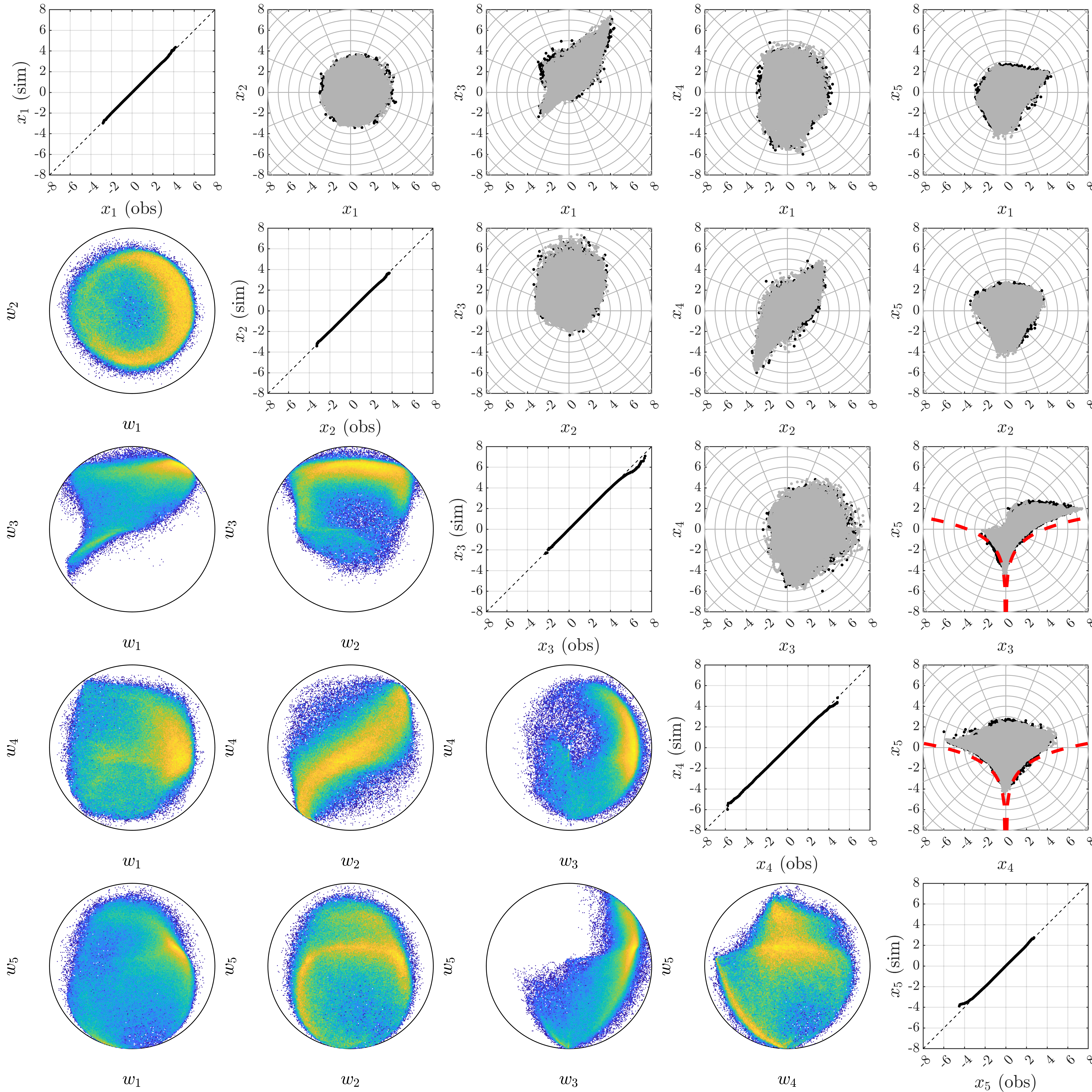
Figure 2: Upper right plots: Scatter of pairwise relations between normalised variables for simulated (black) and observed (grey) data. Dashed red lines in plots of $(x_{3},x_{5})$ and $(x_{4},x_{5})$ are lines of constant wave steepness $s=0.08$. Plots on diagonal are QQ plots of simulated vs observed data. Lower left plots: Empirical density of pairs of angular components of observed data (yellow = high density, blue = low density).

Unlike many classical modelling approaches, the SPAR approach extrapolates in all directions, allowing one to perform inference in any extreme region of interest. When variables have a defined lower bound at zero, as is the case for many physical quantities, the SPAR model should be able to infer this directly from the data, and these physical limits should correspond to the upper bounds of the GP model for the radial variable at the relevant angles. However, inferences at end points are highly uncertain since they correspond to zero exceedance probability, and consequently the model may infer a slightly negative bound in some directions. It is therefore safer to work with variables that do not have hard lower bounds at zero, so that uncertainties in the radial end point do not result in estimates that are not physically possible. The directional variables $H_{x}$, $H_{y}$, $U_{x}$, and $U_{y}$ are all defined on $(-\infty,\infty)$, although clearly they will have some upper and lower bounds due to physical constraints (in general, we would expect the region of variable space in which the density is non-zero to be bounded, due to physical limits). For the period variable, we address the problem of the lower bound by defining $L_{T}=\log(T_{m})\in(-\infty,\infty)$ and using this variable in the model.

4.2 Normalisation and choice of origin

As different physical variables have different scales, we normalise each variable by its standard deviation. If we did not do this, then angles would tend to be clustered in the plane of whichever variable has the largest scale (wind speed in this case). We also need to define an origin in order to transform to polar coordinates. In previous work using SPAR, [23, 22] defined the origin at the mean of each variable. In our application, more care must be taken when defining an appropriate origin. For the model to provide a useful description of the extremes at all angles, the support of the density, $\mathrm{supp}(f_{\mathbf{X}}):=\{\mathbf{x}\in\mathbb{R}^{d}:f_{\mathbf{X}}(\mathbf{x})>0\}$, must be star-shaped with respect to the chosen origin [56]. That is, given an origin $\mathbf{x}_{0}\in\mathbb{R}^{d}$ and any point $\mathbf{x}\in\mathrm{supp}(f_{\mathbf{X}})$, the line segment from $\mathbf{x}_{0}$ to $\mathbf{x}$ is contained in $\mathrm{supp}(f_{\mathbf{X}})$. Under this assumption, all rays from the origin reach the ‘edges’ of the distribution without passing through regions which have zero density. In this way, the data-cloud has a well-defined ‘inside’ and ’outside’, with the ‘outer’ region considered ‘extreme’, and the representation of the radial component in this region by a GP distribution is reasonable. This assumption can be verified by checking plots of the density of observations along various rays from the origin, e.g., histograms of the observed radial variable within small angular ranges. However, as discussed further below, in higher dimensional spaces, a large number of angles are required to obtain a reasonable coverage of the surface of $\mathbb{S}^{d-1}$, and visual inspection of plots of the radial density over each angular range is time consuming. Ultimately a data-driven approach for selecting an optimal choice of origin would be best.

In this example, we use some physical insights to define an appropriate origin. Firstly, wave breaking limits the maximum possible wave height for a given wave period, with the limit related to wave steepness given by $s=2\pi H_{s}/(gT_{m}^{2})$. In the three-dimensional subspace containing the variables $(H_{x},H_{y},T_{m})$, this results in a conical-shaped bound on the data, centred along the axis $H_{x}=H_{y}=0$, with the radius of the cone given by $H_{s,max}=s_{max}gT_{m}^{2}/(2\pi)$, where $s_{max}$ is the limiting steepness. The limit value of $s_{max}$ depends on the water depth and wind speed (among other factors), but the maximum value was found to be around $s_{max}\approx 0.08$ for our dataset. This conical shape to the distribution (see Figures 2 and 8) suggests that an appropriate choice of origin should be somewhere on the axis $H_{x}=H_{y}=0$. Due to the physical dependence of wave height on wind speed, we also locate the origin at $U_{x}=U_{y}=0$. The choice of origin for $L_{T}$ is somewhat arbitrary, but experimentation showed that using the mean value of $L_{T}$ gave satisfactory results.

The angular and radial variables are therefore defined with respect to the normalised variables given by $X_{1}=U_{x}/\mathrm{STD}(U_{x})$, $X_{2}=U_{y}/\mathrm{STD}(U_{y})$, $X_{3}=H_{x}/\mathrm{STD}(H_{x})$, $X_{4}=H_{y}/\mathrm{STD}(H_{y})$, and $X_{5}=(L_{T}-\mathrm{mean}(L_{T}))/\mathrm{STD}(L_{T})$, where $\mathrm{STD}(\cdot)$ denotes the standard deviation function. The pairwise relations between these normalised variables are shown in Figure 2. A radial grid has been overlaid to illustrate that these two-dimensional projections are approximately star-shaped with respect to this origin. Lines of bounding steepness $s=0.08$ are shown in the plots of $(X_{3},X_{5})$ and $(X_{4},X_{5})$ as dashed lines. It can be seen that there is far less scatter in the variables close to these bounds due to the physical limitations. Another feature of the data that is evident is the strong positive correlation between the x- and y-components of the wave height and wind speed.

4.3 Exploratory data analysis

Before assessing the model fit, it is useful to consider various visualisations of the data, in order to understand how it is distributed over the five-dimensional space. The plots below the diagonal in Figure 2 show the empirical densities of pairs of angular components $(W_{i},W_{j})$. By definition, these variables must fall within the unit circle. Any large gaps in the observed values indicate that it is not possible to fit the model at these angles. The objective of using the MLP model of the angular variation of the radial distribution is to estimate a relatively smooth variation with angle. The model should therefore be able to smooth over small angular ranges with no observations. However, the model is unlikely to be able to accurately estimate the behaviour of the radial component over large angular ranges with little or no data.

Consider the joint occurrence of wave direction and wind direction, illustrated in Figure 3. Note that the wind direction is $\theta_{wind}=\mathrm{atan2}(W_{1},W_{2})$ and $\theta_{wave}=\mathrm{atan2}(W_{3},W_{4})$, where $\mathrm{atan2}(x,y)$ is the four-quadrant inverse tangent function. So the angles shown in Figure 3 are a subset of $\mathbb{S}^{3}$ where $w_{1}^{2}+w_{2}^{2}=w_{3}^{2}+w_{4}^{2}=1/2$ (known as the Clifford torus). As discussed above, wind and wave directions tend to be roughly aligned, although there is some scatter. However, there are large areas of the variable space with very sparse observations. So attempting to model the conditional joint distribution of three other variables (wind speed, wave height, wave period), let alone their joint extremes, is likely to be very challenging in these regions.

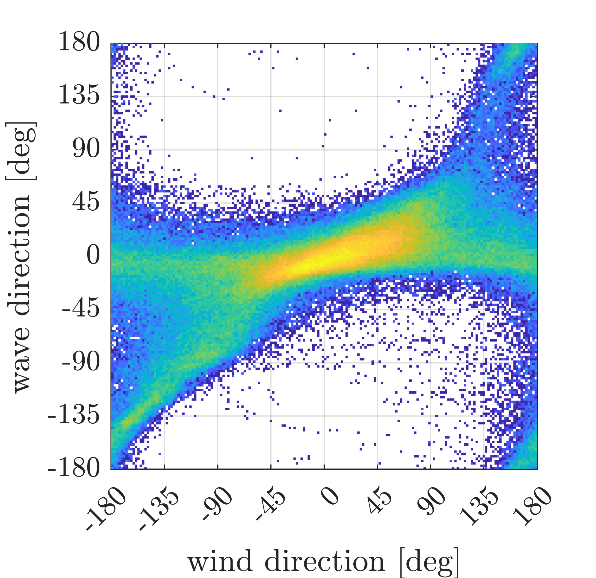
Figure 3: Empirical joint density of wind direction and wave direction.

To assess the variation in the density of angles around a circle, we could plot the number of observations within discrete angular ranges as a histogram. In higher dimensions, visualisation becomes more difficult, but a similar approach can be taken. We count the number of observations within a small angular range of a pseudo-regularly spaced grid of points on the sphere. It is not possible to define evenly-spaced points on the surface of a (hyper) sphere in three or more dimensions. To address this issue, we take the approach proposed in [3], and define a regular grid of points on the $L^{1}$ sphere and project this onto the surface of the $L^{2}$ sphere. This is computed by creating a regular grid of points in the cube $[-1,1]^{d}$, with $2m+1$ points along each dimension: $U_{grid}=\{(i_{1}/m,...,i_{d}/m):i_{j}\in\{-m,...,m\},j=1,...,d\}$. Then, we define $U_{1}=\{\mathbf{u}\in U_{grid}:\|\mathbf{u}\|_{1}=1\}$, where $\|\cdot\|_{1}$ is the $L^{1}$ norm given by $\|(u_{1},...,u_{d})\|_{1}=|u_{1}|+\cdots+|u_{d}|$. Finally, we compute a set of direction vectors $U\subset\mathbb{S}^{d-1}$ by $U=\{\mathbf{u}/\|\mathbf{u}\|_{2}:\mathbf{u}\in U_{1}\}$. This is illustrated in Figure 4 for the case $m=5$ and $d=3$.

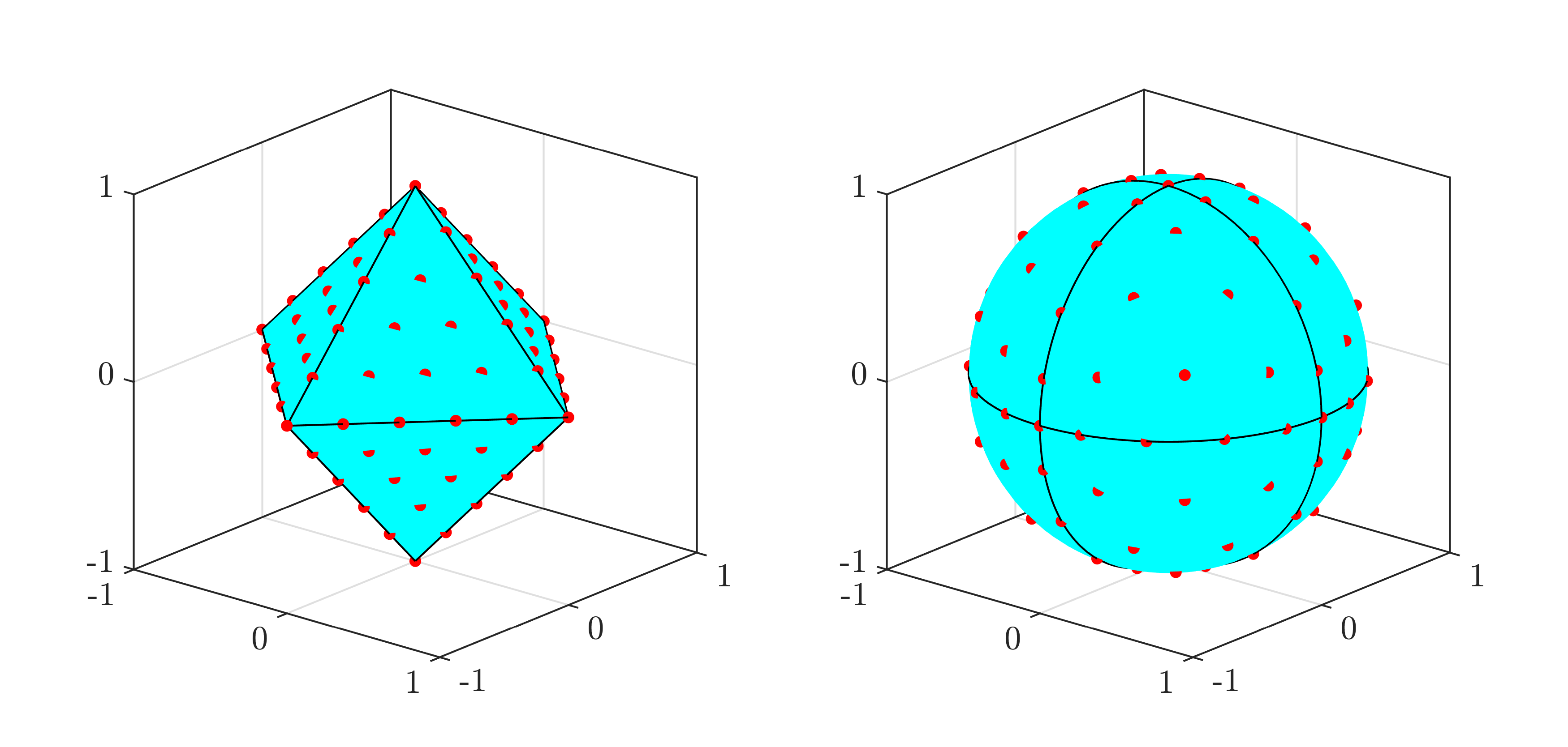
Figure 4: Illustration of the mapping of regularly spaced vectors on the surface of the $L^{1}$ unit sphere (left) onto the $L^{2}$ unit sphere (right).

The dot product of two unit vectors is the cosine of the angle between them. Therefore, for each $\mathbf{u}_{j}\in U$ we count the number of observed angles with $\arccos(\mathbf{w}_{i}\cdot\mathbf{u}_{j})<\theta_{max}$, where $\theta_{max}$ is some prescribed range. Although there may be some overlap between the ranges defined above, this analysis still gives an indication of how the density of angles varies over the sphere.

Figure 6 shows the empirical CDF of the number of observations in a cell chosen at random, for a cell radius of $\theta_{max}=15^{\circ}$ and a set of 1002 direction vectors (generated using $m=5$ in the definition of $U_{grid}$ above). One feature that is evident is that over 50% of angular cells contain no observations. This is due to the particular choice of origin, which was selected to meet the assumption of a star-shaped distribution. Figure 6 also shows the number of observations in each of the 32 orthants in $\mathbb{R}^{5}$ (an orthant is the $d$-dimensional analogue of a quadrant of the plane). There are five orthants which contain no observations, and a further five which contain fewer than 100 observations (out of a total of 271,704 observations). The SPAR model estimates of the extremes in these regions will therefore be highly uncertain in the orthants with little data. However, Figure 6 shows scatter plots of the maximum observed values of $H_{s}$ and $U_{10}$ in each of the 1002 angular cells against the corresponding number of observations in the cell, indicating that larger values of these variables tend to coincide with higher angular densities. The higher uncertainties associated with the lower occurrence regions should therefore have less effect on the global extremes.

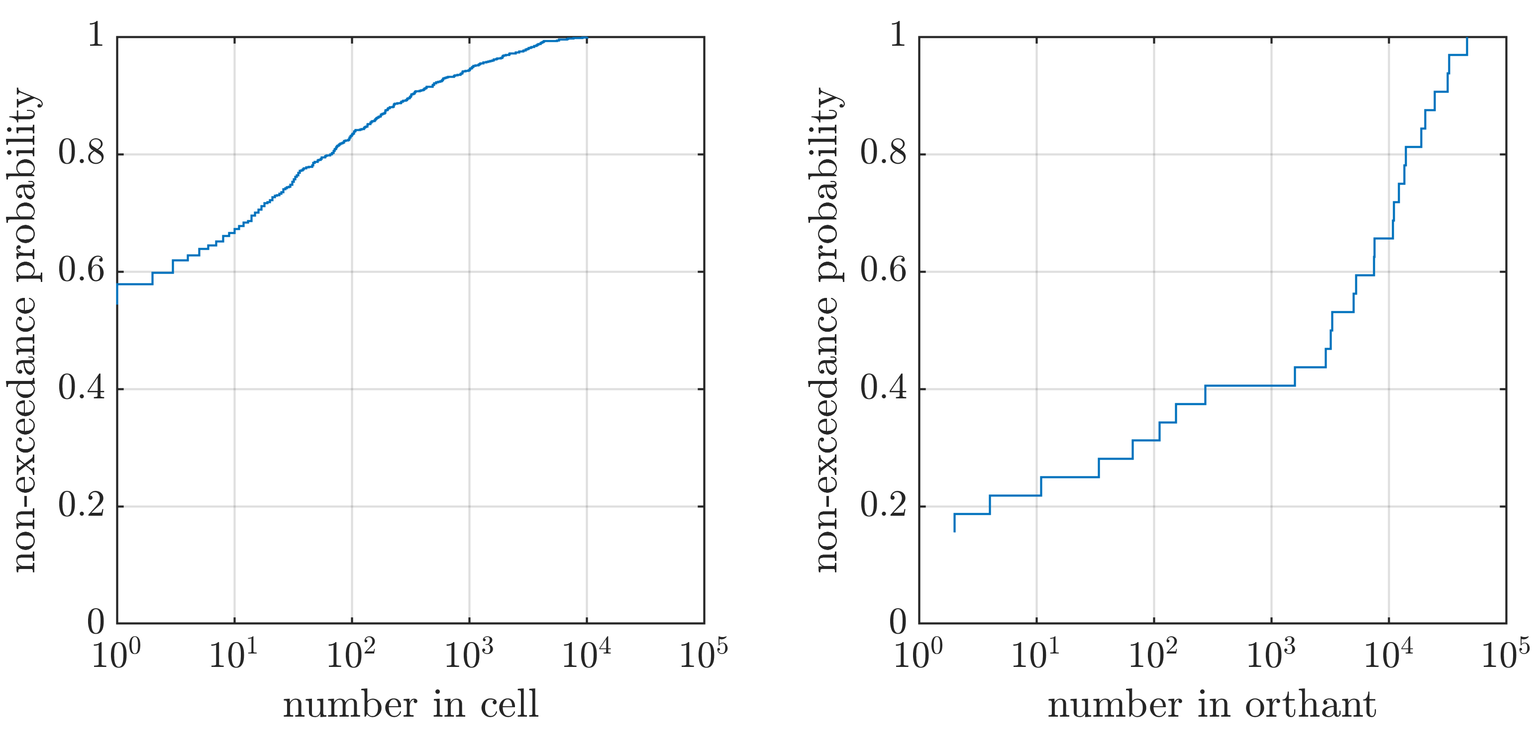
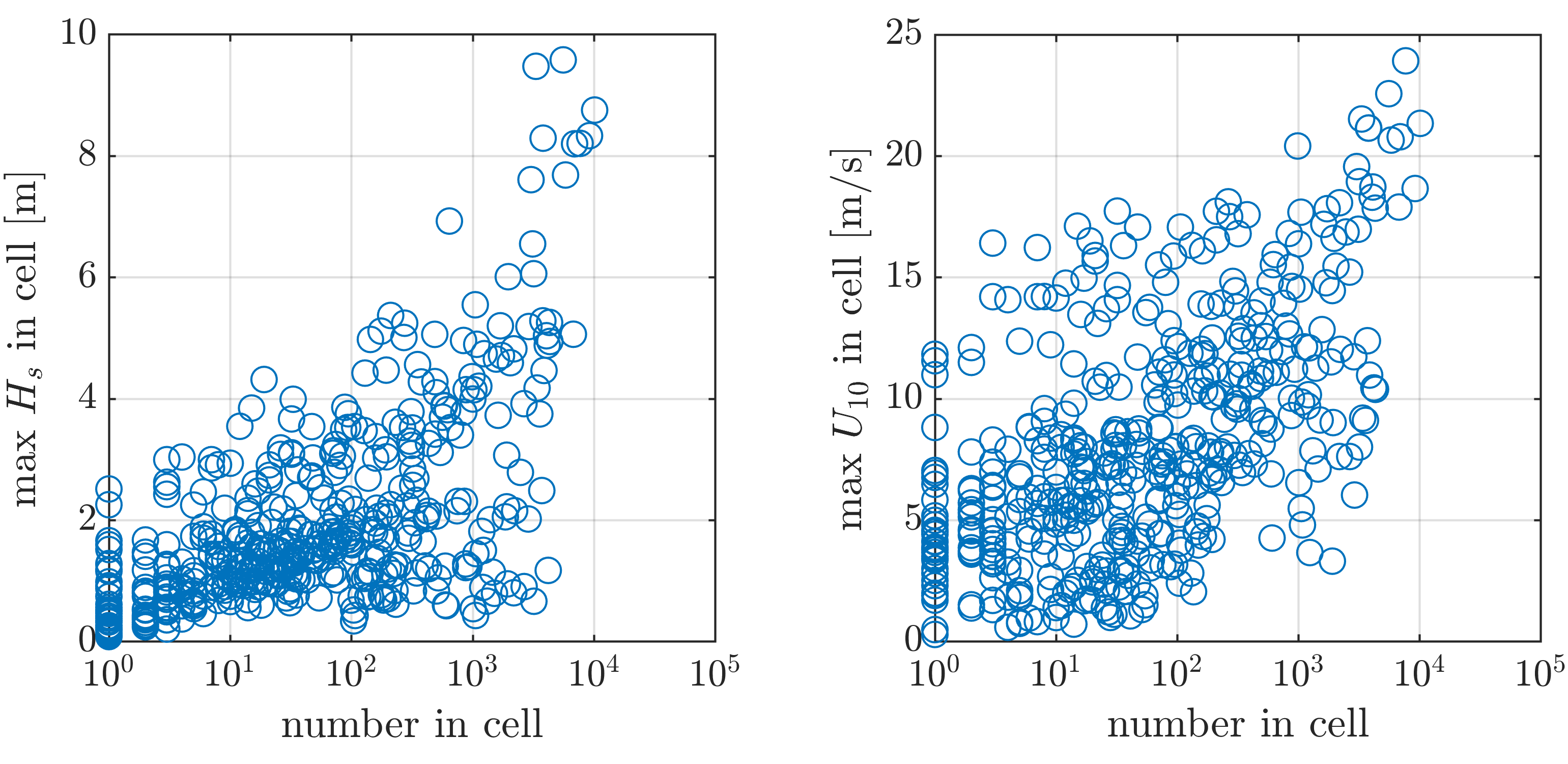
Figure 5: Left: Empirical distribution of the number of points within a $15^{\circ}$ radius of each direction vector. Right: empirical distribution of the number of points in each of the 32 orthants of $\mathbb{R}^{5}$.

Figure 6: Maximum observed $H_{s}$ and $U_{10}$ in each local angular cell vs. number in cell.

Figure 8 shows a scatter plot of $T_{m}$ against $H_{x}$ and $H_{y}$. (A plot of the normalised variables $(X_{3},X_{4},X_{5})$ would look similar, but the non-normalised variables are shown here to aid physical interpretation). The conical shaped bound imposed by the limiting wave steepness is evident. Another feature that is apparent is that the data cloud is hollow on the side $H_{x}<0$. This is because of fetch limitations in this direction, meaning that waves propagating towards the west are steeper wind-driven waves, so that $H_{s}$ and $T_{m}$ are strongly correlated in this region. This violates the assumption of the distribution being star-shaped with respect to the choice of origin. However, the ‘edge region’ that is not modelled corresponds to low values of $H_{s}$ at a given $T_{m}$ and wave direction, which is less critical for extreme responses.

For the present choice of origin at $(H_{x},H_{y},T_{m})=(0,0,6.2)$, it appears that there are some sharp changes in the distribution with the vertical angle, for rays towards the negative x direction. This might be hard to capture with an ANN. Nevertheless, we can assess how well the model performs, given these challenges.

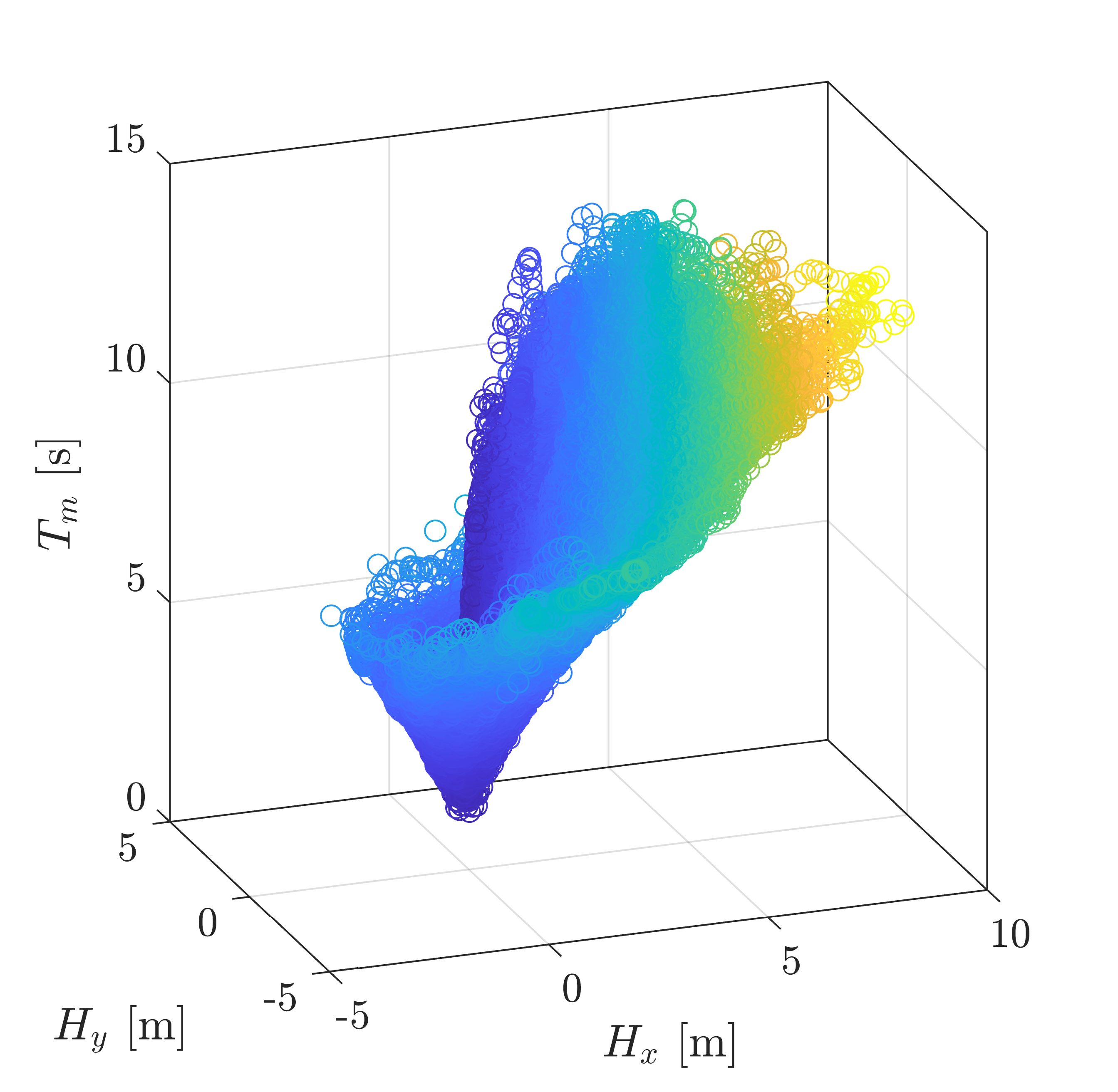
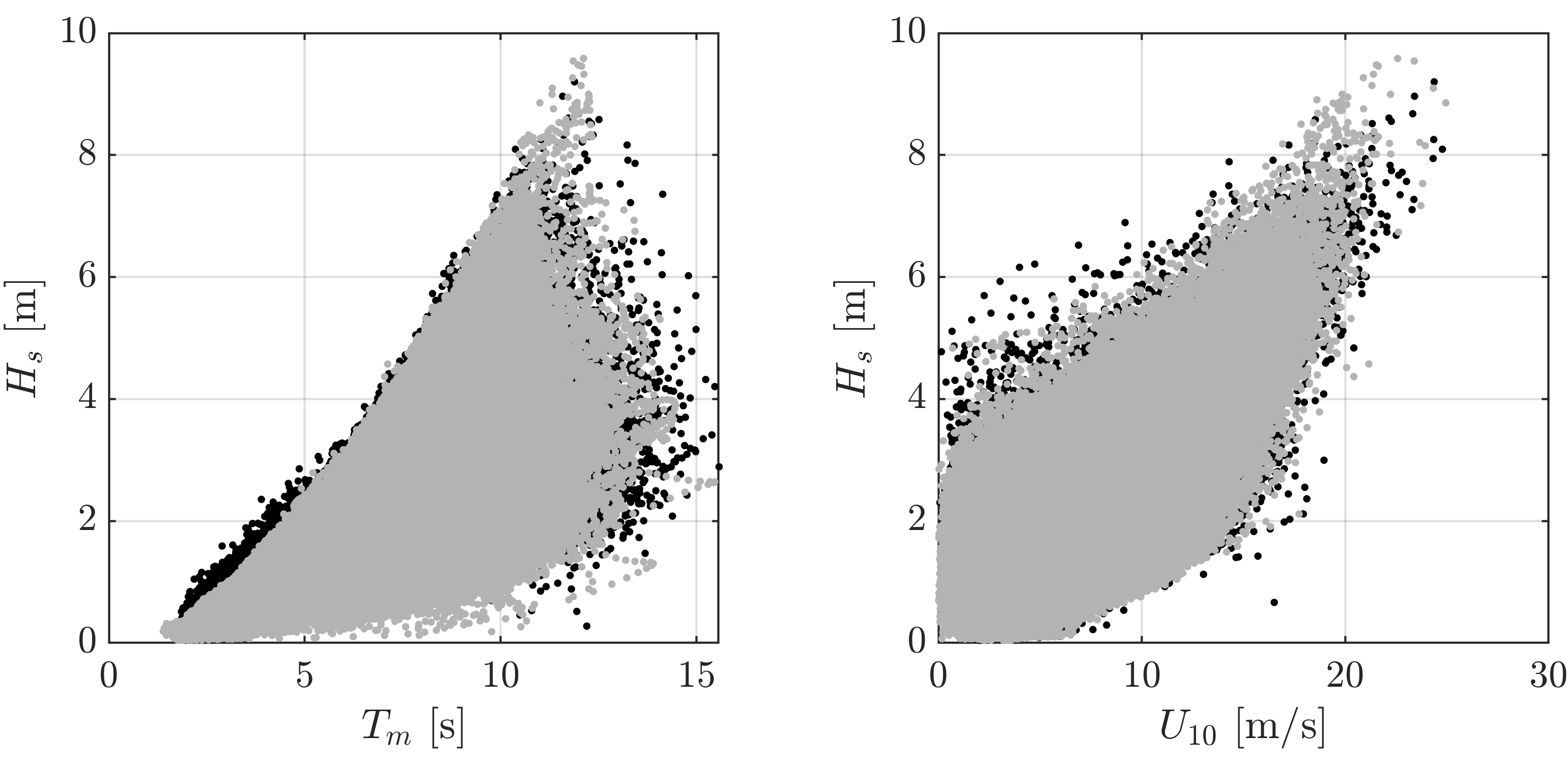
Figure 7: Scatter plot of observations of x-y components of $H_{s}$ and $T_{m}$. Colour indicates value of $H_{s}=\sqrt{H_{x}^{2}+H_{y}^{2}}$ (blue=low, yellow=high).

Figure 8: Scatter plots of pairwise relations between simulated (black) and observed (grey) data in original variable space.

4.4 Diagnostic plots

Creating diagnostic plots to assess goodness-of-fit is challenging in multivariate problems. Assessing pairwise relations, as described above, is one option, where observed and simulated data can be overlaid to visually assess the plausibility of the fitted model, as shown in Figure 2, where the simulated sample from the fitted SPAR model is of equal size to the observed sample. Overall, the simulated relationships between variables closely follow those of the observations. Figure 8 shows scatter plots of the data transformed back to the original scale, to assess the modelled relationship between $H_{s}$, $T_{m},$ and $U_{10}$. Again, the simulated data is a good representation of the observations. The model predicts some larger values of steep waves than observed. However, these occur at lower wave heights, so are less critical for design purposes.

As the SPAR model does not model the tails of the marginal variable directly, it is also useful to assess how well the simulated data matches the observed marginal tails. Quantile-quantile (QQ) plots of the observed and simulated marginal variables are shown along the diagonal in Figure 2. The agreement appears good. However, it is difficult to assess the quality of fit on this scale. Instead, Figure 9 shows exceedance and non-exceedance probabilities on a logarithmic scale for the five variables used in the model, as well as the derived variables $H_{s}$, $U_{10},$ and $s$. Overall, the model performs well and provides a good match for both the upper and lower observed tails. There is a slight tendency to underestimate the upper tail of $H_{x}$, which results in a slight underestimation of the upper tail of $H_{s}$. The over-prediction of steep waves mentioned above is also evident.

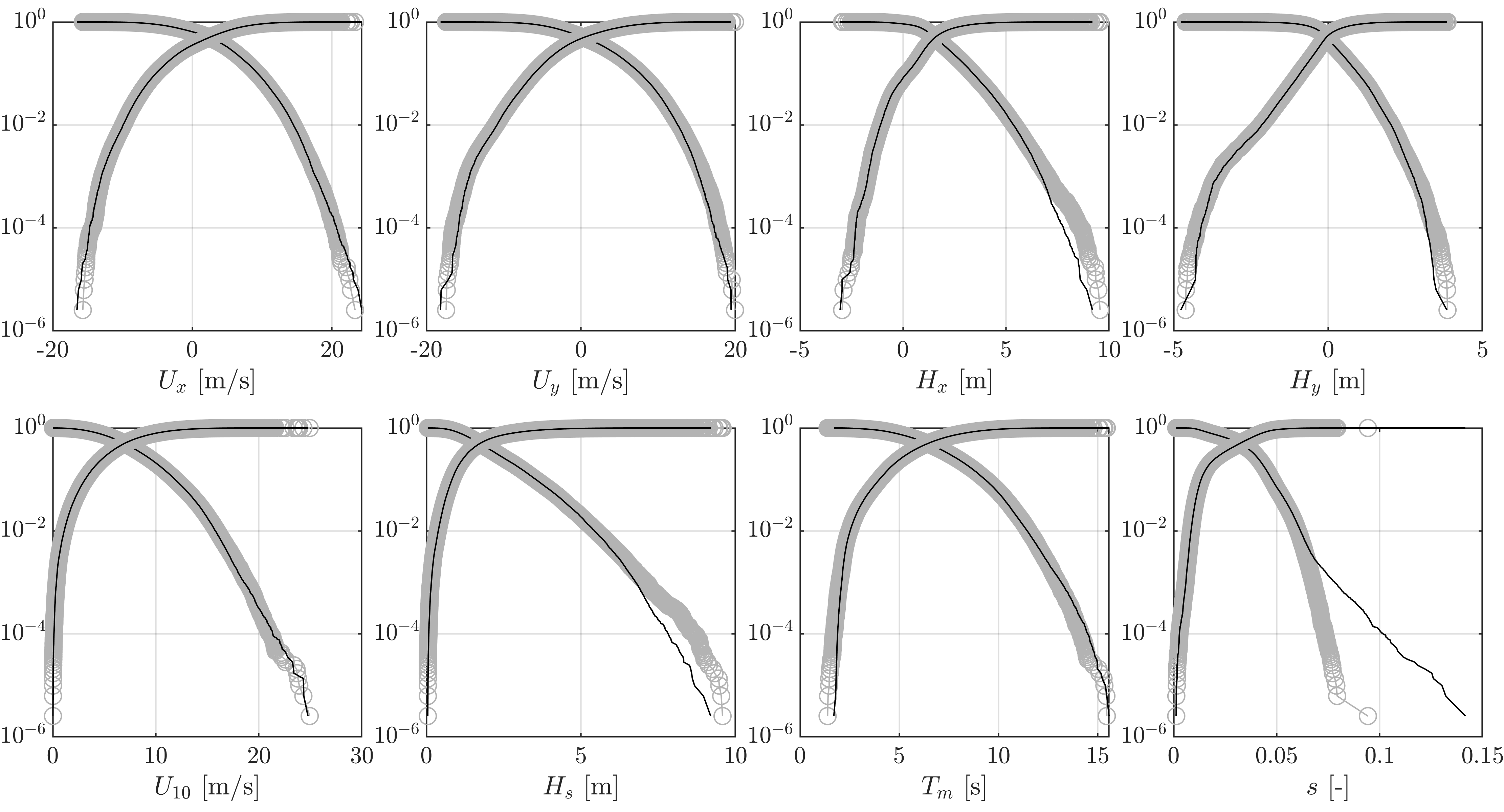
Figure 9: Exceedance and non-exceedance probabilities of marginal and related variables for observed (grey circles) and simulated (black lines) data.

Finally, to give an indication of the variation in model performance over the angular domain, Figure 10 shows QQ plots of simulated against observed threshold exceedances, binned over small angular ranges. As above, we have used a grid of 1002 fixed angles and a radius of $15^{\circ}$ to define the angular bins. Only bins with 200 or more observations have been used, so that there are approximately 20 or more threshold exceedances per bin. The local threshold is taken as the average of the empirical 90th percentile of observed and simulated values in each bin (this approximates an average of the non-stationary threshold over the bin). There is some scatter between the observed and simulated values. However, the aggregated trend shows good agreement, although with a slight tendency to underestimate at larger values. This may be related to the use of maximum likelihood estimation, which is known to produce a slight negative bias in quantile estimates for small sample sizes [57].

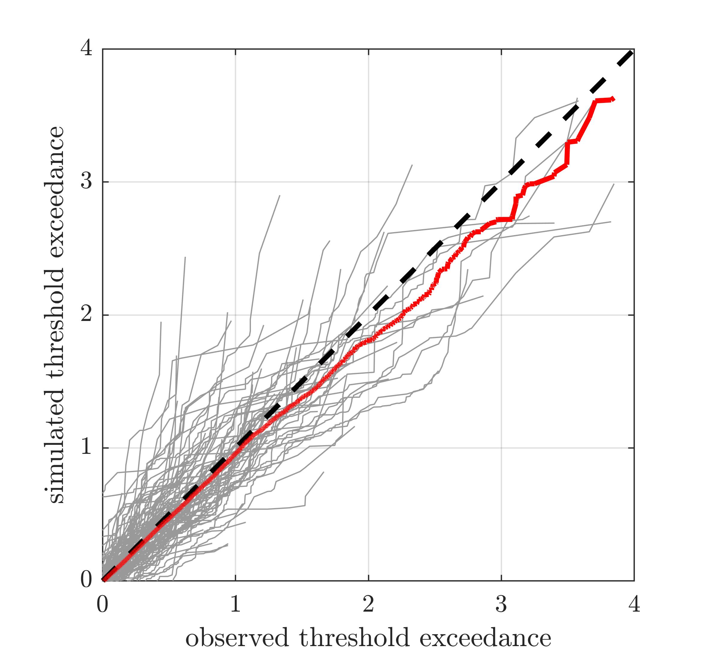
Figure 10: QQ plots of simulated vs observed threshold exceedances in bins of $15^{\circ}$ radius from a grid of points on $\mathbb{S}^{4}$. Grey lines are individual bins; red line is aggregated value over all bins; black dashed line is equality.

5 Discussion and conclusions

In this work, we have introduced a deep learning framework for inference with the SPAR model. The computational scalability and robustness of neural networks result in a modelling approach which requires very few assumptions, offers a high degree of flexibility, and can be applied in higher-dimensional settings compared to existing techniques. We use our approach to approximate the complex joint tail behaviour of a five dimensional metocean dataset, with diagnostics indicating our model is able to accurately represent the observed dependence structure. Given the complex dependence structures observed in the data, the MLP model for the angular variation of the GP parameters performs very well in representing the ‘extremes’ of the dataset. By ‘extremes’, we are referring not just to the largest and smallest values of each observed variable, but anywhere on the outer part of the data cloud. Moreover, the SPAR model provides an asymptotically justified basis for extrapolating outside the range of observations. Simulation from the fitted SPAR model subsequently allows ones to generate large, physically-realistic event sets, allowing practitioners to easily perform robust risk assessments and estimate probabilities of structural failure.

We note that selecting an architecture for any neural network is non-trivial, and care must be taken to ensure the resulting model offers sufficient flexibility without overfitting. We also remark that, in general, neural networks require a large amount of data for accurate model fitting [50]; this is generally a challenge for modelling extremes since, by definition, very little data are available. It is currently not clear what sample sizes, tuning parameters, or architectures are required to accurately fit the SPAR model via deep learning, and this should be explored in further work. In the present approach, we have used 80% of the data for training and 20% for validation. The validation data are used to avoid overfitting. It is possible that using only 20% of observations for validation is insufficient to force a sufficiently smooth solution in regions of sparse angular observations. An alternative is to use a full cross-validation scheme, in which the model results are averaged over e.g., five fits using a different 20% of the data for testing. This would make better use of the limited observations, although with increased computational cost.

One notable observation from Section 4 was that the choice of origin for defining the SPAR model was non-trivial. Initially, we naively assumed that the componentwise mean was a suitable origin, but this resulted in issues when fitting the model, as the data cloud was not star-shaped with respect to this initial choice of origin. Selecting an appropriate origin for the SPAR model beyond the lower dimensional ($d\leq 3$) setting remains a challenge as full data visualisation is not possible, and inappropriate choices can invalidate the modelling assumptions. Future work could explore the robust selection of the origin in a data-driven manner, removing the need for domain specific knowledge.

From Section 4, it was also clear that as the dimension of the data increases, so too does the sparsity. This is particularly apparent in Figure 6, where we observed some orthants containing just a handful of observations. Inference within such regions is problematic, since there is very little data to train the neural network model. We also noted that in sparse regions, the resulting parameter estimates did not always respect the physical features of the data, e.g., upper bounds of the variables. Such issues are not unique to the SPAR model, and one would expect to encounter the same problems with alternative modelling approaches when applied in high dimensions. Future work could explore whether notions of sparsity can be incorporated into the SPAR framework to improve the robustness and efficiency of the model.

References

- [1] Sverre Haver and Steven R Winterstein “Environmental contour lines: A method for estimating long term extremes by a short term analysis” In SNAME Maritime Convention, 2008, pp. D011S002R005 DOI: 10.5957/SMC-2008-067
- [2] Quentin Derbanne and Guillaume de Hauteclocque “A new approach for environmental contour and multivariate de-clustering” In 38th International Conference on Ocean, Offshore and Arctic Engineering, 2019, pp. OMAE2019/95993 DOI: 10.1115/OMAE2019-95993
- [3] Ed Mackay and Guillaume Hauteclocque “Model-free environmental contours in higher dimensions” In Ocean Engineering 273, 2023, pp. 113959 DOI: 10.1016/j.oceaneng.2023.113959
- [4] Andreas F Haselsteiner et al. “Long-term extreme response of an offshore turbine: how accurate are contour-based estimates?” In Renewable Energy 181, 2022, pp. 945–965 DOI: 10.1016/j.renene.2021.09.077
- [5] Matthew Speers, David Randell, Jonathan Tawn and Philip Jonathan “Estimating Metocean Environments Associated with Extreme Structural Response” In Ocean Engineering 311, 2024, pp. 118754 DOI: 10.1016/j.oceaneng.2024.118754
- [6] Emma Ross et al. “On environmental contours for marine and coastal design” In Ocean Engineering 195, 2020, pp. 106194 DOI: 10.1016/j.oceaneng.2019.106194
- [7] Andreas F Haselsteiner et al. “A benchmarking exercise for environmental contours” In Ocean Engineering 236, 2021, pp. 109504 DOI: 10.1016/j.oceaneng.2021.109504
- [8] Elzbieta M Bitner-Gregersen “Joint met-ocean description for design and operations of marine structures” In Applied Ocean Research 51, 2015, pp. 279–292 DOI: 10.1016/j.apor.2015.01.007
- [9] Jan-Tore Horn et al. “A new combination of conditional environmental distributions” In Applied Ocean Research 73, 2018, pp. 17–26 DOI: 10.1016/j.apor.2018.01.010
- [10] Zhengshun Cheng, Erik Svangstu, Torgeir Moan and Zhen Gao “Long-term joint distribution of environmental conditions in a Norwegian fjord for design of floating bridges” In Ocean Engineering 191, 2019, pp. 106472 DOI: 10.1016/j.oceaneng.2019.106472
- [11] Guillaume de Hauteclocque, Ed Mackay and Erik Vanem “Quantitative comparison of environmental contour approaches” In Ocean Engineering 245, 2022, pp. 110374 DOI: 10.1016/j.oceaneng.2021.110374
- [12] Harry Joe “Dependence modeling with copulas” In Dependence Modeling with Copulas CRC Press, 2015, pp. 1–457
- [13] J Beirlant, Y Goegebeur, J Segers and J Teugels “Statistics of extremes: theory and applications” Wiley, Chichester, UK, 2004
- [14] Anthony W. Ledford and Jonathan A. Tawn “Modelling dependence within joint tail regions” In Journal of the Royal Statistical Society . Series B ( Methodological ) 59.2, 1997, pp. 475–499 DOI: 10.1111/1467-9868.00080
- [15] J.. Wadsworth and J.. Tawn “A new representation for multivariate tail probabilities” In Bernoulli 19.5 B, 2013, pp. 2689–2714 DOI: 10.3150/12-BEJ471
- [16] Raphaël Huser, Thomas Opitz and Jennifer Wadsworth “Modeling of spatial extremes in environmental data science: Time to move away from max-stable processes” In arXiv preprint arXiv:2401.17430, 2024
- [17] J E Heffernan and J A Tawn “A conditional approach for multivariate extreme values” In Journal of the Royal Statistical Society. Series B (Methodology) 66, 2004, pp. 497–546 DOI: 10.1111/j.1467-9868.2004.02050.x
- [18] Y. Liu and J.. Tawn “Self-consistent estimation of conditional multivariate extreme value distributions” In Journal of Multivariate Analysis 127 Elsevier Inc., 2014, pp. 19–35 DOI: 10.1016/j.jmva.2014.02.003
- [19] Ross Towe et al. “Estimation of associated values from conditional extreme value models” In Ocean Engineering 272 Elsevier, 2023, pp. 113808
- [20] Ed Mackay “Improved Models for Multivariate Metocean Extremes”, 2022 URL: https://supergen-ore.net/uploads/resources/IMEX_final_project_summary.pdf
- [21] Ed Mackay and Philip Jonathan “Modelling multivariate extremes through angular-radial decomposition of the density function” In arXiv preprint arXiv:2310.12711, 2023
- [22] Callum John Rowlandson Murphy-Barltrop, Ed Mackay and Philip Jonathan “Inference for bivariate extremes via a semi-parametric angular-radial model” In Extremes, 2024, pp. 1–30 DOI: 10.1007/s10687-024-00492-2
- [23] EBL Mackay, CJR Murphy-Barltrop and Philip Jonathan “The SPAR Model: A New Paradigm for Multivariate Extremes. Application to Joint Distributions of Metocean Variables” In Journal of Offshore Mechanics and Arctic Engineering 147.1, 2025, pp. 011205 DOI: 10.1115/1.4065968
- [24] Stuart Coles “An Introduction to Statistical Modeling of Extreme Values” Springer, 2001 DOI: 10.1198/tech.2002.s73
- [25] Ed Mackay and Andreas F Haselsteiner “Marginal and total exceedance probabilities of environmental contours” In Marine Structures 75, 2021, pp. 102863 DOI: 10.1016/j.marstruc.2020.102863
- [26] Kanti V Mardia and Peter E Jupp “Directional Statistics” John Wiley & Sons, 2000
- [27] Christophe Ley and Thomas Verdebout “Modern Directional Statistics” ChapmanHall/CRC, 2017 DOI: 10.1201/9781315119472
- [28] Arthur Pewsey and Eduardo García-Portugués “Recent advances in directional statistics” In TEST 30, 2021, pp. 1–58 DOI: 10.1007/s11749-021-00759-x
- [29] Peter Hall, GS Watson and Javier Cabrera “Kernel density estimation with spherical data” In Biometrika 74.4, 1987, pp. 751–762 DOI: 10.1093/biomet/74.4.751
- [30] ZD Bai, C Radhakrishna Rao and LC Zhao “Kernel estimators of density function of directional data” In Multivariate statistics and probability Elsevier, 1989, pp. 24–39 DOI: 10.1016/B978-0-12-580205-5.50008-2
- [31] Jennifer A Mooney, Peter J Helms and Ian T Jolliffe “Fitting mixtures of von Mises distributions: a case study involving sudden infant death syndrome” In Computational Statistics & Data Analysis 41.3-4, 2003, pp. 505–513 DOI: 10.1016/S0167-9473(02)00181-0
- [32] Yuejiao Fu, Jiahua Chen and Pengfei Li “Modified likelihood ratio test for homogeneity in a mixture of von Mises distributions” In Journal of Statistical Planning and Inference 138.3, 2008, pp. 667–681 DOI: 10.1016/j.jspi.2007.01.003
- [33] José TAS Ferreira, Miguel A Juárez and Mark FJ Steel “Directional log-spline distributions” In Bayesian Analysis 3, 2008, pp. 297–316 DOI: 10.1214/08-BA311
- [34] Kurt Hornik and Bettina Grün “movMF: An R package for fitting mixtures of von Mises-Fisher distributions.” In Journal of Statistical Software 58.10, 2014, pp. 1–31 DOI: 10.18637/jss.v058.i10
- [35] Valérie Chavez-Demoulin and Anthony C Davison “Generalized additive modelling of sample extremes” In Journal of the Royal Statistical Society Series C: Applied Statistics 54.1, 2005, pp. 207–222 DOI: 10.1111/j.1467-9876.2005.00479.x
- [36] D. Randell, K. Turnbull, K. Ewans and P. Jonathan “Bayesian inference for nonstationary marginal extremes” In Environmetrics 27.7, 2016, pp. 439–450 DOI: 10.1002/ENV.2403
- [37] Benjamin D. Youngman “Generalized Additive Models for Exceedances of High Thresholds With an Application to Return Level Estimation for U.S. Wind Gusts” In Journal of the American Statistical Association 114.528, 2019, pp. 1865–1879 DOI: 10.1080/01621459.2018.1529596
- [38] E. Zanini et al. “Flexible covariate representations for extremes” In Environmetrics 31, 2020, pp. e2624 DOI: 10.1002/env.2624
- [39] Anna Maria Barlow, Ed Mackay, Emma Eastoe and Philip Jonathan “A penalised piecewise-linear model for non-stationary extreme value analysis of peaks over threshold” In Ocean Engineering 267, 2023, pp. 113265 DOI: 10.1016/j.oceaneng.2022.113265
- [40] Emma S Simpson and Jonathan A Tawn “Estimating the limiting shape of bivariate scaled sample clouds: with additional benefits of self-consistent inference for existing extremal dependence properties” In Electronic Journal of Statistics 18.2 The Institute of Mathematical Statisticsthe Bernoulli Society, 2024, pp. 4582–4611
- [41] Reetam Majumder, Benjamin A Shaby, Brian J Reich and Daniel Cooley “Semiparametric Estimation of the Shape of the Limiting Multivariate Point Cloud” In arXiv preprint arXiv:2306.13257, 2023
- [42] J. Richards and R. Huser “Extreme Quantile Regression with Deep Learning” In Handbook on Statistics of Extremes Chapman & Hall / CRC, 2024
- [43] Callum JR Murphy-Barltrop, Reetam Majumder and Jordan Richards “Deep Learning of Multivariate Extremes via a Geometric Representation” In arXiv preprint arXiv:2406.19936, 2024
- [44] Tyler Wilson, Pang-Ning Tan and Lifeng Luo “DeepGPD: A deep learning approach for modeling geospatio-temporal extreme events” In Proceedings of the AAAI Conference on Artificial Intelligence 36.4, 2022, pp. 4245–4253
- [45] Jordan Richards, Raphaël Huser, Emanuele Bevacqua and Jakob Zscheischler “Insights into the drivers and spatiotemporal trends of extreme Mediterranean wildfires with statistical deep learning” In Artificial Intelligence for the Earth Systems 2.4 American Meteorological Society, 2023, pp. e220095
- [46] Daniela Cisneros et al. “Deep graphical regression for jointly moderate and extreme Australian wildfires” In Spatial Statistics Elsevier, 2024, pp. 100811
- [47] Olivier C Pasche and Sebastian Engelke “Neural networks for extreme quantile regression with an application to forecasting of flood risk” In The Annals of Applied Statistics 18.4 Institute of Mathematical Statistics, 2024, pp. 2818–2839
- [48] David Roxbee Cox and Nancy Reid “Parameter orthogonality and approximate conditional inference” In Journal of the Royal Statistical Society: Series B (Methodological) 49.1 Wiley Online Library, 1987, pp. 1–18
- [49] Stan Tendijck, David Randell, Graham Feld and Philip Jonathan “Practical non-stationary extreme value analysis of peaks over threshold using the generalised Pareto distribution: Estimating uncertainties in return values” In Ocean Engineering 312, 2024, pp. 119247 DOI: 10.1016/j.oceaneng.2024.119247
- [50] Ian Goodfellow, Yoshua Bengio and Aaron Courville “Deep Learning” MIT press, 2016
- [51] Roger Koenker, Victor Chernozhukov, Xuming He and Limin Peng “Handbook of Quantile Regression” CRC Press, 2017
- [52] R Neuneier, F Hergert, W Finnoff and D Ormoneit “Estimation of conditional densities: A comparison of neural network approaches” In Proceedings of the International Conference on Artificial Neural Networks, 1994, 1994, pp. 689–692 Springer
- [53] Jonas Rothfuss, Fabio Ferreira, Simon Walther and Maxim Ulrich “Conditional density estimation with neural networks: Best practices and benchmarks” In arXiv preprint arXiv:1903.00954, 2019
- [54] Diederik P Kingma and Jimmy Ba “Adam: A method for stochastic optimization” In arXiv preprint arXiv:1412.6980, 2014
- [55] Jordan Richards and Raphaël Huser “Regression modelling of spatiotemporal extreme US wildfires via partially-interpretable neural networks” In arXiv preprint arXiv:2208.07581, 2022
- [56] Guillermo Hansen, Irmina Herburt, Horst Martini and Maria Moszyńska “Starshaped sets” In Aequationes mathematicae 94, 2020, pp. 1001–1092 DOI: 10.1007/s00010-020-00720-7
- [57] Jonathan RM Hosking and James R Wallis “Parameter and quantile estimation for the generalized Pareto distribution” In Technometrics 29.3 Taylor & Francis, 1987, pp. 339–349