Debiasing of Two-Line Element Sets for Batch Least Squares Pseudo-Orbit Determination in MEO and GEO

Abstract

The availability of accurate and timely state predictions for objects in near-Earth orbits is becoming increasingly important due to the growing congestion in key orbital regimes. The TLE catalogue remains, to this day, one of the few publicly-available, comprehensive sources of near-Earth object ephemerides. At the same time, TLE are affected by measurement noise and are limited by the low accuracy of the SGP4 theory, introducing significant uncertainty into state predictions. Previous literature has shown that filtering TLE with batch least squares methods can yield significant improvements in long-term state prediction accuracy. However, this process can be highly sensitive to TLE quality which can vary throughout the year. In this study, it is shown that either extended-duration fit windows of the order of months, or the removal of systematic biases in along-track position prior to state estimation can produce significant reductions in post-fit position errors. Simple models for estimating these systematic biases are shown to be effective without introducing the need for high-complexity ML models. Furthermore, by establishing a TLE-based error metric, the need for high accuracy ephemerides is removed when creating these models. For selected satellites in the MEO regime, post-fit position errors are reduced by up to $80\text{\,}\%$, from approximately $5\text{\,}\mathrm{km}1\text{\,}\mathrm{km}$; meanwhile, for selected satellites in the GEO/GSO regime, large oscillations in post-fit position error can be suppressed.

TLE short = TLE, long = Two-Line Element Set S-TLE short = S-TLE, long = Synthetic Two-Line Element Set JPL short = JPL, long = Jet Propulsion Laboratory ESA short = ESA, long = European Space Agency ESA_Imperial short = ESA, long = Early Stage Assessment LSR short = LSR, long = Late Stage Review NASA short = NASA, long = National Aeronautics and Space Administration IoS short = IoS, long = Interruption of Studies PA short = PA, long = Polynomial Algebra PAMC short = PAMC, long = Polynomial Algebra Monte Carlo UQ short = UQ, long = Uncertainty Quantification LEO short = LEO, long = Low Earth Orbit MEO short = MEO, long = Medium Earth Orbit GEO short = GEO, long = Geostationary Earth Orbit GSO short = GSO, long = Geosynchronous Earth Orbit EqOE short = EqOE, long = Equinoctial Orbital Element GEqOE short = GEqOE, long = Generalised Equinoctial Orbital Element AEqOE short = AEqOE, long = Alternate Equinoctial Orbital Element J2EqOE short = J₂EqOE, long = J₂ Equinoctial Orbital Element GPS short = GPS, long = Global Positioning System GNSS short = GNSS, long = Global Navigation Satellite System WAAS short = WAAS, long = Wide Area Augementation System CDDIS short = CDDIS, long = Crustal Dynamics Data Information System KF short = KF, long = Kalman Filter EKF short = EKF, long = Extended Kalman Filter UKF short = UKF, long = Unscented Kalman Filter DA short = DA, long = Differential Algebra CPU short = CPU, long = Central Processing Unit GPU short = GPU, long = Graphics Processing Unit SRP short = SRP, long = Solar Radiation Pressure STM short = STM, long = State Transition Matrix, long-plural-form = State Transition Matrices RTN short = RTN, long = Radial, Transverse, Normal, tag = abbrev GP short = GP, long = General Perturbation, tag = abbrev SP short = SP, long = Special Perturbation, tag = abbrev SSA short = SSA, long = Space Situational Awareness, tag = abbrev SDA short = SDA, long = Space Domain Awareness, tag = abbrev USSF short = USSF, long = United States Space Force, tag = abbrev CDM short = CDM, long = Conjunction Data Message, tag = abbrev NORAD short = NORAD, long = North American Aerospace Defense Command, tag = abbrev ILRS short = ILRS, long = International Lasing Ranging Service, tag = abbrev LAGEOS short = LAGEOS, long = Laser Geodynamics Satellite, SLR short = SLR, long = Satellite Laser Ranging, OD short = OD, long = Orbit Determination, P-OD short = P-OD, long = Pseudo-Orbit Determination, EoM short = EoM, long = Equation of Motion, long-plural-form = Equations of Motion XML short = XML, long = Extensible Markup Language KVN short = KVN, long = Key-value Notation JSON short = JSON, long = JavaScript Object Notation RSO short = RSO, long = Resident Space Object UT short = UT, long = Unscented Transform CA short = CA, long = Conjunction Assessment RMSE short = RMSE, long = Root-Mean-Square Error ML short = ML, long = Machine Learning LSODAR short = LSODAR, long = Livermore Solver for Ordinary Differential Equations with Automatic Method Switching for Stiff and Non-stiff Problems and with Root-finding, TEME short = TEME, long = True Equator Mean Equinox, GCRF short = GCRF, long = Geocentric Celestial Reference Frame, IVP short = IVP, long = Initial Value Problem,

[1]organization=Imperial College London, addressline=Exhibition Road, city=London, postcode=SW7 2AZ, country=United Kingdom

1 Introduction

The rise of the “New Space” era, driven by the growth in the number of commercial actors in the space domain, has led to a significant increase in the near-Earth RSO population over the past decade, including year-on-year growth in the number of launches and payloads (ESA, 2023).

The growth in the RSO population has been seen primarily in the LEO and GEO regimes, therefore the majority of these objects are concentrated into the same limited regions. The risk of collisions between RSO continues to grow, highlighting the importance of improving the capacity and capabilities of CA systems. These are highly dependent on accurate and precise state estimates to remain effective. With future exploration and development, the cislunar environment will become increasingly relevant, underscoring the need to understand various different orbital regimes.

Many operators have high precision state estimates for their own spacecraft based on their own on-board sensors, however they remain dependent on governmental and commercial SSA organisations, and data sharing with other operators, for state estimates of other objects. The financial cost of these services mean that smaller operators and academia remain reliant on publicly available sources, primarily TLE published by the USSF.

One of the greatest advantages of TLE is that they are freely available for a significant proportion of RSO currently (and formerly) in near-Earth orbit. They represent an unparalleled source of data for RSO state vectors. Nevertheless, they are subject to a number of limitations which are difficult to overcome, primarily their limited accuracy when predicting states. This is due to the analytical models used by the format (SGP4 and SDP4, now commonly referred to jointly as SGP4) which use simplified perturbation models with limited fidelity (Hoots et al., 2004). This is despite the fact that TLE themselves are generated by fitting the models to higher-order predictions made by direct OD (Hejduk et al., 2013). Additionally, the lack of uncertainty information for TLE mean that their accuracy, even at epoch, remains effectively unknown. The result is a widely used data format with high availability across the orbital catalogue but with unknown or poor accuracy, making them unsuitable for precision applications.

The limited fidelity of the SGP4 model was identified as an issue as TLE became more widely used, particularly when considering “the requirements and problems in modern space mission operations” (Conkey & Zielinski, 2022). For example, the stringent requirements on accuracy for CA remain unsatisfied by traditional TLE which are only sufficient for “providing a first-order screening for collision alerting” (Chao & Hoots, 2018). The limitations of traditional TLE and SGP4 led to the development of the SGP4-XP model, a new algorithm for propagating TLE with greater precision, albeit with a reduction in computational performance (Conkey & Zielinski, 2022). An extension of SGP4, this updated model includes improved geopotential and resonance modelling, higher order lunisolar perturbations, a more detailed atmospheric model, and improved SRP modelling (Conkey & Zielinski, 2022; Payne et al., 2022; Holincheck & Cathell, 2021). It should be noted that TLE using SGP4-XP, designated as Type 4 ephemerides, are not compatible with the original SGP4 model, nor vice versa (Conkey & Zielinski, 2022). This is a product of the models being based on different averaging theories and, hence, they correspond to different dynamical systems.

Binaries for SGP4-XP are available from USSF; however, mean elements compatible with the SGP4-XP theory have not been publicly distributed as of the date of writing. Nevertheless, testing with synthetically generated Type 4 TLE has demonstrated significant improvements in prediction accuracy for objects in the MEO and GEO/GSO regimes (Conkey & Zielinski, 2022). One feature, particularly critical for P-OD, is the “more realistic dynamics coming from the SGP4-XP algorithm [yielding] a structure in the error which is more Gaussian than that of the classical SGP4” (Conkey & Zielinski, 2022). This includes a significant reduction in along-track error (Payne et al., 2022) which is the primary component of classical TLE error. Since Type 4 TLE remain unavailable publicly, methods for reducing TLE biases remain an important area of investigation for deriving higher precision ephemerides.

Previous literature has demonstrated that it is possible to use TLE in conjunction with higher fidelity orbital propagators to produce more accurate state estimations though P-OD. This is the process of conducting OD on products which themselves are the result of an OD process. Levit & Marshall (2011) conducted batch least squares fitting of a high-fidelity numerical model to TLE pseudo-observations, improving the error rate for position prediction in LEO from approximately $100\text{\,}\mathrm{m}\mathrm{/}\mathrm{d}\mathrm{a}\mathrm{y}3000\text{\,}\mathrm{m}\mathrm{/}\mathrm{d}\mathrm{a}\mathrm{y}$ to $50\text{\,}\mathrm{m}\mathrm{/}\mathrm{d}\mathrm{a}\mathrm{y}200\text{\,}\mathrm{m}\mathrm{/}\mathrm{d}\mathrm{a}\mathrm{y}$. Vallado et al. (2013) extended existing analyses by investigating the influence of different estimation parameters, concluding that uncertainty was largest in the along-track direction and that force model fidelity had a limited impact on results. Bennett et al. (2012) demonstrated that relatively simple bias models can be used to improve TLE-based P-OD when fused with SLR data. Chen & Lin (2023), in a study of P-OD techniques on satellites in LEO, showed that fit prediction accuracy can be improved by restricting sampling to within two orbital periods of each epoch. Ly et al. (2020) investigated using statistical and ML techniques to find corrections for GPS satellite TLE to improve prediction, leading to “improved TLEs accuracy from 5 km to 1.5 km with a 90% confidence level”. This study focused on correcting the along-track error present in TLE with kernel regression techniques which revealed correlation between the error and both the Sun-Earth and Moon-Earth distances.

The objective of this study is to revisit past analyses of P-OD on TLE to confirm whether these methods are still effective in light of changes in TLE behaviour over the past decade and, additionally, to investigate the ideal parameters when using batch least squares for achieving the best possible accuracy. We consider passive satellites, both with and without accurate reference ephemerides, to establish an error metric that is purely TLE-based to enable analysis of any object in the TLE catalogue.

The methodology for conducting P-OD will be discussed in Section 2, followed by a presentation of the results in Section 3, including a discussion of considerations for the further development of bias models. Section 5 will provide a summary of the outcomes of the study and potential avenues for future development.

2 Overview of Pseudo-Orbit Determination

The P-OD process can be split into two main components: fit and prediction. In the first, pseudo-observations generated from a set of TLE are used to estimate the state of the satellite. This is followed by additional propagation in the prediction phase to evaluate the quality of the fit by comparing it against a reference “ground truth” set of states provided by either SLR or TLE. The fit and prediction windows are illustrated in Fig. 1 with key quantities including the fit start and end dates, followed immediately by the prediction window.

Fig. 1: Fit and prediction windows.

2.1 Batch Least Squares

The batch least squares estimator considers the problem of selecting model parameters which minimise the errors between states predicted from the model and a set of observed states. In this case, the model is one which represents the future state of a satellite as a function of initial state, physical parameters of the satellite, and prediction time. The following derivation summarises the method as described by Vallado (2013) and Tapley et al. (2004).

2.1.1 Predictor

The predictor is an IVP where the state of an object can be predicted based on an initial state:

$$\dot{\mathbf{x}}=\mathbf{f}(\mathbf{x},t)\text{,}$$ (1)

$$\mathbf{x}(t_{0})=\mathbf{x}_{0}\text{,}$$ (2)

where $\mathbf{x}$ and $\dot{\mathbf{x}}$ are the state and state derivative, $t$ is time, $\mathbf{f}(\mathbf{x},t)$ is the dynamical model of the predictor, and $t_{0}$ and $\mathbf{x}_{0}$ are the initial time and state respectively.

The state at a future time can be predicted by integrating with respect to time:

$$\mathbf{y}^{*}(t)=\mathbf{x}_{0}+\int_{t_{0}}^{t}\dot{\mathbf{x}}\ dt\text{,}$$ (3)

where $\mathbf{y}^{*}(t)$ is the state at a future time $t$. Alternatively, this can be expressed as the solution of a linear system:

$$\mathbf{y}^{*}(t)=\mathbf{A}(t,t_{0})\mathbf{x}_{0}\text{,}$$ (4)

where $\mathbf{A}(t,t_{0})$ is the partial derivatives matrix which maps between initial and predicted states. The derivatives matrix can be further defined as:

$$\mathbf{A}(t,t_{0})=\mathbf{H}(t)\mathbf{\Phi}(t,t_{0})\text{,}$$ (5)

where $\mathbf{H}(t)$ is the observation matrix at time $t$ which maps from state space to observation space, and $\mathbf{\Phi}(t,t_{0})$ is the STM which maps from the initial state at time $t_{0}$ to the predicted state at time $t$. In this case, the state and observation spaces were the same, therefore the observation matrix was simply identity.

By particularising Eq. 4 for $n$ epochs:

$$\mathbf{y}^{*}(t_{0}) =\mathbf{A}(t_{0},t_{0})\mathbf{x}_{0}\text{,}$$ (6)

$$\mathbf{y}^{*}(t_{1}) =\mathbf{A}(t_{1},t_{0})\mathbf{x}_{0}\text{,}$$

$$\mathbf{y}^{*}(t_{2}) =\mathbf{A}(t_{2},t_{0})\mathbf{x}_{0}\text{,}$$

$$\vdots$$

$$\mathbf{y}^{*}(t_{n}) =\mathbf{A}(t_{n},t_{0})\mathbf{x}_{0}\text{,}$$

the individual linear systems can be concatenated into a single overall linear system:

$$\begin{bmatrix}\left[\mathbf{y}^{*}_{0}\right]\\ \left[\mathbf{y}^{*}_{1}\right]\\ \left[\mathbf{y}^{*}_{2}\right]\\ \vdots\\ \left[\mathbf{y}^{*}_{n}\right]\end{bmatrix}=\begin{bmatrix}\left[\mathbf{A}_{0}\right]\\ \left[\mathbf{A}_{1}\right]\\ \left[\mathbf{A}_{2}\right]\\ \vdots\\ \left[\mathbf{A}_{n}\right]\end{bmatrix}\mathbf{x}_{0}\text{,}$$ (7)

where:

$$\mathbf{y}^{*}_{i}=\mathbf{y}^{*}(t_{i})\text{,}$$ (8)

$$\mathbf{A}_{i}=\mathbf{A}(t_{i},t_{0})\text{.}$$ (9)

The predicted state vectors, therefore, can be expressed as a function of an overall derivatives matrix and the initial state vector:

$$\mathbf{y}^{*}=\mathbf{A}\mathbf{x}_{0}\text{.}$$ (10)

2.1.2 Observer

Object states are represented in TLE by a number of parameters, including a set of mean elements, based on a development from theories by Brouwer and Kozai, among others (Hoots et al., 2004; Chao & Hoots, 2018), and a ballistic coefficient. Propagation of these parameters to future times, and conversion to Cartesian state, is based on the SGP4 single-averaged theory. For orbits with a period greater than $225\text{\,}\mathrm{m}\mathrm{i}\mathrm{n}\mathrm{u}\mathrm{t}\mathrm{e}\mathrm{s}$, deep space perturbations are included to “account for lunar and solar gravitation as well as the resonance effects of Earth tesseral harmonics” (Chao & Hoots, 2018).

Propagation with SGP4 can be expressed as an analytical expression:

$$\mathbf{y}(t)=\mathbf{R}\>\mathbf{g}(\mathbf{z}_{k},t)\text{,}$$ (11)

$$\mathbf{z}(t_{k})=\mathbf{z}_{k}\text{,}$$ (12)

where $\mathbf{y}(t)$ is the TLE state at a future time $t$; $\mathbf{R}$ is the rotation matrix from TEME to GCRF; $\mathbf{g}(\mathbf{z},t)$ represents SGP4; and $t_{k}$ and $\mathbf{z}_{k}$ are the epoch and state of the appropriate TLE respectively, including both the mean elements and ballistic coefficient.

SGP4 conducts propagation in its set of mean elements which are converted then into Cartesian positions and velocities in TEME. These are transformed into GCRF for consistency with the predictor. Both the SGP4 propagation and frame transformations were provided by the Orekit spaceflight library (Maisonobe et al., 2010).

Similar to the predictor, the observations are concatenated into a single column vector of states for $n$ epochs:

$$\mathbf{y}=\begin{bmatrix}\mathbf{y}(t_{0})\\ \mathbf{y}(t_{1})\\ \mathbf{y}(t_{2})\\ \vdots\\ \mathbf{y}(t_{n})\end{bmatrix}\text{.}$$ (13)

Further details regarding pseudo-observation generation are provided in Section 2.2.

2.1.3 Least Squares solver

The errors between predictions and observations are expressed as a set of residuals:

$$\mathbf{b} =\mathbf{y}-\mathbf{y}^{*}\text{,}$$ (14)

$$=\mathbf{y}-\mathbf{A}\mathbf{x}\text{,}$$ (15)

where $\mathbf{b}$ is the residual vector; $\mathbf{y}$ is the vector of (pseudo-)observations; $\mathbf{y}^{*}$ is a vector of predictions; $\mathbf{A}=\partial\mathbf{y}^{*}/\partial\mathbf{x}$ is the partial derivatives matrix of the system, in this case computed with finite differences as described by Vallado (2013); and $\mathbf{x}$ redefined to represent the decision vector of the least squares problem, in this case the initial Cartesian state:

$$\mathbf{x}=\begin{bmatrix}\mathbf{r}_{0}\\ \mathbf{v}_{0}\end{bmatrix}\text{,}$$ (16)

where $\mathbf{r}_{0}$ and $\mathbf{v}_{0}$ are the initial position and state vectors respectively. In this case, the first pseudo-observation is used to initialise the estimator as it is expected to be sufficiently close to the optimal solution. SRP can be estimated by including the corresponding parameter in the decision vector:

$$\mathbf{x}=\begin{bmatrix}\mathbf{r}_{0}\\ \mathbf{v}_{0}\\ C_{R}\end{bmatrix}\text{,}$$ (17)

where $C_{R}$ is the reflection coefficient.

The estimation process is expressed as an optimisation problem with the objective of minimising the sum of the square of the residuals:

$$\min_{\mathbf{x}}J(\mathbf{x}) =\frac{1}{2}\mathbf{b}^{T}\mathbf{W}\mathbf{b}\text{,}$$ (18)

$$=\frac{1}{2}\left(\mathbf{y}-\mathbf{A}\mathbf{x}\right)^{T}\mathbf{W}\left(\mathbf{y}-\mathbf{A}\mathbf{x}\right)\text{,}$$ (19)

where $J(\mathbf{x})$ is the objective function, and $\mathbf{W}$ is the weighting matrix, a diagonal matrix containing weights to account for the expected observation noise:

$$\mathbf{W}=\begin{bmatrix}\frac{1}{\sigma_{1}}\\ &\frac{1}{\sigma_{2}}\\ &&\ddots\\ &&&\frac{1}{\sigma_{n}}\end{bmatrix}\text{,}$$ (20)

where $\sigma_{i}$ is the standard deviation of the measurement noise for the $i$-th observation variable.

It can be shown that the minimisation problem can be expressed as the solution to a linear system (Vallado, 2013; Tapley et al., 2004), known as the Gauss-Newton method:

$$\left(\mathbf{A}_{i}^{T}\mathbf{W}\mathbf{A}_{i}\right)\delta\mathbf{x}_{i}=\mathbf{A}_{i}^{T}\mathbf{W}\mathbf{b}_{i}\text{,}$$ (21)

$$\mathbf{x}_{i+1}=\mathbf{x}_{i}+\delta\mathbf{x}_{i}\text{,}$$ (22)

where $\delta\mathbf{x}_{i}$ is the best estimate of the optimal decision vector update for the $i$-th iteration. Due to the non-linearity of the dynamical system, the minimisation is iterated by re-linearising at each solution. This iteration continues until convergence is reached.

For this study, the Levenberg-Marquardt method (Levenberg, 1944; Marquardt, 1963) was used instead. This enhancement of the Gauss-Newton method adaptively updates the solution by introducing a gradient descent term into the update equation:

$$\left[\mathbf{A}_{i}^{T}\mathbf{W}\mathbf{A}_{i}+\lambda\ \text{diag}\left(\mathbf{A}_{i}^{T}\mathbf{W}\mathbf{A}_{i}\right)\right]\delta\mathbf{x}_{i}=\mathbf{A}_{i}^{T}\mathbf{W}\mathbf{b}_{i}\text{,}$$ (23)

where $\lambda$ is the damping coefficient, which determines the importance of the gradient descent update (the second term in brackets in Eq. 23) relative to the Gauss-Newton update. The method initially prioritises gradient descent. The damping coefficient is reduced during iteration to increase the influence of the Gauss-Newton solution as the solver approaches the local minimum.

2.2 Two-line Element Set Sampling

The sampling strategy proposed by Levit & Marshall (2011) was used to generate pseudo-observations. Sampling times were equally spaced between the start and end epochs of the fit window, as illustrated in Fig. 2. The state at given time was calculated by propagating the most recent preceding TLE forward in time with SGP4. For sample times before the first TLE, states were calculated by back-propagating.

Fig. 2: TLE sampling strategy.

For the satellites considered in this analysis, TLE are released approximately every one or two days. Nevertheless, this frequency can vary and, additionally, in some cases TLE can be re-issued to update parameters. This can create cases were, for a given epoch, multiple TLE exist for a single object. To avoid this ambiguity, the most recently released TLE is used as it represents the most up-to-date information.

Sharp discontinuities in object state can be introduced when transitioning between TLE due to the updated orbital elements (Araya & Amato, 2022). Nevertheless, for many objects in MEO and GEO, the dynamical model is sufficiently accurate that the size of these discontinuities is relatively small. Under the current implementation, no smoothing between TLE is conducted as it is not expected to have a significant impact on fit quality.

Vallado et al. (2013) noted that “TLEs possess potentially wide variability” in quality. For a fit on a single poor quality TLE, this can have a significant impact on the performance of a fit with respect to the truth. However, the influence of a single “bad” TLE can be somewhat mitigated through the inclusion of multiple TLE in the fit window (Vallado et al., 2013).

The weighting matrix was defined using TLE noise estimates from literature, as presented in Table 1 in the RTN frame. The weights are defined by standard deviations in inertial space, therefore for each epoch, the uncertainties were rotated from the RTN frame to the inertial frame of the corresponding pseudo-observation, considering only the diagonal terms when constructing the weighting matrix. It should be noted that these estimates were derived from objects in LEO and, therefore, represent an underestimate for the noise at higher altitudes, where TLE uncertainty is typically larger (Racelis & Joerger, 2018).

Table 1: Mean TLE uncertainty in the RTN frame at epoch, for “enhanced” TLE released after 2013. Adapted from Geul et al. (2017).

Type	${\sigma_{R}}$	${\sigma_{T}}$	${\sigma_{N}}$
Position [m]	$1.2\text{\times}{10}^{2}$	$2.0\text{\times}{10}^{3}$	$8.0\text{\times}{10}^{1}$
Velocity [m/s]	$2.4\text{\times}{10}^{0}$	$1.3\text{\times}{10}^{-1}$	$6.8\text{\times}{10}^{-2}$

2.3 Calibration Satellites

Four calibration satellites were considered for initial testing: both pairs each of the LAGEOS and Etalon satellites, as listed in Table 2. These calibration satellites were designed for geodesy and are covered in retro-reflectors which are designed to reflect beams of light back to their point of origin (Pearlman et al., 2019). These allow ground-based laser systems to make highly precise ranging measurements (typically at the centimetre level) based on the two-way time-of-flight of laser pulses.

Table 2: Approximate orbital elements of the calibration satellites (1^st January 2022).

Name	NORAD ID	Semi-major axis [km]	Eccentricity [-]	Inclination [deg]
LAGEOS-1	8820	12270	0.005	110
LAGEOS-2	22195	12160	0.014	52.6
Etalon 1	19751	25500	0.002	64.3
Etalon 2	20026	25500	0.002	65.6

These calibration satellites were selected due to a number of advantages: their altitudes (in MEO) which reduced the influence of certain perturbations, such as atmospheric drag which is effectively not present; their high mass-to-area ratios which limited the effect of SRP; and, most importantly, their role as geodesy satellites which meant that accurate ephemerides were readily available for validating fit accuracy. The lack of atmospheric drag and SRP meant that these perturbations could be ignored. This simplified the numerical model and removed the need to estimate drag and reflection coefficients.

“Ground truth” data for the calibration satellites was provided by the ILRS. Post-processed, high-precision ephemerides derived from SLR were retrieved from NASA’s CDDIS and ESA’s Navigation Office.

2.4 Test Satellites

Further testing considered additional objects, as listed in Table 3. These include Navstar 1 and Navstar 2, the first two GPS satellites; and Astra 1E and Astra 1H, two telecommunications satellites. These provide examples in MEO and GEO/GSO, respectively with the Navstar satellites having similar orbits to the Etalon satellites. Importantly, examination of the TLE series for each of these objects showed no evidence of manoeuvres, meaning that the satellites could be considered passive, allowing the study to focus on perturbation modelling in the TLE themselves.

Table 3: Approximate orbital elements of the test satellites (1^st January 2022).

Name	NORAD ID	Semi-major axis [km]	Eccentricity [-]	Inclination [deg]
Navstar 1	19751	26800	0.008	63.3
Navstar 2	20026	26500	0.050	63.8
Astra 1E	23686	42600	0.001	8.40
Astra 1H	25785	42500	0.001	7.12

Unlike the calibration satellites, precise ephemerides, either from SLR or pseudo-ranging, are not available for the test satellites. This means that TLE-based errors metrics are required to evaluation fit quality.

2.5 Physical Model

Computational performance was an important consideration as it is planned to extend this estimation process to the entire TLE catalogue. It was decided to use a “minimal model” where model parameters were tuned to minimise computational cost without significantly impacting the accuracy of the estimation process.

During initial testing of the P-OD process, gravitational perturbations were found to be the most critical, therefore a geopotential model to account for the non-sphericity of the Earth, and third body perturbations resulting from the Moon and the Sun were included in the physical model.

A convergence study was used to evaluate the influence of geopotential degree and order on propagations, using a high degree and order model (50-by-50) as a reference. It was found that a truncated 10-by-10 model was sufficient to achieve less than $40\text{\,}\mathrm{m}$ position error after 30 days of propagation with respect to the 50-by-50 geopotential model, for the worst case which corresponds to the altitudes of LAGEOS-1 and -2. This was considered adequate for this analysis. Similarly, solid tides were found to have a minimal effect.

The influence of SRP was evaluated by comparing propagations with various reflection coefficients against a propagation without SRP. In the case of LAGEOS-1 and -2, an assumed $C_{R}A/m$ of $1.0\text{\times}{10}^{-3}\text{\,}\mathrm{m}^{2}\mathrm{/}\mathrm{k}\mathrm{g}$ resulted in a position difference after 30 days of less than $30\text{\,}\mathrm{m}$ and, for Etalon 1 and 2, an assumed $C_{R}A/m$ of $1.3\text{\times}{10}^{-3}\text{\,}\mathrm{m}^{2}\mathrm{/}\mathrm{k}\mathrm{g}$ resulted in a position difference after 30 days of less than $150\text{\,}\mathrm{m}$. Consequently, the influence of SRP could be ignored for the calibration satellites. SRP was included and estimated for the test satellite fits, however it should be noted that the observability of SRP was limited: position errors due to SRP had similar magnitudes to the noise in the TLE, in the order of $10\text{\,}\mathrm{km}$ after 30 days for an assumed $C_{R}A/m$ of $3.0\text{\times}{10}^{-2}\text{\,}\mathrm{m}^{2}\mathrm{/}\mathrm{k}\mathrm{g}$.

Propagation was performed using the THALASSA propagator (Amato et al., 2018). A 10-by-10 truncated form of the GRIM5-S1 gravity field model (Biancale et al., 2000) was used for geopotential modelling. JPL’s DE431 planetary and lunar ephemerides (Folkner et al., 2014) were used to generate state vectors for the Sun and Moon when calculating lunisolar perturbations. A “cannonball” model was used for SRP with a conical Earth shadow model.

The EDromo(c) propagation method (Baù et al., 2014) was used in THALASSA, providing the benefits of regularised formulations, in this case primarily improved computational performance. Numerical integration is provided by the LSODAR. This solver switches automatically between non-stiff and stiff methods, Adams and BDF respectively, and includes root finding capabilities (Hindmarsh, 1982). A tolerance of $1\text{\times}{10}^{-10}$ was found to provide a good balance between computational performance and integration error.

2.6 Fit Quality Evaluation

Prediction accuracy was evaluated primarily through the post-fit position RMSE:

$$\Delta r_{\text{RMSE}}=\sqrt{\frac{1}{N}\sum_{i}^{N}||\mathbf{r}_{i}^{*}-\mathbf{r}_{i}||^{2}}\text{,}$$ (24)

where $N$ is the number of samples; and $\mathbf{r}_{i}^{*}$ and $\mathbf{r}_{i}$ are the predicted and true positions, respectively, at the $i$-th epoch. An alternative formulation of this metric, for use in the absence of SLR data, replaces the true positions with those derived from future TLE, as discussed in Section 3.2.

The uncertainty of a fit can be calculated directly during the estimation process and represented by a covariance matrix:

$$\mathbf{P}=\left(\mathbf{A}^{T}\mathbf{W}\mathbf{A}\right)^{-1}\text{,}$$ (25)

however, this requires a well-tuned weighting matrix, therefore the sample covariance matrix was used instead, calculated with the fit residuals in the RTN frame.

Covariances estimated during the P-OD process can be compared by considering the size of the region of uncertainty. Assuming the position to be described by a Gaussian distribution, its probability density is equal to the $3\sigma$ value on the ellipsoid of volume:

$$V_{3\sigma}=\frac{4}{3}\pi\left(3\sigma_{r,1}\right)\left(3\sigma_{r,2}\right)\left(3\sigma_{r,3}\right)=36\pi\left(\sigma_{r,1}\right)\left(\sigma_{r,2}\right)\left(\sigma_{r,3}\right)\text{,}$$ (26)

where $\sigma_{r,1}$, $\sigma_{r,2}$, and $\sigma_{r,3}$ are the position standard deviations in the principal axes, i.e., the eigenvalues of the position covariance matrix. As an uncertainty metric, we consider the equivalent radius of the uncertainty ellipsoid, that is the radius of a sphere with the same volume as the 3-$\sigma$ ellipsoid:

$$R_{3\sigma}=\sqrt[3]{\left(3\sigma_{r,1}\right)\left(3\sigma_{r,2}\right)\left(3\sigma_{r,3}\right)}=3\sqrt[3]{\left(\sigma_{r,1}\right)\left(\sigma_{r,2}\right)\left(\sigma_{r,3}\right)}\text{.}$$ (27)

2.7 Two-line Element Set Debiasing

Systematic biases in the TLE cause significant variations in fit quality throughout the year. Ly et al. (2020) highlighted seasonal and periodic variations in TLE quality, primarily affecting the along-track component of the satellite’s position. These variation were correlated with the cycles of the Sun and Moon, suggesting mismodelling of lunisolar perturbations in SGP4.

To demonstrate the concept of TLE debiasing, a simplified sinusoidal model was proposed for demonstrating the estimation of along-track error (Hallgarten La Casta & Amato, 2024):

$$\Delta\theta_{T}(t)\approx a\sin\left(\frac{2\pi}{b}\left(t+c\right)\right)+d\text{,}$$ (28)

where $\Delta\theta_{T}=\Delta{r}_{T}/r$ is the along-track angular error; $a$, $b$, $c$, $d$ are the bias amplitude, period, phase offset, and mean offset respectively; and $t$ is the time, in this case defined as an offset from a given epoch. The RTN frame used for the bias model is defined by the state of the TLE so that estimations from the model apply relative to the TLE itself.

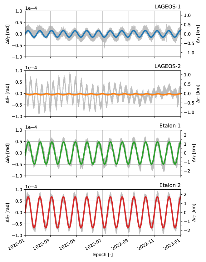
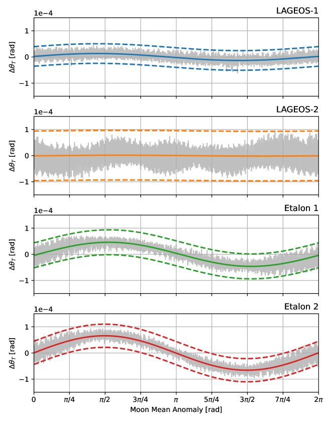
The fitted parameters for each of the calibration satellites, estimated using non-linear batch least squares, are presented in Table 4 and the corresponding models illustrated in Fig. 3. The Etalon 1 and 2 satellites showed good agreement with the model, with their respective parameters; however, LAGEOS-1 showed slightly different behaviour with an additional longer term variation, while LAGEOS-2 showed a complete lack of agreement with the simplified model caused by the presence of error oscillations at higher frequency.

Table 4: Fitted parameters for the bias model, expressing time in days since midnight on the 1^st January 2022.

Satellite	$a$ [rad]	$b$ [days]	$c$ [days]	$d$ [rad]
LAGEOS-1	$1.41\text{\times}{10}^{-5}$	$27.5$	$6.82\text{\times}{10}^{-2}$	$-1.79\text{\times}{10}^{-8}$
LAGEOS-2	$2.28\text{\times}{10}^{-6}$	$26.6$	$-1.19\text{\times}{10}^{1}$	$-4.00\text{\times}{10}^{-6}$
Etalon 1	$4.82\text{\times}{10}^{-5}$	$27.5$	$-9.17\text{\times}{10}^{-1}$	$-4.43\text{\times}{10}^{-7}$
Etalon 2	$6.75\text{\times}{10}^{-5}$	$27.6$	$-1.80\text{\times}{10}^{-1}$	$7.79\text{\times}{10}^{-8}$

The period of the along-track error model had significant agreement between LAGEOS-1 and Etalon 1 and 2 at approximately 27.5 days. This is very close to the Moon’s sidereal orbital period (approximately 27.3 days), supporting the suggestion that mismodelling of the Moon’s third-body perturbation in SGP4 is a contributing factor to the along-track error. The mismodelling error may result from either, or a combination of, the lunar ephemerides used by SGP4 or a lack of modelling of lunar long-periodic terms. The phase offsets also showed good agreement, varying by less than one day between the satellites, suggesting that it may be possible to constrain these parameters to constants across all of the satellites.

Fig. 3: Along-track errors of TLE with respect to SLR. The SLR data and fitted models are presented in grey and colour respectively.

Pseudo-observations are debiased by subtracting the modelled biases from the observation vector:

$$\mathbf{y}_{\text{debiased}}=\mathbf{y}-\mathbf{y}_{\text{bias}}\text{,}$$ (29)

resulting in an updated version of Eq. 14 which considers the effect of the bias:

$$\mathbf{b}_{\text{debiased}} =\mathbf{y}_{\text{debiased}}-\mathbf{y}^{*}\text{,}$$ (30)

$$=\mathbf{y}-\mathbf{y}_{\text{bias}}-\mathbf{y}^{*}\text{,}$$ (31)

where $\mathbf{b}_{\text{debiased}}$ is the debiased residual vector.

3 Bias Impact on P-OD Prediction Accuracy

3.1 Calibration Satellite Fits

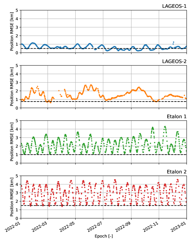
The quality of the calibration satellites’ TLE was evaluated fits to provide a benchmark for fit performance. The position RMSE for the TLE of the calibration satellites are presented in Fig. 4, calculated by propagating each of the TLE for 30 days after their epoch and evaluating their RMSE with respect to the SLR-derived states. All four calibration satellites showed periodic variations in RMSE throughout the year, albeit with differing behaviours. LAGEOS-1 had largely periodic behaviour which remained below $1\text{\,}\mathrm{km}$ for the majority of the year. Etalon 1 and 2 had higher RMSE with larger oscillations which remained bounded between approximately $1\text{\,}\mathrm{km}4.5\text{\,}\mathrm{km}$ and $1.5\text{\,}\mathrm{km}4.5\text{\,}\mathrm{km}$ respectively. Notably, the frequency of the error behaviour for Etalon 1 and 2 was approximately double that of LAGEOS-1. LAGEOS-2 had the most irregular behaviour with no obvious pattern, remaining bounded between approximately $0.75\text{\,}\mathrm{km}2.5\text{\,}\mathrm{km}$. The lower bounds of these errors provided a useful point of reference: consistently meeting the bound throughout the year alone would be a significant improvement as this would lead to the removal of the oscillations and more consistent state estimates.

Fig. 4: Position RMSE, with respect to SLR, during 30 days post-epoch for calibration satellite TLE. The dashed lines represent the established baselines for each satellite.

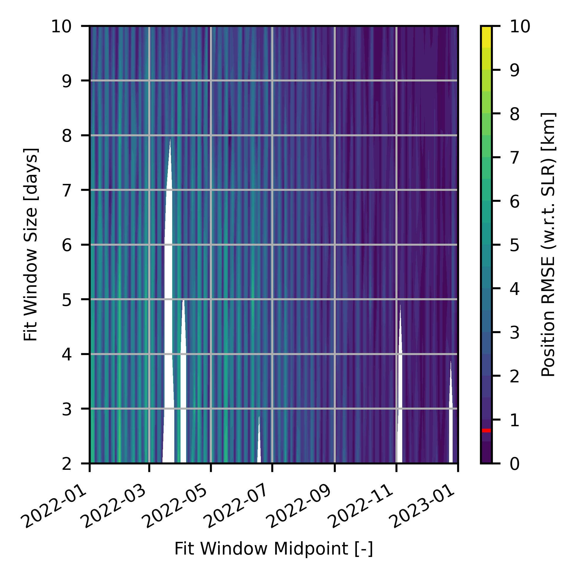
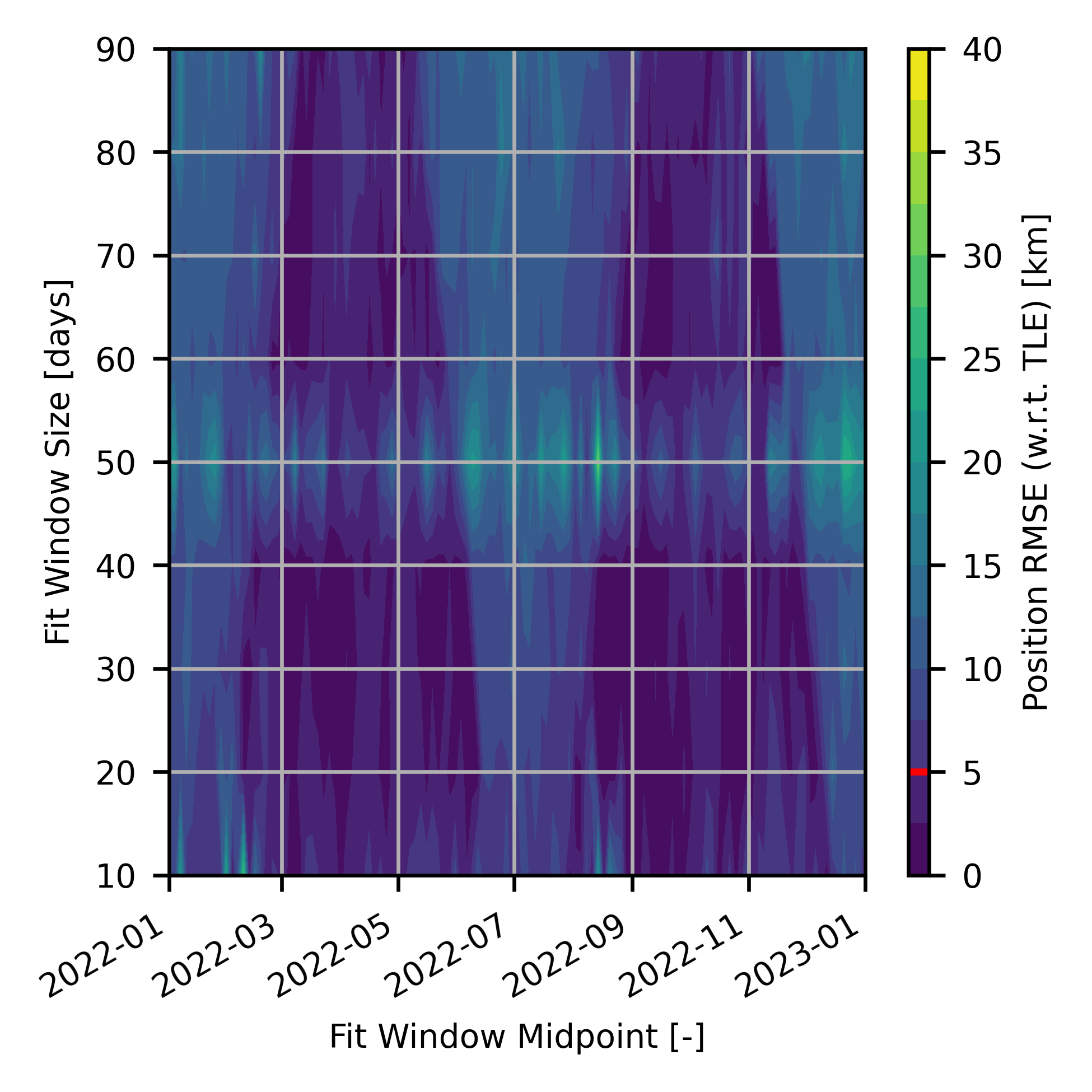
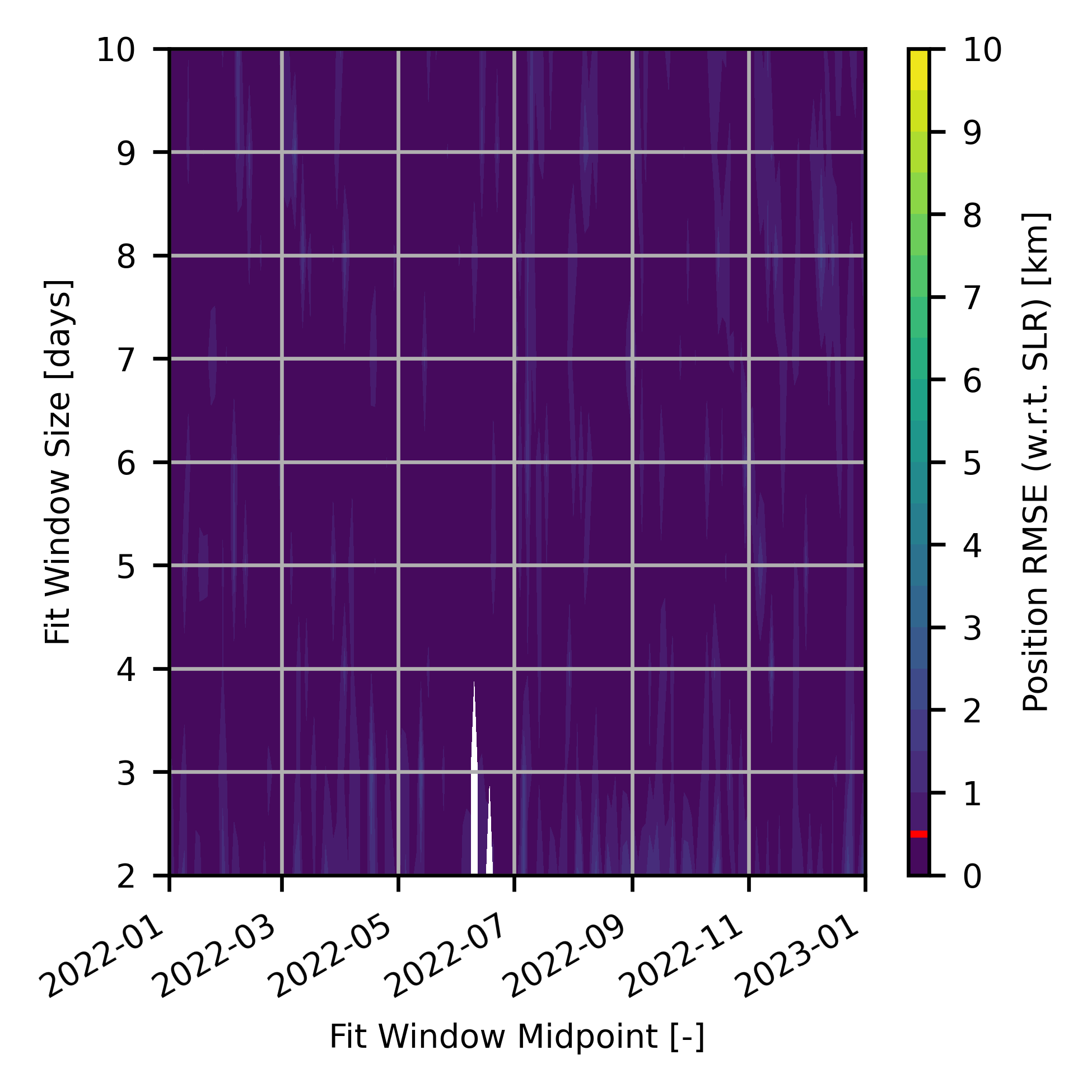
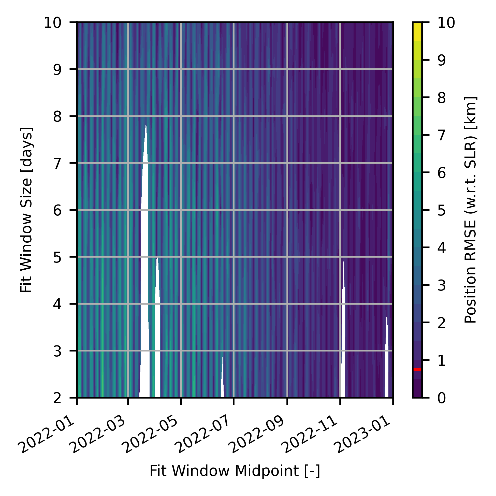
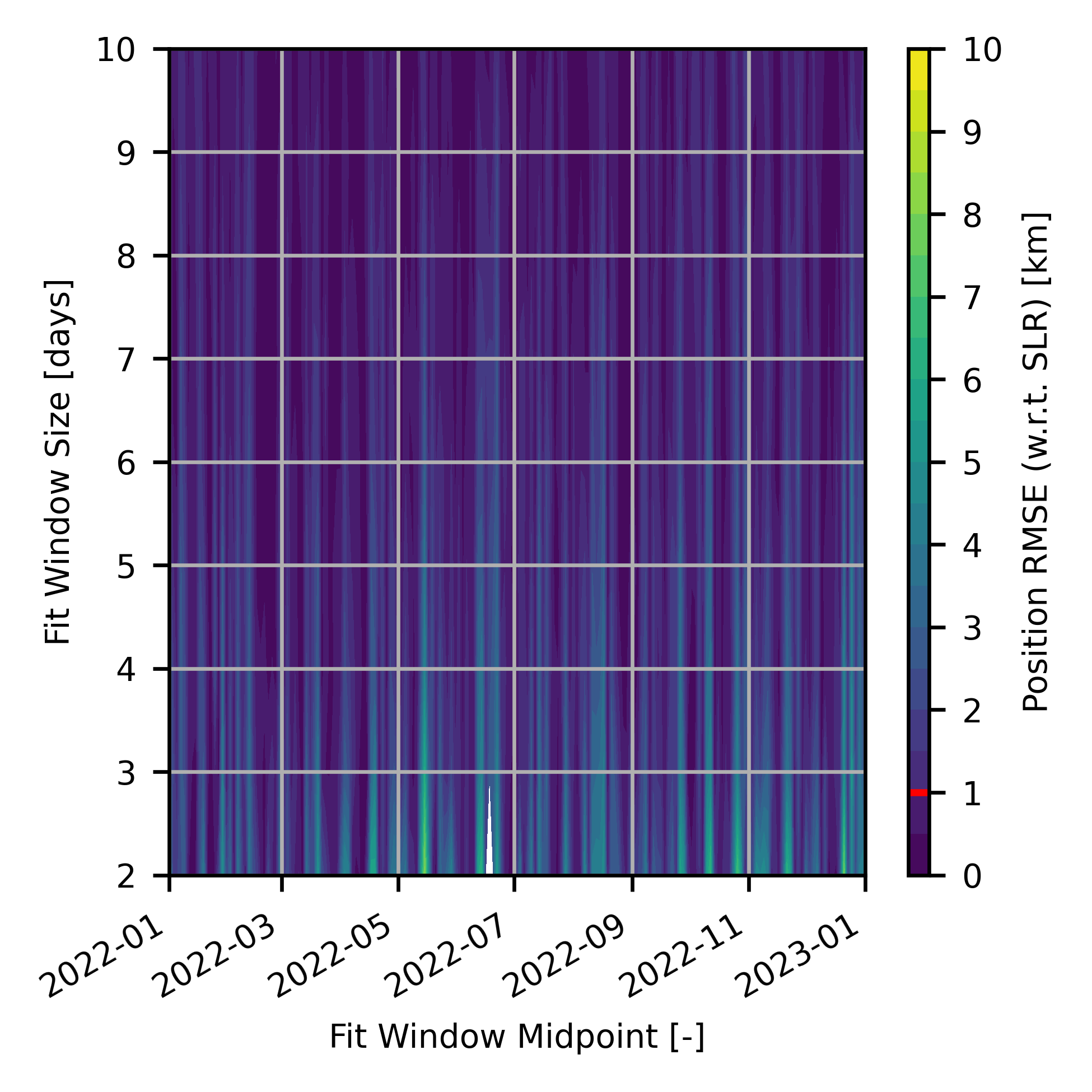
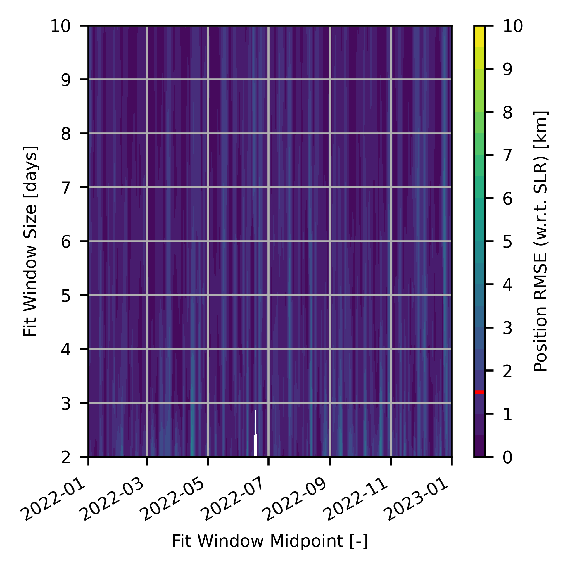
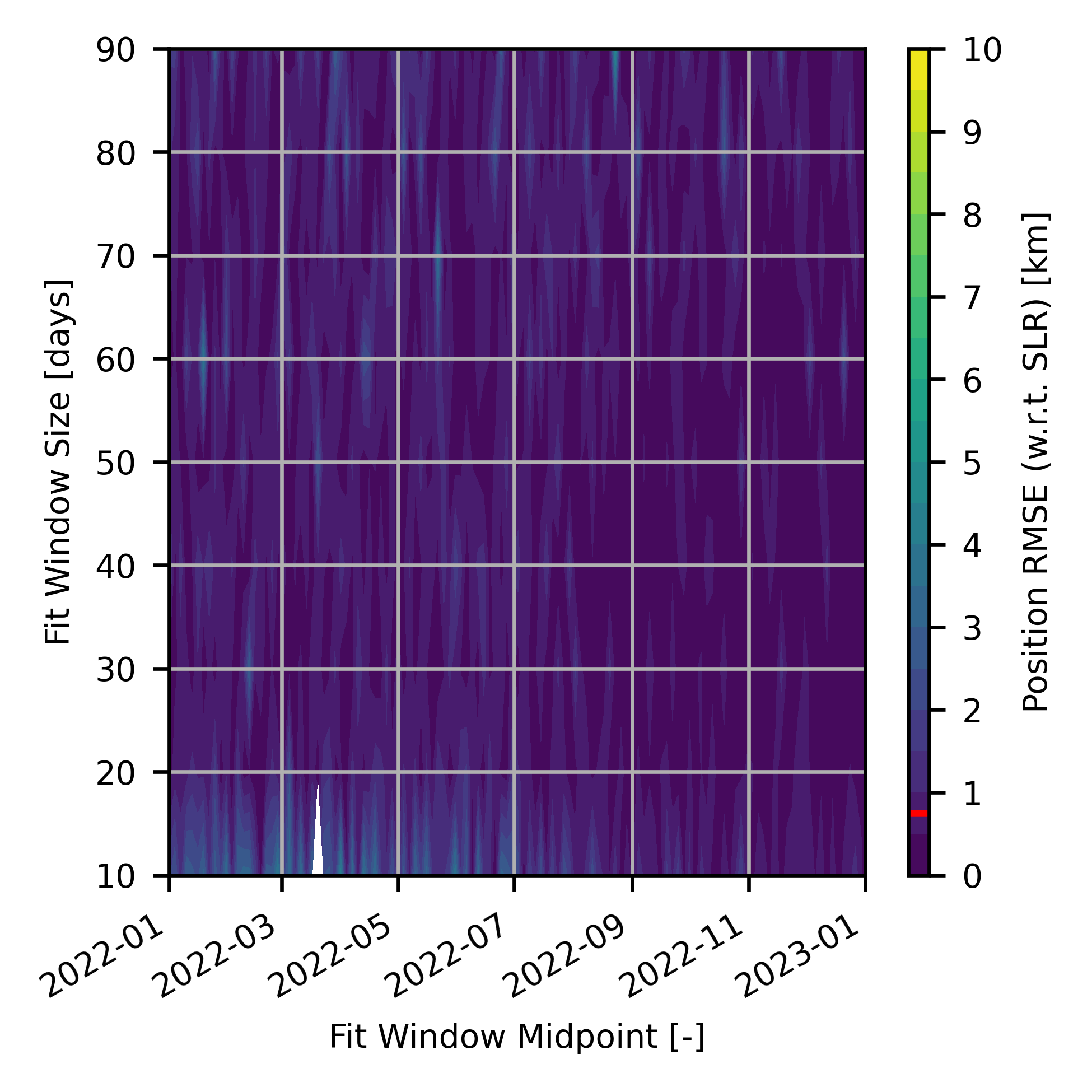
Fits on the calibration satellites were conducted using TLE and SLR data from the year 2022, considering combinations of fit midpoints and window sizes, as presented in Table 5. The motivation of these tests was to investigate the influence of the fit epoch and fit window size on the quality of fits, and whether a specific combination of these parameters was particular effective in mitigating the impact of biases in pseudo-observations. The results of conducting these fits are presented in Figs. 5 and 6.

Table 5: Fit sweep parameters.

Term	Fit midpoint period [days]	Number of samples [-]	Fit window size [days]
Short	2	100	2, 3, 4, 5, 6, 7, 8, 9, 10
Long	3	100	10, 20, 30, 40, 50, 60, 70, 80, 90

(a) LAGEOS-1.

(b) LAGEOS-2.

(c) Etalon 1.

(d) Etalon 2.

Fig. 5: Position RMSE during the 30 days post-fit for short-term biased fits. The red marker in the colour bar indicates the RMSE baseline derived from TLE. Note that white regions indicate failed cases due to an insufficient number of TLE.

(a) LAGEOS-1.

(b) LAGEOS-2.

(c) Etalon 1.

(d) Etalon 2.

Fig. 6: Position RMSE during the 30 days post-fit for long-term biased fits. The red marker in the colour bar indicates the RMSE baseline derived from TLE. Note that white regions indicate failed cases due to an insufficient number of TLE.

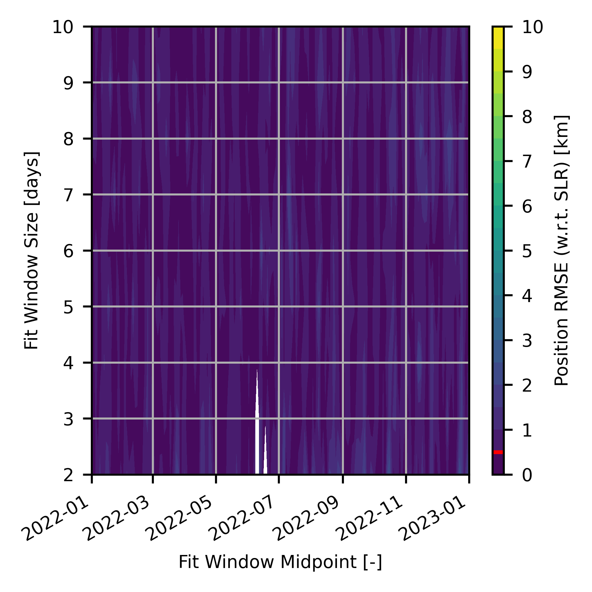
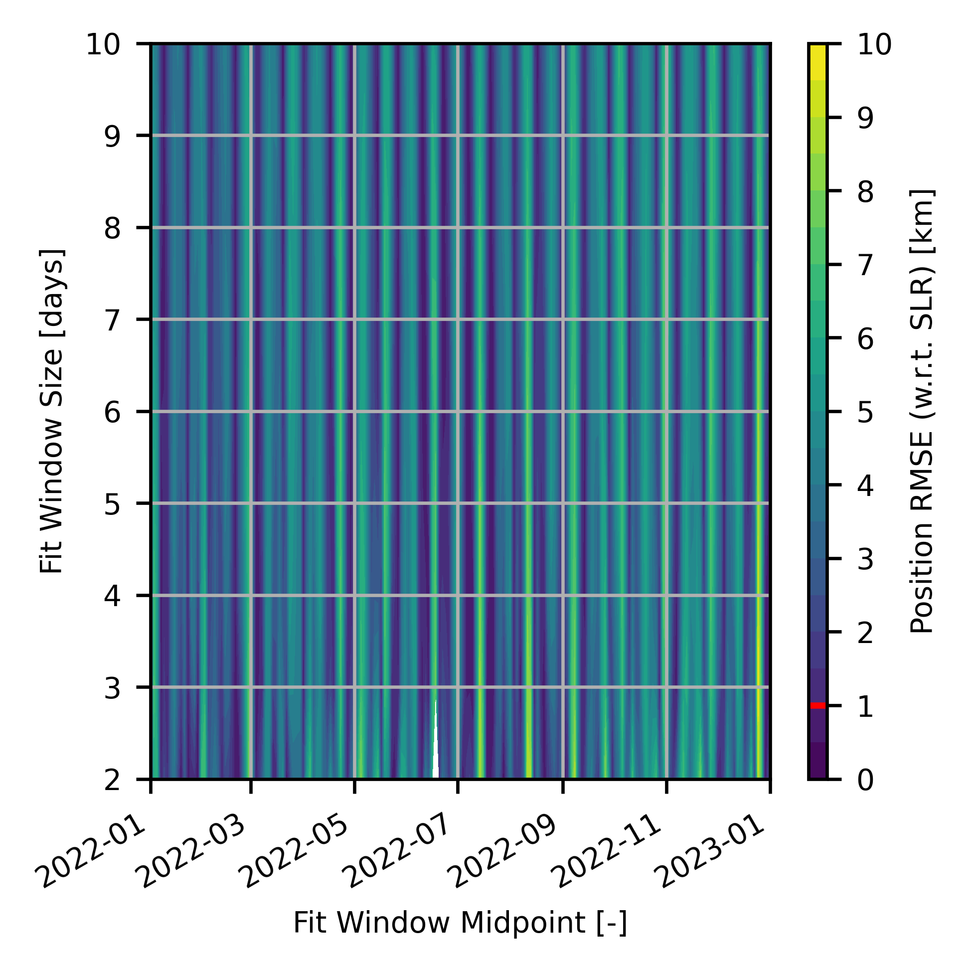
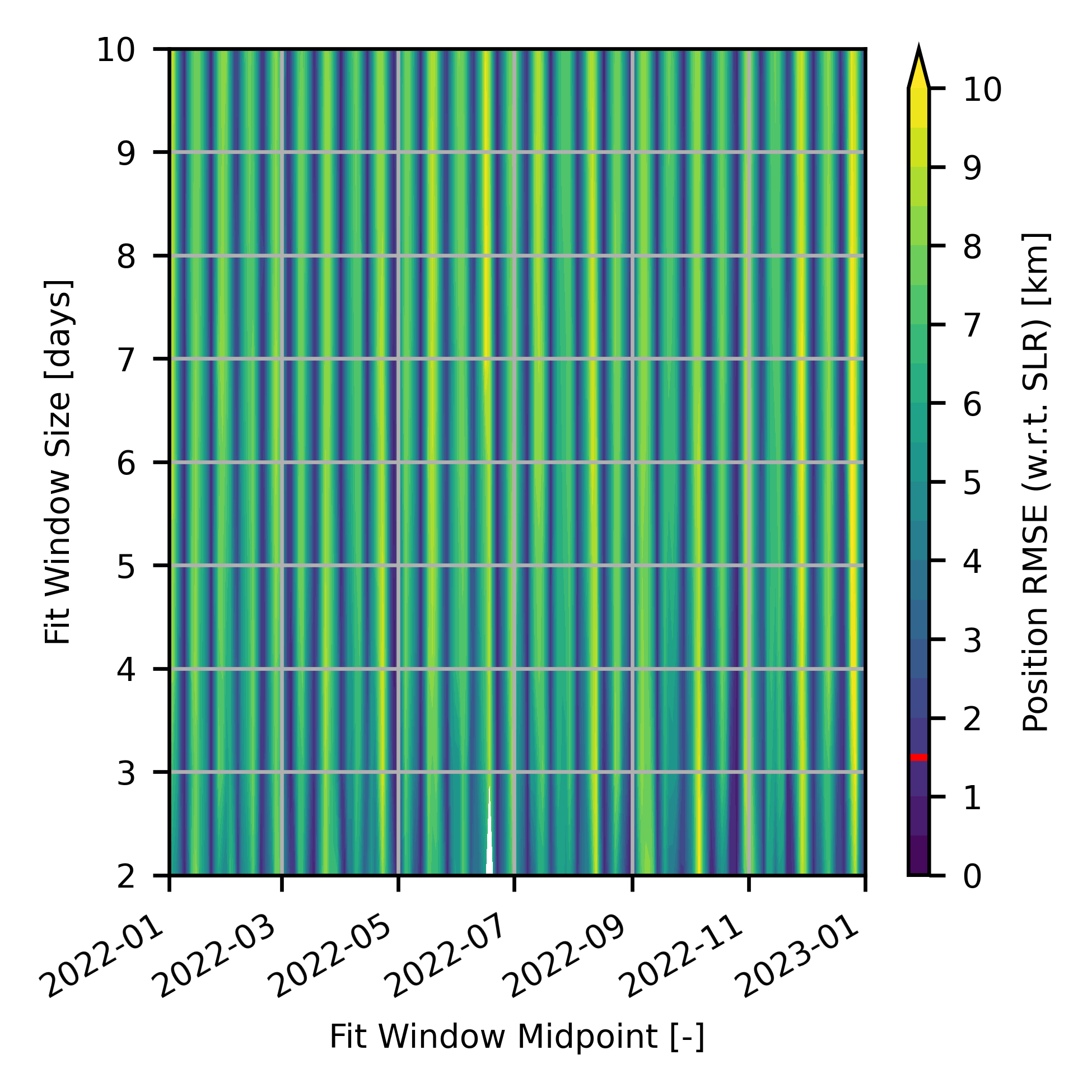
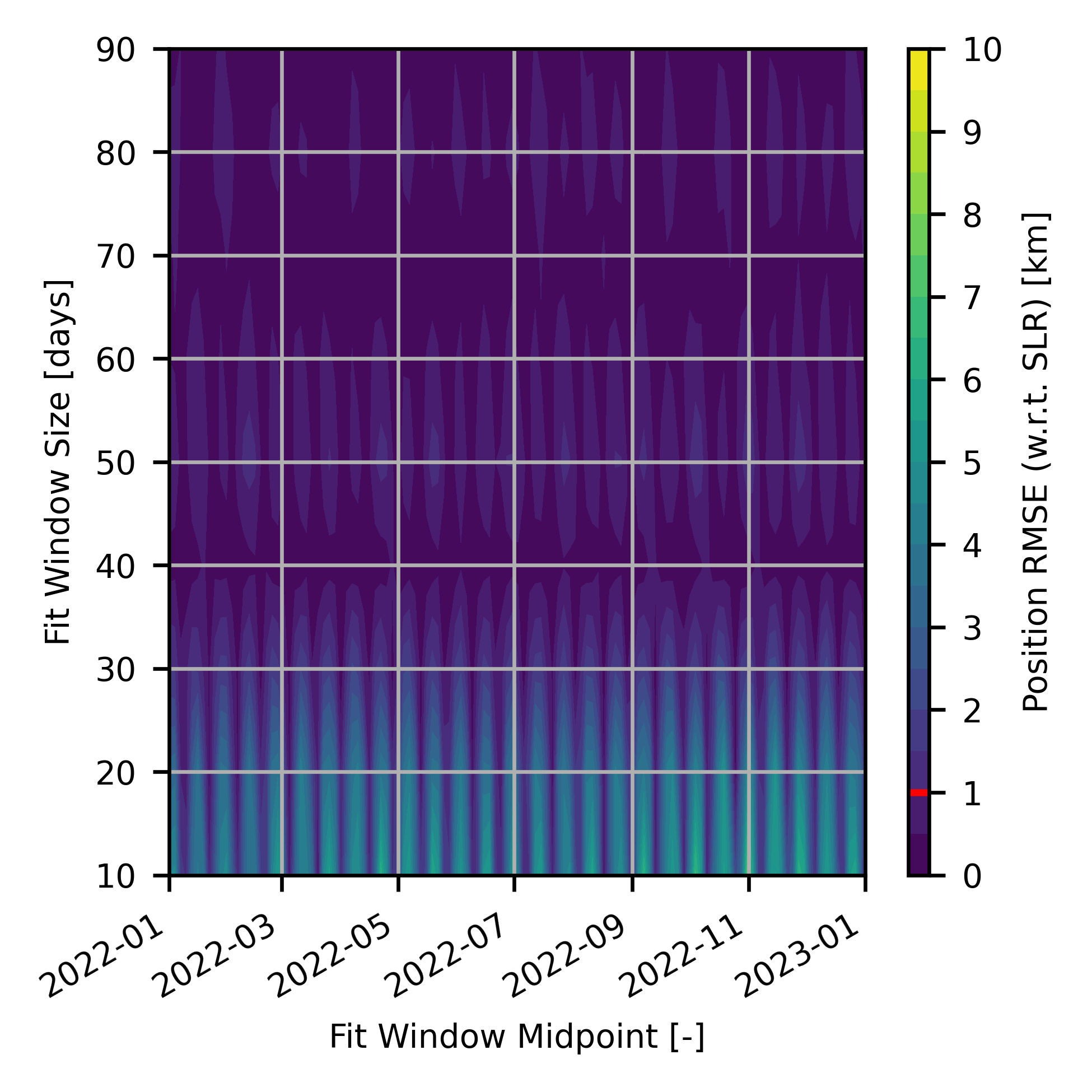
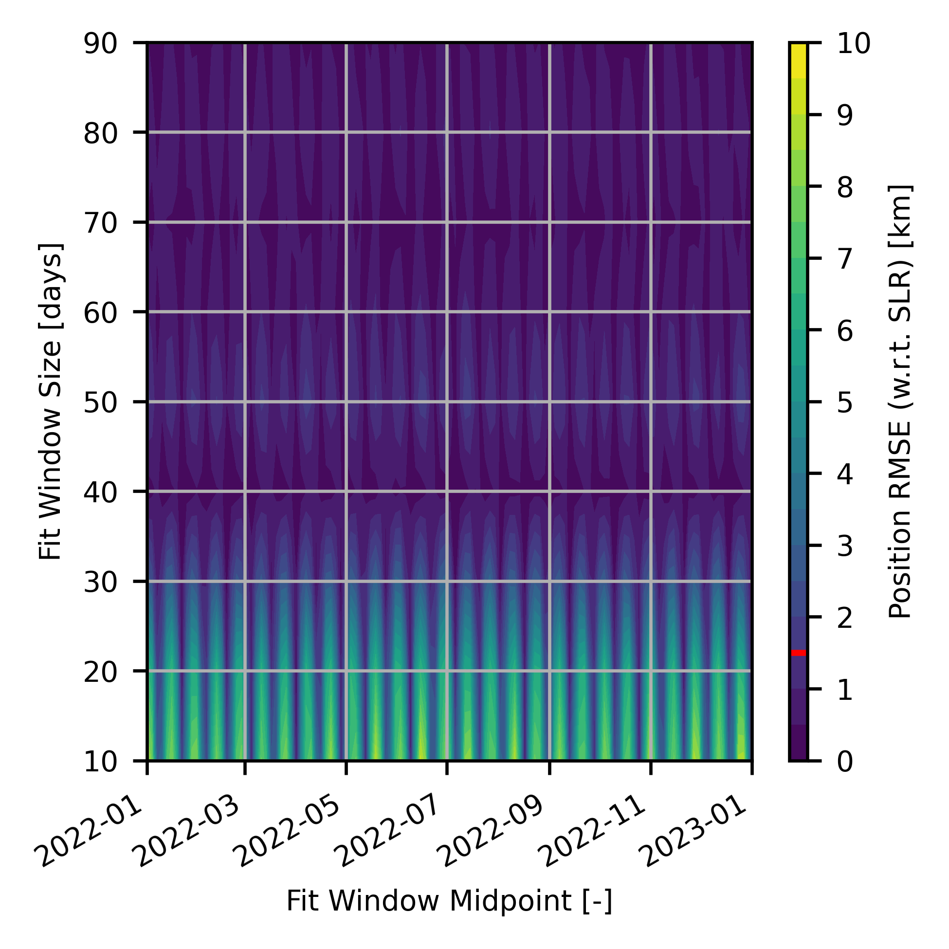
Fits on all four of the calibration satellites showed similar behaviour for the short-term cases: fit error was primarily driven by the fit window midpoint, noticeable as vertical banding throughout the year, particularly for Etalon 1 and 2. Fit window size appeared to have minimal impact on the fit error for the short-term cases with increased sizes not being associated with any change in error. LAGEOS-2 saw a significant improvement in fit quality towards the end of 2022, both in terms of typical error and the magnitude of the oscillations. This was associated with the reduction in along-track bias magnitude, as seen in Fig. 3.

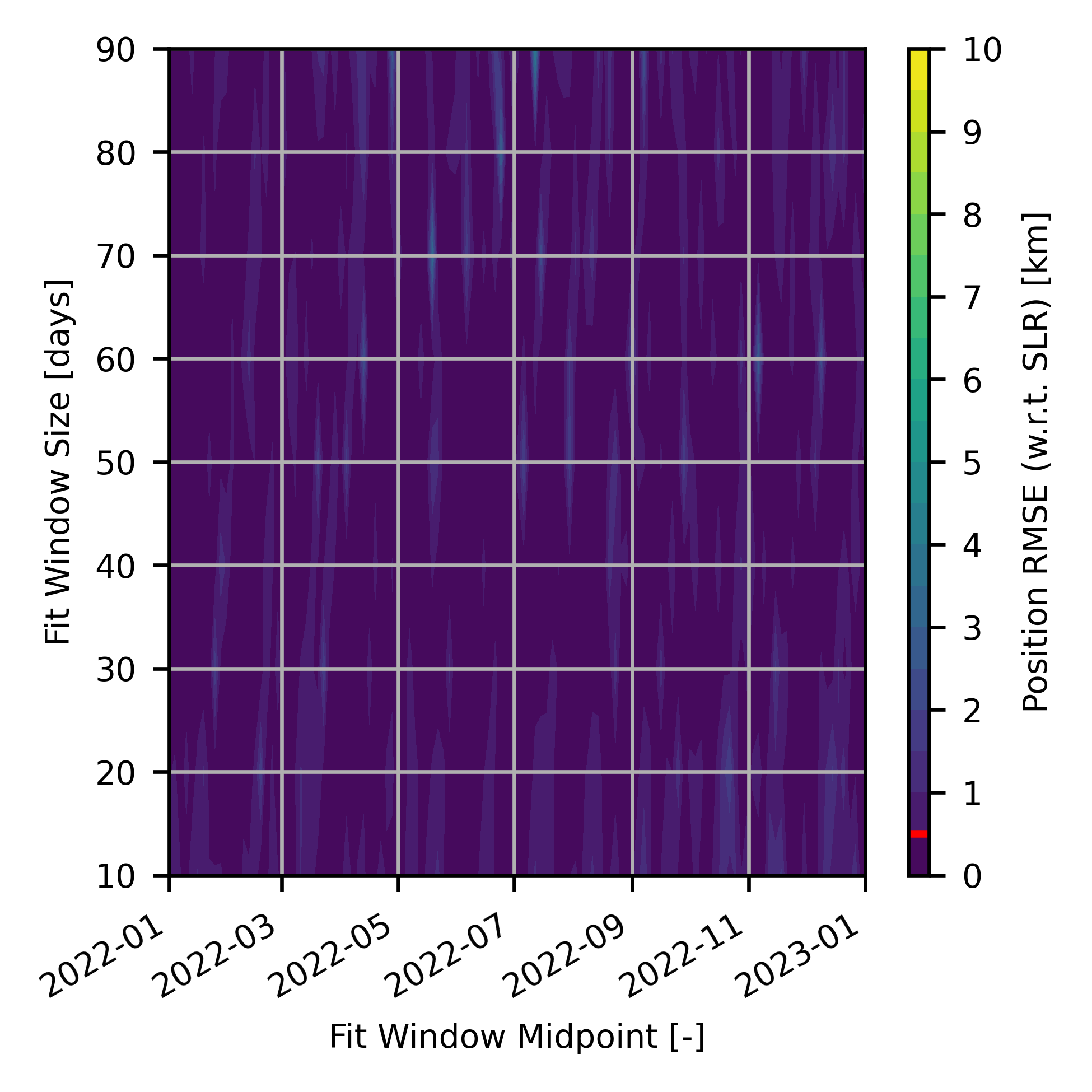
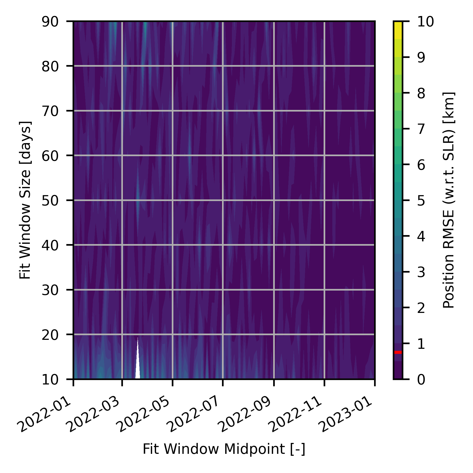
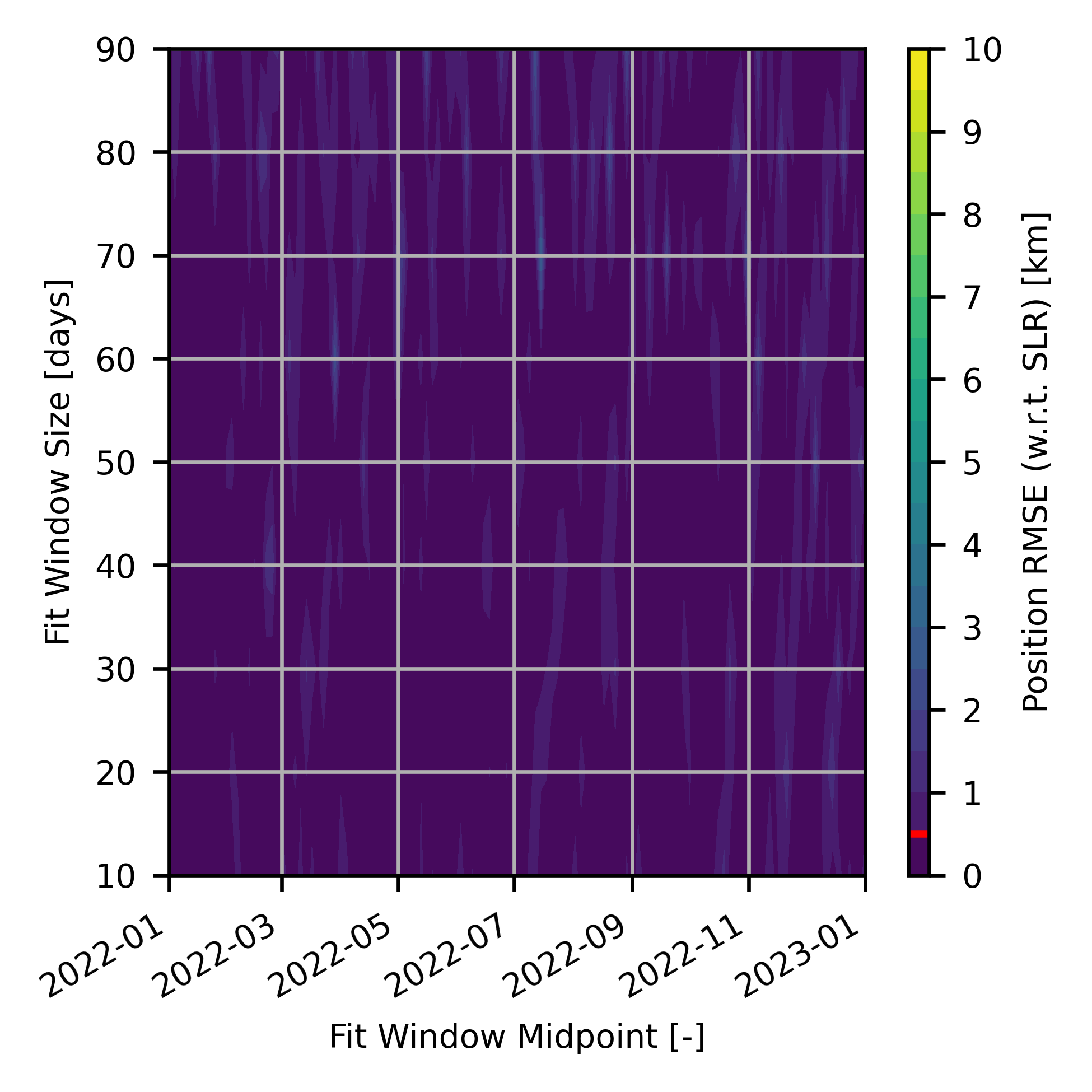
For the long-term fits, the dependence on fit midpoint remained for smaller windows. Nevertheless, the variation throughout the year reduced as the size of the windows increased. Above 40 days, the oscillations in fit error became significantly smaller for all four satellites, eventually converging to errors significantly lower than those seen for the short-term fits. Notably, for Etalon 1 and 2, some slight banding reappeared for fit windows around 50 days and 80 days, which demonstrated that the periodic influence of the bias was not completely eliminated in all cases by extending the fit windows. In any case, for the extended windows, the post-fit errors were typically at or below the baselines established in Fig. 4, suggesting that, for long-term fits, prediction accuracy was improved over the best case TLE-based predictions.

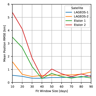
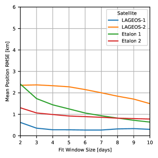
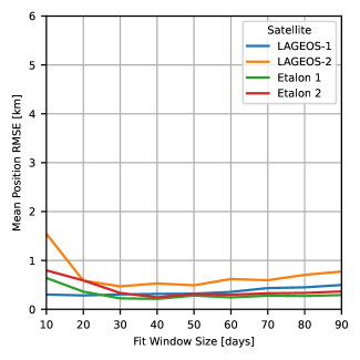
The impact of increasing the size of the fit window was further illustrated by considering the aggregate behaviour on fit error for each object. The mean position RMSE for each object as a function of the fit window size is presented in Fig. 7. For the short-term fits, the mean error remained largely constant for all four objects, other than a slight reduction for LAGEOS-2 and slight increase for Etalon 2. Significant reductions did not occur until the fit window size was increased past 10 days with all four objects reaching their respective baselines after 40 days. The slight banding for Etalon 1 and 2 at 50 days and 80 days was seen as slight increases in the mean error.

(a) Short-term.

(b) Long-term.

Fig. 7: Mean position RMSE during the 30 days post-fit for biased fits.

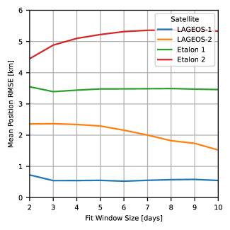
Importantly, many of the short-term fits had significantly higher errors than simply propagating TLE directly with SGP4. For example, fits on Etalon 1 and 2 often had errors double that of the worst cases presented in Fig. 4. This indicated that P-OD cannot be applied without careful selection of parameters nor without considering the impact of bias. In the absence of bias modelling, long fit windows are required to successfully apply P-OD techniques to TLE series.

3.2 Error Metric Correlation

The TLE-based error metric for estimating fit quality in the absence of SLR data captures errors resulting from both the fit and from the bias and noise in the TLE themselves. It was expected, therefore, that a lower bound would exist for this metric, representing the error of the TLE alone for a hypothetical perfect fit with no error with respect to the true state of the satellite. Nonetheless, for a poor fit which diverges significantly from the true state of the satellite, the errors resulting from the fit become more significant than the intrinsic TLE errors, therefore the two metrics should see greater alignment. These expected behaviours are illustrated in Fig. 8.

(a) TLE dominated, where the errors in the TLE themselves drive the error.

(b) Fit dominated, where the errors in the fit drive the error.

Fig. 8: Illustration of error metric scenarios.

A comparison of the SLR- and TLE-based position RMSE is presented in Fig. 9. The TLE-based errors were generally larger than SLR-based errors. The TLE-based metric had a highly apparent lower bound for each of the four objects, matching the expected behaviour. For larger errors, a more linear behaviour was seen between the metrics.

Fig. 9: Comparison between SLR- and TLE-based position RMSE during the 30 days post-fit with linear regressions for each satellite. The dashed line indicates equal RMSE.

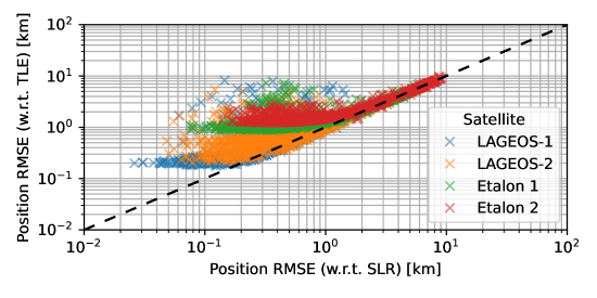
The results of conducting linear regression on the error metrics, above a minimum error cut-off and in the more linear region, are presented in Table 6. Apart from LAGEOS-1, the Pearson correlation coefficients ($\rho$) were near unity indicating very strong correlation. Furthermore, the slopes would suggest a near 1:1 relationship between the metrics.

Table 6: Results of linear regression between the SLR- and TLE-based metrics for SLR-based errors above $1\text{\,}\mathrm{km}$.

Satellite	Slope [-]	Intercept [km]	$\rho$ [-]
LAGEOS-1	0.81	0.53	0.43
LAGEOS-2	0.98	0.12	0.98
Etalon 1	0.91	0.40	0.98
Etalon 2	0.92	0.51	0.99

Importantly, the very strong correlation in error metrics suggested that the TLE-based metric could be used, at the very minimum, for relative comparisons of fit quality for a single object. This result meant that it was feasible to use the TLE-based metric for fit quality evaluation of any object in the TLE catalogue, allowing testing to be extended to any object meeting the non-manoeuvring requirement.

3.3 Test Satellite Fits

The lack of “ground truth” data for the test satellites, from either SLR or pseudo-ranging, meant that the TLE-based error metric had to be used to compare fit quality. This was based on the analysis presented in Section 3.2 demonstrating the strong correlation between SLR- and TLE-based error metrics. Additionally, to smooth out the effect of the variations in TLE quality on the reference solution, the prediction duration was extended to 90 days.

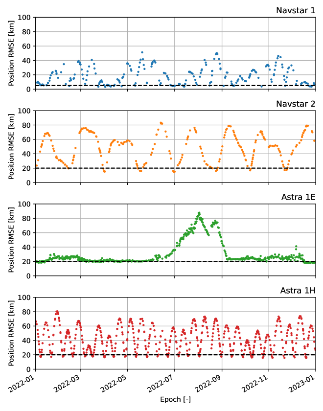
The quality of the test satellites’ TLE, relative to future TLE, was evaluated to establish a benchmark for each satellite, as in Section 3.1. The results are presented in Fig. 10. Navstar 1 and 2, and Astra 1H showed periodic behaviour in error throughout the year, although seemingly each with different structures and periods. In the case of Navstar 1, the errors remained below $50\text{\,}\mathrm{km}$ throughout the year. In the case of Navstar 2 and Astra 1H, the errors oscillated in a band from $20\text{\,}\mathrm{km}80\text{\,}\mathrm{km}$. Astra 1E had errors which remained around $20\text{\,}\mathrm{km}$ consistently with little variation, apart from a period between July and September where the error grew significantly to $90\text{\,}\mathrm{km}$.

Fig. 10: Position RMSE, with respect to TLE, during 90 days post-epoch for test satellite TLE. The dashed lines represent the established baselines for each satellite.

The results of fits on the test satellites are presented in Fig. 11. In general, fits on the four objects showed large domains where the fit performance meets or exceeds the benchmark, suggesting that the fits were successfully reducing the prediction errors with respect to propagating the TLE directly. Increasing the fit window size was generally beneficial, although the error behaviour was more complex than for test objects and fits were highly dependent on the quality of the TLE within and following the fit window.

(a) Navstar 1.

(b) Navstar 2.

(c) Astra 1E.

(d) Astra 1H.

Fig. 11: Position RMSE during the 90 days post-fit for long-term biased fits. The red marker in the colour bar indicates the RMSE baseline derived from TLE.

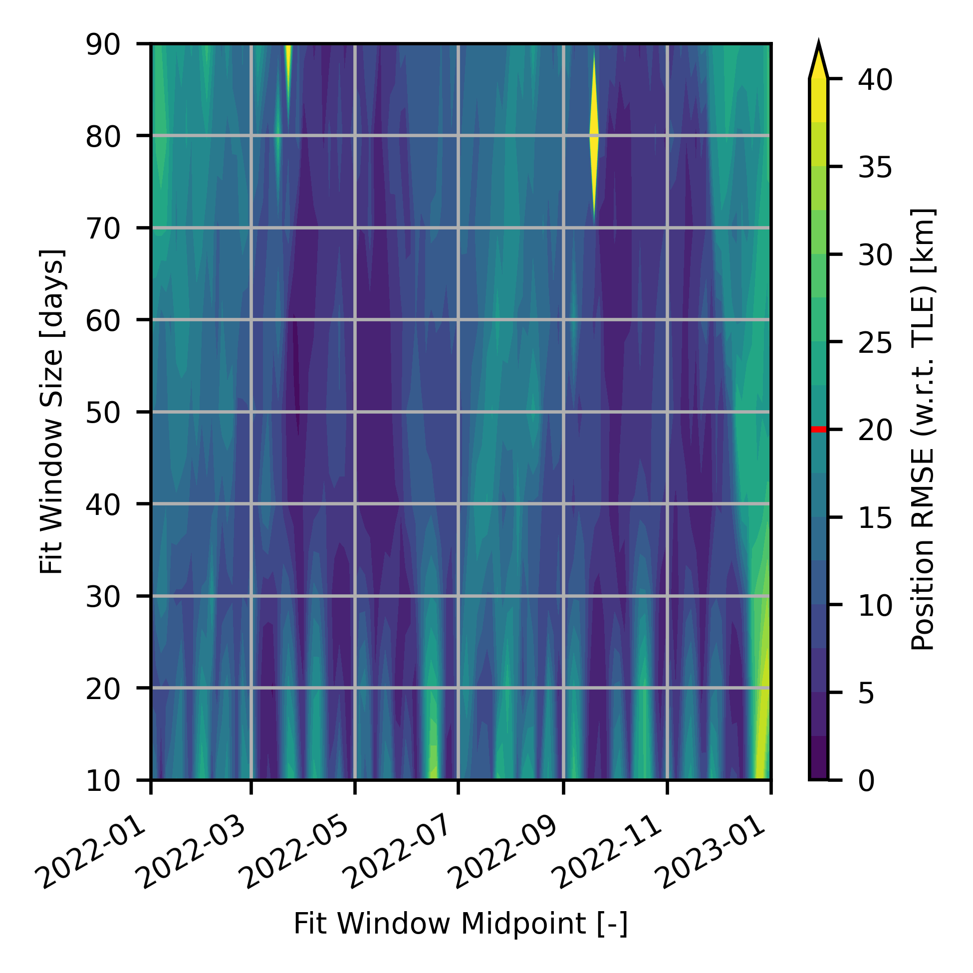
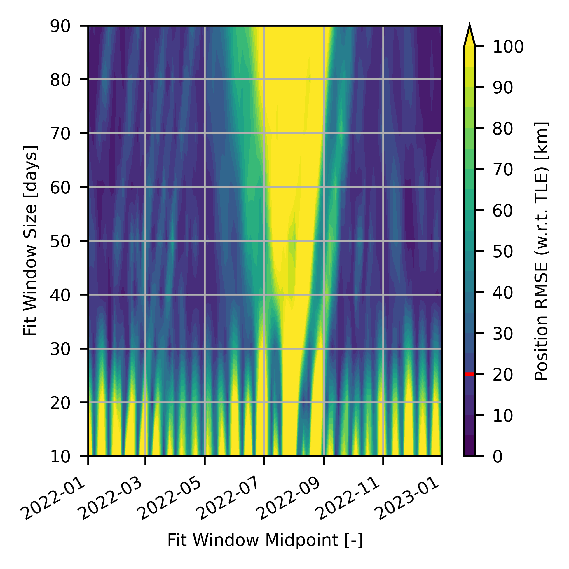
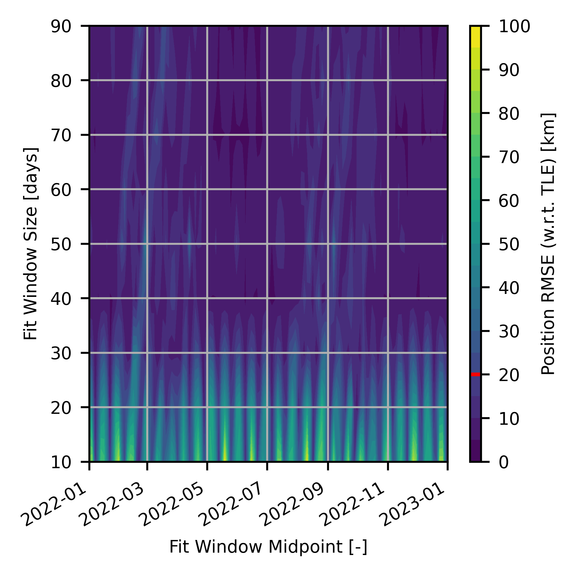
The periodic variation in error throughout the year for short fit windows was highly apparent for Navstar 2, and Astra 1E and 1H. The fits on Navstar 1, on the other hand, did not show this variation as strongly, instead demonstrating a longer period variation throughout the year with slightly increased errors at two points in the year, November through February and June through August. Nevertheless, along with Astra 1H, a notable increase in periodic error was visible for 50-day windows, a duration close to twice the Moon’s orbital period. The increased TLE error for Astra 1E between July and September was highly apparent, as seen by very high errors for the fits during the time period. It was unexpected that Navstar 1 would not show oscillatory behaviour in the fits despite oscillations in TLE quality, and vice versa for Astra 1E, which showed oscillatory behaviour for short-term windows despite constant TLE-on-TLE error.

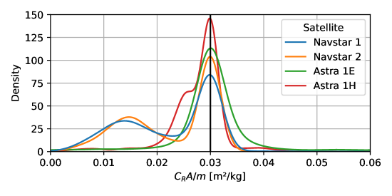
The distributions of the estimated SRP coefficients are presented in Fig. 12. For all four objects, the majority of fits resulted in coefficients close to the initial guess of $3\text{\times}{10}^{-2}\text{\,}\mathrm{m}^{2}\mathrm{/}\mathrm{k}\mathrm{g}$. It was expected that the majority of estimated SRP coefficients would remain in the region of the initial guess due to the aforementioned low observability of the parameter during the P-OD process. In the case of Navstar 1 and 2, a second peak was visible around $1.5\text{\times}{10}^{-2}\text{\,}\mathrm{m}^{2}\mathrm{/}\mathrm{k}\mathrm{g}$.

Fig. 12: SRP coefficient distributions for the test satellites fits.

4 Debiased P-OD

4.1 Calibration Satellite Fits

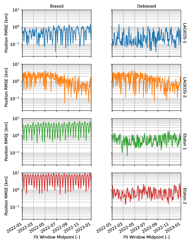
The results of fits on the test satellites, following debiasing as described in Section 2.7, are presented in Figs. 13 and 14. The fits on LAGEOS-1 saw minor reductions in error with some suppression of the periodic behaviour for short fit windows. The results for LAGEOS-2 remained mainly unaffected, demonstrating the same error behaviour as the fits on the biased pseudo-observations. This was expected due to the corresponding debiasing model have very little impact on the along-track position. The fits on Etalon 1 and 2 saw the most significant changes in error: although the periodic variations were still visible, the peak errors were reduced from approximately $10\text{\,}\mathrm{km}$ to $2\text{\,}\mathrm{km}$.

(a) LAGEOS-1.

(b) LAGEOS-2.

(c) Etalon 1.

(d) Etalon 2.

Fig. 13: Position RMSE during the 30 days post-fit for short-term debiased fits. The red marker in the colour bar indicates the RMSE baseline derived from TLE. Note that white regions indicate failed cases due to an insufficient number of TLE.

(a) LAGEOS-1.

(b) LAGEOS-2.

(c) Etalon 1.

(d) Etalon 2.

Fig. 14: Position RMSE during the 30 days post-fit for long-term debiased fits. The red marker in the colour bar indicates the RMSE baseline derived from TLE. Note that white regions indicate failed cases due to an insufficient number of TLE.

The suppression of the oscillations in error was seen in the reduction of the mean position RMSE in Fig. 15. For short-term fits of Etalon 1, the mean position error was reduced from an approximately constant $3.5\text{\,}\mathrm{km}$ to a trend decreased from approximately $2.5\text{\,}\mathrm{km}0.5\text{\,}\mathrm{km}$, representing an approximate $30\text{\,}\%85\text{\,}\%$ reduction in error. For Etalon 2, the mean error was reduced from approximately $5\text{\,}\mathrm{km}$ to $1\text{\,}\mathrm{km}$, an $80\text{\,}\%$ reduction. For the long-term fits, in addition to the mean position errors converging sooner for a small fit window size, the peaks at 50 and 80 days were removed with mean errors remaining below $1\text{\,}\mathrm{km}$ after fit windows larger than 20 days.

(a) Short-term.

(b) Long-term.

Fig. 15: Mean position RMSE during the 30 days post-fit for debiased fits.

4.2 Effect of Fit Window on Bias Impact

The influence of window size on the bias can be analysed by considering the mean bias during the window. For the simplified sinusoidal model, Eq. 28, this can be found through direct, analytical integration:

$$\overline{\Delta\theta_{T}}(t^{*},\Delta t) =\frac{1}{\Delta t}\int_{t^{*}-\frac{\Delta t}{2}}^{t^{*}+\frac{\Delta t}{2}}\Delta\theta_{T}(t)\ dt\text{,}$$ (32)

$$\approx\frac{1}{\Delta t}\int_{t^{*}-\frac{\Delta t}{2}}^{t^{*}+\frac{\Delta t}{2}}a\sin\left(\frac{2\pi}{b}\left(t+c\right)\right)+d\ dt\text{,}$$ (33)

$$\approx\frac{ab}{\pi\Delta t}\sin\left(\frac{2\pi}{b}\left(t^{*}+c\right)\right)\sin\left(\frac{\pi\Delta t}{b}\right)+d\text{,}$$ (34)

where $\overline{\Delta\theta_{T}}$ is the mean along-track angular error, $t^{*}$ is the mid-point of the window, and $\Delta t$ its size.

The same method can be used to find the mean bias error rate during the window:

$$\overline{\Delta\dot{\theta}_{T}}(t^{*},\Delta t) =\frac{1}{\Delta t}\int_{t^{*}-\frac{\Delta t}{2}}^{t^{*}+\frac{\Delta t}{2}}\Delta\dot{\theta}_{T}(t)\ dt\text{,}$$ (35)

$$=\frac{1}{\Delta t}\left[\vphantom{\frac{1}{1}}\Delta\theta_{T}(t)\right]_{t^{*}-\frac{\Delta t}{2}}^{t^{*}+\frac{\Delta t}{2}}\text{,}$$ (36)

$$\approx\frac{1}{\Delta t}\left[a\sin\left(\frac{2\pi}{b}\left(t+c\right)\right)+d\right]_{t^{*}-\frac{\Delta t}{2}}^{t^{*}+\frac{\Delta t}{2}}\text{,}$$ (37)

$$\approx\frac{2a}{\Delta t}\cos\left(\frac{2\pi}{b}\left(t^{*}+c\right)\right)\sin\left(\frac{\pi\Delta t}{b}\right)\text{,}$$ (38)

where $\overline{\Delta\dot{\theta}_{T}}$ is the mean along-track angular error rate.

A key feature of the mean error is that the period and phase remain unchanged by the averaging process, remaining independent of the fit window size. This would explain why the variations in position RMSE showed the same pattern as the fit window size was increased. The mean error rate, on the other hand, is phase-shifted by $90\text{\,}\mathrm{d}\mathrm{e}\mathrm{g}$ with respect to the mean error. Putting aside the influence of the sine term for one moment, this would suggest that the amplitude of the mean error rate is highest when the mean error is minimised and vice-versa, as illustrated in Fig. 16.

(a) Centred about a zero crossing, demonstrating zero mean error but a non-zero mean error rate.

(b) Centred about a peak, demonstrating a non-zero mean error but zero mean error rate.

Fig. 16: Example of averaging a bias model (blue), illustrated by considering a line of best fit (red) for a restricted domain (black, dashed).

Increasing the size of the fit window has important effects on the mean error and mean error rate. The amplitude of the periodic terms are reduced due to the inclusion of the reciprocal of the fit window size as a coefficient. In the limit, this results in the periodic behaviour being removed entirely:

$$\lim_{\Delta t\to\infty}\overline{\Delta\theta_{T}}(t^{*},\Delta t) \approx d\text{,}$$ (39)

$$\lim_{\Delta t\to\infty}\overline{\Delta\dot{\theta}_{T}}(t^{*},\Delta t) \approx 0\text{.}$$ (40)

Alternatively, the mean error and error rate can be minimised by considering the sinusoidal component present in both Eqs. 34 and 38:

$$\sin\left(\frac{\pi\Delta t}{b}\right) =0\text{,}$$ (41)

$$\frac{\pi\Delta t}{b} =\pi n\text{,}$$ (42)

$$\frac{\Delta t}{b} =n\text{,}$$ (43)

where $n$ is an integer. In other words, the mean along-track angular error and error rate are minimised when the fit window duration is an integer multiple of the bias period. It is worth noting that this does not match the behaviour seen in the test satellite fits, where the position RMSE appeared to increase rather than decrease near the integer multiples. A potential cause of this discrepancy might include the additional harmonics seen in the TLE data, or the need for a more accurate bias model.

The effect of extending the fit window is to convert short-term biases into long-term noise. By capturing multiple cycles of the bias, with a period of approximately 27.5 days as identified in Section 2.7, the mean along-track error averages to near-zero. This is due to times of the TLE leading and lagging the true position cancelling out. This results in a solution to the batch least squares process which is not strongly influenced by the bias in a small part of the cycle.

4.3 Alternative Bias Models

The main limitation of the along-track error model was that it was not generalised for any satellite, a shortcoming present in many of the models proposed in previous literature. Fundamentally, this is a result of creating models based on a small subset of objects with known precise ephemerides which may not represent the wider catalogue.

In the case of the model presented above, amplitudes varied by satellite, and LAGEOS-1 showed slightly different behaviour to the Etalon satellites. The outlying behaviour of LAGEOS-2 raises the question of whether other satellites will have similar behaviour, and whether it is a direct result of the SGP4 model, the dynamics of specific orbital regimes, or additional non-physical factors introduced during the TLE generation process. Additional components of the state vector may benefit also from debiasing: although not implemented here, the radial velocity was found to have similar periodic variations with respect to epoch.

The key for future bias model development lies with the careful selection of which parameters are included as inputs. These can dramatically affect both the model’s performance and whether it is generalisable to a larger proportion of the TLE catalogue. For example, the lunar perturbation is a product of the distance between the satellite and the Moon, therefore it may be appropriate to include the Moon’s position as a parameter in a bias model. In the case of Eq. 28, the use of time could be seen as a proxy for the Moon’s position, supported by the fitted models’ period closely matching that of the Moon.

An alternative bias model, based on the Moon’s position along its orbit is presented:

$$\Delta\theta_{T}(M)\approx a\sin(M+b)\text{,}$$ (44)

where $M$ is the Moon’s mean anomaly, and $a$ and $b$ are the bias amplitude and phase offset respectively.

While this model adds some complexity over Eq. 28, due to requiring ephemerides for the Moon, it is still relatively simple computationally. Furthermore, it is linked more directly to the suspected source of the bias, mismodelling of the lunar perturbation, than indirectly via time.

The fitted parameters for the anomaly-based bias model are presented in Table 7. As expected, the amplitudes of the model are very similar to those presented in Table 4, including the very small value for LAGEOS-2, suggesting a similarly poor fit. Notably, the phase offsets for LAGEOS-1, and Etalon 1 and 2 are very similar, lying within a $0.26\text{\,}\mathrm{r}\mathrm{a}\mathrm{d}$ band.

Table 7: Fitted parameters for the anomaly-based bias model.

Satellite	$a$ [rad]	$b$ [rad]
LAGEOS-1	$1.33\text{\times}{10}^{-5}$	$1.73\text{\times}{10}^{-1}$
LAGEOS-2	$1.82\text{\times}{10}^{-6}$	$-3.23\text{\times}{10}^{-1}$
Etalon 1	$4.62\text{\times}{10}^{-5}$	$-8.40\text{\times}{10}^{-2}$
Etalon 2	$6.59\text{\times}{10}^{-5}$	$9.97\text{\times}{10}^{-3}$

The anomaly-based bias models are illustrated in Fig. 17. The model for LAGEOS-2 can be seen to match poorly with the variations in the along-track bias, appearing similar to a horizontal line through zero. The variations in along-track bias for LAGEOS-2 appear to have higher frequency components, suggesting that higher frequency terms should be considered. For LAGEOS-1, and Etalon 1 and 2 the models show good agreement visually with all variations lying within the $3\sigma$ bounds. In the case of Etalon 1 and 2, the amplitude of the noise about the model appears to increase in the region near perilune. This would be logical given the increased magnitude of the perturbation as the Moon makes its closest approach to Earth and the satellites.

Fig. 17: Along-track bias model, based on the Moon’s mean anomaly. The SLR data and fitted models are presented in grey and colour respectively, with the dashed lines representing the $3\sigma$ bounds.

Data-driven solutions, such as the simplified models presented in this study or other machine learning methods (Ly et al., 2020), are limited to the availability of “ground truth” data, such as from SLR or post-processed pseudoranging, for training, validation, and testing. Furthermore, for objects with high quality “ground truth” data, it is unknown whether these higher accuracy products are used during the TLE generation process and whether this means that these satellites have TLE sets with differing characteristics. The question remains, therefore, whether bias models developed using these objects can be extrapolated to other satellites and objects in the TLE catalogue.

On the other hand, an alternative source of “ground truth” data, or more accurately, approximate “ground truth” data, might be derived from the TLE themselves using P-OD. By conducting long-term fits, as demonstrated in Section 3.3, the approximate true trajectory of a given object can be extracted and then compared to the underlying TLE to estimate their bias. This method remains restricted to passive objects due to the non-manoeuvring requirement, however due to the large number of passive objects in the TLE catalogue, such as decommissioned satellites, rocket bodies, and other debris, it should be possible to generate a large dataset for this analysis.

4.4 Fit Covariance Analysis

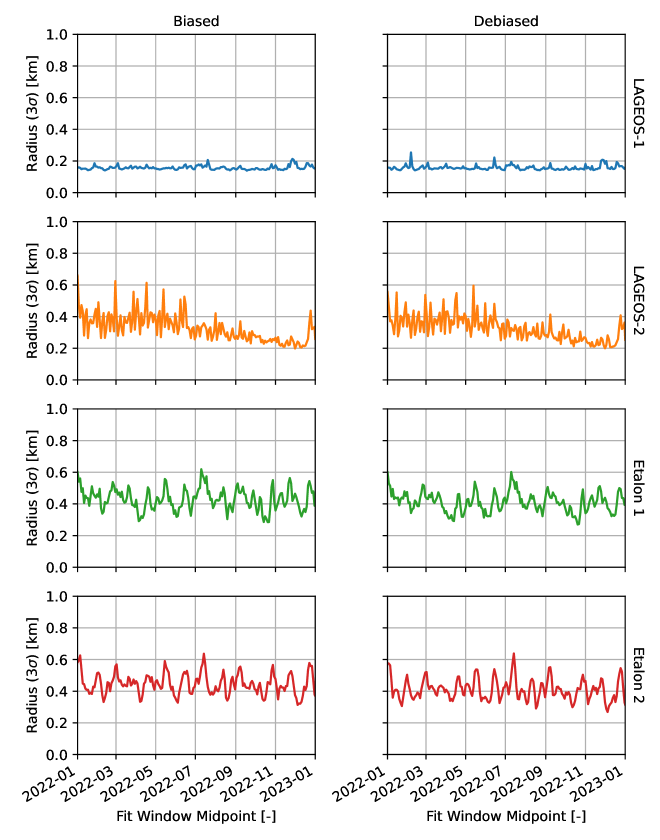
A comparison of short-term fits conducted on the four calibration satellites, both without and with debiasing with the simplified model, are presented in Fig. 18. For the satellites with the best-fitting bias models, Etalon 1 and 2, debiasing had a significant impact on post-fit position RMSE, as described in Section 4.1. The equivalent radii of the position residual covariances for the four calibration satellites are presented in Fig. 19. In contrast to the position RMSE, the equivalent radii throughout the year for all four objects appeared largely unaffected by the debiasing of the pseudo-observations. This suggested that the covariance alone was a poor indicator for the quality of the fit.

Fig. 18: Position RMSE during the 30 days post-fit for the LAGEOS and Etalon satellites as a function of fit window midpoint for 10-day fits.

Fig. 19: Equivalent radius of the position residuals for the LAGEOS and Etalon satellites as a function of fit window start for 10-day fits.

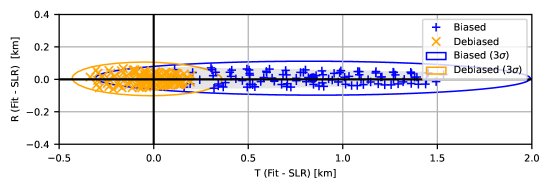
Examples of the residual scatter, the differences between the predicted and observed states at each observation time in the fit window, relative both to the TLE-based pseudo-observations and the SLR-based “ground truth”, for short- and long-term fits are presented in Figs. 20 and 21. The fit residuals for the short-term window, as presented in Fig. 20(a), remained largely unaffected in aggregate by the debiasing process. Although individual points shifted, in some cases by up to $0.5\text{\,}\mathrm{km}$ in the tangential direction, the overall distribution, and hence covariance, remained approximately the same. When considering the residuals with respect to the “ground truth” in Fig. 20(b), however, a large change was visible with the both the mean of the distribution shifting towards the origin and the covariance shrinking in the tangential axis. This relationship was reversed for the case of the long-term fit window: debiasing resulted in a significant reduction in the variance along the tangential axis for the fit residuals, while the residuals with respect to the “ground truth” appeared less affected in aggregate.

(a) With respect to TLE.

(b) With respect to SLR.

Fig. 20: Example residual scatters in the radial-transverse plane for a short-term Etalon 1 fit.

(a) With respect to TLE.

(b) With respect to SLR.

Fig. 21: Example residual scatters in the radial-transverse plane for a long-term Etalon 1 fit.

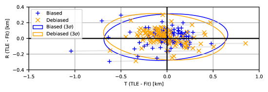
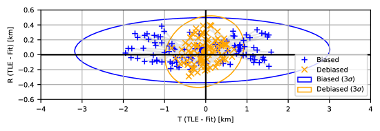
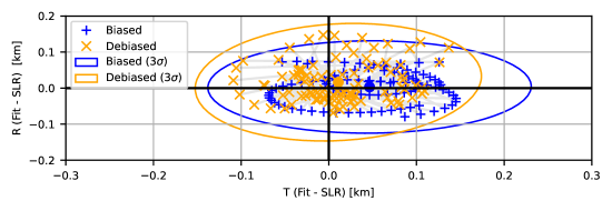
The systematic variation in along-track error means that the biases in successive TLE are highly correlated. The period of this variation is much longer than the short-term fit window sizes, therefore the pseudo-observations have similar, correlated biases. In effect, the biased TLE are representing physically accurate and consistent orbits, however not matching the true orbits of the satellites on short time scales. The debiasing process reduces the mean error of the pseudo-observations with respect to the true state, however the noise remains unaffected. This highlights that the covariance cannot be used as an indicator for fit accuracy as it is unaffected by the biases.

5 Conclusions

Systematic along-track biases throughout the year were identified as the primary limiting factor in the quality of P-OD fits in the MEO regime. Mitigation of these biases was demonstrated to be key for improving the quality of higher precision ephemerides derived from TLE. Two strategies were proposed and demonstrated: extension of the fit windows to convert short-term biases into long-term noise, and a simple sinusoidal model for estimating along-track error. Both methods were effective at reducing the typical post-fit accuracy by approaching an order of magnitude for the selected calibration satellites, and suppressing oscillations in errors for the test satellites.

It has been shown that the covariance output from the P-OD process cannot be used to evaluate the prediction accuracy of a given fit. Many state estimation algorithms require that observations are unbiased and satisfy a given distribution, typically Gaussian, about the true states of a satellite. This requirement is not satisfied by uncorrected TLE-based pseudo-observations during short-term fit windows, resulting in fits which appear well correlated with pseudo-observations but, in reality, are poorly correlated with the true underlying state.

The TLE catalogue remains one of the few sources of ephemerides for a significant proportion of RSO in near-Earth orbits. Until Type 4 TLE are released publicly for a critical share of the catalogue, a combination of debiasing and P-OD will be required for deriving higher-precision ephemerides for many RSO. The development of generalised bias estimation models, covering multiple orbital regimes, will be crucial for improving P-OD applied to the TLE catalogue.

The analysis in this study was limited to only six passive satellites in MEO and two in GEO/GSO and, therefore, may not represent general TLE behaviour at these altitudes. There are additional calibration satellites available in this orbital regime with precision ephemerides which could be used for further investigation, namely the active satellites within various GNSS constellations. The satellites in these constellations have similar orbits to the Etalon and tested Navstar satellites, primarily in terms of semi-major axis, eccentricity, and inclination. Nevertheless, these satellites regularly manoeuvre for station-keeping which will need to be taken into account by any analysis of their TLE.

It is expected that TLE behaviour will be different in LEO due to the changes in perturbations model, notably the removal of lunisolar perturbations and SRP, but the inclusion of atmospheric drag. A separate investigation into the biases present in this orbital regime will be required. It is expected that the same systematic biases seen with MEO calibration satellites will not be present, instead replaced by issues with drag estimation, and sampling strategy as investigated by Chen & Lin (2023).

Several of the limitations of batch least squares methods can be addressed by sequential filters; therefore, these are the logical next step for improving TLE-based P-OD. These types of filters lend themselves naturally to solution updates as new TLE are published by USSF, and allow for physical parameters to be included in the estimation process continuously, such as ballistic coefficient for LEO. The state of the art solution for sequential P-OD is to use an UKF, initialised with an initial state and covariance from a batch least squares solution. Nevertheless, it should be noted that both batch least squares methods and sequential filters will be susceptible to biases in the pseudo-observations without the ability to detect degraded estimates through the covariance. TLE biases must be addressed before conducting any P-OD, particularly with methods which only consider the pseudo-observed states over a short time period.

References

- Amato et al. (2018) Amato, D., Rosengren, A. J., & Bombardelli, C. (2018). THALASSA: a fast orbit propagator for near-Earth and cislunar space. In 2018 Space Flight Mechanics Meeting AIAA SciTech Forum. Kissimmee, FL, USA: American Institute of Aeronautics and Astronautics.
- Araya & Amato (2022) Araya, I. A., & Amato, D. (2022). Spectral analysis of US Space Catalog ephemerides for LAGEOS-1. In AIAA SCITECH 2022 Forum. San Diego, CA, USA: American Institute of Aeronautics and Astronautics.
- Baù et al. (2014) Baù, G., Urrutxua, H., & Pelaez, J. (2014). EDROMO: An accurate propagator for elliptical orbits in the perturbed two-body problem. Adv. Astronaut. Sci., 152, 379–399.
- Bennett et al. (2012) Bennett, J. C., Sang, J., Smith, C. et al. (2012). Improving low-Earth orbit predictions using two-line element data with bias correction. In Advanced Maui Optical and Space Surveillance Technologies Conference. Maui, HI, USA.
- Biancale et al. (2000) Biancale, R., Balmino, G., Lemoine, J.-M. et al. (2000). A new global Earth’s gravity field model from satellite orbit perturbations: GRIM5-S1. Geophysical Research Letters, 27(22), 3611–3614.
- Chao & Hoots (2018) Chao, C.-C., & Hoots, F. R. (2018). Applied Orbit Perturbation and Maintenance. (2nd ed.). El Segundo, CA, USA: The Aerospace Press.
- Chen & Lin (2023) Chen, J., & Lin, C. (2023). Research on Enhanced Orbit Prediction Techniques Utilizing Multiple Sets of Two-Line Element. Aerospace, 10(6).
- Conkey & Zielinski (2022) Conkey, D., & Zielinski, M. (2022). Assessing Performance Characteristics of the SGP4-XP Propagation Algorithm. In Advanced Maui Optical and Space Surveillance Technologies Conference. Maui, HI, USA.
- ESA (2023) ESA (2023). ESA’s Annual Space Environment Report. LOG GEN-DB-LOG-00288-OPS-SD ESA Space Debris Office Darmstadt, Germany. URL: https://www.sdo.esoc.esa.int/environment_report/Space_Environment_Report_latest.pdf.
- Folkner et al. (2014) Folkner, W. M., Williams, J. G., Boggs, D. H. et al. (2014). The Planetary and Lunar Ephemerides DE430 and DE431, .
- Geul et al. (2017) Geul, J., Mooij, E., & Noomen, R. (2017). TLE uncertainty estimation using robust weighted differencing. Advances in Space Research, 59(10), 2522–2535.
- Hallgarten La Casta & Amato (2024) Hallgarten La Casta, M. I., & Amato, D. (2024). Revisiting Filtering of Two-line Element Sets for Higher Precision Ephemerides. In 29th International Symposium on Space Flight Dynamics. Darmstadt, Germany.
- Hejduk et al. (2013) Hejduk, M. D., Casali, S. J., Cappellucci, D. A. et al. (2013). A catalogue-wide implementation of general perturbations orbit determination extrapolated from higher order orbital theory solutions. In AAS/AIAA Spaceflight Mechanics Meeting. Kauai, HI, USA. AAS 13-240.
- Hindmarsh (1982) Hindmarsh, A. C. (1982). ODEPACK, A Systematized Collection of ODE Solvers. URL: https://computing.llnl.gov/sites/default/files/ODEPACK_pub1_u88007.pdf.
- Holincheck & Cathell (2021) Holincheck, A., & Cathell, J. (2021). Improved Orbital Predictions using Pseudo Observations - Maximizing the Utility of SGP4-XP. In Advanced Maui Optical and Space Surveillance Technologies Conference. Maui, HI, USA.
- Hoots et al. (2004) Hoots, F. R., Schumacher, P. W., & Glover, R. A. (2004). History of Analytical Orbit Modeling in the US Space Surveillance System. Journal of Guidance, Control, and Dynamics, 27(2), 174–185.
- Levenberg (1944) Levenberg, K. (1944). A Method for the Solution of Certain Non-Linear Problems in Least Squares. Quarterly of Applied Mathematics, 2(2), 164–168.
- Levit & Marshall (2011) Levit, C., & Marshall, W. (2011). Improved orbit predictions using two-line elements. Advances in Space Research, 47(7), 1107–1115.
- Ly et al. (2020) Ly, D., Lucken, R., & Giolito, D. (2020). Correcting TLEs at epoch: Application to the GPS constellation. Journal of Space Safety Engineering, 7(3), 302–306.
- Maisonobe et al. (2010) Maisonobe, L., Pommier, V., & Parraud, P. (2010). Orekit: an Open-source Library for Operational Flight Dynamics Applications. In 4th ICATT International Conference on Astrodynamics Tools and Techniques. Madrid, Spain.
- Marquardt (1963) Marquardt, D. W. (1963). An Algorithm for Least-Squares Estimation of Nonlinear Parameters. Journal of the Society for Industrial and Applied Mathematics, 11(2), 431–441.
- Payne et al. (2022) Payne, T., Hoots, F., Butkus, A. et al. (2022). Improvements to the SGP4 propagator (SGP4-XP). In Advanced Maui Optical and Space Surveillance Technologies Conference. Maui, HI, USA.
- Pearlman et al. (2019) Pearlman, M., Arnold, D., Davis, M. et al. (2019). Laser geodetic satellites: a high-accuracy scientific tool. Journal of Geodesy, 93(11), 2181–2194.
- Racelis & Joerger (2018) Racelis, D., & Joerger, M. (2018). High-Integrity TLE Error Models for MEO and GEO Satellites. In 2018 AIAA SPACE and Astronautics Forum and Exposition. Orlando, FL, USA.
- Tapley et al. (2004) Tapley, B. D., Schutz, B. E., & Born, G. H. (2004). Statistical orbit determination. Amsterdam, the Netherlands: Elsevier Academic Press.
- Vallado (2013) Vallado, D. A. (2013). Fundamentals of Astrodynamics and Applications. (4th ed.). Hawthorne, CA, USA: Microcosm Press.
- Vallado et al. (2013) Vallado, D. A., Bastida Virgili, B., & Flohrer, T. (2013). Improved SSA through orbit determination of Two-Line-Element sets. In 6th European Conference on Space Debris (p. 7). Darmstadt, Germany.