Alexander polynomials of symplectic curves and divisibility relations

Abstract.

We prove Libgober’s divisibility relations for Alexander polynomials of symplectic curves in the complex projective plane. Along the way, we give new proofs of the divisibility relations for complex algebraic curves with respect to a generic line at infinity.

1. Introduction

The study of fundamental groups of complements of plane complex curves (and, more generally, of complex projective hypersurfaces) has a very rich history, dating back at least to the work of Zariski and van Kampen  [zar1, zar2]. Their pencil section method allows to find a presentation of $\pi_{1}(\mathbb{CP}^{2}\setminus\mathcal{C})$ for a complex curve $\mathcal{C}$. In the early 80s, Moishezon [Mo] introduced the notion of braid monodromy to give a similar presentation of the fundamental group; see also Libgober [Lib1], Cohen and Suciu [Cohen] for further advances and for more references.

Distinguishing groups directly from a presentation is hard. Like in classical knot theory, one can use the Alexander polynomial as a proxy to study the fundamental group (see, for istance, [Rolfsen, Section 7.D] or [Lickorish, Chapter 11]). In the context of complex curves in $\mathbb{CP}^{2}$ (and, more generally, of projective hypersurfaces), the Alexander polynomial was introduced and studied by Libgober in [Libcyclic]. To define it, one needs to choose an auxiliary line $L$. We will denote it with $\Delta_{\mathcal{C},L}$, but we will often drop $L$ from the notation when it is understood. Libgober also discovered a beautiful relation, not at all apparent from the definition, between the Alexander polynomial of a curve, the local Alexander polynomials of the links of its singularities, and the Alexander polynomial of the link at infinity of $\mathcal{C}$ (with respect to $L$).

1.1. Main results

We will prove that Libgober’s divisibility relations hold also for symplectic curves. Here we adopt the terminology of [golla_starkston_2022]: a symplectic curve is a (possibly singular) 2-dimensional submanifold of $\mathbb{CP}^{2}$ that is $J$-holomorphic for some almost-complex structure $J$ compatible with the Fubini–Study metric $\omega_{\rm FS}$ on $\mathbb{CP}^{2}$. For instance, (reduced) complex curves are by definition symplectic, and so are smoothly embedded symplectic surfaces of $\mathbb{CP}^{2}$.

Theorem 1.1.

Let $\mathcal{C}\cup L$ be a symplectic curve. Call $K_{1},\dots,K_{\nu}$ the links of its singularities, and $K_{\infty}$ the link at infinity of $\mathcal{C}$ with respect to $L$. Then

• $\Delta_{\mathcal{C},L}\mid\Delta_{K_{\infty}}$;

• $\Delta_{\mathcal{C},L}\mid\hat{\Delta}_{K_{1}}\cdots\hat{\Delta}_{K_{\nu}}\cdot(1-t)^{b_{1}(\mathcal{C}\cup L)}$; if $\mathcal{C}$ is irreducibile, one can get rid of the factors $1-t$ on the right-hand side.

In particular, this recovers Libgober’s result for complex curves. We would like to stress that our proofs are not just an adaptation of Libgober’s proofs. In fact, we also give alternative proofs in the case of complex curves (at least under the assumption that $L$ is generic) that have a more low-dimensional flavour than the original arguments.

Here, $\hat{\Delta}_{K_{i}}$ is a suitably twisted version of the classical Alexander polynomial of $K_{i}$, which can equivalently be described as a specific evaluation of the multi-variable Alexander polynomial of $K_{i}$. Whenever $K_{i}$ is the link of a singularity that is not on the line at infinity $L$, $\hat{\Delta}_{K_{i}}$ is just the usual (one-variable) Alexander polynomial of $K_{i}$.

As a corollary, we get strong restrictions on the polynomials that can arise as Alexander polynomials of symplectic curves.

Corollary 1.2.

The Alexander polynomial of a symplectic curve in $\mathbb{CP}^{2}$ is either $0$ or a product of cyclotomic polynomials.

Remark 1.3.

For instance, $\Delta_{\mathcal{C},L}$ does not vanish, and hence is a product of cyclotomic polynomials, in the following cases:

• if $L$ is transverse to $\mathcal{C}$;

• if $\mathcal{C}$ is a line arrangement, except for case where $\mathcal{C}\cup L$ is a pencil;

• if $\mathcal{C}$ is irreducible.

1.2. History and perspectives

As mentioned above, the fundamental groups of complements of complex curves are in general not easy to compute. In some cases, we know a priori that the group is Abelian, and having a presentation clearly suffices to compute the fundamental group very explicitly. This is the case, for instance, of nodal curves, curves whose singularities are only double points: see Zariski [Zariski, Section 3], Fulton [fulton], Deligne [Deligne].

In [zar2], Zariski computed the fundamental groups of the complements of the now-called Zariski sextics: this computation shows that the fundamental group of the complement of a complex curve is not in general determined by the degree of the curve and the types of its singularities, but it also depends on the position of the singularities. This lead to the definition of Zariski pairs, pairs of curves with the same combinatorics (same degree, same singularities, same incidence relations between components) but with non-homeomorphic complements. For an excellent historical and mathematical account of Zariski pairs, we recommend the survey by Artal Bartolo, Cogolludo Agustín, and Tokunuga [ACT-survey].

Zariski’s examples are two irreducible sextics with six singular points, all of which are simple cusps (locally modelled on $\{y^{2}=x^{3}\}\subset\mathbb{C}^{2}$), and therefore of genus $4$. One of the two sextics, $\mathcal{C}_{1}$, has all of its singular points lying on a conic, and has fundamental group $\mathbb{Z}/2\mathbb{Z}*\mathbb{Z}/3\mathbb{Z}$, while the other one, $\mathcal{C}_{2}$, does not, and it has Abelian fundamental group. Libgober  [Libcyclic, Section 7] observed that the fact that the six cusps are not in general position translates into a non-vanishing result for the Alexander polynomial (see Remark 2.1 below for some considerations on what happens in symplectic setup). More precisely, he proved that, with respect to a generic complex line $L$, $\Delta_{\mathcal{C}_{1},L}(t)=t^{-1}-1+t$, while $\Delta_{\mathcal{C}_{2},L}(t)=1$. That is to say, the Alexander polynomial is an effective isotopy invariant of curves.

Currently, we are not aware of any polynomial that appears as the Alexander polynomial of a symplectic curve, but not of a complex curve. It would be interesting to find a symplectic curve $\mathcal{C}$ such that $\Delta_{\mathcal{C},L}$ is not the Alexander polynomial of any complex curve of the same degree and with the same singularities (assuming that there exists one). It would also be interesting to find two symplectic curves $\mathcal{C}\cup L$, $\mathcal{C}^{\prime}\cup L^{\prime}$ of the same degree and with the same singularities, that are not isotopic to any complex curve and such that $\Delta_{\mathcal{C},L}\neq\Delta_{\mathcal{C}^{\prime},L^{\prime}}$.

As mentioned above, Libgober has defined and studied Alexander polynomials of complex curves (and, more generally, the homotopy type of their complement) in a series of papers [Libcyclic, Lib1, L2]. He has proved the aforementioned divisibility relations and the relationship between the position of the singularities and the Alexander polynomial. For a curve $\mathcal{C}\subseteq\mathbb{C}\mathbb{P}^{2}$, he also gave an explicit CW complex (of dimension $2$) with the same homotopy type as the complement of $\mathcal{C}$ [Lib1]. In [GS2], the second author and Starkston gave explicit (Stein) handlebody decompositions of complements of certain rational cuspidal curves, namely those defined by the equations $\{x^{p}z=y^{p+1}\}$ and $\{(yz-x^{2})^{p}=xy^{2p-1}\}$ and a (smooth) handlebody decomposition of the (unique) curve of degree $8$ with a singularity of topological type $\{x^{3}=y^{22}\}$. (Handlebody decompositions for complements of other rational curves with one cusps were given by Lekili and Maydanskiy [LekiliMaydanskiy], albeit not phrased in this language.)

In fact, part of this work relies on ideas developed in [Lib1] and in a recent preprint by Sugawara [sugawara2023handle]. Sugawara promotes Libgober’s cell complex to a $2$-handlebody, and their result will be one of the two crucial steps towards proving Theorem 1.1. That complements of complex curves admit such a decomposition is a well-known fact, as curve complements are affine varieties, and hence Stein surfaces. As far as we know, whether the complement of a symplectic curve is a Stein/Weinstein manifold is an open question.

We expect that the topological statements we prove here can be used to extend some generalisations of Libgober’s work to the symplectic setting. For instance, in [CogolludoFlorens] Cogolludo Agustín and Florens proved that

(1.1) $$\Delta_{\mathcal{C},L}^{2}\mid\hat{\Delta}_{K_{1}}\cdots\hat{\Delta}_{K_{\nu}}\cdot\Delta_{K_{\infty}}\cdot(1-t)^{s-\chi({\mathcal{C}^{\rm aff}})},$$

where $\mathcal{C}^{\rm aff}=\mathcal{C}\setminus L$ is the affine part of $\mathcal{C}$ with respect to $L$, and $s$ and $\chi_{\mathcal{C}^{\rm aff}}$ are the number of singularities of $\mathcal{C}^{\rm aff}$ and its Euler characteristic, respectively (see [ACT-survey, Theorem 2.10] and Remark 1.4 below for a consideration of this divisibility in the symplectic setting). In fact, they work with twisted Alexander polynomials and with Reidemeister torsion, and they explicitly compute the ratio between the two quantities above.

Remark 1.4.

Let $\ell$ be the number of irreducible components of $\mathcal{C}$ and $\mathcal{C}^{\rm ns}$ the non-singular part of $\mathcal{C}^{\rm aff}$. By combining the two assertions of Theorem 1.1 and direct computations, we obtain the following

$$\Delta_{\mathcal{C},L}^{2}\mid\hat{\Delta}_{K_{1}}\cdots\hat{\Delta}_{K_{\nu}}\cdot\Delta_{K_{\infty}}\cdot(1-t)^{-\chi(\mathcal{C}^{\rm ns})}\cdot(1-t)^{\ell-s}.$$

One can notice that what changes from (1.1) is the factor $(1-t)^{\ell-s}$ which a priori can not be controlled (that is, the sign of $\ell-s$ varies depending on the configuration of $\mathcal{C}\cup L$).

In a different direction, it would be interesting to study other invariants associated to the fundamental group, like characteristic varieties. For instance, Arapura proved that the first characteristic variety of a complex curve is a union of complex tori which comes with a fairly restrictive embedding in a larger complex torus [Arapura] (see also [ACT-survey, Section 2.2]). We do not know whether similar results hold in the symplectic category.

Organisation of the paper

In Section 2, we mention some generalities on Alexander polynomials of symplectic plane curves and give a description of a handle decomposition of curve complements. In Section LABEL:S3, after fixing the context, we prove the Alexander polynomials divisibility for symplectic curves. A new proof of the divisibility relation for algebraic curves is given in the Appendix LABEL:appendix.

Notation and conventions

We denote the iterated connected sum of $k$ copies of a manifold $M$ by $M^{\#k}$. We denote the direct sum (respectively, the free product) of $k$ copies of a group $G$ with $G^{\oplus k}$ (resp. $G^{*k}$). Unless otherwise specified, homology and cohomology will be taken with integer coefficients. An equality of Alexander polynomials is always to be understood up to invertible elements in the ring (which usually is $\mathbb{Q}[t,t^{-1}]$, so the equality is up to factors of the form $qt^{k}$).

Acknowledgements

We would like to thank Erwan Brugallé, Anthony Conway, Vincent Florens, and Laura Starkston for several interesting discussions and for providing us with some useful references. We would also like to thank Thomas Kragh for pointing us in the direction of Remark 2.1. We were both supported by the Étoile Montante PSyCo from the Région Pays de la Loire. H.A. was also supported by the Spanish Ministry of Science through the Severo Ochoa Grant SEV 2023-2026 and through the research project PID2020-114750GB-C33 and by the Basque Government through the BERC 2022-2025 program.

2. Preliminaries on Alexander polynomials and curves

In this section, we will cover some preliminaries on symplectic curves and their complements, and on Alexander polynomials of knots and of curves.

2.1. Symplectic curves

We recall here the basic definitions of symplectic curves, following [golla_starkston_2022].

A symplectic curve $\mathcal{D}$ is the image $u(\Sigma)$ of a $J$-holomorphic map $u\colon(\Sigma,j)\to(\mathbb{CP}^{2},J)$, for some (possibly disconnected) Riemann surface $(\Sigma,j)$ and some $\omega_{\rm FS}$-compatible almost-complex structure $J$. If the map is one-to-one away from finitely many points, we say that $u$ (or, with a slight abuse of terminology, $\Sigma$) is the normalisation of $\mathcal{D}$. The image of a connected component of the normalisation $u$ of $\mathcal{D}$ is called an irreducible component of $\mathcal{D}$. We denote with $\operatorname{Sing}(\mathcal{D})$ the set of points where $u$ fails to be one-to-one or where $du=0$. The geometric genus $p_{g}(D_{i})$ of an irreducible component $D_{i}$ of $\mathcal{D}$ is the genus of the corresponding connected component of $\Sigma$ in the normalisation.

Recall also from [Mcduff] and [MicallefWhite] that symplectic curves have singularities that are homeomorphic to singularities of plane complex curves. (More on these singularities in the next subsection.)

A partial converse to McDuff’s and Micallef and White’s results ensures that a singular symplectic submanifold with locally holomorphic singularities can be made $J$-holomorphic for some $J$. This allows us to play with local deformations in the symplectic setup, and gives us some flexibility in our constructions. As an example, let us consider Libgober’s relations between the position of the singularities of a curve and its Alexander polynomial. (We are grateful to Thomas Kragh for an enlightening conversation that leads to the following remark.)

Remark 2.1.

No ‘if and only if’ analogue of Libgober’s statement holds in the symplectic setup, in the sense that the position of the cusps (with respect to other $J$-holomorphic curves) does not affect the Alexander polynomial. To be concrete, consider the Zariski sextic $\mathcal{C}_{1}$ defined in Section 1.2, whose six cusps lie on a same conic. The fact that six cusps of $\mathcal{C}_{1}$ lie on a same $J$-holomorphic conic is not preserved under perturbations of $J$, not even through almost-complex structures for which $\mathcal{C}$ is $J$-holomorphic. Let $J_{\rm st}$ denote the standard complex structure, so that $\mathcal{C}_{1}$ is $J_{\rm st}$-holomorphic. By construction, there is a $J_{\rm st}$-holomorphic conic $Q$ passing through the six cusps of $\mathcal{C}_{1}$. Choose also a generic $J_{\rm st}$-holomorphic line $L$. One can take a small and generic symplectic perturbation $Q^{\prime}$ of $Q$ supported in the neighbourhood of a cuspidal point $p$ of $\mathcal{C}_{1}$, so that $Q^{\prime}$ no longer passes through $p$. This perturbation will make $\mathcal{C}_{1}\cup Q^{\prime}\cup L$ be everywhere symplectic, with singularities that are modelled on singularities on complex curve: either because we have not deformed $Q$ or because we created some transverse double points (near $p$). Results of McDuff [Mcduff] and Micallef and White [MicallefWhite] guarantee that $\mathcal{C}_{1}\cup L\cup Q^{\prime}$ is $J$-holomorphic for some almost-complex structure $J$. Since we have not perturbed either of $\mathcal{C}_{1}$ or $L$, the Alexander polynomial of $\mathcal{C}_{1}$ with respect to $L$ is $t^{-1}-1+t$, but there is no $J$-holomorphic conic passing through all six cusps of $\mathcal{C}_{1}$. (There is a unique $J$-holomorphic conic passing through five points [Gromov].)

It is possible that one of the directions of Libgober’s theorem holds in the symplectic setup. Very concretely: suppose that $\mathcal{C}\cup Q\cup L$ is a symplectic curve such that $Q$ is a conic passing through five singularities of $\mathcal{C}$ that are simple cusps, and $L$ is a generic line. Is $\Delta_{\mathcal{C}\cup L}$ divisible by $t^{-1}-1+t$?

Given a symplectic curve $\mathcal{D}\subset\mathbb{CP}^{2}$ and $p\in\mathcal{D}$, denote with $\beta(p)$ the number of branches of $\mathcal{D}$ meeting at $p$. In particular $\beta(p)=1$, if and only if $\mathcal{D}$ is non-singular at $p$ or has a cuspidal singularity at $p$. For instance, a node $p$ has $\beta(p)=2$.

Lemma 2.2.

Let $\mathcal{D}$ be a symplectic curve in $\mathbb{CP}^{2}$ with $c$ irreducible components, $D_{1},\dots D_{c}$. As a subspace of $\mathbb{CP}^{2}$,

$$\chi(\mathcal{D})=\sum_{j=1}^{c}(2-2p_{g}(D_{j}))-\sum_{p\in\operatorname{Sing}(\mathcal{D})}(\beta(p)-1).$$

In particular, $b_{1}(\mathcal{D})=2\sum_{j}p_{g}(D_{j})+\sum_{p}(\beta(p)-1)-c+1$.

Proof.

The normalisation map $\tilde{\mathcal{D}}\to\mathcal{D}$ is an isomorphism away from the preimage of the singular points. At each singular point $p\in\operatorname{Sing}(D)$, it collapses $\beta(p)$ points in $\tilde{\mathcal{D}}$ onto a single point in $\mathcal{D}$. It follows that $\chi(\mathcal{D})=\chi(\tilde{\mathcal{D}})-\sum_{p}(\beta(p)-1)$. The first statement readily follows by definition of the geometric genus $p_{g}$.

For the computation of $b_{1}(\mathcal{D})$, it suffices to observe that $\mathcal{D}$ is connected as a subset of $\mathbb{CP}^{2}$, since every two curves intersect at least once, and that $H_{2}(\mathcal{D})$ is freely generated by the fundamental classes of its components, so its rank is $c$. ∎

We now turn to studying neighbourhoods of symplectic curves (or, more generally, of PL-immersed surfaces). The description of a closed regular neighbourhood $N_{\mathcal{D}}$ of a symplectic curve $\mathcal{D}$ in a symplectic surface we give is inspired by [BorodzikHeddenLivingston, BCG1], where the case of cuspidal curves is spelled out in detail.

Let us set up some notation first. As above, call $D_{1},\dots,D_{c}$ the irreducible components of $\mathcal{D}$. Call their geometric genera $g_{1},\dots,g_{c}$ and their degrees $d_{1},\dots,d_{c}$, respectively. Let $s$ be the number of singularities of $\mathcal{D}$, and let $\{p_{1},\dots,p_{s}\}$ be the singular points of $\mathcal{D}$. Denote with $\beta_{ij}$ the number of branches of the $j^{\rm th}$ component at the point $p_{i}$, so that $\beta_{i1}+\dots+\beta_{ic}=\beta(p_{i})$ for each $i$. Denote also with $K_{i}$ the link of the singularity of $\mathcal{D}$ at $p_{i}$. For every $i$, each component of $K_{i}$ corresponds to a branch of the singularity of $\mathcal{D}$ at $p_{i}$, which in turn belongs to the component $D_{j}$ for some $j$: we colour this component of $K_{i}$ with $j$.

In order to construct the neighbourhood $N_{\mathcal{D}}$ of $\mathcal{D}$, first we take a small 4-ball $H^{0}_{i}$ for each singular point of $\mathcal{D}$, and a collection of paths $\gamma_{k}\subset\mathcal{D}\setminus\operatorname{Int}(H^{0}_{i})$ with endpoints in $\cup_{i}\partial H^{0}_{i}$ and cutting $\mathcal{D}$ into a union of exactly $c$ discs. Note that we need exactly $b_{1}(\mathcal{D})+s-1$ arcs to do so, and we know from Lemma 2.2 that $b_{1}(\mathcal{D})=2\sum_{i}g_{i}+\sum_{j}(\beta(p_{j})-1)-c+1$, so that the total number of arcs needed is $2\sum_{i}g_{i}+\sum_{j}\beta(p_{j})-c$. Call $H^{1}_{k}$ a regular neighbourhood of $\gamma_{k}$, intersecting each $H^{0}_{i}$ only in $\partial H^{0}_{i}\cap\partial H^{1}_{k}$ and $\mathcal{D}$ in a regular neighbourhood (in $\mathcal{D}$) of $\gamma_{k}$.

A handle decomposition of a regular neighbourhood $N_{\mathcal{D}}$ of $\mathcal{D}$ is now given by:

• one 0-handle $H^{0}_{i}$ for each $p_{i}$;

• one 1-handle $H^{1}_{k}$ for each $\gamma_{k}$, obtained by thickening $\gamma_{k}$—observe that the intersection of the boundary of the 1-handlebody $N^{1}_{\mathcal{D}}$ constructed so far intersects $\mathcal{D}$ in a collection of exactly $c$ knots, each corresponding to a component of $\mathcal{D}$, or, equivalently, to a colour between $1$ and $c$;

• one 2-handle $H^{2}_{j}$ for each component of $\mathcal{D}$, attached along the $j$-coloured component of the intersection $\mathcal{D}\cap\partial N^{1}_{\mathcal{D}}$, where $N^{1}_{\mathcal{D}}$ is the 1-skeleton we constructed so far, each with framing $d_{j}^{2}$.

Note that $N^{1}_{\mathcal{D}}$ is connected, since $\mathcal{D}$ is, and that $\partial N^{1}_{\mathcal{D}}=(S^{1}\times S^{2})^{\#b_{1}(\mathcal{D})}$. For notational convenience, from now on let $b:=b_{1}(\mathcal{D})=2\sum_{i}g_{i}+\sum_{j}(\beta(p_{j})-1)-c+1$. We want to describe the attaching link $J=J_{1}\cup\dots\cup J_{c}\subset(S^{1}\times S^{2})^{\#b}$ of the 2-handles $H^{2}_{1},\dots,H^{2}_{c}$.

Definition 2.3.

The Borromean knot $B_{g}\subset(S^{1}\times S^{2})^{\#2g}$ is described in Figure 1.

For instance, $B_{1}$ is the knot obtained by doing 0-surgery along two components of the Borromean rings (Figure 2), and $B_{g+1}=B_{g}\#B_{1}$.

2pt $\underbrace{\hphantom{----------------------.}}_{g}$ at 228 45 $B_{2g}$ at -20 20

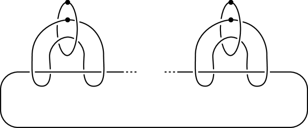
Figure 1. The Borromean knot $B_{2g}$. The dotted curves represent 1-handles (or 0-surgeries), see [GompfStipsicz].

Figure 2. The Borromean rings.

Definition 2.4.

Let $K$ be a link in a 3-manifold $M$, coloured by integers $i_{1},\dots,i_{c^{\prime}}$ and such that each colour appears at least once. Choose two components $K_{1},K_{2}$ of $K$ with the same colour, and knotify them, to get a coloured link $K^{\prime}\subset M\#S^{1}\times S^{2}$ with one less component than $K$. Iterate this procedure until you get a link $\kappa_{\rm col}(K)\subset M_{\rm col}$ with $c^{\prime}$ components, each coloured by an index $i_{1},\dots,i_{c^{\prime}}$. We call $(M_{\rm col},\kappa_{\rm col}(K))$ the coloured knotification of $K$

The following proposition formalises the construction of the attaching link $J$ of the $2$-handles of $N_{\mathcal{D}}$. The proof is omitted, as it is an easy adaptation of [BorodzikHeddenLivingston, Theorem 3.1] or [BCG1, Lemma 3.1].

Proposition 2.5.

The attaching link $J$ of the $c$ $2$-handles of $N_{\mathcal{D}}$ is the coloured knotification of the coloured connected sum of all links of singularities of $\mathcal{D}$ followed by a coloured connected sum with the $j$-coloured Borromean knot $B_{g_{j}}$ for $j=1,\dots,c$. The framing of the $j$-coloured component of $J$ (which is null-homologous in $\partial N^{1}_{\mathcal{D}}$) is $d_{j}^{2}$.

See Figure 3 for an example.

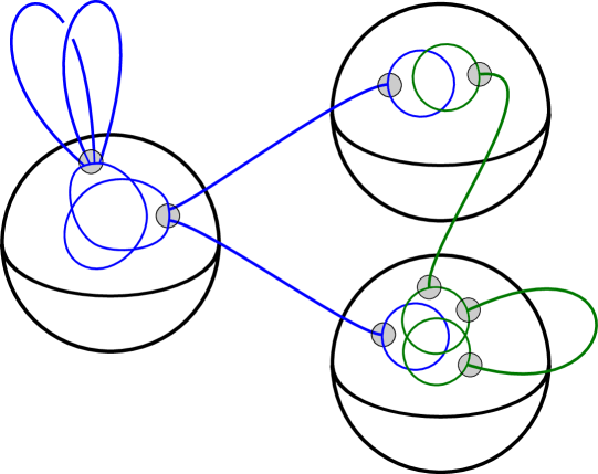
Figure 3. A schematic example of a handle decomposition of the neighbourhood of a reducible curve: here the curve has two components $C_{\rm b}$ and $C_{\rm g}$, and we colour the components of the links of their singularities by blue or green according to which curve they belong to. In the left-most ball, we see a trefoil and the two blue arcs represent a connected sum with a (blue) Borromean knot $B_{1}$, while the other blue components are unknots, so $C_{\rm b}$ has genus 1 and one simple cusp. In the bottom-most ball we see a green Hopf link, and the arc connecting its two components represents their knotification, so $C_{\rm g}$ has genus 0 and one singularity which is a simple node. $C_{\rm b}$ and $C_{\rm g}$ intersect at two points, which can be seen from the two balls on the right. On the top one we see a Hopf link, so $C_{\rm b}$ and $C_{\rm g}$ are non-singular and intersect transversely at that point. On the bottom ball we see a triple Hopf link (three fibres of the Hopf fibration), two green and one blue: this means that $C_{\rm b}$ and $C_{\rm g}$ intersect at the node of $C_{\rm g}$, in a generic way. The other arc connect the various coloured links along the corresponding curves. In this case, the result is a 2-component link in $(S^{1}\times S^{2})^{\#4}$.

2.2. Handle decompositions of complex curve complements

Recall that the complement of a complex curve is an affine complex surface, hence it is a Stein surface, and as such it admits a handle decomposition with handles of indices 0, 1, and 2. In a similar spirit, Libgober had given an explicit 2-dimensional finite CW complex with the same homotopy type as the complement [Lib1]. Very recently, Sugawara promoted Libgober’s cell complex to a handle decomposition of the complement. In this section, we briefly recall Sugawara’s work, which we will adapt to the symplectic context to prove the divisibility relations.

To fix the framework, we recall first the construction used to define the braid monodromy of a plane algebraic curve which allows to understand the topology of a (singular) plane curve, to find a representation of the fundamental group of its complement and to give an explicit handle decomposition of the latter (see [Mo, Lib1, Cohen] for more details).

Let $\mathcal{C}$ be an algebraic curve in $\mathbb{C}\mathbb{P}^{2}$ of degree $d$ with $\ell$ components. Let $L$ be a line at infinity. We denote by $\mathcal{C}^{+}=\mathcal{C}\cup L$. After a suitable change of coordinates, we may assume that $p=[0:0:1]$ belongs to $L$ but not to $\mathcal{C}$. Consider the linear projection from $p$, $\pi\colon\mathbb{C}\mathbb{P}^{2}\setminus L\to\mathbb{C}$. Let $\mathcal{Y}=\{y_{1},\dots,y_{s}\}$ be the set of points in $\mathbb{C}\mathbb{P}^{1}$ for which the fibers of $\pi$ contains at least one singular point of $\mathcal{C}$ or are tangent to $\mathcal{C}$. If each point $\pi^{-1}(y_{i})$ either contains a unique singularity of $\mathcal{C}$ or is simply-tangent to $\mathcal{C}$ at a single point for each $i$, we say that the projection $\pi$ is generic. For each $i$, let $\gamma_{i}$ be a loop based at $y_{0}\in\mathbb{C}\setminus\mathcal{Y}$ which goes counterclockwise around $y_{i}$ once does not wind around any other $y_{j}$ for $j\neq i$.

The fibers of $\pi$ are complex lines $L_{y}:=\pi^{-1}(y)\simeq\mathbb{C}$. If $y\not\in\mathcal{Y}$, then $L_{y}$ intersects $\mathcal{C}$ transversely in $d$ points. The map $\pi$ is a singular fibration $\mathbb{C}\mathbb{P}^{2}\setminus\mathcal{C}^{+}\to\mathbb{C}$, and its restriction to the complement of $\pi^{-1}(\mathcal{Y})$ is a locally trivial fibration

$$\mathbb{CP}^{2}\setminus(\mathcal{C}^{+}\cup L_{y_{1}}\cup\dots\cup L_{y_{s}})\to\mathbb{C}\setminus\mathcal{Y}$$

with fiber $F\cong\mathbb{C}\setminus\{1,\dots,d\}$. Since the mapping class group of $F$ (relative to the boundary at infinity) is the braid group $B_{d}$ on $d$ strands, the monodromy of this fibration is a morphism

$$\pi_{1}(\mathbb{C}\setminus\mathcal{Y},y_{0})\to B_{d},$$

which is called the braid monodromy of the curve $\mathcal{C}$ with respect to the line at infinity $L$. Concretely, this morphism takes the loop $\gamma_{i}$ to a braid describing the motion of the $d$ points in the intersection of the curve and the fibers as one moves along $\gamma_{i}$.

$\mathbb{D}$ at 10 10 $y_{0}$ at 84 24 $U_{1}$ at 18 83 $U_{2}$ at 51 118 $U_{s}$ at 167 67 $S_{1}$ at 59 36 $S_{2}$ at 71 52 $S_{s}$ at 124 36 $\ddots$ at 105 65 $\mathbb{D}$ at 212 10 $y_{0}$ at 286 24 $U_{0}$ at 310 18 $U_{1}$ at 220 83 $U_{2}$ at 253 118 $U_{s}$ at 369 67 $\nu(S_{1})$ at 252 32 $\nu(S_{2})$ at 293 75 $\nu(S_{s})$ at 331 32 $\ddots$ at 307 65

Figure 4. $\Gamma^{\prime}$ and its neighbourhood $\nu(\Gamma^{\prime})$ in $\mathbb{D}.$