Taming Landau level mixing in fractional quantum Hall states with deep learning
Abstract
Strong correlation brings a rich array of emergent phenomena, as well as a daunting challenge to theoretical physics study. In condensed matter physics, the fractional quantum Hall effect is a prominent example of strong correlation, with Landau level mixing being one of the most challenging aspects to address using traditional computational methods. Deep learning real-space neural network wavefunction methods have emerged as promising architectures to describe electron correlations in molecules and materials, but their power has not been fully tested for exotic quantum states. In this work, we employ real-space neural network wavefunction techniques to investigate fractional quantum Hall systems. On both and filling systems, we achieve energies consistently lower than exact diagonalization results which only consider the lowest Landau level. We also demonstrate that the real-space neural network wavefunction can naturally capture the extent of Landau level mixing up to a very high level, overcoming the limitations of traditional methods. Our work underscores the potential of neural networks for future studies of strongly correlated systems and opens new avenues for exploring the rich physics of the fractional quantum Hall effect.
The fractional quantum Hall (FQH) effect is one of the most notable examples in condensed matter physics, highlighting the fascinating emergent phenomena driven by strong correlation effects and non-trivial topology [1, 2]. In FQH systems, the kinetic energy is quenched by the strong magnetic field, and the Coulomb interaction dominates the physics. Consequently, the wavefunction of a FQH system can not be adiabatically connected to a simple, non-interacting state described by a single Slater determinant. This complexity, combined with their intriguing topological properties, makes it challenging to represent these ground states efficiently using conventional methods.
Early studies usually assume infinitely strong magnetic fields, confining all electrons to the lowest Landau level (LLL). However, in typical experiments, the Coulomb interaction strength is comparable to the cyclotron energy [3], and the Landau level mixing (LLM) can induce new physics. Recent experiments have linked LLM to phenomena such as Wigner-crystal phase transitions [4, 5], spin transitions [6], and novel non-Abelian FQH states [7, 8]. Nevertheless, traditional numerical approaches have limitations in addressing LLM. Exact diagonalization (ED) typically explicitly handles only the lowest Landau level (LLL) due to the large Hilbert space dimension [9], with very few studies extending it to two Landau levels [10]. Density matrix renormalization group (DMRG) method can include up to five Landau levels but struggles with states near the critical point with high entanglement [11, 12]. The fixed-phase diffusion Monte Carlo method (fp-DMC) is limited by the accuracy of its phase approximation and does not provide an explicit wavefunction [13, 14, 15].
In recent years, deep learning methods have emerged as promising alternatives for studying strongly correlated systems [16, 17]. These methods have achieved remarkable success in representing the wavefunctions of various strongly correlated systems, including lattice models [18, 19], molecules [20, 21, 22, 23, 24], solids [25, 26, 27], electron gases [27, 28, 29, 30], and Moiré systems [31, 32]. In these architectures, wavefunctions are presented in real space with neural networks, which can naturally include contributions from higher Landau levels within the ansatz. This capability makes deep learning based on real-space neural networks a promising tool to break through the limitations of traditional methods and gain deeper insights into the ground states of FQH systems with LLM.
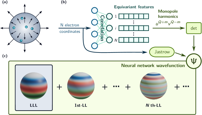
In this study, we employ real-space neural network methods to investigate FQH systems in spherical geometry [33]. In the literature, disk [2] and torus [34] geometries are also employed to study FQH effects, compared to which the spherical geometry has several advantages, including the edgeless structure, the well-defined filling factor and the simplicity in mathematical treatment. As shown in Fig. 1a, spin-polarized electrons are confined on a spherical surface, with a magnetic monopole placed at the center. The monopole creates a total flux of through the surface, where is the flux quantum and is an integer. The radius of the sphere is given by , where is the magnetic length, and is the strength of the uniform magnetic field on the sphere. The flux-particle relationship on the sphere is determined by , where is the filling factor and is the shift, which characterizes the topological properties of the corresponding FQH state [35].
The Hamiltonian on the spherical geometry is formulated as:
| (1) |
where is the cyclotron frequency, is the band mass of the electrons, is the dielectric constant of the material, and is the coordinate of the -th electron. is proportional to the canonical momentum tangential to the surface:
| (2) |
We define as a measure of the interaction strength, which also effectively tunes the LLM. All energies shown are in unit of .
Crafting a valid and expressive neural network wavefunction ansatz is essential for obtaining fractional quantum Hall states with deep learning. To achieve this, we design a trial wavefunction as follows:
| (3) |
where denotes the coordinates of all electrons, and the notation indicates that the permutation of other electrons does not change the output (Fig. 1b). The Jastrow factor
| (4) |
is included to satisfy the electron–electron Coulomb cusp condition [38], where is a free parameter. And the multi-electron orbitals on the sphere are given by
| (5) |
where are complex parameters and are monopole harmonics [39] on the LLL, with . The spinor coordinates of the -th electron are given by and . The use of monopole harmonics largely avoids the divergence problem in local energy at the poles of the sphere originating from Dirac strings, and the physical information such as the correlations and topological properties is encoded in the neural network . Here, the Psiformer neural network architecture [24] is adopted, which is capable of modeling strongly correlated electrons.
With the ansatz constructed, we then employ the variational Monte Carlo process to optimize the wavefunction. The loss function during training is chosen as the energy evaluated using Monte Carlo integration. The Kronecker-Factored Approximate Curvature method [40] is used to optimize the parameters. With the expressiveness of the neural network, it is possible to describe the quantum Hall states using a single determinant constructed with multi-electron orbitals . Moreover, the neural network wavefunction can naturally include the effects of LLM (Fig. 1c), surpassing the calculations that only include few Landau levels.
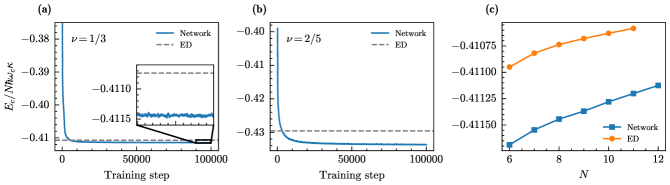
We first apply the neural network based variational Monte Carlo (NNVMC) to investigate the most robust FQH effect at , for which the Laughlin wavefunction provides a good description of the ground state [2]. A simulation containing electrons with flux and is shown in Fig. 2a. The energy obtained from the neural network reaches lower than the ED result, which only considers the LLL. This reflects the contribution of higher Landau levels due to the Coulomb interaction. We also use our approach to study the more complex system, for which the composite fermion wavefunction of Jain was known to be a good ansatz [41]. As demonstrated in Fig. 2b, although the neural network converges more slowly compared to the state, it still reaches a much lower energy than the ED result. This indicates that the real-space neural network captures electron correlations consistently and can be successfully applied to study FQH systems of different fillings.
To further validate the robustness of our approach, we examine the energy as a function of the number of electrons for the state. As shown in Fig. 2c, the neural network results from 6 to 12 electrons are consistently lower than the ED results. This demonstrates the neural network’s ability to accurately capture the ground state energies across different system sizes. Moreover, it is worth noting that the system with electrons is inaccessible to ED due to the exponentially growing Hilbert space. However, NNVMC can handle this larger system size and the results align well with the trend observed for smaller numbers of electrons. This further underscores the scalability and effectiveness of neural network methods in exploring larger FQH systems.
The above results are obtained with , where LLM is mild. We now investigate the system with electrons and varying to examine whether our neural network architecture is able to learn FQH states for different levels of LLM. As illustrated in Fig. 3a, for a weak interaction strength, , where the lowest Landau level is dominant, the energy obtained from NNVMC is slightly lower than the ED result. This shows that the neural network can reliably capture the contribution of higher Landau levels even when LLM is small. As increases, LLM becomes more pronounced and the contributions from higher Landau levels become more significant. Consequently, ED calculations considering only the LLL would significantly overestimate the energy, hence NNVMC can reach much lower energy than ED. As expected, the gap between NNVMC and ED increases monotonously as a function of LLM.
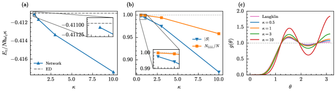
To further reveal the LLM effects, we monitor the overlap between the neural network wavefunction and the Laughlin wavefunction, which measures the similarity between them. The overlap is defined as:
| (6) |
In Fig. 3b, we plot the modulus of the overlap (). When is small, a large is obtained, since the Laughlin wavefunction is an excellent approximation of the ground state wavefunction in the absence of LLM. As LLM grows stronger, the modulus of overlap decreases, reasonably reflecting the influence of LLM.
The above results do not directly indicate whether the neural network wavefunction includes contributions from higher Landau levels. To gain deeper insights, we also examine the number of electrons on the LLL, denoted as . Our results in Fig. 3b show that follows the same trend as , being large at small and decreasing with larger . Although approximately 96% of the electrons remain on the LLL even at , the contribution from the remaining 4% of electrons in higher Landau levels is not negligible, as evidenced by the energy results. This highlights the significant role of higher Landau levels in the presence of LLM.
The neural network can also model the behavior of the pair correlation function (PCF) , which describes the probability of finding two electrons with an angular separation of and reveals the correlations between electrons. The FQH state is known to resemble a liquid [42], as illustrated by the PCF of the Laughlin wavefunction in Fig. 3c. The PCF from the neural network wavefunction closely matches that of the Laughlin wavefunction when . As LLM increases, the PCF becomes more structured. Eventually, at , the PCF no longer exhibits a decaying trend and displays a prominent peak at , indicating a phase transition away from the liquid phase [43, 44, 45]. However, the current system size in our approach is not sufficient to definitively establish the phase boundary. This is also evident in the subsequent energy gap calculations, where the charge gap persists up to , as shown in Fig. 4c. Nevertheless, the transition trend observed in our calculations aligns with the classical limit , where the system is known to form a classical Wigner crystal with electrons arranged in a triangular lattice [46, 47].
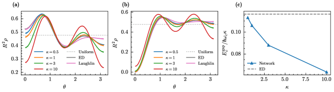
Besides the ground state, the corresponding quasiparticle and quasihole excitations in FQH systems also exhibit interesting physics. These excitations carry fractional electric charges, a remarkable departure from the usual integer charges, and they exhibit anyonic braiding statistics, which are neither bosonic nor fermionic. On the spherical geometry, the quasiparticle and quasihole states are actually ground states for different flux values . To reveal the charge density for these excitations, we need to break the degeneracy of different excitations by adding a penalty term to the loss function during the network training, where is the total angular momentum in the -direction, is the target , and is a tunable hyperparameter. The training is first converged with , and then we turn on to select the state whose . In Fig. 4a–b, we plot the charge density for quasiparticle and quasihole excitations from NNVMC for the system with , scaled by the square of sphere radius . Notably, since the Laughlin wavefunction captures short-range physics [33], the excitations are more localized compared to the ED and neural network results. For small , the neural network results agree well with the ED results, further demonstrating that our neural network wavefunction accurately captures the physics of the FQH system. As increases, the density fluctuations are enhanced compared to the ED results, consistent with the behavior of the PCF shown in Fig. 3c. At a large , the quasihole excitation density near the center is no longer close to zero, indicating a phase transition at high .
Having demonstrated the accuracy of neural network wavefunction, we can now study the transport gap of FQH systems and the effects of LLM on it, which are important topics that pose challenges to the theoretical community [48, 49, 50]. The transport gap corresponds to the energy cost of moving a quasiparticle far from the system, leaving a quasihole behind. This gap can be measured in finite-temperature transport experiments [51, 52]. It also reflects the composite fermion mass and can be deduced by the composite fermion Chern–Simons field theory [53, 54, 55, 56]. The transport gap is defined as , where and are quasiparticle and quasihole energies, respectively. Similar to Fig. 2, we denote the corrected gap as . As shown in Fig. 4c, for small values of , the transport gap aligns closely with the value obtained from ED. As increases, the transport gap decreases progressively. However, even at , the transport gap does not fully close, indicating that the system remains in a gapped phase despite the significant influence of LLM. These results are all consistent with previous studies [57, 58, 50].
In conclusion, we have demonstrated the effectiveness of deep learning methods in investigating FQH systems, capturing contributions from higher Landau levels. We employ the spherical geometry and examine the bulk properties and quasiparticle excitations of the and states, where we show that real-space neural networks can learn more accurate wavefunctions than those obtained by exact diagonalization based on the lowest Landau levels. In a concurrent study, a similar approach to this work is devised to study FQH on disk geometry, where similar conclusions were drawn, further highlighting the strengths of neural network methods [59]. Together with this work, these successes highlight the potential of neural networks for future explorations, including investigations into additional filling factors and other topological properties. Our results also show hints of the phase transition, but further investigations are desired to elucidate the issue. In the future, deep learning frameworks can be further designed to encode key physical information, which may lead to more efficient solutions and more advancements in addressing challenging questions resulting from strong correlations.
Acknowledgments
The authors would like to thank Nicholas Regnault, Jiequn Han, and Xi Dai for their helpful discussions, and ByteDance Research Group for inspiration and encouragement. J.C. acknowledges supports from the National Key R&D Program of China under Grant No. 2021YFA1400500, the National Natural Science Foundation of China under Grant No. 12334003, and the Beijing Municipal Natural Science Foundation under Grant No. JQ22001. T.X. acknowledges supports by the NSFC grant No. 12488201. T.Z. acknowledges supports by the China Postdoctoral Science Foundation grant No. 2023M743742.
References
- Stormer et al. [1999] H. L. Stormer, D. C. Tsui, and A. C. Gossard, Reviews of Modern Physics 71, S298 (1999).
- Laughlin [1983] R. B. Laughlin, Phys. Rev. Lett. 50, 1395 (1983).
- Sodemann and MacDonald [2013] I. Sodemann and A. H. MacDonald, Physical Review B 87, 245425 (2013).
- Goldman et al. [1990] V. J. Goldman, M. Santos, M. Shayegan, and J. E. Cunningham, Phys. Rev. Lett. 65, 2189 (1990).
- Thiebaut et al. [2015] N. Thiebaut, N. Regnault, and M. O. Goerbig, Phys. Rev. B 92, 245401 (2015).
- Eisenstein et al. [1989] J. P. Eisenstein, H. L. Stormer, L. Pfeiffer, and K. W. West, Phys. Rev. Lett. 62, 1540 (1989).
- Luhman et al. [2008] D. R. Luhman, W. Pan, D. C. Tsui, L. N. Pfeiffer, K. W. Baldwin, and K. W. West, Phys. Rev. Lett. 101, 266804 (2008).
- Wu et al. [2014] Y.-L. Wu, B. Estienne, N. Regnault, and B. A. Bernevig, Phys. Rev. Lett. 113, 116801 (2014).
- Regnault et al. [2017] N. Regnault, J. Maciejko, S. A. Kivelson, and S. L. Sondhi, Phys. Rev. B 96, 035150 (2017).
- Yoshioka [1984] D. Yoshioka, Journal of the Physical Society of Japan 53, 3740 (1984).
- Feiguin et al. [2008] A. E. Feiguin, E. Rezayi, C. Nayak, and S. Das Sarma, Physical Review Letters 100, 166803 (2008).
- Zaletel et al. [2015] M. P. Zaletel, R. S. K. Mong, F. Pollmann, and E. H. Rezayi, Physical Review B 91, 045115 (2015).
- Ortiz et al. [1993] G. Ortiz, D. M. Ceperley, and R. M. Martin, Physical Review Letters 71, 2777 (1993).
- Zhao et al. [2018] J. Zhao, Y. Zhang, and J. K. Jain, Phys. Rev. Lett. 121, 116802 (2018).
- Zhao et al. [2023] T. Zhao, A. C. Balram, and J. K. Jain, Phys. Rev. Lett. 130, 186302 (2023).
- Hermann et al. [2023] J. Hermann, J. Spencer, K. Choo, A. Mezzacapo, W. M. C. Foulkes, D. Pfau, G. Carleo, and F. Noé, Nature Reviews Chemistry 7, 692 (2023).
- Qian et al. [2024] Y. Qian, X. Li, Z. Li, W. Ren, and J. Chen, Deep learning quantum Monte Carlo for solids (2024), arXiv:2407.00707 [cond-mat, physics:physics] .
- Carleo and Troyer [2017] G. Carleo and M. Troyer, Science 355, 602 (2017).
- Vicentini et al. [2019] F. Vicentini, A. Biella, N. Regnault, and C. Ciuti, Phys. Rev. Lett. 122, 250503 (2019).
- Han et al. [2019] J. Han, L. Zhang, and W. E, Journal of Computational Physics 399, 108929 (2019).
- Pfau et al. [2020] D. Pfau, J. S. Spencer, A. G. D. G. Matthews, and W. M. C. Foulkes, Physical Review Research 2, 033429 (2020).
- Hermann et al. [2020] J. Hermann, Z. Schätzle, and F. Noé, Nature Chemistry 12, 891 (2020).
- Choo et al. [2020] K. Choo, A. Mezzacapo, and G. Carleo, Nature Communications 11, 2368 (2020).
- von Glehn et al. [2023] I. von Glehn, J. S. Spencer, and D. Pfau, in The Eleventh International Conference on Learning Representations, ICLR 2023 (OpenReview.net, kigali, rwanda, 2023).
- Yoshioka et al. [2021] N. Yoshioka, W. Mizukami, and F. Nori, Communications Physics 4, 1 (2021).
- Li et al. [2024a] X. Li, Y. Qian, and J. Chen, Physical Review Letters 132, 176401 (2024a).
- Li et al. [2022] X. Li, Z. Li, and J. Chen, Nature Communications 13, 7895 (2022).
- Wilson et al. [2023] M. Wilson, S. Moroni, M. Holzmann, N. Gao, F. Wudarski, T. Vegge, and A. Bhowmik, Physical Review B 107, 235139 (2023).
- Cassella et al. [2023] G. Cassella, H. Sutterud, S. Azadi, N. D. Drummond, D. Pfau, J. S. Spencer, and W. M. C. Foulkes, Physical Review Letters 130, 036401 (2023).
- Kim et al. [2024] J. Kim, G. Pescia, B. Fore, J. Nys, G. Carleo, S. Gandolfi, M. Hjorth-Jensen, and A. Lovato, Communications Physics 7, 148 (2024).
- Li et al. [2024b] X. Li, Y. Qian, W. Ren, Y. Xu, and J. Chen, Emergent Wigner phases in moiré superlattice from deep learning (2024b), arXiv:2406.11134 [cond-mat, physics:physics] .
- Luo et al. [2024] D. Luo, D. D. Dai, and L. Fu, Simulating moiré quantum matter with neural network (2024), arXiv:2406.17645 [cond-mat] .
- Haldane [1983] F. D. M. Haldane, Phys. Rev. Lett. 51, 605 (1983).
- Yoshioka et al. [1983] D. Yoshioka, B. I. Halperin, and P. A. Lee, Phys. Rev. Lett. 50, 1219 (1983).
- Wen and Zee [1992] X. G. Wen and A. Zee, Physical Review Letters 69, 953 (1992).
- Jain [2007] J. K. Jain, Composite Fermions, 1st ed. (Cambridge University Press, Cambridge ; New York, 2007).
- Morf et al. [1986] R. Morf, N. d’Ambrumenil, and B. I. Halperin, Phys. Rev. B 34, 3037 (1986).
- Kato [1957] T. Kato, Communications on Pure and Applied Mathematics 10, 151 (1957).
- Wu and Yang [1976] T. T. Wu and C. N. Yang, Nucl. Phys. B 107, 365 (1976).
- Martens and Grosse [2015] J. Martens and R. Grosse, in Proceedings of the 32nd International Conference on Machine Learning (PMLR, 2015) pp. 2408–2417.
- Jain [1989] J. K. Jain, Phys. Rev. Lett. 63, 199 (1989).
- Kamilla et al. [1997] R. K. Kamilla, J. K. Jain, and S. M. Girvin, Physical Review B 56, 12411 (1997).
- Yannouleas and Landman [2003] C. Yannouleas and U. Landman, Phys. Rev. B 68, 035326 (2003).
- Yannouleas and Landman [2002] C. Yannouleas and U. Landman, Phys. Rev. B 66, 115315 (2002).
- Shibata and Yoshioka [2001] N. Shibata and D. Yoshioka, Phys. Rev. Lett. 86, 5755 (2001).
- Thomson [1904] J. J. Thomson, Phil. Mag. 7, 237 (1904).
- E. Wigner [1934] E. Wigner, Phys. Rev. 46, 1002 (1934).
- Haldane and Rezayi [1985] F. D. M. Haldane and E. H. Rezayi, Phys. Rev. Lett. 54, 237 (1985).
- Morf et al. [2002] R. H. Morf, N. d’Ambrumenil, and S. Das Sarma, Phys. Rev. B 66, 075408 (2002).
- Zhao et al. [2022] T. Zhao, K. Kudo, W. N. Faugno, A. C. Balram, and J. K. Jain, Phys. Rev. B 105, 205147 (2022).
- Boebinger et al. [1985] G. S. Boebinger, A. M. Chang, H. L. Stormer, and D. C. Tsui, Phys. Rev. Lett. 55, 1606 (1985).
- Du et al. [1993] R. R. Du, H. L. Stormer, D. C. Tsui, L. N. Pfeiffer, and K. W. West, Phys. Rev. Lett. 70, 2944 (1993).
- Halperin et al. [1993] B. I. Halperin, P. A. Lee, and N. Read, Phys. Rev. B 47, 7312 (1993).
- Murthy and Shankar [2003] G. Murthy and R. Shankar, Reviews of Modern Physics 75, 1101 (2003).
- Yu et al. [1998] Y. Yu, Z.-B. Su, and X. Dai, Phys. Rev. B 57, 9897 (1998).
- Praz [2007] A. Praz, Phys. Rev. B 75, 205342 (2007).
- Melik-Alaverdian and Bonesteel [1995] V. Melik-Alaverdian and N. E. Bonesteel, Phys. Rev. B 52, R17032 (1995).
- Murthy and Shankar [2002] G. Murthy and R. Shankar, Physical Review B 65, 245309 (2002).
- Teng et al. [2024] Y. Teng, D. D. Dai, and L. Fu, Solving and visualizing fractional quantum Hall wavefunctions with neural network (2024), arXiv:2412.00618 [cond-mat] .
- [60] DiagHam, https://nick-ux.org/diagham.
- Fishman et al. [2022] M. Fishman, S. R. White, and E. M. Stoudenmire, SciPost Phys. Codebases , 4 (2022).
*
Appendix A Appendix: methodological and computational details
A.1 The role of monopole harmonics
It is mentioned in the main text that LLL monopole harmonics are used to avoid the divergence issue near the poles. The monopole harmonics handle the complex phases arising from the Dirac string, while the neural network encodes the correlations between electrons.
To understand it, let us first consider the case without the Dirac string, where divergences in local energy near the poles also exist. Consider a wavefunction near the north pole. To avoid divergence in local energy, the condition must be satisfied. Similarly, this condition must also hold near the south pole. While a neural network wavefunction may not strictly satisfy this relation, it is generally not a significant problem in practice. That is because the wavefunction should vanish rapidly near the poles as increases, contributing negligibly to the Monte Carlo sampling and the total energy.
With the Dirac string, the condition near the north pole becomes , and near the south pole, it becomes . A neural network wavefunction may not satisfy this relation, not to mention the singularities with ill-defined phases at the poles when . Moreover, examining the monopole harmonics reveals that orbitals with more complex phases (i.e., larger ) contribute more significantly near the poles. This means the neural network must precisely capture the complex phase in these regions. Additionally, since the largest is proportional to for a fixed filling, the phase becomes even more complex and challenging to learn compared to the case, where the largest is proportional to . By including LLL monopole harmonics in our neural network wavefunction, the complex phases of the wavefunction arising from the Dirac string can be properly handled.
A.2 Neural network architecture
In the neural network, , the input feature vector for the electron is chosen as the Cartesian coordinates of the electron:
| (7) |
The input features are then mapped to the attention inputs by a linear projection . After that, is passed though a sequence of multi-head attention layers and fully connected layers with residual connection:
| (8) |
| (9) |
where indexes neural network layers and indexes heads of the attention layer. And the standard self-attention is defined as:
| (10) |
| (11) | |||
| (12) |
where is the output dimension of the key and query weights. The hyperparameters of the neural network used in this study are listed in Table S1.
A.3 Energy corrections
The energy results shown in the main text include the contribution from background charge,
| (13) |
In addition, we shift the energy by and apply a density correction to reduce the dependence of the energy on the system size. The corrected energy is then defined as:
| (14) |
Notably, the background contribution to the excited states differs from that of the ground state. Specifically, for the state, these contributions are given by:
| (15) |
where corresponds to the excess charge in the excited states. And the transport gap after correction is essentially
| (16) |
A.4 Computational details
Overlap with Laughlin wavefunction —
The Laughlin wavefunction for state on a sphere is given by:
| (17) |
where and are the spinor coordinates of the -th electron, and is an odd integer. The overlap between the neural network wavefunction and is defined in Eq. (6). Given the two wavefunctions are similar, the overlap can be efficiently sampled using importance sampling from the distribution , expressed as:
| (18) |
where denote the expectation value under the distribution .
The number of electrons on the lowest Landau level
can be calculated using the trace of the one-body reduced density matrix (1-RDM), with the basis consisting of LLL monopole harmonics . The 1-RDM for wavefunction is defined as:
| (19) |
In practice, importance sampling based on the distribution is applied for the integral over , and uniform sampling is used for . Assuming the monopole harmonics are normalized, the integral in Eq. (19) can be calculated with:
| (20) |
The pair correlation function
is defined as:
| (21) |
where is the electron density on the sphere. Since on the spherical geometry, the PCF depends only on the angular separation between electrons and . Therefore, we can express the PCF as:
| (22) |
We approximate the function as:
| (23) |
where is the number of bins, and with . Therefore, in Monte Carlo simulations, we collect in bins with weight , and multiply by an overall factor:
| (24) |
ED calculations
of energy are performed using the DiagHam library [60]. The density profiles of quasiparticle and quasihole excitations are obtained by DMRG calculations in the LLL using the ITensor library for technical convenience [61]. We have verified that the energy values calculated by DMRG are identical to those obtained from DiagHam and the entanglement entropy is also converged to machine precision. These facts guarantee that the results from DMRG calculations are equivalent to ED calculations.