Dynamical Cavity Method for Hypergraphs and its
Application to Quenches in the -XOR-SAT Problem
École polytechnique fédérale de Lausanne (EPFL) CH-1015 Lausanne )
Abstract
The dynamical cavity method and its backtracking version provide a powerful approach to studying the properties of dynamical processes on large random graphs. This paper extends these methods to hypergraphs, enabling the analysis of interactions involving more than two variables. We apply them to analyse the -XOR-satisfiability (-XOR-SAT) problem, an important model in theoretical computer science which is closely related to the diluted -spin model from statistical physics. In particular, we examine whether the quench dynamics – a deterministic, locally greedy process – can find solutions with only a few violated constraints on -regular -uniform hypergraphs. Our results demonstrate that the methods accurately characterize the attractors of the dynamics. It enables us to compute the energy reached by typical trajectories of the dynamical process in different parameter regimes. We show that these predictions are accurate, including cases where a classical mean-field approach fails.
1 Introduction
The past decades have seen an explosion of applications of methods from statistical physics to study constraint satisfaction and optimization problems. In particular, the cavity method has shown to be remarkably well-suited to find equilibrium properties in the thermodynamic limit for systems from theoretical computer science [1, 2]. However, many questions relevant to optimization problems concern the performance of different algorithms – the dynamical processes on the graph, rather than the static properties of its energy landscape.
The cavity method conducts only a static analysis on the existence of solutions for a particular system. While this analysis has some implications for a specific group of algorithms [3], it does not concern other classes of simple search algorithms. The absence of exact solutions to this type of question led to the development of methods that take full trajectories of the dynamics account, namely the dynamical cavity method (DCM) [4, 5, 6, 7, 8], and more recently its backtracking version (BCDM) [9].
In the context of these developments, the first key contribution of this work is to present a generalization of both methods to the study of processes involving interactions between more than two variables, i.e. dynamical processes on hypergraphs. This is useful, because hypergraphs provide a general framework to represent constraint satisfaction problems with a wide range of applications including scheduling and location problems [10, 11, 12, 13].
As a direct application of this generalization, we consider the sparse -XOR-satisfiability (-XOR-SAT) problem, a variant of the classical Boolean satisfiability problem (-SAT) [14]. In -XOR-SAT, boolean variables are subject to constraints represented by XOR (exclusive OR) relations each involving variables. This is closely related to the diluted -spin model in statistical physics. For this reason, the problem gathered great interest in the field of disordered systems [15, 16, 17, 18].
Although the case of the diluted -spin model already offers a model with interesting properties (e.g. as the Ising or Sherrington-Kirkpatrick model), models with exhibit a more complex and rugged energy landscape. In particular, these are the prototypical models exhibiting the random-first-order type of phase transition with dynamical and Kauzmann transitions that were used to study the properties of more general glassy systems [19, 20].
While the evolution of simple algorithms was already analyzed for the case in [9, 21], in this work, we extend this analysis to the richer landscape of the -XOR-SAT (diluted -spin) model. More concretely, using the DCM and the BDCM, we seek to understand the convergence behavior of quench dynamics on -XOR-SAT instances and evaluate their performance in minimizing the number of unsatisfied constraints. In our context, a quench corresponds to a deterministic, synchronous and locally greedy evolution of the system from a highly entropic state to a low-energy out-of-equilibrium configuration. We use this dynamical process as a simple search algorithm and we compare its performance to the equilibrium properties of the system, i.e. the satisfiability threshold and spin glass phase transition [15, 22, 23].
In the remainder of this work, we first develop the notation of general dynamical processes on hypergraphs in Section 2, and for the -XOR-SAT problem in particular in Section 3. The dynamical cavity and its backtracking generalization to hypergraphs are introduced in Section 4, along with refinements for the -XOR-SAT. Together with a comparison to a naïve mean-field approach, we apply these methods to the -XOR-SAT and discuss our findings in Section 5.
2 Analysing Dynamical Processes on Hypergraphs
2.1 Notation
Hypergraphs.
We define an undirected hypergraph as a pair where are the nodes of the hypergraph and the hyperedges each contain a subsets of nodes, . There are hyperedges. When the context allows, we denote nodes using the letters and hyperedges with . The degree of a node , denoted , is the number of hyperedges that contain it, . Similarly, the order of a hyperedge is the number of nodes it contains, . The neighborhood of a node is the set of hyperedges that contain , formally . In this work we focus on regular and uniform hypergraphs: In a -regular hypergraph all nodes have the same degree and in a -uniform hypergraph all hyperedges have the same order . We note that a 2-uniform hypergraph is an ordinary graph, where hyperedges are called edges and each edge is a link between two nodes.
Dynamics.
In the case of a time discrete dynamical process on a -regular and -uniform hypergraph, each node is assigned, at each time step from time until , one of the discrete states from a finite set . We denote the state of node as and the states of all nodes belonging to a subset as . The state of the complete hypergraph, the configuration, is given by the vector .
The dynamical process is described by a map , the global update rule, that gives the configuration at the next time step as a function of the current configuration, . Under the assumption that the next state of a node only depends on its current state and the states of the nodes contained in its neighborhood, can be written as a set of local update rules such that . Note that in this process, the update of the nodes is synchronous, deterministic and independent of the order of the neighbors.
Since a hyperedge represents an interaction between nodes, in this paper we decompose the local update rule as:
| (1) |
where the output of can be seen as the preference of hyperedge for the next value taken by node , and aggregates all received inputs from its edges to update . This representation allows us to treat the influence of a node on the update of as part of the preference of the hyperedge . The introduction of the inner local update rule removes part of the information accessible to the node , as the individual values of the nodes in the neighboring hyperedges are no more known. It restricts the space of update rules that can be written in this framework.
A trajectory of length t is defined as a trajectory of configurations with the additional constraint that for all . Additionally, a sequence such that is called a limit cycle or attractor of length c. Since the configuration space is finite and the update rule is deterministic, the discrete temporal evolution of any initial configuration is guaranteed to eventually reach either a stable configuration , or a limit cycle . Note that a stable configuration is a limit cycle of length . When considering a trajectory , where is an attractor, the part of the trajectory preceding the attractor, is called the transient, with transient length . All configurations that converge to the same attractor are said to form its basin of attraction.
The transition graph of the dynamical process on a given graph is the directed graph where every configuration of the original graph is a node: . There exists a directed edge if and only if the transition exists.
2.2 Analyzing the Dynamics
The goal of this work is to analyze the properties of the dynamical process. Some of the questions we are interested in are: What are common properties of the basin of attraction of a given type of attractor? How are the limit cycles of the dynamical process composed, e.g. are they homogeneous and take the same value? What size do the limit cycles have?
Dynamical transition graph motifs.
We want to answer these questions through the main object of this work’s analysis, the backtracking attractor, a dynamical motif of the update functions transition graph defined on the set of all possible configurations.
Concretely, we define a backtracking attractor to be a trajectory
| (2) |
with an incoming path of length ending in a limit cycle of length , following the formalism introduced in [9]. This is a dynamical motif in the transition graph . Note that we may also set to select paths without constraining them to a cycle. This is known as the (forward) dynamical cavity method [7]. We may also set to individually analyze the limit cycles, as previously done for dense graphs by [24].
The properties of the process we are interested in are translated into the observables, which are functions of backtracking attractors that return a scalar value. We define them as an intensive quantity in the graph size which factorizes on the nodes, , or on the edges, , as
| (3) | ||||
| (4) |
where all functions map to a single scalar value and may be specific to a given node or edge (via dependence on ). Concretely, a node observable could measure the prevalence of a given state at initialization, or in the limit cycle. An edge observable could quantify whether an edge contains nodes that are all in the same state or not.
In the following, the goal of our analysis is to quantify how many backtracking attractors are contained in the transition graph for a given graph and a dynamical process . Observables can be used to both condition the backtracking attractors that we take into account on a given value, and to measure a given observable for a selected subset of those backtracking attractors. As an example, one could aim to find the average initialization (measured observable) of processes that end up in a homogeneous state (conditioned observable) after 5 steps (setting ).
Measuring backtracking attractors.
In order to count the prevalence of the given backtracking attractors in a transition graph, we define a probability distribution over the dynamical motifs which only takes into account valid distributions and weighs them according to the observable of interest.
Concretely, for a given graph of size , update rule and natural numbers , we introduce a probability distribution over all trajectories of size , , with:
| (5) |
Only a trajectory that is coherent with the update rule and ends in a limit cycle of length has a non-zero measure in this distribution – precisely a backtracking attractor. The partition function is introduced to normalize the distribution . When we neglect the boundary condition, the first factor in (5), and give non-zero measure to all trajectories of length . Finding the partition function, or equivalently the free entropy density , amounts to counting the number of valid backtracking attractors.
Beyond counting how many backtracking attractors exist for a given our analysis also allows to measure and condition on observables (4) of the attractors. To do so, we introduce them as flexible constraints, re-weightings of the probability distribution, in the form of Lagrange multipliers in the distribution (5), with one multiplier per observable. For example, the partition function of the modified distribution for a set of observables with intensive properties reads:
| (6) |
We define the entropy of a class of backtracking attractors as . The term is the number of backtracking attractors in the transition graph. As we take the graph size to infinity, we can apply the saddle point method to yield
| (7) | ||||
| (8) |
which gives the free entropy density as
| (9) | |||
| (10) |
From (9), as the observables concentrate around:
| (11) |
Here, denotes the average over the distribution . If one can compute and for a given set of , then obtained from (9) gives the entropy of the class of backtracking attractors defined by the constraints , . The same holds for observables defined on the edges, if the edges scale as a constant fraction in the number of nodes.
By setting it is possible to measure the value of the observable without constraining it. In other words, is the value of the observable that is most likely to be observed in a typical trajectory of the dynamical process whose transient length is smaller or equal to and limit cycle length is a divisor of .
While these quantities are defined easily mathematically, computing the exponential sum in the partition function in (6) is computationally infeasible. Hence, we will introduce the cavity method later on which approximates the free entropy density in a manner that is exact in the leading order for large random hypergraphs. Before this, we turn to the -XOR-SAT problem and its interesting properties for motivation.
3 The -XOR-SAT Problem and Quench Dynamics
The main focus of this work is a special subclass of dynamical processes on graphs. These processes on the graphs relate both to the -XOR-SAT problem and the diluted (sparse) -spin problem. The dynamics are such that each node synchronously chooses a state that satisfies the desired properties of the global problem – but only based on its local neighborhood. Fixed points of the dynamical process are solutions to the problem. Our goal is to determine when these fixed points are (not) reached and how long this typically takes when we initialize the dynamical process at random instances of the problem.
3.1 The -XOR-SAT / diluted -spin Problem
We consider the special case of hypergraphs where the nodes take two possible states . Every node represents a boolean variable, where we take to be true and to be false. We interpret each hyperedge that connects a number of such nodes as a logical expression, a clause. For a given configuration , we attribute a truth value to each hyperedge, which is the structure equivalent to a clause in XOR-SAT. The goal is to have all clauses satisfied.
Problem Statement.
We consider the case where a hypergraph edge takes the parity of the incoming variables as
| (12) |
Here, we can view as the desired parity of the interaction, a property that is local to the hyperedge . To each configuration , we attribute an energy value which relates to the number of unsatisfied clauses using the following energy density:
| (13) |
which takes values in . This definition corresponds to setting a satisfied clauses value at and each unsatisfied clause at , and normalizing by the number of hyperedges in the graph. When we consider -regular and -uniform graphs we have . It is if all clauses are satisfied. When it is possible to find a configuration which takes value , we say that the problem is satisfiable for a given graph and constraint set .
Note that our formulation of the problem does not incorporate variables that appear negated in a clause, so this formulation does not incorporate every possible XOR-SAT problem. However, universality results along the lines of [25] imply that the results we obtain also have close implications for the versions of the -XOR-SAT problem where variables are randomly negated in clauses.
Related Formulations.
For -regular and -uniform graphs, this class of problems is known in statistical physics as the diluted -spin model. Here, corresponds to in our notation, and diluted highlights that the analysis is for sparse graphs – is constant in . More specifically, the cases of different distributions over are known as
| spin-glass | for uniformly at random, |
|---|---|
| ferromagnet | for everywhere, |
| anti-ferromagnet | for everywhere. |
Static Properties.
For even values of , the conjecture introduced in [25] suggests a universality between all three formulations. It was found that -XOR-SAT instances are satisfiable with high probability when the ratio is greater than [22]. When is odd, note that there is a trivial ground state (configuration that minimizes the energy density) for the ferromagnet with (anti-ferromagnet with ) by setting all nodes to (). In both cases, the non-trivial transition energy between the Replica Symmetric phase (RS) and the 1-step Replica Symmetry Breaking (1RSB) is in agreement with the result of the spin glass model. The former is shown in Appendix B, and the latter was computed in [26]. This allows us to further argue in favor of equivalence between the two models both for even and odd values of , apart from the trivial () configuration. Instead of analyzing the static properties, in the following we turn to the analysis of a specific algorithm: The quench.
3.2 Synchronous Quenched Local Updates
We consider the quench dynamics on -XOR-SAT instances. The idea is that this process behaves as a local greedy algorithm seeking to minimize the energy of the system. A quench corresponds to a system that is initialized at a high temperature and abruptly cooled down to zero temperature. It then evolves in a greedy and synchronous way to locally minimize the energy, until it reaches a local minimum or limit cycle, hence the name for the dynamics we investigate.
The update function.
At initialization , the configuration of a given hypergraph is chosen with every node taking values uniformly at random. Each node is then updated to locally maximize the number of satisfied clauses based on the current configuration. To do so, we set
| (14) |
This inner local update rule returns the value of that would satisfy the clause given that all other nodes where kept constant. Since every node appears in several clauses, we aggregate the preferences over every individual clause via a majority voting mechanism. This aggregation mechanism is defined as
| (15) |
Adding the current value of in the sum allows to break ties in favor of the current value of the node.
Specific observables.
In Section 2.2 we described how observables of the system can help to characterize different dynamical processes. In the case of the quench dynamics on the -XOR-SAT we ask whether we can reach a low-energy configuration, what the attractors of the system look like, and how this depends on the initialization. Defining a backtracking attractor of the dynamical system as on a hypergraph with nodes and hyperedges, we investigate the following observables:
In the remainder of this work we refer to nodes that change during a limit cycle as rattlers.
4 Dynamical Cavity Method for Hypergraphs
This section introduces the backtracking dynamical cavity method for the analysis of dynamical processes on hypergraphs, as a tool to study the evolution and convergence behavior of the system. Using this method, we can derive closed-form equations that predict the observables for a given update function in a high-dimensional limit, where the number of nodes grows to infinity for constant and .
In Section 2.2 we showed that the entropy obtained from (9) gives a measure of the number of trajectories that converge in or fewer steps to an attractor of given period . In the limit , this set of trajectories represents the basin of attraction of length- limit cycles. By measuring observables on this basin of attraction, we aim to extract information about the dynamics of the process and its attractors. At the same time, by only considering paths with , i.e. not constraining them to end in cycles, we can explore the start of the dynamics from a random typical configuration and measure observables. However, computing both the entropy and the observables directly is infeasible since it involves high-dimensional sums over the space of all possible graph configurations.
In this section, we show how to apply the cavity method [27] to the distribution of backtracking attractors to approximate the free entropy density on a hypergraph. The idea of this method is to factorize the probability distribution from Section 2.2 on the underlying graph structure and to then compute an approximation of the complete distribution via local message passing.
For this is known as the dynamical cavity method (DCM) and was introduced in its forward version in [4, 5, 6, 7, 8]. The backtracking dynamical cavity method (BDCM) was developed in [9] to consider backtracking attractor with , which was inspired by work aiming to find variable-length limit cycles [24]. In all cases, these methods were defined for simple graphs – in this work we extend them to the more general setting of hypergraphs.
4.1 General Hypergraphs
For the cavity method to be applicable, the distribution must factorize on a graph. We assume that all observables of interest can be written as a sum of local variables depending on a single edge, or a node and its neighborhood, as shown in (4). Then, assuming there is one node observable and one hyperedge observable , the factorized probability distribution from (5) reads:
| (16) |
Here, regroups the constraints and observables factorized on the nodes and those factorized on the hyperedges for two Lagrangian parameters :
| (17) | ||||
| (18) | ||||
| (19) |
where is a shorthand notation for . The factorized probability distribution (16) can be represented on a factor graph, where the nodes are the variable nodes and the hyperedges are factor nodes with function . Additional factor nodes are introduced to represent the constraints and observables factorized on the nodes, with function . Note that it is possible to add more observables on the nodes or the hyperedges if needed.
Removing short loops.
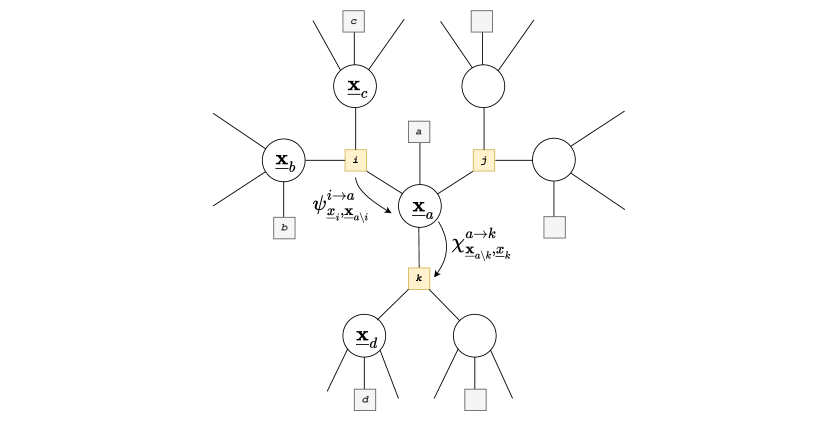
If the underlying factor graph is a tree, applying the cavity method to this distribution allows one to exactly compute the properties of the distribution, such as its marginals and entropy. If the graph is similar to a tree, in the sense that it only contains large loops (logarithmic in the system size ), the cavity method has been shown to give accurate measurements. However, in the representation selected before, any two nodes belonging to a same hyperedge are connected in the factor graph both through their respective factor nodes and , and through the factor node . This results in short loops of length four. This issue can be resolved by considering the hyperedges of the hypergraph as the variable nodes containing the values of all nodes belonging to the hyperedge. This modified factor graph architecture was similarly used in [28, 29, 9] to obtain a regular factor graph. Now, the nodes are written as factor nodes with function and an additional factor node with function is added to each variable node . This factor graph is shown in Fig. 1.
Message Passing.
The Belief Propagation (BP) equations corresponding to the probability distribution (16) then read:
| (20) | ||||
| (21) |
Once they have converged, the BP messages and can be used to compute an approximation of free energy density under the factorized model. We call this Bethe free entropy density to highlight that it was obtained under the replica symmetric assumption, i.e. under the assumption that the probability distributions over trajectories can be locally represented via belief propagation.
| (22) | ||||
| (23) | ||||
| (24) | ||||
| (25) |
Iterating the BP messages on a given graph, allows one to find a fixed point, for which the above Bethe free entropy can be evaluated.
4.2 The case of -regular, -uniform hypergraphs
In the case of a -regular -uniform hypergraphs with update functions and , we assume that the probability distributions over the messages are independent of the concrete neighbourhood of node . Likewise, we assume that all observable functions and are independent of the respective node or edge. Note that for the -XOR-SAT problem this is the case only when we consider the (anti-)ferromagnetic case with constant in , and not the spin-glass. Hence, we assume that all BP messages become the same and can be iterated on a single node. By loosing this dependence, the equations for the messages are simplified as
| (26) | ||||
| (27) |
where the are defined to be tuples of size configurations, representing a neighborhood. Likewise is a single configuration. By the we mean that we take away the ’th element of a tuple. These equations in turn lead to the Bethe entropy, where now represents a -tuple instead, as
| (29) | ||||
| (30) | ||||
| (31) | ||||
| (32) |
The goal is now to find the fixed point of the messages again, which can be done by initializing randomly and then iterating the equations. From (26) and (27), we observe that the number of values that need to be iterated at each step is . The complexity of iterating one value of scales as . The complexity of this operation can be reduced by noting that the update rules are independent of the ordering of both the hyperedges in the neighborhood of a node and the other nodes in a hyperedge. The sum in (27) can therefore be computed using a dynamical programming algorithm [30]. This reduces the complexity of iterating one value of to . This leads to an algorithm for solving the equations iteratively, which takes . This is tractable for small values of , and .
4.3 A computational simplification for -XOR-SAT
We want to apply this method for update functions which represent the -XOR-SAT problem introduced in Section 3. The specific problem allows for a further computational simplification: We can achieve an iteration cost of which is no longer exponential in the hyperedge size .
Note that we can reformulate the -XOR-SAT problem in a way such that the hypergraph can be interpreted as an ordinary graph where hyperedges are a different type of nodes taking value and edges connect the nodes to the hyperedges to which they belong.
The update of the graph is no longer done in a single step but takes place in two sequential steps (since the graph is bipartite over the two node types):
| (33) | ||||
| (34) |
where is a function that maps from a neighborhood of size to a value in . Notation-wise, note that we have , and . Again, an underline considers the full trajectory over states. Under this new formalism, (16)-(19) become:
| (35) | ||||
| (36) | ||||
| (37) |
Similarly to the previous section, the factor graph representation of the probability distribution contains loops of length 4, due to the fact that any couple of a node and a hyperedge in its neighborhood are connected through both their respective factor nodes and . This issue is again solved by moving to the dual representation of the factor graph, taking the edges to be the variable nodes. In our representation, this results in the variable nodes being the tuples of a node and a hyperedge to which it belongs and each node and hyperedge being a factor node. The factor graph can be observed in Fig. 2.
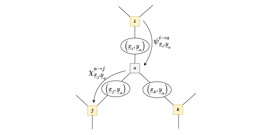
BP equations can be written from this factor graph, using four different types of messages: two between variable nodes and factor nodes representing nodes and two between variable nodes and factor nodes representing hyperedges . However, the messages and , as well as and , can be contracted to give the following compact BP equations:
| (38) | ||||
| (39) |
The free entropy density can then be computed using the BP messages as:
| (40) | ||||
| (41) | ||||
| (42) | ||||
| (43) |
and the simplified equations in the case of a -regular -uniform hypergraphs with update functions and that are independent can be written as:
| (44) | ||||
| (45) |
where is a tuple of trajectories and is a tuple of trajectories of . To write the entropy density, we slightly modify this notation to say that now and are and tuples of and respectively:
| (46) | ||||
| (47) | ||||
| (48) | ||||
| (49) |
We conclude that in this setting the number of messages to be updated at each step has been reduced to and, using a dynamical programming scheme to optimize the sums over and in (45) and (44). This amounts to for a single iteration. The exponential term in was reduced to a polynomial.
5 Application to Quenches in -XOR-SAT
In this section, we present results to characterize the evolution and convergence behavior of quench dynamics in -XOR-SAT instances through the DCM and BDCM. We evaluate them based on their agreement with numerical simulations and compare them to the naïve mean-field approach, presented in Appendix A. The code used to compute the BDCM and DCM results, the numerical simulations, and the mean-field predictions are available publicly at https://github.com/SPOC-group/k-xorsat-bdcm.
We have two principal questions that we want to answer for dynamics that are initialized at random: How fast do the dynamics reach a steady state or an attractor? What is the energy of the attractors they reach?
5.1 General Phenomenology
Depending on the degree and uniformity of the underlying graph, the behavior exhibited by the quench dynamics introduced in Section 3 is quite different. From here on, we examine the anti-ferromagnetic case, where . For this, we can use the simplified and more efficient factor graph from Section 4.3. For an overview of the different dynamical processes, Table 1 groups different values of together when we find empirically that their behaviour is similar. In particular, we distinguish even and odd degrees of , and within the odd degrees we further distinguish between small and large hyperedge sizes .
| Transient length as | Typical limit cycle as | To be noted | ||
|---|---|---|---|---|
| even | any | 1-cycles (larger cycles with vanishing fraction of rattlers as ) | behaviour of graphs generalizes to hypergraphs | |
| odd | 2-cycles with average zero energy | |||
| large cycles that grow in | singular case with linear cycle length | |||
| difficult to analyze empirically due to long convergence time |
5.2 Averaging the System: A Mean Field Approach
One of the most common methods to analyse a dynamical process is a mean-field approach. The key idea is to replace the interactions between individual elements of the system with the average interactions of the whole system. The hope is that this ansatz holds true when the system is large enough. In the case of sparse -XOR-SAT, it is possible to apply this principle to the values defined on the hyperedges, and to update them in terms of the average probability of a given value for the whole graph, rather than in terms of the local interactions. This leads to a prediction of the evolution of the energy of the process. In Appendix A we describe the simple iterative update equations that we derive from this principle in detail.
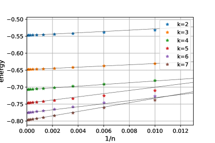
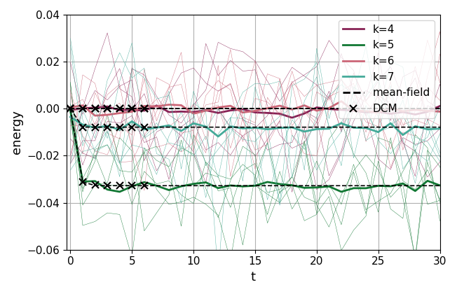
Fig. 3 shows how the empirical evolution of 5 different samples of graphs evolves over time , for different . We compare this with the prediction of the mean field approach, in solid lines. During the first few timesteps the empirics and the mean field projections match closely. However, at some point the prediction diverges from the empirics as it reaches the homogeneous fixed point. For many processes we examine here this mean-field fixed point is far off the actual fixed point that the process reaches empirically. This is not surprising as it does not incorporate enough knowledge of the correlation structure between neighboring nodes that builds up over the course of the process. In the following, we investigate the dynamical cavity methods and show that this method obtains more accurate predictions since it incorporates these correlations. We conjecture that in the large size limit of random hypergraphs, these methods capture all the correlations that influence leading order behaviour unless replica symmetry is broken, for which we have not observed any evidence in the studied problem. We examine both the forward analysis, as well as the backtracking one.
5.3 The Beginning of the Process: Forward Dynamical Cavity Method
The DCM is more accurate than the mean field.
Fig. 3 shows the numerical evolution of the energy of the quench dynamics on hypergraphs of degree with hyperedges of varying size. We compare the mean-field prediction for the energy and the results of the DCM, computed from (11) after convergence of the BP messages for the first steps of the dynamics. The exponential dependency of the BP equations (44)-(45) on the length of the trajectory prevents us from obtaining numerical DCM results for . Nonetheless, this suffices to show that the DCM accurately follows the numerical trajectories whereas the mean-field approximation already diverges. With more computational power, this prediction could be continued over longer trajectories.
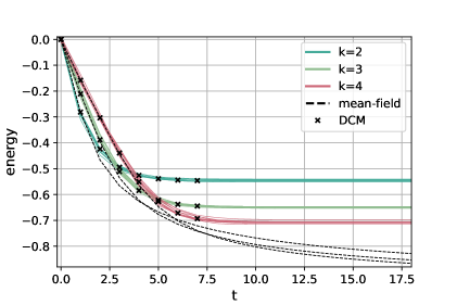
Even degree dynamics show fast convergence.
In the case of a hypergraph with an even degree, here , we observe in Fig. 3(a) that the energy quickly decreases during the first steps of the process, before it plateaus and converges to a value that depends on the order . Qualitatively similar results are found for higher (even) degrees . The convergence time for hypergraphs with degree grows logarithmically with the graph size , as numerically shown in Appendix C.1. For the mean-field approximation, however, the energy trajectory does not stop decreasing and approaches the stable fixed point as .
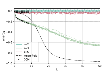
Mean field is accurate for odd degree dynamics with chaotic and slow convergence.
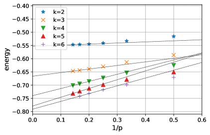
In the case , i.e. hypergraphs with an odd degree, only the settings give dynamical processes whose transient lengths are logarithmic in , as shown in Appendix C.1. For any other , the mean-field equations have a stable fixed point close to zero (between and ), and the numerical trajectories are observed to chaotically oscillate around the mean-field fixed point, see Fig. 9 in Appendix C.3. Their transient lengths grow exponentially with , as shown in Fig. 7 in Appendix C.3. Under those parameters, the dynamics are ineffective in reaching low-energy configurations. They adopt a chaotic behavior for an exponential time until they randomly visit a configuration belonging to an attractor. The qualitative behavior of their transient is correctly described by the mean-field equations, as can be seen in Fig. 3(b) and Fig. 9. However, Fig. 9 shows that the mean-field and DCM energies for odd values of approach two distinct, although very close, fixed points as grows. Because of the large transient length observed in this setting, the convergence of typical trajectories with cannot be studied either numerically or using the BDCM.
Special cases for odd degrees.
When , the trajectories do not stay stuck near the mean-field stable fixed point . Unlike , the energy keeps decreasing at a linear rate and plateaus slightly under . In Fig. 3(b), one observes that the DCM correctly ignores the mean field plateau. On the other hand, for , the dynamics get quickly trapped in cycles of length with energy close to zero. It was formally proven in [31] that quench dynamics on ordinary graphs, i.e. , always converge to limit cycles of length at most . On the other hand, large cycles () are numerically observed for . Given this qualitative difference, it would not be surprising to observe differences between the density of attractors around zero energy for and . This might explain why trajectories on -uniform hypergraphs quickly converge to limit cycles, whereas in the case the trajectories that get stuck at high energy need exponential time to find an attractor.
5.4 Attractors of the Process: Backtracking Dynamical Cavity Method
Recall that the BDCM allows us to count the attractors of size of the dynamics with an incoming path length . We can use this property to obtain information on the basin of attraction of a specific type of attractor. Here we focus on fixed points, as they represent stable solutions.
As we increase in our analysis, the entropy of the number of backtracking attractors that we find grows: We capture a larger fraction of the basin of attraction – i.e. the configurations that lead to these attractors within at most steps. Recall that we want to answer what energetic states the dynamics reaches. To do so, we compute observables to obtain properties of these attractors that are reached from the basin of attraction – here, we compute the energy of the fixed points.
Computing this value for would encompass the full basin of attraction. However, this is computationally unfeasible. Therefore we compute the observables for small and with some care we extrapolate to larger . Because of the limitations of analyzing only short trajectories, we focus only on processes that take to converge.
Energy in the attractor for even degree.
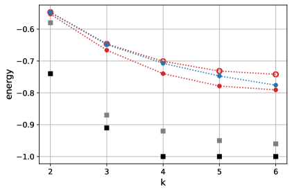
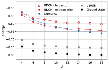
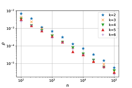
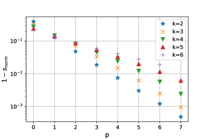
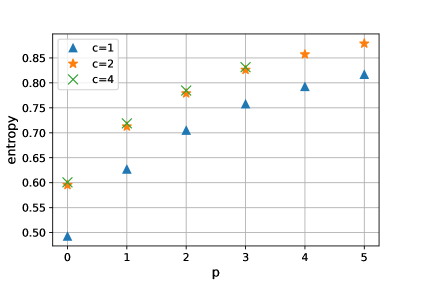
Fig. 4 shows evidence that the quench dynamics of -XOR-SAT instances with degree almost always end up in cycles of length , in the large limit. In Fig. 4(a), the fraction of rattlers of numerically observed attractors decreases as for . This empirical result aligns with the theoretical prediction in Fig. 4(b). Using (9) and the BDCM equations without Lagrange constraints ( and ), it shows that the normalized entropy of attractors with length approaches exponentially as the incoming path length increases. The BDCM predictions for attractors of length are exactly identical to those of length , indicating that in the large limit no attractor of length is reached from a non-negligible fraction of the initial configuration space. This result means that computing the energy of the attractor for the setting and growing values of gives the typical energy reached by a trajectory of this process on a -regular hypergraph. We approximate the energy in the limit by means of a linear fit of the values obtained from (11) with and evaluated at plotted as a function of . The value of the fit evaluated at then gives an approximation to the value of when is very large. Because of the computational complexity of the BDCM algorithm with large values, the approximation was computed from the results only. Its extrapolation over in Fig. 5 must therefore be taken with caution. As the connectivity of the hypergraph increases, only smaller values of are computationally tractable which makes the results for large or less precise. Fig. 5 shows that the extrapolated BDCM result for the energy is in reasonable agreement with the numerical simulations, extrapolated as .
In Fig. 5(a), we observe that the energy reached by the quench dynamics is very close to the 1dRSB phase transition for , whereas for they differ by . The 1dRSB phase transition corresponds to the energy under which the equilibrium properties of the system are described with replica symmetry breaking [35, 36, 37, 38]. Fig. 5(b) shows the energies for and increasing , rescaled to correspond to the fully connected -spin model [32, 33, 34] in the limit . The results suggest that the energy of the quench stays stuck well above the 1dRSB energy even in the large limit. This might indicate the emergence of a large number suboptimal frozen structures during the dynamical process in the case . For instance, if a well-connected subset of the hypergraph becomes static, i.e. enough hyperedges are satisfied for all node values belonging to them to be fixed, but a few hyperedges immersed in this frozen subset are unsatisfied, those unsatisfied hyperedges will be trapped until the end of the process. The number of such structures that can be found in random -XOR-SAT instances was studied in [39]. It was found that suboptimal structures exist with high probability in any instance of the XOR-SAT problem with .
Energy for odd degree – ().
We saw in Section 5.3 that hypergraphs with and numerically converge to cycles with close to zero energy, i.e. they essentially do not move away from the average energy of a random initial configuration. Recall that hypergraphs with are simple graphs as considered previously in [9]. In agreement with previous results, we recover that the normalized entropy associated with converges to as , whereas the result stays significantly lower than one, indicating that the dynamical process would converge almost always to -cycles. Consistent with the numerical observations, the energies obtained for are zero for all considered . Those results can be observed in Appendix C.3. It allows us to conclude that the quench dynamics in the system limit with parameters and almost always end in cycles of length and zero energy.
Energy for odd degree – ().
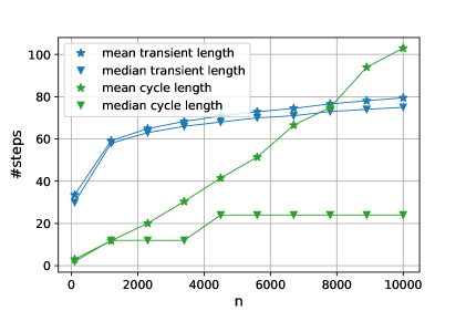
The case appears to be the only setting enabling hypergraphs of degree to reach low energy states with quench dynamics. However, one observes in Fig. 6(a) that the normalized entropy for small cycles does not quickly approach for growing values of the incoming path length . Furthermore, the entropy of each considered is strictly greater than the smaller lengths. Those observations indicate that, unlike the results seen for hypergraphs with even degrees, the trajectories do not end in small attractors . The BDCM does not allow the study of the basin of attraction of larger attractors, as evaluating the equations numerically becomes exponentially costly in . Fig. 6(b) shows the length of the cycles to which trajectories were numerically observed to converge and compares it to the transient length. Interestingly, for large enough , all observed cycle lengths were found to be multiples of , as presented in Fig. 10 in Appendix C.3. In Fig. 6(b) we see that, while both the mean and the median of the transient lengths grow logarithmically in the considered range of hypergraph size , the mean cycle length distances itself quickly from the median and becomes larger than the transient length. This suggests that the distribution of cycle lengths at large might be heavy-tailed.
6 Conclusion
In this work, we studied the quench dynamics of the XOR-SAT problem on -regular -uniform hypergraphs. A generalization of the BDCM introduced in [9] was developed to allow the study of dynamical processes on hypergraphs. Two versions of this extension were presented: a general version covering all synchronous, deterministic and locally defined update rules on hypergraphs, and a more specific one whose complexity depends linearly on the hyperedges size , instead of exponentially.
In our results we showed that the DCM is more effective than a naive mean field approach which failed to predict update rules with logarithmic convergence time, whereas the DCM successfully predicted the initial phase of the quench trajectories. The BDCM was used to determine the type of attractor to which typical trajectories converge, for different values of the degree and the order of the hypergraphs. In the case , it was found that almost all trajectories converge to fixed points. The BDCM enabled the evaluation of the performance of the quench dynamics to reach low-energy configurations. For the -XOR-SAT, it was observed that, as grows, the quench stays stuck above the energy at which the transition from RS to 1dRSB occurs. In the specific case , the dynamics were shown to converge in logarithmic time to large attractors, with plausibly a heavy-tailed distribution.
The generalization of the BDCM to hypergraphs opens many applications for studying dynamical properties of constraint satisfaction problems with interactions involving any number of variables. Examples of such problems involve the random K-SAT problem [40], the random bicoloring aka NAE-SAT problem [41], or the occupation problems studied in [42, 43]. This method provides a new perspective on the types of questions that can be addressed using the cavity method. However, further work would be needed to make the method applicable to stochastic processes, limiting the current applications to deterministic algorithms. The main limitation of the BDCM is its complexity growing exponentially with the length of the considered path.
Acknowledgments
This research was supported by the NCCR MARVEL, a National Center of Competence in Research, funded by the Swiss National Science Foundation (grant number 205602).
References
- [1] Fabrizio Altarelli, Rémi Monasson, Guilhem Semerjian, and Francesco Zamponi. A review of the statistical mechanics approach to random optimization problems. CoRR, abs/0802.1829, 2008.
- [2] M. Mézard and A. Montanari. Information, Physics, and Computation. Oxford Graduate Texts. OUP Oxford, 2009.
- [3] David Gamarnik. The overlap gap property: A topological barrier to optimizing over random structures. Proceedings of the National Academy of Sciences, 118(41), October 2021.
- [4] I. Neri and D. Bollé. The cavity approach to parallel dynamics of ising spins on a graph. Journal of Statistical Mechanics: Theory and Experiment, 2009(08):P08009, August 2009.
- [5] A. Y. Lokhov, M. Mézard, and L. Zdeborová. Dynamic message-passing equations for models with unidirectional dynamics. Physical Review E, 91(1), January 2015.
- [6] K. Mimura and A. C. C. Coolen. Parallel dynamics of disordered ising spin systems on finitely connected directed random graphs with arbitrary degree distributions. Journal of Physics A: Mathematical and Theoretical, 42(41):415001, September 2009.
- [7] Y. Kanoria and A. Montanari. Majority dynamics on trees and the dynamic cavity method. The Annals of Applied Probability, 21(5), October 2011.
- [8] J. P. L. Hatchett, B. Wemmenhove, I. P. Castillo, T. Nikoletopoulos, N. S. Skantzos, and A. C. C. Coolen. Parallel dynamics of disordered ising spin systems on finitely connected random graphs. Journal of Physics A: Mathematical and General, 37(24):6201–6220, June 2004.
- [9] F. Behrens, B. Hudcová, and L. Zdeborová. Backtracking dynamical cavity method. Physical Review X, 13(3), August 2023.
- [10] P. Carraresi, G. Gallo, and Gabriella Rago. A hypergraph model for constraint logic programming and applications to bus drivers’ scheduling. Annals of Mathematics and Artificial Intelligence, 8(3–4):247–270, September 1993.
- [11] A. Bretto. Applications of Hypergraph Theory: A Brief Overview, pages 111–116. Springer International Publishing, Heidelberg, 2013.
- [12] Nitin Ahuja and Anand Srivastav. On constrained hypergraph coloring and scheduling. In Klaus Jansen, Stefano Leonardi, and Vijay Vazirani, editors, Approximation Algorithms for Combinatorial Optimization, pages 14–25, Berlin, H., 2002. Springer Berlin Heidelberg.
- [13] J. van den Heuvel and M. Johnson. Transversals of subtree hypergraphs and the source location problem in digraphs. Networks, 51:113–119, 03 2008.
- [14] M. Ibrahimi, Y. Kanoria, M. Kraning, and A. Montanari. The set of solutions of random xorsat formulae. The Annals of Applied Probability, 25(5), October 2015.
- [15] M. Mezard, F. Ricci-Tersenghi, and R. Zecchina. Alternative solutions to diluted p-spin models and xorsat problems, 2002.
- [16] Simona Cocco, Rémi Monasson, Andrea Montanari, and Guilhem Semerjian. Approximate analysis of search algorithms with ”physical” methods. CoRR, cs.CC/0302003, 2003.
- [17] S. Franz, M. Mézard, F. Ricci-Tersenghi, M. Weigt, and R. Zecchina. A ferromagnet with a glass transition. Europhysics Letters (EPL), 55(4):465–471, August 2001.
- [18] F. Ricci-Tersenghi, M. Weigt, and R. Zecchina. Simplest randomk-satisfiability problem. Physical Review E, 63(2), January 2001.
- [19] Xiaoyu Xia and Peter G Wolynes. Fragilities of liquids predicted from the random first order transition theory of glasses. Proceedings of the National Academy of Sciences, 97(7):2990–2994, 2000.
- [20] Giulio Biroli and Jean-Philippe Bouchaud. The random first-order transition theory of glasses: a critical assessment. Structural Glasses and Supercooled Liquids: Theory, Experiment, and Applications, pages 31–113, 2012.
- [21] Freya Behrens, Barbora Hudcová, and Lenka Zdeborová. Dynamical phase transitions in graph cellular automata. Phys. Rev. E, 109:044312, Apr 2024.
- [22] B. Pittel and G. Sorkin. The satisfiability threshold for k-xorsat. Combinatorics, Probability and Computing, 25(2):236–268, 2016.
- [23] E. Gardner. Spin glasses with p-spin interactions. Nuclear Physics B, 257:747–765, 1985.
- [24] Sungmin Hwang, Viola Folli, Enrico Lanza, Giorgio Parisi, Giancarlo Ruocco, and Francesco Zamponi. On the number of limit cycles in asymmetric neural networks. Journal of Statistical Mechanics: Theory and Experiment, 2019(5):053402, may 2019.
- [25] L. Zdeborová and S. Boettcher. A conjecture on the maximum cut and bisection width in random regular graphs. Journal of Statistical Mechanics: Theory and Experiment, 2010(02):P02020, feb 2010.
- [26] L. Zdeborová and F. Krzakala. Generalization of the cavity method for adiabatic evolution of gibbs states. Physical Review B, 81(22), June 2010.
- [27] Marc Mézard and Giorgio Parisi. The bethe lattice spin glass revisited. The European Physical Journal B-Condensed Matter and Complex Systems, 20:217–233, 2001.
- [28] A. Y. Lokhov, M. Mézard, and L. Zdeborová. Dynamic message-passing equations for models with unidirectional dynamics. Physical Review E, 91(1), January 2015.
- [29] F. Behrens, G. Arpino, Y. Kivva, and L. Zdeborová. (dis)assortative partitions on random regular graphs. Journal of Physics A: Mathematical and Theoretical, 55(39):395004, September 2022.
- [30] G. Torrisi, R. Kühn, and A. Annibale. Uncovering the non-equilibrium stationary properties in sparse boolean networks. Journal of Statistical Mechanics: Theory and Experiment, 2022(5):053303, may 2022.
- [31] E. Goles-Chacc, F. Fogelman-Soulie, and D. Pellegrin. Decreasing energy functions as a tool for studying threshold networks. Discrete Applied Mathematics, 12(3):261–277, 1985.
- [32] P. Wang and R. Fazio. Dissipative phase transitions in the fully connected ising model with -spin interaction. Physical Review A, 103(1), January 2021.
- [33] B. Guiselin, L. Berthier, and G. Tarjus. Statistical mechanics of coupled supercooled liquids in finite dimensions. SciPost Physics, 12(3), March 2022.
- [34] A. Montanari and F. Ricci-Tersenghi. On the nature of the low-temperature phase in discontinuous mean-field spin glasses. The European Physical Journal B - Condensed Matter, 33(3):339–346, June 2003.
- [35] M. Mézard and G. Parisi. The bethe lattice spin glass revisited. The European Physical Journal B, 20(2):217–233, March 2001.
- [36] Marc Mezard and Andrea Montanari. Information, physics, and computation. Oxford University Press, 2009.
- [37] Marc Mézard and Giorgio Parisi. The cavity method at zero temperature. Journal of Statistical Physics, 111(1):1–34, 2003.
- [38] Cédric Koller, Freya Behrens, and Lenka Zdeborová. Counting and hardness-of-finding fixed points in cellular automata on random graphs. Journal of Physics A: Mathematical and Theoretical, 57(46):465001, November 2024.
- [39] S. Cocco, R. Monasson, A. Montanari, and G. Semerjian. Approximate analysis of search algorithms with ”physical” methods, 2003.
- [40] Marc Mézard, Giorgio Parisi, and Riccardo Zecchina. Analytic and algorithmic solution of random satisfiability problems. Science, 297(5582):812–815, 2002.
- [41] Amin Coja-Oghlan and Lenka Zdeborová. The condensation transition in random hypergraph 2-coloring. In Proceedings of the twenty-third annual ACM-SIAM symposium on Discrete Algorithms, pages 241–250. SIAM, 2012.
- [42] Lenka Zdeborová and Marc Mézard. Locked constraint satisfaction problems. Physical review letters, 101(7):078702, 2008.
- [43] Lenka Zdeborová and Marc Mézard. Constraint satisfaction problems with isolated solutions are hard. Journal of Statistical Mechanics: Theory and Experiment, 2008(12):P12004, 2008.
- [44] Florent Krzakała, Andrea Montanari, Federico Ricci-Tersenghi, Guilhem Semerjian, and Lenka Zdeborová. Gibbs states and the set of solutions of random constraint satisfaction problems. Proceedings of the National Academy of Sciences, 104(25):10318–10323, 2007.
Appendix A Mean Field Model
We introduce a mean field approximation as a competing method to the DCM for predicting the energy evolution at the start of the process. Starting from a random configuration of the system, where the node values are drawn independently from a Bernoulli distribution, the goal is to express the fraction of satisfied hyperedges at time in a recursive way. This enables us to iteratively compute the evolution of the energy of the system. The mean field approximation neglects the local correlations between neighboring hyperedges and thereby allows one to write the evolution of the hyperedge values as a function of the fraction of satisfied constraints only.
We start by writing a discrete Master equation for the probability of a hyperedge to be satisfied at time , i.e. . The difference in the probability of a hyperedge to be satisfied at time compared to the same probability at time can be decomposed: Into the probability that ( was unsatisfied) and then subsequently changed, minus the probability ( was satisfied) and subsequently changed. As a change in the value of the hyperedge at time is caused by an odd number of changes in the values of the nodes it contains at that very time, one can write:
| (50) | ||||
| (51) |
Following the mean-field approach, we assume the neighborhood of the nodes belonging to a hyperedge to be independent given the value of , i.e. all edges . Using this assumption, the probability of the number of nodes changing value between time and being odd can be expressed as:
| (52) |
Here, is the number of nodes belonging to the hyperedge and is a binomial random variable. It models a process with trials and a probability of success given by the probability of a node to change value between and given , which we assume to be independent as
| (53) |
for any . represents the number of nodes in that change value between and given .
This formulation enables us to model the probabilistic evolution of the hyperedge values as a function of the previous values only, getting rid of the individual node values . One can then consider the dual of the hypergraph where the hyperedge values become the nodes and the neighborhood of the nodes represent links between several hyperedges.
The key idea of the mean field approximation is to replace the interactions with individual elements of the system by the average of the interactions with the whole system. Applying this principle to the system of values, we replace the probability of a neighboring hyperedge to have a value by the fraction of hyperedges with value in the system , neglecting the dependency between the values of two neighboring edges. The for then become independent and identically distributed Bernouilli variables with probability . The probability of a node to flip at a given time step from (53) then becomes:
| (54) |
with a binomial random variable with parameters and . represents the number of satisfied hyperedges in the neighborhood of a node at time , excluding hyperedge , and takes all values such that the sum of the values of hyperedges in the neighborhood of is strictly smaller than zero.
Assuming the initial node values to be independent and identically distributed, is the same for all and can be denoted by . One notes that the update rule (50) is then identical for all and the evolution of the number of satisfied edges in the system can be modeled as:
| (55) | ||||
| (56) | ||||
| (57) |
| (58) |
The energy at a given timestep can then be obtained from as .
The mean field approximation is expected to produce very accurate results for the first few timesteps of the dynamical process, when neighboring hyperedge values have little correlation. As the system evolves, structures of hyperedge values can emerge, causing the energy to diverge from the mean-field prediction.
Appendix B 1-Step Replica Symmetry Breaking
| 1dRSB energy | -0.58 | -0.87 | -0.92 | -0.95 | -0.96 |
|---|
Equations (44)-(49) are written under the Replica Symmetric (RS) assumption [36]. In the RS phase, almost all trajectories with non-zero measure (5) belong to the same pure state. A pure state is defined by a solution to the BP equations. However, this assumption does not hold in general for the low-temperature phase of disordered systems [36]. The phase transition from RS to the so-called Dynamic 1-step Replica Symmetry Breaking (d1RSB) is usually associated with a transition towards a phase that is hard to sample uniformly [44]. The d1RSB phase is characterized by the existence of exponentially many pure states (w.r.t. the system’s size ) among which the free entropy density is split.
In this section, we describe the equations and algorithm used to find the energy at which the phase transition from RS to d1RSB occurs for the -XOR-SAT model. To this end, we set and , which brings us back to the usual cavity method where the probability distribution (5) is written over configurations instead of trajectories .
We define a probability measure over the pure states as
| (59) |
where is the free entropy density of the pure state defined by the solution . The replicated free entropy density is then given by
| (60) |
The replicated free entropy density can be estimated by defining an auxiliary graphical model and applying the BP procedure. This approach was first introduced in [35]. Detailed explanations about how to write the BP equations of the auxiliary model can be found in [35, 36, 37]. This results in the following system of self-consistent equations:
| (61) | ||||
| (62) |
| (63) | ||||
| (64) | ||||
| (65) | ||||
| (66) |
The phase transition from RS to d1RSB occurs at the point from which the results given by the 1RSB equations (61)-(66) diverge from the equations written under the RS assumption, (44)-(44). Solving the d1RSB equations can be done by means of a population dynamics algorithm explained in [35, 38]. The results for the energy at which the d1RSB phase transition occurs for the -XOR-SAT with degree are shown in Table 2, and compared in Fig. 5(a) with the energies reached by the quench dynamics.
Appendix C Additional Results
C.1 Transient lengths
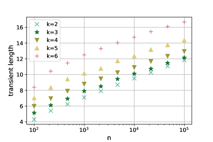
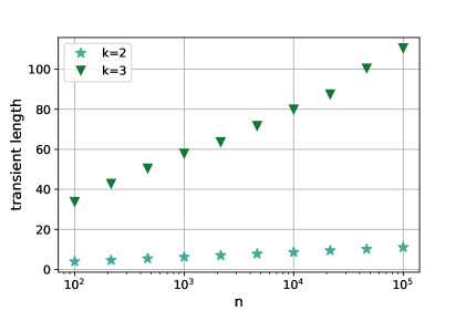
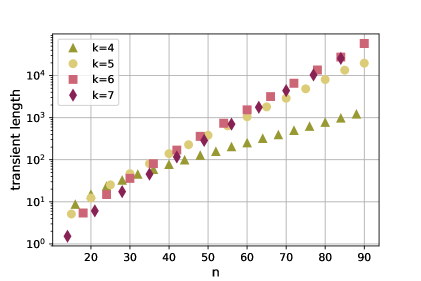
The average transient length of trajectories are shown in Fig. 7(a) for hypergraphs with degree , and Fig. 7(b) and 7(c) for hypergraphs with , and different values of the order . In the case , the transient length grows logarithmically with the size of the hypergraph , for all considered values of . The plot indicates that all values have a similar slope. However, the offset difference between them increases with . For on the other hand, only are observed to have a logarithmic growth. While the slope of is of the same order as the case, grows at a significantly greater rate. For the other observed values , the transient lengths are proportional to the exponential of . This makes the dynamics on -regular hypergraphs with order very computationally costly to simulate for large values of or to analyze with methods whose complexities grow exponentially with the length of the considered paths, such as the BDCM.
C.2 Even degree
| 2 | 3 | 4 | 5 | 6 | ||||||
|---|---|---|---|---|---|---|---|---|---|---|
| energy | entropy | energy | entropy | energy | entropy | energy | entropy | energy | entropy | |
| 0 | -0.362 | 0.603 | -0.417 | 0.677 | -0.458 | 0.724 | -0.489 | 0.758 | -0.514 | 0.783 |
| 1 | -0.476 | 0.868 | -0.538 | 0.851 | -0.577 | 0.853 | -0.603 | 0.859 | -0.623 | 0.866 |
| 2 | -0.516 | 0.952 | -0.586 | 0.928 | -0.625 | 0.918 | -0.651 | 0.914 | -0.671 | 0.912 |
| 3 | -0.533 | 0.981 | -0.613 | 0.967 | -0.653 | 0.955 | -0.679 | 0.946 | -0.698 | 0.940 |
| 4 | -0.541 | 0.992 | -0.629 | 0.985 | -0.672 | 0.976 | -0.698 | 0.967 | -0.717 | 0.959 |
| 5 | -0.545 | 0.997 | -0.639 | 0.994 | -0.686 | 0.988 | -0.713 | 0.980 | -0.731 | 0.972 |
| 6 | -0.546 | 0.999 | -0.644 | 0.998 | -0.695 | 0.994 | -0.723 | 0.989 | -0.742 | 0.981 |
| 7 | -0.547 | 0.9995 | -0.647 | 0.999 | -0.701 | 0.998 | -0.732 | 0.994 | - | - |
| p | 0 | 1 | 2 | 3 | 4 | 5 | 6 | 7 | ||||||||
|---|---|---|---|---|---|---|---|---|---|---|---|---|---|---|---|---|
| energy | entropy | energy | entropy | energy | entropy | energy | entropy | energy | entropy | energy | entropy | energy | entropy | energy | entropy | |
| d | ||||||||||||||||
| 4 | -0.417 | 0.677 | -0.538 | 0.851 | -0.586 | 0.928 | -0.613 | 0.967 | -0.629 | 0.985 | -0.639 | 0.994 | -0.644 | 0.998 | -0.647 | 0.999 |
| 6 | -0.361 | 0.637 | -0.464 | 0.807 | -0.506 | 0.890 | -0.530 | 0.936 | -0.544 | 0.963 | -0.555 | 0.979 | -0.562 | 0.989 | - | - |
| 8 | -0.324 | 0.612 | -0.415 | 0.778 | -0.453 | 0.863 | -0.474 | 0.913 | -0.487 | 0.944 | -0.497 | 0.964 | - | - | - | - |
| 10 | -0.297 | 0.594 | -0.379 | 0.758 | -0.414 | 0.844 | -0.433 | 0.896 | -0.446 | 0.929 | -0.454 | 0.951 | - | - | - | - |
| 12 | -0.276 | 0.581 | -0.352 | 0.742 | -0.384 | 0.829 | -0.402 | 0.882 | -0.413 | 0.916 | -0.421 | 0.940 | - | - | - | - |
| 14 | -0.259 | 0.570 | -0.330 | 0.730 | -0.360 | 0.817 | -0.377 | 0.870 | -0.388 | 0.905 | - | - | - | - | - | - |
| 16 | -0.245 | 0.561 | -0.312 | 0.720 | -0.340 | 0.806 | -0.356 | 0.860 | -0.366 | 0.896 | - | - | - | - | - | - |
| 18 | -0.233 | 0.554 | -0.318 | 0.535 | -0.324 | 0.798 | -0.339 | 0.852 | -0.348 | 0.889 | - | - | - | - | - | - |
| 20 | -0.223 | 0.548 | -0.283 | 0.705 | -0.309 | 0.791 | -0.323 | 0.845 | - | - | - | - | - | - | - | - |
| 22 | -0.214 | 0.542 | -0.271 | 0.698 | -0.296 | 0.784 | -0.310 | 0.839 | - | - | - | - | - | - | - | - |
Table 3 contains all BDCM results for the entropy and energy of backtracking attractors with incoming path length on -regular hypergraphs with order , and -uniform hypergraphs with even degree values in . They are obtained using (9) and (11) respectively after convergence of the BP messages (44) and (45).
The results for the energy are then used in Fig. 8(b) to obtain an approximation of the energy in the attractor of a typical trajectory. The last points for each are linearly fitted and extrapolated at . The same procedure is applied in Fig. 8(a) to obtain the extrapolation of the numerical results for the energies in the limit . Those values are used in Fig. 5(a) and compared with the ground state energies of the system and the energies under which the replica symmetric ansatz does not hold anymore.
C.3 Odd degree
| k | 5 | 7 | ||
|---|---|---|---|---|
| DCM | mean field | DCM | mean field | |
| p | ||||
| 0 | 0.000000 | 0.000000 | 0.000000 | 0.000000 |
| 1 | -0.031250 | -0.031250 | -0.007812 | -0.007812 |
| 2 | -0.032473 | -0.032624 | -0.007853 | -0.007856 |
| 3 | -0.032694 | -0.032747 | -0.007853 | -0.007856 |
| 4 | -0.032724 | -0.032758 | -0.007853 | -0.007856 |
| 5 | -0.032728 | -0.032759 | -0.007853 | -0.007856 |
| 6 | -0.032729 | -0.032759 | -0.007853 | -0.007856 |
Evolution of the energy for
Fig. 9 shows the numerical evolution of the energy for the quench dynamics on -regular hypergraphs with and compares it to the mean field prediction. For each , the mean-field equations have a stable fixed point between and . The mean field energies initialized with are observed to quickly approach their respective stable fixed points. We see that the averages of the numerical energies closely follow the mean-field predictions. The numerical trajectories chaotically oscillate around the mean-field fixed points and are unable to reach low energies.
Cycle lengths for and are multiples of
In Fig. 10, we see that the fraction of trajectories that does not end up in an attractor whose length is a multiple of decreases at an exponential rate as the hypergraph size increases. This indicates that in the large system limit, almost all trajectories ruled by this process eventually converge to cycles with length for some random variable whose (unknown) distribution depends on the hypergraph size .
Table 4 contains the BDCM results for the entropy and energy of backtracking attractors with incoming path length on -regular hypergraphs with order . The entropy and energy are computed for different cycle lengths and all values of for which the BDCM algorithm is computationally tractable. The entropy results for are plotted in Fig. 6(a).
| 2 | 3 | ||||
| energy | entropy | energy | entropy | ||
| 1 | 0 | -0.600 | 0.339 | -0.660 | 0.493 |
| 1 | -0.688 | 0.587 | -0.745 | 0.627 | |
| 2 | -0.724 | 0.676 | -0.770 | 0.705 | |
| 3 | -0.745 | 0.709 | -0.781 | 0.757 | |
| 4 | -0.758 | 0.725 | -0.801 | 0.792 | |
| 5 | -0.766 | 0.732 | -0.815 | 0.817 | |
| 2 | 0 | 0.000 | 0.678 | -0.500 | 0.595 |
| 1 | 0.000 | 0.903 | -0.563 | 0.713 | |
| 2 | 0.000 | 0.969 | -0.598 | 0.779 | |
| 3 | 0.000 | 0.988 | -0.611 | 0.826 | |
| 4 | 0.000 | 0.996 | -0.627 | 0.857 | |
| 5 | 0.000 | 0.998 | -0.639 | 0.879 | |
| 4 | 0 | 0.000 | 0.678 | -0.494 | 0.601 |
| 1 | 0.000 | 0.903 | -0.552 | 0.719 | |
| 2 | 0.000 | 0.969 | -0.586 | 0.785 | |
| 3 | 0.000 | 0.988 | -0.598 | 0.831 | |