Numerical evaluation of two-loop QCD helicity amplitudes for $gg\to t{\bar{t}}g$ at leading colour

Abstract

We present the first benchmark evaluation of the two-loop finite remainders for the production of a top-quark pair in association with a jet at hadron colliders in the gluon channel. We work in the leading colour approximation, and perform the numerical evaluation in the physical phase space. To achieve this result, we develop a new method for expressing the master integrals in terms of a (over-complete) basis of special functions that enables the infrared and ultraviolet poles to be cancelled analytically despite the presence of elliptic Feynman integrals. The special function basis makes it manifest that the elliptic functions appear solely in the finite remainder, and can be evaluated numerically through generalised series expansions. The helicity amplitudes are constructed using four dimensional projectors combined with finite-field techniques to perform integration-by-parts reduction, mapping to special functions and Laurent expansion in the dimensional regularisation parameter.

1 Introduction

The production of a top-quark pair in association with a jet is a high priority process for precision studies at the Large Hadron Collider (LHC), particularly at its high-luminosity phase (HL-LHC). The sensitivity to fundamental parameters of the Standard Model and the increasing precision of experimental data demand that this process is computed to at least next-to-next-to-leading order (NNLO) accuracy in QCD, for which theoretical challenges must be overcome.

A significant fraction (around 50%) of all $t\bar{t}$ signals at the LHC are associated with an additional QCD jet and have been extensively studied by the ATLAS and CMS experiments CMS:2016oae ; ATLAS:2018acq ; CMS:2020grm ; CMS:2024ybg . Normalised distributions for this event are highly sensitive to the top quark mass and extensive studies have been made to develop a competitive parameter-extraction procedure Alioli:2013mxa ; Bevilacqua:2017ipv ; Alioli:2022ttk ; Alioli:2022lqo . Next-to-leading order (NLO) theory predictions have been available for nearly 20 years Dittmaier:2007wz and are now simple to compute using modern automated tools such as OpenLoops2 Buccioni:2019sur , Helac-NLOBevilacqua:2011xh or MadGraph5_aMC@NLO Alwall:2014hca . The theory-level input to such studies is currently at the level of NLO in QCD matched to a parton shower (NLO+PS), which has been implemented within the Powheg-Box framework Alioli:2011as with complete off-shell effects also available at fixed order Bevilacqua:2015qha ; Bevilacqua:2016jfk . Furthermore, mixed QCD and electroweak (EW) corrections have also been calculated G_tschow_2018 . Extending theoretical predictions to NNLO QCD accuracy presents a major challenge since one must overcome bottlenecks associated with the large number of variables of a three-particle final state and the analytic complexity of the Feynman integrals with internal masses. Such difficulties mean that the two-loop amplitudes entering the double virtual corrections to the cross section are still currently unknown. The use of finite field reconstruction techniques vonManteuffel:2014ixa ; Peraro:2016wsq ; Klappert:2019emp ; Peraro:2019svx ; Smirnov:2019qkx ; Klappert:2020aqs ; Klappert:2020nbg has had a dramatic effect on our ability to evaluate the double virtual corrections to complicated $2\to 3$ scattering processes with massless internal particles Badger:2019djh ; Badger:2021nhg ; Badger:2021ega ; Abreu:2021asb ; Badger:2022ncb ; Agarwal:2021vdh ; Badger:2021imn ; Abreu:2023bdp ; Badger:2023mgf ; Agarwal:2023suw ; DeLaurentis:2023nss ; DeLaurentis:2023izi , with up to one additional external scale Badger:2021nhg ; Badger:2021ega ; Abreu:2021asb ; Badger:2022ncb ; Badger:2024sqv ; Badger:2024awe and including internal massive propagators Agarwal:2024jyq . Progress has also required the development of highly optimised integration-by-parts reduction techniques Gluza:2010ws ; Ita:2015tya ; Larsen:2015ped ; Wu:2023upw and improved analytic understanding of multi-scale Feynman integrals through their differential equations Gehrmann:2015bfy ; Papadopoulos:2015jft ; Abreu:2018rcw ; Chicherin:2018mue ; Chicherin:2018old ; Abreu:2018aqd ; Abreu:2020jxa ; Canko:2020ylt ; Abreu:2021smk ; Kardos:2022tpo ; Abreu:2023rco leading to numerically efficient bases of special functions referred to as pentagon functions Gehrmann:2018yef ; Chicherin:2020oor ; Chicherin:2021dyp ; Abreu:2023rco ; Gehrmann:2024tds ; FebresCordero:2023pww . The new results have been combined with unresolved radiation contributions to provide differential distributions at NNLO QCD for a variety of important experimental measurements Chawdhry:2019bji ; Kallweit:2020gcp ; Chawdhry:2021hkp ; Czakon:2021mjy ; Badger:2021ohm ; Chen:2022ktf ; Alvarez:2023fhi ; Badger:2023mgf ; Hartanto:2022qhh ; Hartanto:2022ypo ; Buonocore:2022pqq ; Catani:2022mfv ; Buonocore:2023ljm ; Mazzitelli:2024ura ; Devoto:2024nhl ; Biello:2024pgo .

In this article we continue the efforts to compute the double virtual corrections at NNLO. To this point, the corrections at one-loop order expanded to $\mathcal{O}(\epsilon^{2})$ have been considered Badger:2022mrb and the differential equations (DEs) for the two-loop master integrals in the leading colour limit have been recently completed Badger:2022hno ; Badger:2024fgb . A major difference compared to other amplitudes with $2\to 3$ kinematics that have been previously studied is the presence of elliptic functions in the master integrals Bourjaily:2022bwx . This feature makes the computation more challenging than in the previous cases. In scenarios where all propagators are massless, the DEs were cast in a canonical form Henn:2013pwa , where the dimensional regulator factorises and the connection matrix contains solely logarithmic one-forms (‘dlogs’). This form of the DEs could then be solved in terms of a basis of polylogarithmic special functions known as pentagon functions Gehrmann:2018yef ; Chicherin:2020oor ; Badger:2021nhg ; Chicherin:2021dyp ; Abreu:2023rco . The latter are algebraically independent—in this sense they are a ‘basis’—and thus give a unique representation of the amplitudes where cancellations and simplifications are manifest. Furthermore, they are both fast and stable for numerical evaluation. Both of these advantages are spoiled by the presence of elliptic functions. First, the fact that we do not have a canonical form of the DEs means that we cannot write the solution in terms of a basis of special functions. This is a problem because the algebraic complexity of the amplitude at the level of the master integral is significantly greater than after the expansion in the dimensional regulator and resolution of the functional relations. Second, the numerical evaluation of the master integrals in this case is substantially less efficient than in the fully canonical scenario Badger:2024fgb .

To address these challenges, we propose a strategy aimed at minimising the impact of the non-polylogarithmic functions. We solve the non-canonical DEs for the master integrals in terms of a set of special functions that is potentially over-complete, but that nonetheless allows us to subtract analytically the ultraviolet (UV) and infrared (IR) poles of the two-loop amplitudes, and unlocks important simplifications in the latter. The large majority of the special functions are polylogarithmic and are thus suitable to be evaluated with the method applied to the pentagon functions. For the few non-polylogarithmic functions, we set up a minimal system of DEs which we solve by means of generalised power series Moriello:2019yhu ; Hidding:2020ytt .

We employ this special-function representation of the master integrals in the computation the two-loop leading-colour amplitude for the production of two on-shell top quarks and a gluon in the gluon-fusion channel ($gg\to t\bar{t}g$) without closed fermion loops. From the amplitude point of view, this is the most complicated partonic channel contributing to $t\bar{t}$ production in association with a jet at hadron colliders. Obtaining analytic expressions for this amplitude is a huge challenge on its own due to the high algebraic complexity of the rational functions accompanying the master integrals or special functions. We set up a routine based on finite-field arithmetic to evaluate numerically the two-loop amplitude, while concurrently also assess different strategies to derive its analytic form. We employ the four-dimensional projection method Peraro:2019cjj ; Peraro:2020sfm ; Buccioni:2023okz to derive the helicity amplitudes and present benchmark numerical evaluations in physical kinematics.

Our paper is organised as follows: We begin in section˜2 by outlining the structure of the leading colour amplitude, its pole structure and definition of the finite remainder. In section˜3 we describe the application of the four dimensional projector method to compute helicity amplitudes suitable for the description of top-quark decays in the narrow width approximation. In section˜4 we discuss the basis of functions used to describe the finite remainder before presenting benchmark evaluations and cross-checks in section˜5. We conclude with a summary and remarks regarding the prospects for the derivation of amplitudes suitable for phenomenological applications.

2 Colour and pole structure of the leading colour amplitude

We consider the partonic process

$$g(-p_{4})+g(-p_{5})\to\bar{t}(p_{1})+t(p_{2})+g(p_{3})\,.$$ (1)

We work in the ’t Hooft-Veltman (HV) scheme with $d=4-2\epsilon$ space-time dimensions and four-dimensional external momenta $p_{i}$. The latter are all outgoing and satisfy the following momentum-conservation and on-shell conditions,

$$p_{1}+p_{2}+p_{3}+p_{4}+p_{5}=0\,,\qquad\quad p_{1}^{2}=p_{2}^{2}=m_{t}^{2},\qquad\quad p_{3}^{2}=p_{4}^{2}=p_{5}^{2}=0\,,$$ (2)

where $m_{t}$ is the top-quark mass. The kinematics are described by six scalar invariants, which we choose as

$$\vec{d}=\bigl{(}d_{12},d_{23},d_{34},d_{45},d_{15},m_{t}^{2}\bigr{)}\,,$$ (3)

with $d_{ij}=p_{i}\cdot p_{j}$, and one pseudo-scalar invariant,

$$\mathrm{tr}_{5}=4\,\mathrm{i}\,\varepsilon_{\mu\nu\rho\sigma}\,p_{1}^{\mu}p_{2}^{\nu}p_{3}^{\rho}p_{4}^{\sigma}\,,$$ (4)

where $\varepsilon_{\mu\nu\rho\sigma}$ is the anti-symmetric Levi-Civita pseudo-tensor.

We compute the two-loop amplitude in the limit of a large number of colours $N_{c}$, neglecting the contributions from closed fermion loops. Only planar diagrams contribute at the leading order in this limit, resulting in a simpler set of Feynman integrals. The leading colour $L$-loop bare amplitude $\mathcal{A}^{(L)}_{\rm LC}$ has the following colour decomposition in terms of partial amplitudes $A^{(L)}$,

$$\begin{aligned} \mathcal{A}^{(L)}_{\rm LC}\big{(}1_{\bar{t}},\,&2_{t},3_{g},4_{g},5_{g}\big{)}=\sqrt{2}\;\overline{g}_{s}^{3}\,n^{L}\sum_{\sigma\in Z_{3}}\left(t^{a_{\sigma(3)}}t^{a_{\sigma(4)}}t^{a_{\sigma(5)}}\right)^{\bar{i}_{1}}_{\ i_{2}}A^{(L)}\bigl{(}1_{\bar{t}},\,2_{t},\sigma(3)_{g},\sigma(4)_{g},\sigma(5)_{g}\bigr{)}\,,\end{aligned}$$ (5)

where $\overline{g}_{s}$ is the bare strong coupling constant, $n=N_{c}(4\pi)^{\epsilon}\mathrm{e}^{-\epsilon\gamma_{E}}\overline{\alpha}_{s}/(4\pi)$, $\overline{\alpha}_{s}=\overline{g}_{s}^{2}/(4\pi)$, $Z_{3}$ is the set of cyclic permutations of $(3,4,5)$, $t^{a_{i}}$ are the fundamental generators of the $SU(N_{c})$ group normalised according to $\mathrm{tr}(t^{a}t^{b})=\delta^{ab}/2$, $a_{i}=1,\dots,8$ index the adjoint representation, and $i_{2}\,(\bar{i}_{1})=1,2,3$ index the fundamental (anti-fundamental) representation.

We define gauge invariant one- and two-loop partial amplitudes by including the additive renormalisation of the top-quark mass, as

$$\begin{aligned} A^{(1)}_{\mathrm{mren}}&=A^{(1)}-\delta Z_{m}^{(1)}A^{(0)}_{\mathrm{mct}}\,,\\ A^{(2)}_{\mathrm{mren}}&=A^{(2)}-\delta Z_{m}^{(2)}A^{(0)}_{\mathrm{mct}}+(\delta Z_{m}^{(1)})^{2}A^{(0)}_{2\mathrm{mct}}-\delta Z_{m}^{(1)}A^{(1)}_{\mathrm{mct}}\,.\end{aligned}$$ (6)

Here, $A^{(0)}_{\mathrm{mct}}$ is the tree-level amplitude with the insertion of a single mass counterterm in the internal massive propagator, $A^{(0)}_{2\mathrm{mct}}$ is the tree-level amplitude with two mass-counterterm insertions, and $A^{(1)}_{\mathrm{mct}}$ is the one-loop amplitude with one mass-counterterm insertion. Examples of diagrams contributing to $A^{(0)}_{\mathrm{mct}}$, $A^{(0)}_{2\mathrm{mct}}$ and $A^{(1)}_{\mathrm{mct}}$ are shown in fig.˜1. Moreover, in eq.˜6, $\delta Z_{m}^{(L)}$ denotes the $L$-loop top-quark mass-renormalisation factors, for which a representation in terms of Feynman integrals was provided in Ref. Badger:2021owl . This form of the mass counterterms allows us to check the gauge invariance of the amplitudes already at the level of the master integrals. For completeness, we provide the expression of all renormalisation factors in appendix˜A.

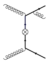
(a) $A^{(0)}_{\mathrm{mct}}$

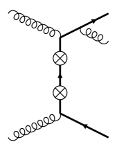
(b) $A^{(0)}_{2\mathrm{mct}}$

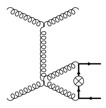
(c) $A^{(1)}_{\mathrm{mct}}$

Figure 1: Examples of Feynman diagrams with one and two mass-counterterm insertions, together with the terms of eq.˜6 they contribute to. Thick lines denote massive particles, and crossed circles indicate the counterterm insertions.

In order to subtract the remaining UV singularities, we renormalise also the top-quark wavefunction and the strong coupling constant ${\alpha_{s}}$. The counterterm associated with the gluon wavefunction contributes only to the amplitude terms arising from closed loops of heavy quarks Mitov:2006xs ; Czakon:2007wk , which are excluded from our leading colour computation. The renormalised partial amplitudes read

$$\begin{aligned} A^{(1)}_{\mathrm{ren}}=\ &A^{(1)}_{\mathrm{mren}}+\left(\frac{3}{2}\delta Z_{{\alpha_{s}}}^{(1)}+\delta Z_{t}^{(1)}\right)A^{(0)}\,,\\ A^{(2)}_{\mathrm{ren}}=\ &A^{(2)}_{\mathrm{mren}}+\left(\frac{5}{2}\delta Z_{{\alpha_{s}}}^{(1)}+\delta Z_{t}^{(1)}\right)A^{(1)}_{\mathrm{mren}}\\ &+\left(\frac{3}{2}\delta Z_{{\alpha_{s}}}^{(2)}+\frac{5}{2}\delta Z_{{\alpha_{s}}}^{(1)}\delta Z_{t}^{(1)}+\delta Z_{t}^{(2)}+\frac{3}{8}(\delta Z_{{\alpha_{s}}}^{(1)})^{2}\right)A^{(0)}\,,\end{aligned}$$ (7)

where the superscripts refer to the order in the renormalised strong coupling constant ${\alpha_{s}}$. Moreover, $A^{(1)}_{\mathrm{mren}}$ is the mass-renormalised one-loop amplitude defined in (6) and $A^{(0)}$ is the tree-level amplitude. The $L$-loop renormalisation constants $\delta Z^{(L)}_{t}$ Melnikov:2000zc and $\delta Z^{(L)}_{{\alpha_{s}}}$ are given in appendix˜A.

The renormalised partial amplitudes still contain divergences of IR nature. The pole structure of these divergences can be predicted by universal formulae describing the IR behaviour of QCD amplitudes CATANI1998161 ; Becher:2009cu ; Becher_2009 ; Gardi:2009qi ; Gardi:2009zv ; Catani:2000ef ; Ferroglia:2009ep ; Ferroglia:2009ii . We define the partial finite remainders as

$$\begin{aligned} R^{(0)}&=A^{(0)}\,,\\ R^{(1)}&=A^{(1)}_{\mathrm{ren}}-\mathbf{Z}^{(1)}A^{(0)}\,,\\ R^{(2)}&=A^{(2)}_{\mathrm{ren}}-\left(\mathbf{Z}^{(2)}-(\mathbf{Z}^{(1)})^{2}\right)A^{(0)}-\mathbf{Z}^{(1)}A^{(1)}_{\mathrm{ren}}\,.\end{aligned}$$ (8)

The relation between the partial finite remainders $R^{(L)}$ and the colour-dressed finite remainder $\mathcal{R}^{(L)}$ at leading colour takes the same form as for the bare amplitude, shown in eq.˜5, upon replacing $\mathcal{A}\rightarrow\mathcal{R}$ and $A\rightarrow R$. The expression of the IR pole operators $\mathbf{Z}^{(L)}$ are given in appendix˜A.

3 Helicity amplitudes for $gg\to t\bar{t}g$ scattering

In this section we discuss the construction of the helicity amplitudes for $gg\to t\bar{t}g$ and our computational framework. We adopt the massive spinor helicity formalism of Ref. Kleiss:1985yh , where each massive momentum $p$ ($p^{2}=m^{2}$) is first decomposed into two massless ones, as

$$p^{\mu}=p^{\flat,\mu}+\frac{m^{2}}{2\,p^{\flat}\cdot n}\,n^{\mu}\,,$$ (9)

where $(p^{\flat})^{2}=0$ and $n^{2}=0$. Massive spinors are then be constructed from the massless reference vector $n$ via

$$\bar{u}_{+}(p,m)=\frac{\langle n|(\not{p}+m)}{\langle np^{\flat}\rangle},\qquad\qquad v_{+}(p,m)=\frac{(\not{p}-m)|n\rangle}{\langle p^{\flat}n\rangle}\,.$$ (10)

We only need to consider the $+$ helicity configuration, since the $-$ one can be obtained from the latter by exchanging the two massless momenta $p^{\flat}$ and $n$,

$$\bar{u}_{-}(p,m)=\frac{\langle p^{\flat}n\rangle}{m}\bigg{(}\bar{u}_{+}(p,m)\bigg{|}_{p^{\flat}\leftrightarrow n}\bigg{)}\,.$$ (11)

We refer to Ref. Badger:2021owl for further details on this formalism.

In order to derive helicity amplitudes which depend on arbitrary reference momenta for the top and anti-top quarks ($n_{1}$ and $n_{2}$, respectively), we perform a decomposition using a basis made out of the $n_{1}$ and $n_{2}$ spinors Badger:2021owl ; Badger:2022mrb :

$$\begin{aligned} A^{(L)}(1^{+}_{\bar{t}},2^{+}_{t},3^{h_{3}}_{g},4^{h_{4}}_{g},5^{h_{5}}_{g};n_{1},n_{2})&=\frac{m_{t}\,\Phi^{h_{3}h_{4}h_{5}}}{\langle 1^{\flat}n_{1}\rangle\langle 2^{\flat}n_{2}\rangle}\bigg{\{}\langle n_{1}n_{2}\rangle s_{34}\;A^{(L),[1]}(1^{+}_{\bar{t}},2^{+}_{t},3^{h_{3}}_{g},4^{h_{4}}_{g},5^{h_{5}}_{g})\\ &\qquad+\langle n_{1}3\rangle\langle n_{2}4\rangle[34]\;A^{(L),[2]}(1^{+}_{\bar{t}},2^{+}_{t},3^{h_{3}}_{g},4^{h_{4}}_{g},5^{h_{5}}_{g})\\ &\qquad+\langle n_{1}3\rangle\langle n_{2}3\rangle\frac{[3|4|5|3]}{s_{34}}\;A^{(L),[3]}(1^{+}_{\bar{t}},2^{+}_{t},3^{h_{3}}_{g},4^{h_{4}}_{g},5^{h_{5}}_{g})\\ &\qquad+\langle n_{1}4\rangle\langle n_{2}4\rangle\frac{[4|5|3|4]}{s_{34}}\;A^{(L),[4]}(1^{+}_{\bar{t}},2^{+}_{t},3^{h_{3}}_{g},4^{h_{4}}_{g},5^{h_{5}}_{g})\bigg{\}}\,,\end{aligned}$$ (12)

where $s_{ij}=(p_{i}+p_{j})^{2}$. The decomposition above applies to the $L$-loop bare, mass-renormalised and renormalised partial amplitudes ($A^{(L)}$, $A^{(L)}_{\mathrm{mren}}$ and $A^{(L)}_{\rm ren}$), as well as to the partial finite remainders ($R^{(L)}$). The prefactors appearing in the ($n_{1}$,$n_{2}$) decomposition are chosen in such a way that the sub-amplitudes $A^{(L),[i]}$ are free of spinor phases and dimensionless. We choose the helicity-dependent gluonic phase factors for the three independent gluon helicity configurations: ($+++$, $++-$, $+-+$) as

$$\Phi^{+++}=\frac{[35]}{\langle 34\rangle\langle 45\rangle}\,,\qquad\quad\Phi^{++-}=\frac{\langle 5|3|4|5\rangle}{\langle 34\rangle^{2}}\,,\qquad\quad\Phi^{+-+}=\frac{\langle 4|5|3|4\rangle}{\langle 35\rangle^{2}}\,.\qquad\quad$$ (13)

We then evaluate the helicity amplitude at 4 different values of the ($n_{1}$,$n_{2}$) pair to obtain the sub-amplitudes $A^{(L),[i]}$ by inverting the following system of equations,

$$\begin{aligned} A^{(L)}(1^{+}_{\bar{t}},2^{+}_{t},3^{h_{3}}_{g},4^{h_{4}}_{g},5^{h_{5}}_{g};p_{3},p_{3})&=\frac{m_{t}\Phi^{h_{3}h_{4}h_{5}}}{\langle 1^{\flat}3\rangle\langle 2^{\flat}3\rangle}\langle 34\rangle^{2}\frac{[4|5|3|4]}{s_{34}}\;A^{(L),[4]}(1^{+}_{\bar{t}},2^{+}_{t},3^{h_{3}}_{g},4^{h_{4}}_{g},5^{h_{5}}_{g})\,,\\ A^{(L)}(1^{+}_{\bar{t}},2^{+}_{t},3^{h_{3}}_{g},4^{h_{4}}_{g},5^{h_{5}}_{g};p_{3},p_{4})&=\frac{m_{t}\Phi^{h_{3}h_{4}h_{5}}}{\langle 1^{\flat}3\rangle\langle 2^{\flat}4\rangle}\langle 34\rangle s_{34}\;A^{(L),[1]}(1^{+}_{\bar{t}},2^{+}_{t},3^{h_{3}}_{g},4^{h_{4}}_{g},5^{h_{5}}_{g})\,,\\ A^{(L)}(1^{+}_{\bar{t}},2^{+}_{t},3^{h_{3}}_{g},4^{h_{4}}_{g},5^{h_{5}}_{g};p_{4},p_{3})&=-\frac{m_{t}\Phi^{h_{3}h_{4}h_{5}}}{\langle 1^{\flat}4\rangle\langle 2^{\flat}3\rangle}\bigg{[}\langle 34\rangle s_{34}\;A^{(L),[1]}(1^{+}_{\bar{t}},2^{+}_{t},3^{h_{3}}_{g},4^{h_{4}}_{g},5^{h_{5}}_{g})\\ &\qquad\qquad+\langle 34\rangle^{2}[34]\;A^{(L),[2]}(1^{+}_{\bar{t}},2^{+}_{t},3^{h_{3}}_{g},4^{h_{4}}_{g},5^{h_{5}}_{g})\bigg{]}\,,\\ A^{(L)}(1^{+}_{\bar{t}},2^{+}_{t},3^{h_{3}}_{g},4^{h_{4}}_{g},5^{h_{5}}_{g};p_{4},p_{4})&=\frac{m_{t}\Phi^{h_{3}h_{4}h_{5}}}{\langle 1^{\flat}4\rangle\langle 2^{\flat}4\rangle}\langle 34\rangle^{2}\frac{[3|4|5|3]}{s_{34}}\;A^{(L),[3]}(1^{+}_{\bar{t}},2^{+}_{t},3^{h_{3}}_{g},4^{h_{4}}_{g},5^{h_{5}}_{g})\,.\end{aligned}$$ (14)

We adopt the four-dimensional projection technique Peraro:2019cjj ; Peraro:2020sfm ; Buccioni:2023okz to compute the projected helicity amplitudes appearing in the LHS of eq.˜14. We begin by writing the $gg\to t\bar{t}g$ amplitude in terms of four-dimensional tensor structures $\mathcal{T}_{i}$ and form factors $\mathcal{F}_{i}^{(L)}$,

$$A^{(L)}=\sum_{i=1}^{32}\mathcal{T}_{i}\,\mathcal{F}_{i}^{(L)}\;,$$ (15)

where

$$\begin{aligned} \mathcal{T}_{1\dots 8}&=m_{t}^{2}\;\bar{u}(p_{2})v(p_{1})\;\Gamma_{1\dots 8}\,,\\ \mathcal{T}_{9\dots 16}&=m_{t}\;\bar{u}(p_{2})\not{p}_{3}v(p_{1})\;\Gamma_{1\dots 8}\,,\\ \mathcal{T}_{17\dots 24}&=m_{t}\;\bar{u}(p_{2})\not{p}_{4}v(p_{1})\;\Gamma_{1\dots 8}\,,\\ \mathcal{T}_{25\dots 32}&=\bar{u}(p_{2})\not{p}_{3}\not{p}_{4}v(p_{1})\;\Gamma_{1\dots 8}\,,\end{aligned}$$ (16)

with the following the tensor structures for the gluons,

$$\begin{aligned} \Gamma_{1}&=\varepsilon(p_{3},q_{3})\cdot p_{1}\;\varepsilon(p_{4},q_{4})\cdot p_{1}\;\varepsilon(p_{5},q_{5})\cdot p_{1}\,,\\ \Gamma_{2}&=\varepsilon(p_{3},q_{3})\cdot p_{1}\;\varepsilon(p_{4},q_{4})\cdot p_{1}\;\varepsilon(p_{5},q_{5})\cdot p_{2}\,,\\ \Gamma_{3}&=\varepsilon(p_{3},q_{3})\cdot p_{1}\;\varepsilon(p_{4},q_{4})\cdot p_{2}\;\varepsilon(p_{5},q_{5})\cdot p_{1}\,,\\ \Gamma_{4}&=\varepsilon(p_{3},q_{3})\cdot p_{2}\;\varepsilon(p_{4},q_{4})\cdot p_{1}\;\varepsilon(p_{5},q_{5})\cdot p_{1}\,,\\ \Gamma_{5}&=\varepsilon(p_{3},q_{3})\cdot p_{1}\;\varepsilon(p_{4},q_{4})\cdot p_{2}\;\varepsilon(p_{5},q_{5})\cdot p_{2}\,,\\ \Gamma_{6}&=\varepsilon(p_{3},q_{3})\cdot p_{2}\;\varepsilon(p_{4},q_{4})\cdot p_{1}\;\varepsilon(p_{5},q_{5})\cdot p_{2}\,,\\ \Gamma_{7}&=\varepsilon(p_{3},q_{3})\cdot p_{2}\;\varepsilon(p_{4},q_{4})\cdot p_{2}\;\varepsilon(p_{5},q_{5})\cdot p_{1}\,,\\ \Gamma_{8}&=\varepsilon(p_{3},q_{3})\cdot p_{2}\;\varepsilon(p_{4},q_{4})\cdot p_{2}\;\varepsilon(p_{5},q_{5})\cdot p_{2}\,,\end{aligned}$$ (17)

where $q_{3}$, $q_{4}$ and $q_{5}$ are the reference momenta for the gluon polarisation vectors, which we choose $q_{3}=p_{4}$, $q_{4}=p_{3}$ and $q_{5}=p_{3}$. In eqs.˜15, 16 and 17 we have dropped the arguments for the sake of readability. The form factors $\mathcal{F}^{(L)}_{i}$ can then be obtained by

$$\mathcal{F}_{i}^{(L)}=\sum_{j=1}^{32}\left(\Theta^{-1}\right)_{ij}\,\sum_{\mathrm{pol.}}\mathcal{T}_{j}^{\dagger}A^{(L)}\;.$$ (18)

where $\Theta_{ij}=\mathcal{T}^{\dagger}_{i}\mathcal{T}_{j}$ and we use following polarisation-vector sum,

$$\sum_{\mathrm{pol.}}\varepsilon^{\mu*}(p,q)\,\varepsilon^{\nu}(p,q)=-g^{\mu\nu}+\frac{p^{\mu}q^{\nu}+q^{\mu}p^{\nu}}{p\cdot q}\,.$$ (19)

To construct the helicity amplitudes we specify the helicity states of the gluons, top and anti-top quarks in the tensor structures $\mathcal{T}_{i}$, together with their dependence on the reference vectors,

$$A^{(L)}(1^{+}_{\bar{t}},2^{+}_{t},3^{h_{3}}_{g},4^{h_{4}}_{g},5^{h_{5}}_{g};n_{1},n_{2})=\sum_{i=1}^{32}\mathcal{T}_{i}^{++h_{3}h_{4}h_{5}}(n_{1},n_{2})\;\mathcal{F}_{i}^{(L)}\;,$$ (20)

where

$$\begin{aligned} T_{1\dots 8}^{++h_{3}h_{4}h_{5}}(n_{1},n_{2})&=m_{t}^{2}\;\bar{u}_{+}(p_{2},n_{2})\,v_{+}(p_{1},n_{1})\;\Gamma_{1\dots 8}^{h_{3}h_{4}h_{5}}\,,\\ T_{9\dots 16}^{++h_{3}h_{4}h_{5}}(n_{1},n_{2})&=m_{t}\;\bar{u}_{+}(p_{2},n_{2})\not{p}_{3}v_{+}(p_{1},n_{1})\;\Gamma_{1\dots 8}^{h_{3}h_{4}h_{5}}\,,\\ T_{17\dots 24}^{++h_{3}h_{4}h_{5}}(n_{1},n_{2})&=m_{t}\;\bar{u}_{+}(p_{2},n_{2})\not{p}_{4}v_{+}(p_{1},n_{1})\;\Gamma_{1\dots 8}^{h_{3}h_{4}h_{5}}\,,\\ T_{25\dots 32}^{++h_{3}h_{4}h_{5}}(n_{1},n_{2})&=\bar{u}_{+}(p_{2},n_{2})\not{p}_{3}\not{p}_{4}v_{+}(p_{1},n_{1})\;\Gamma_{1\dots 8}^{h_{3}h_{4}h_{5}}\,,\end{aligned}$$ (21)

and

$$\begin{aligned} \Gamma_{1}^{h_{3}h_{4}h_{5}}&=\varepsilon(h_{3},p_{3},q_{3})\cdot p_{1}\;\varepsilon(h_{4},p_{4},q_{4})\cdot p_{1}\;\varepsilon(h_{5},p_{5},q_{5})\cdot p_{1}\,,\\ \Gamma_{2}^{h_{3}h_{4}h_{5}}&=\varepsilon(h_{3},p_{3},q_{3})\cdot p_{1}\;\varepsilon(h_{4},p_{4},q_{4})\cdot p_{1}\;\varepsilon(h_{5},p_{5},q_{5})\cdot p_{2}\,,\\ \Gamma_{3}^{h_{3}h_{4}h_{5}}&=\varepsilon(h_{3},p_{3},q_{3})\cdot p_{1}\;\varepsilon(h_{4},p_{4},q_{4})\cdot p_{2}\;\varepsilon(h_{5},p_{5},q_{5})\cdot p_{1}\,,\\ \Gamma_{4}^{h_{3}h_{4}h_{5}}&=\varepsilon(h_{3},p_{3},q_{3})\cdot p_{2}\;\varepsilon(h_{4},p_{4},q_{4})\cdot p_{1}\;\varepsilon(h_{5},p_{5},q_{5})\cdot p_{1}\,,\\ \Gamma_{5}^{h_{3}h_{4}h_{5}}&=\varepsilon(h_{3},p_{3},q_{3})\cdot p_{1}\;\varepsilon(h_{4},p_{4},q_{4})\cdot p_{2}\;\varepsilon(h_{5},p_{5},q_{5})\cdot p_{2}\,,\\ \Gamma_{6}^{h_{3}h_{4}h_{5}}&=\varepsilon(h_{3},p_{3},q_{3})\cdot p_{2}\;\varepsilon(h_{4},p_{4},q_{4})\cdot p_{1}\;\varepsilon(h_{5},p_{5},q_{5})\cdot p_{2}\,,\\ \Gamma_{7}^{h_{3}h_{4}h_{5}}&=\varepsilon(h_{3},p_{3},q_{3})\cdot p_{2}\;\varepsilon(h_{4},p_{4},q_{4})\cdot p_{2}\;\varepsilon(h_{5},p_{5},q_{5})\cdot p_{1}\,,\\ \Gamma_{8}^{h_{3}h_{4}h_{5}}&=\varepsilon(h_{3},p_{3},q_{3})\cdot p_{2}\;\varepsilon(h_{4},p_{4},q_{4})\cdot p_{2}\;\varepsilon(h_{5},p_{5},q_{5})\cdot p_{2}\,.\end{aligned}$$ (22)

Finally, the helicity amplitudes are derived from the form factors by combining eqs.˜20 and 18, as

$$A^{(L)}(1^{+}_{\bar{t}},2^{+}_{t},3^{h_{3}}_{g},4^{h_{4}}_{g},5^{h_{5}}_{g};n_{1},n_{2})=\sum_{i,j=1}^{32}T_{i}^{++h_{3}h_{4}h_{5}}(n_{1},n_{2})\,\left(\Theta^{-1}\right)_{ij}\,\sum_{\mathrm{pol.}}T_{j}^{\dagger}A^{(L)}\;.$$ (23)

The projected helicity amplitudes on the LHS of eq.˜14 are obtained by evaluating eq.˜23 at the corresponding value of the ($n_{1}$,$n_{2}$) pair.

We now move on to the discussing how we evaluate numerically the projected helicity amplitudes. We apply the finite-field framework already used in several two-loop five-point computations (see for example Refs. Badger:2024sqv ; Badger:2024awe and references therein for the details). Here we content ourselves with outlining the key steps. We first construct the contracted amplitude $\sum_{\mathrm{pol.}}T_{i}^{\dagger}A^{(L)}$ by generating the Feynman diagrams with Qgraf Nogueira:1991ex and contracting them with the conjugated tensor structures in eq.˜16. The loop-integral topologies associated with the Feynman diagrams are mapped onto a set of integral families with the highest number of propagators (8 for five particles at two loops). Algebraic manipulations and simplifications of the contracted amplitudes are carried out using a collection of Mathematica and Form Ruijl:2017dtg scripts. As a result, the contracted amplitude $\sum_{\mathrm{pol.}}T_{i}^{\dagger}A^{(L)}$ is expressed as a linear combination of scalar Feynman integrals, which are then reduced to the set of master integrals of Ref. Badger:2024fgb by means of integration-by-part (IBP) reduction Tkachov:1981wb ; Chetyrkin:1981qh ; Laporta:2000dsw . The planar two-loop integral families entering the IBP reduction are shown in fig.˜2, and comprise five pentagon-boxes (PB) and five hexagon-triangles (HT). All the scalar Feynman integrals belonging to the HT families are reduced to master integrals in the PB families except for a subset of master integrals in the ${\rm HT}_{B}$ and ${\rm HT}_{B}^{\prime}$ families that factorise into products of one-loop integrals. Before carrying out IBP reduction, we add to the bare contracted amplitude the contributions from the mass-renormalisation counterterms according to eq.˜6. In order to do this, we write the mass counterterms in eq.˜6 in terms of scalar Feynman integrals using the same convention as in the bare amplitude. From this stage on we therefore work with the mass-renormalised amplitude rather than its bare counterpart, with the advantage of gauge invariance.

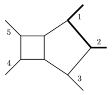
(a) Family ${\rm PB}_{A}$.

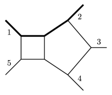
(b) Family ${\rm PB}_{B}$.

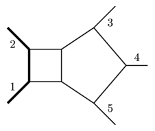
(c) Family ${\rm PB}_{C}$.

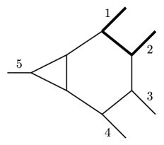
(d) Family ${\rm HT}_{A}$.

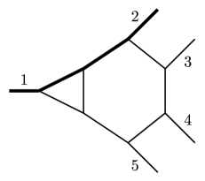
(e) Family ${\rm HT}_{B}$.

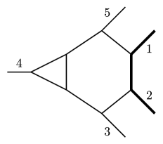
(f) Family ${\rm HT}_{C}$.

Figure 2: Integral families relevant for the leading-colour two-loop $gg\rightarrow t\bar{t}g$ amplitude. The hexagon-triangle (${\rm HT}$) families, in the second row, can be reduced to pentagon-box (${\rm PB}$) families, in the first row, except for 4 master integrals of ${\rm HT}_{B}$ which can instead be expressed as products of one-loop integrals. Four more families, $\mathrm{PB}_{A}^{\prime}$, $\mathrm{PB}_{B}^{\prime}$, $\mathrm{HT}_{A}^{\prime}$ and $\mathrm{HT}_{B}^{\prime}$, are obtained by exchanging $1\leftrightarrow 2$ and $3\leftrightarrow 5$ in $\mathrm{PB}_{A}$, $\mathrm{PB}_{B}$, $\mathrm{HT}_{A}$ and $\mathrm{HT}_{B}$, respectively.

With respect to Ref. Badger:2024fgb and section˜4.1, we remove from the master integrals the overall square-root normalisations. The next step is the Laurent expansion around $\epsilon=0$. For the rational coefficients of the master integrals this is done within the finite-field framework. The master integrals are instead expressed order by order in $\epsilon$ as polynomials in the set of special functions and transcendental constants defined in section˜4, as well as square roots originating from the different normalisation. We denote cumulatively the special functions and transcendental constants by $F$ and the nine square roots by $\sqrt{S}$. As a result, the mass-renormalised contracted amplitude takes the form

$$\sum_{\mathrm{pol.}}T_{i}^{\dagger}A^{(L)}_{\mathrm{mren}}=\sum_{s=-2L}^{4-2L}\sum_{j}\epsilon^{s}\;c_{ij,s}\bigl{(}\vec{d}\;\bigr{)}\;\mathrm{mon}_{j}\left(F,\sqrt{S}\right)+\mathcal{O}\left(\epsilon^{5-2L}\right)\,,$$ (24)

where $\mathrm{mon}_{j}$ denotes monomials of special functions $F$ and square roots $\sqrt{S}$, and we recall that $\vec{d}$ is the set of scalar invariants defined in eq.˜3. The finite remainder is obtained by subtracting the IR and remaining UV poles from the mass-renormalised amplitude as prescribed in eqs.˜7 and 8. To this end, we first express the UV and IR subtraction terms in the same set of special functions as the two-loop amplitude. The subtraction terms are then Laurent expanded in $\epsilon$ through the same order as the bare amplitude. The finite remainder of the contracted amplitude, $\sum_{\mathrm{pol.}}T_{i}^{\dagger}R^{(L)}$, is given by

$$\sum_{\mathrm{pol.}}T_{i}^{\dagger}R^{(L)}=\sum_{s=0}^{4-2L}\sum_{j}\epsilon^{s}\;r_{ij,s}\bigl{(}\vec{d}\;\bigr{)}\;\mathrm{mon}_{j}\left(F,\sqrt{S}\right)+\mathcal{O}\left(\epsilon^{5-2L}\right)\,.$$ (25)

We recall that the finite remainder admits the same colour and spin-basis decomposition as the bare amplitude as specified in eqs.˜5 and 12. We can further derive the helicity-dependent finite remainder $R^{(L)}$ in terms of special functions following eq.˜23, as

$$R^{(L)}(1^{+}_{\bar{t}},2^{+}_{t}, 3^{h_{3}}_{g},4^{h_{4}}_{g},5^{h_{5}}_{g};n_{1},n_{2})$$

$$=\sum_{i,j=1}^{32}\sum_{k}\sum_{s=0}^{4-2L}T_{i}^{++h_{3}h_{4}h_{5}}(n_{1},n_{2})\left(\Theta^{-1}\right)_{ij}\;\epsilon^{s}\;r_{jk,s}\bigl{(}\vec{d}\;\bigr{)}\mathrm{mon}_{k}\left(F,\sqrt{S}\right)+\mathcal{O}\left(\epsilon^{5-2L}\right)\,,$$ (26)

$$=\sum_{i}\sum_{s=0}^{4-2L}\epsilon^{s}\;\hat{r}^{h_{3}h_{4}h_{5}}_{i,s}(\{p\},n_{1},n_{2})\;\mathrm{mon}_{i}\left(F,\sqrt{S}\right)+\mathcal{O}\left(\epsilon^{5-2L}\right)\,,$$ (27)

where $\hat{r}^{h_{3}h_{4}h_{5}}_{i,s}(\{p\},n_{1},n_{2})$ is made of spinor brackets and scalar products involving external momenta $p_{i}$ and reference vectors $n_{i}$. In the case of the projected helicity finite remainder (cf. eq.˜14), we have

$$R^{(L)}(1^{+}_{\bar{t}},2^{+}_{t},3^{h_{3}}_{g},4^{h_{4}}_{g},5^{h_{5}}_{g};p_{a},p_{b}) =\sum_{i}\sum_{s=0}^{4-2L}\epsilon^{s}\;\tilde{r}^{h_{3}h_{4}h_{5}}_{i,s;ab}(\{p\})\;\mathrm{mon}_{i}\left(F,\sqrt{S}\right)+\mathcal{O}\left(\epsilon^{5-2L}\right)\,,$$ (28)

where $(p_{a},p_{b})\in\{(p_{3},p_{3}),(p_{3},p_{4}),(p_{4},p_{3}),(p_{4},p_{4})\}$ and the rational coefficients $\tilde{r}^{h_{3}h_{4}h_{5}}_{i,s;ab}$ are now expressed fully in terms of on-shell $gg\to t{\bar{t}}g$ kinematics.

Starting from the analytic expression of the contracted amplitudes $\sum_{\mathrm{pol.}}T_{i}^{\dagger}A^{(L)}$, the computation is organised as a dataflow graph where all rational operations among rational functions are performed numerically in a finite field within the framework FiniteFlow Peraro:2016wsq ; Peraro:2019svx . This includes in particular the IBP reduction to master integrals and the Laurent expansion of the rational coefficients. We simplify the IBP-reduction step by generating optimised systems of IBP relations with NeatIBP Wu:2023upw . The conversion of the contracted amplitudes into projected helicity amplitudes according to section˜3 requires a rational parameterisation of the external kinematics including the spinor brackets. For this purpose we use the momentum-twistor parameterisation defined in Ref. Badger:2022mrb , in terms of the variables

$$\vec{x}=\bigl{(}s_{34},t_{12},t_{23},t_{45},t_{51},x_{5123}\bigr{)}\,.$$ (29)

In this work, we obtain numerical results for the $gg\to t\bar{t}g$ helicity amplitude. In other words, we do not compute the analytic expression of the rational coefficients of the special function monomials, but obtain numerical values for them at sample phase-space points in the physical region. We set $\vec{d}$ at the chosen phase-space point and rationalise it, and carry out the computation from the unreduced mass-renormalised contracted amplitude, $\sum_{\mathrm{pol.}}T_{i}^{\dagger}A^{(L)}_{\mathrm{mren}}$, to obtain the corresponding representation in terms of special functions (cf. eq.˜24), numerically over finite fields. By putting together the values of the coefficients of the special-function monomials in sufficiently many prime fields, we can perform a rational reconstruction and obtain their values in $\mathbb{Q}$. The subsequent set of operations are done outside of the finite-field framework. We subtract the UV and IR poles from the mass-renormalised contracted amplitude to derive the finite remainder representation as in eq.˜25, where the special functions are kept symbolic while the corresponding rational coefficients are evaluated numerically at the chosen phase-space point, and carry out the conversion to the projected helicity finite remainder in eq.˜28 via momentum-twistor variables. As a result, we obtain numerical values of the coefficients of the special-function monomials, i.e., $\tilde{r}^{h_{3}h_{4}h_{5}}_{i,s;ab}(\{p\})$ in eq.˜28, for the three independent helicity configurations. The evaluation of the finite remainders is then completed by the evaluation of the special functions, which is discussed in section˜4.2.

4 Laurent expansion of the master integrals

In this section we discuss our method to express the master integrals in terms of a set of special functions designed to accomplish three key goals: the analytic subtraction of the UV/IR poles of the amplitudes, the simplification of the finite remainders, and a more efficient numerical evaluation with respect to what was previously available in the literature Badger:2022hno ; Badger:2024fgb . The starting point is the method of the so-called pentagon functions Gehrmann:2018yef ; Chicherin:2020oor ; Badger:2021nhg ; Chicherin:2021dyp ; Abreu:2023rco , which has proven extremely successful in the computation of two-loop five-particle amplitudes with no internal massive propagators (see also Refs. Henn:2022ydo ; Badger:2023xtl ; AH:2023ewe ; Henn:2024ngj ; Gehrmann:2024tds ; Liu:2024ont for the application of similar methods to other cases). This method applies to those cases where the basis $\vec{g}_{\rm F}$ of all relevant integral families $\mathrm{F}$ satisfies a differential equation (DE) in the canonical form Henn:2013pwa

$$\mathrm{d}\vec{g}_{\rm F}(X;\epsilon)=\epsilon\,\sum_{i}A_{i}\,\mathrm{d}\log W_{i}(X)\cdot\vec{g}_{\rm F}(X;\epsilon)\,,$$ (30)

where $X$ denotes the kinematic variables (in this case $X=\vec{d}$, cf. eq.˜3), $\epsilon=(4-D)/2$ is the dimensional regulator, $\mathrm{d}$ is the total differential w.r.t. $X$, the $A_{i}$’s are constant matrices with entries in $\mathbb{Q}$, and the $W_{i}(X)$’s are algebraic functions of $X$ called letters. The method allows us to write the solution to eq.˜30 in terms of a basis of special functions, i.e., of a set of algebraically independent special functions.

In this work, we initiate the extension of this approach to Feynman integrals which satisfy DEs in a form different from eq.˜30. We present our algorithm to construct a set of special functions to express the solution to non-canonical DEs in section˜4.1, and discuss how we evaluate them numerically in section˜4.2.

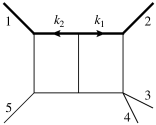
(a) $g_{15}$

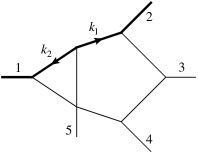
(b) $g_{19}$, $g_{20}$

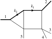
(c) $g_{35}$, $g_{36}$, $g_{37}$

Figure 3: Graphs representing the sectors of the family ${\rm PB}_{B}$ which contain master integrals that we did not express in terms of iterated integrals at order $\epsilon^{4}$. The external momenta are all outgoing, the thick line denotes the top, and the arrows indicate the momentum’s direction. The sub-captions list the relevant master integrals. They are defined by multiplying the scalar propagators associated with the graphs by the following numerators under the integral sign: $\displaystyle\begin{aligned} &N_{15}=\epsilon^{4}\,d_{15}^{2}\,(k_{2}+p_{2})^{2}+\ldots\,,\\ &N_{19}=\epsilon^{4}\,d_{45}\,\mathrm{tr}\bigl{(}\gamma_{5}\not{p}_{3}(\not{k}_{1}-\not{p}_{2}-\not{p}_{3})\not{p}_{4}\not{p}_{2}\bigr{)}\,,\\ &N_{20}=\epsilon^{4}\,d_{45}\,\mathrm{tr}\bigl{(}\not{p}_{3}(\not{k}_{1}-\not{p}_{2}-\not{p}_{3})\not{p}_{4}\not{p}_{2}\bigr{)}\,,\end{aligned}\qquad\begin{aligned} &N_{35}=\epsilon^{4}\,d_{15}(d_{12}+m_{t}^{2})\,,\\ &N_{36}=2\,\epsilon^{4}\,\sqrt{(d_{15}-d_{34})^{2}-2d_{34}m_{t}^{2}}\,(k_{1}\cdot p_{1})\,,\\ &N_{37}=2\,\epsilon^{4}(2\epsilon-1)\,d_{15}\,(k_{2}\cdot p_{2})\,,\end{aligned}$ where the ellipsis denotes sub-sector terms. We recall that the sector in figure (b) contains the nested square root, whereas the sector in figure (c) involves elliptic functions.

4.1 Construction of a (over-complete) basis of special functions

We begin by quickly reviewing the method of Ref. Abreu:2023rco . The inputs are canonical DEs for all the relevant one- and two-loop integral families ${\rm F}$, and numerical ‘boundary’ values of all basis integrals $\vec{g}_{\rm F}$ at an arbitrary phase-space point $X_{0}$. Using this information, one writes the solution to the canonical DEs in terms of Chen iterated integrals Chen:1977oja (see e.g. Ref. Abreu:2022mfk for a review), order by order in $\epsilon$,

$$\vec{g}_{\rm F}(X;\epsilon)=\sum_{k\geq 0}\epsilon^{k}\,\vec{g}^{\,(k)}_{\rm F}(X)\,.$$ (31)

We truncate the expansion at the highest order required to compute two-loop amplitudes up to their finite part. By reducing the amplitude to master integrals as discussed in section˜3, we know that this is $k=4$. The order in $\epsilon$ in the canonical case matches the transcendental weight, and the weight-0 $\epsilon$-coefficients $\vec{g}_{\rm F}^{(0)}$ are constant and rational. Next, we exploit the $\mathbb{Q}$-linear independence of iterated integrals and the shuffle product to select, out of all $\epsilon$-coefficients $\{\vec{g}_{\rm F}^{(k)},\forall\,\mathrm{F},i=1,2,3,4\}$, a subset of elements which are algebraically independent. We denote them by $\{F_{i}^{(k)}\}$, where $k$ denotes the transcendental weight. This is achieved by Gaussian elimination, with an ordering which is chosen to impose certain useful criteria. In particular, products of lower-weight $\epsilon$-coefficients are preferred over higher-weight ones, and one-loop $\epsilon$-coefficients over two-loop ones. As a result, the number of higher-weight functions is minimised, and we know a priori that the $\epsilon$-poles of the amplitudes contain only the subset of functions coming from the one-loop integrals. More criteria are imposed on a case-by-case basis, e.g. to make manifest the cancellation of certain letters from the amplitudes/finite remainders. We perform this procedure first at the symbol level Goncharov:2010jf , i.e., by setting to zero all $\vec{g}^{(k)}_{\rm F}(X_{0})$ for $k>0$. The result is then lifted to iterated integral by ansatzing. Finally, the outputs are:

• a list of algebraically independent $\epsilon$-coefficients, $\{F_{i}^{(k)}\}$, dubbed pentagon functions,

• the expression of all $\epsilon$-coefficients $\vec{g}_{\rm F}^{(k)}(X)$ as polynomials in the ring generated by the pentagon functions, $\zeta_{2}$ and $\zeta_{3}$, with coefficients in $\mathbb{Q}$,

• polynomial relations among the values $\vec{g}_{\rm F}^{(k)}(X_{0})$ with $k>0$, which are checked numerically.

The method summarised above applies straightforwardly to the one-loop family ($\mathrm{P}_{A}$) and to three of the five two-loop families relevant for $t\bar{t}j$-production at leading colour, namely $\mathrm{PB}_{A}$, $\mathrm{PB}_{A}^{\prime}$ and $\mathrm{PB}_{C}$. We recall that the superscript ^′ in the family name denotes the permutation $(1\to 2,2\to 1,3\to 5,4\to 4,5\to 3)$ of the external legs. The canonical DEs for the permuted families are obtained by permuting the DEs for the families in the standard ordering derived in Refs. Badger:2022hno ; Badger:2024fgb . In doing this, we add 28 new letters and two new square roots (permutations of $\Lambda_{1}$ and $\Lambda_{3}$) to the alphabet of Ref. Badger:2024fgb . The available DEs for the two remaining families (${\rm F}=\mathrm{PB}_{B},\mathrm{PB}_{B}^{\prime}$), instead, have the non-canonical form

$$\mathrm{d}\vec{g}_{\rm F}(X;\epsilon)=\Omega_{\rm F}(X;\epsilon)\cdot\vec{g}_{\rm F}(X;\epsilon)\,,$$ (32)

where the connection matrix $\Omega_{\rm F}(X;\epsilon)$ is a degree-2 polynomial in $\epsilon$,

$$\Omega_{\rm F}(X;\epsilon)=\sum_{k=0}^{2}\epsilon^{k}\,\Omega^{(k)}_{\rm F}(X)\,,$$ (33)

with

$$\Omega_{\rm F}^{(k)}(X)=\sum_{i}A^{({\rm F})}_{k,i}\,\mathrm{d}\log W_{i}(X)+\sum_{j}B^{({\rm F})}_{k,j}\,\omega_{j}(X)\,.$$ (34)

Here, $\omega_{j}(X)$ are $\mathbb{Q}$-linearly independent non-logarithmic one-forms. Importantly, however, the deviation from the canonical form is restricted to a small subset of MIs: $S=\{15,19,20,35,36,37\}$. We recall their definition from Ref. Badger:2024fgb in fig.˜3. Explicitly, we have that

• the entry $(\Omega_{\rm F})_{ab}$ is canonical for $a,b\neq S$, i.e., it is $\epsilon$-factorised and involves $\mathrm{d}\log$’s only;

• only the derivatives of the 37th MI are quadratic in $\epsilon$, i.e., $[A_{2,i}^{(\rm F)}]_{ab}=0=[B_{2,i}^{(\rm F)}]_{ab}$ for $a\neq 37$.

We recall from Ref. Badger:2024fgb that the MIs #19 and 20 of ${\rm PB}_{B}$ belong to the sector which involves a nested square root, whereas the MIs #35–37 are those of the sector containing elliptic functions. The 15th MI, on the other hand, is somewhat mysterious: it is in fact canonical on the maximal cut, and its derivatives contain non-logarithmic one-forms not only in correspondence with the elliptic MIs — as is expected — but also in correspondence with non-elliptic MIs. It would be interesting to investigate whether this feature can be removed with a basis transformation.

In addition to the DEs, another piece of information we will make use of is the list of which $\epsilon$-coefficients $\vec{g}_{\rm F}^{\,(k)}(X)$ vanish. We determine it by performing a number of numerical evaluations of the MIs with AMFlow Liu:2017jxz ; Liu:2022chg at random phase-space points. An important feature is that the MIs of the sectors which are not canonical on the maximal cut (in this case, those in $S\backslash\{15\}$) are non-zero only starting from order $\epsilon^{4}$. In other words, they start to contribute only in the finite remainder of the two-loop scattering amplitude. On the one hand, it is expected that this is the case, as the $\epsilon$-poles of the amplitudes are determined by the one-loop amplitudes, which are polylogarithmic, as discussed in section˜2. On the other hand, this is not manifest for an arbitrary choice of MIs, and effort was put in Ref. Badger:2024fgb to satisfy this condition. Nonetheless, the 15th MI is non-zero already at order $\epsilon^{0}$. We will see below that the non-polylogarithmic one-forms drop out from the solution up to order $\epsilon^{3}$ thanks to a conspiracy among the boundary values.

We are now ready to extend the method of Ref. Abreu:2023rco . We assume that $\mathrm{F}={\rm PB}_{B}$ and neglect the family subscript to simplify the notation. The same procedure works for ${\rm PB}_{B}^{\prime}$ as well. First, we plug the $\epsilon$-expansion of eq.˜31 into eq.˜32. The polynomial $\epsilon$-dependence of the connection matrix implies an iterative system of DEs for the $\epsilon$-coefficients,

$$\mathrm{d}\vec{g}^{\,(k)}(X)=\Omega^{(0)}(X)\cdot\vec{g}^{\,(k)}(X)+\Omega^{(1)}(X)\cdot\vec{g}^{\,(k-1)}(X)+\Omega^{(2)}(X)\cdot\vec{g}^{\,(k-2)}(X)\,,$$ (35)

for $k\geq 0$, with $\vec{g}^{\,(-2)}(X)=0=\vec{g}^{\,(-1)}(X)$. Next, we drop all $\epsilon$-coefficients which we have determined numerically to be zero. We find that the $\vec{g}^{\,(0)}(X)$’s are constant. We can thus rationalise the numerical boundary values, and plug them into the DEs for $\vec{g}^{\,(1)}(X)$. As a result, the latter take the canonical form,

$$\mathrm{d}\vec{g}^{\,(1)}(X)=\sum_{i}A_{1,i}\,\mathrm{d}\log W_{i}(X)\cdot\vec{g}^{\,(0)}(X)\,.$$ (36)

We can therefore solve eq.˜36 in terms of iterated integrals, and substitute the resulting expressions of $\vec{g}^{\,(0)}(X)$ and $\vec{g}^{\,(1)}(X)$ into the DEs for $\vec{g}^{\,(2)}(X)$. The derivatives of the 15th MI however appear to contain non-logarithmic one-forms, e.g.

$$\mathrm{d}g_{15}^{(2)}(X)=\frac{1}{24}\Bigl{[}12\,g^{(1)}_{103}(X_{0})+8\,g^{(1)}_{110}(X_{0})+4\,g^{(1)}_{111}(X_{0})+3\,g^{(1)}_{118}(X_{0})-48\,g^{(1)}_{63}(X_{0})\Bigl{]}\,\omega_{2}(X)+\ldots\,.$$ (37)

This obstruction is removed by a conspiracy of the boundary values: all combinations of boundary values which multiply non-logarithmic one-forms vanish. We stress that we do not need to resort to the PSLQ algorithm PSLQ to find such relations among the boundary values. It suffices to look at the coefficients of the $\omega_{i}(X)$’s in the derivatives of $g_{15}^{(2)}(X)$, and check numerically that they vanish. Interestingly, the constraints on the boundary values obtained this way are a subset of those returned by the algorithm of Ref. Abreu:2023rco applied to $\vec{g}^{\,(1)}(X)$. Once the non-logarithmic one-forms are removed, the DEs for $\vec{g}^{\,(2)}(X)$ take the canonical form as well, and can be solved in terms of iterated integrals. We proceed similarly for $\vec{g}^{\,(3)}(X)$ and for the $g^{\,(4)}_{i}(X)$ with $i\notin S$. As a result, we have iterated-integral expressions for all $\epsilon$-coefficients $\vec{g}^{\,(k)}(X)$ with $k=1,2,3$, and at $\epsilon^{4}$ for $g^{\,(4)}_{i}(X)$ with $i\notin S$.

We apply the same procedure to ${\rm PB}_{B}^{\prime}$. The permutation of the DEs for ${\rm PB}_{B}$ yields 63 new one-forms, in addition to the 63 defined in Ref. Badger:2024fgb . Out of these, only 76 are relevant for the solutions truncated at order $\epsilon^{4}$.

Finally, we apply the algorithm of Ref. Abreu:2023rco to construct a basis of special functions out of the $\epsilon$-coefficients for which we have an iterated-integral representation. These are $\vec{g}_{\rm F}^{(k)}$ for $k\in\{1,2,3,4\}$ and ${\rm F}\in\{{\rm P}_{A},{\rm PB}_{A},{\rm PB}_{A}^{\prime},{\rm PB}_{C}\}$, $\vec{g}_{\rm F}^{(k)}$ for $k\in\{1,2,3\}$ and ${\rm F}\in\{{\rm PB}_{B},{\rm PB}_{B}^{\prime}\}$, and $g_{\rm F,i}^{(4)}$ for ${\rm F}\in\{{\rm PB}_{B},{\rm PB}_{B}^{\prime}\}$ and $i\notin\{15,19,20,35,36,37\}$. The resulting number of algebraically independent functions and their breakdown in transcendental weight are shown in table˜1.

transcendental weight	1	2	3	4	4*	all
# of functions	6	8	45	166	12	237

Table 1: Number of special functions in our expression of the one- and two-loop amplitudes for $t\bar{t}j$ production at leading colour, broken down by transcendental weight. We label by 4* the non-polylogarithmic functions appearing in the MIs at order $\epsilon^{4}$.

The 12 remaining $\epsilon$-coefficients, namely $g_{\rm F,i}^{(4)}$ for ${\rm F}\in\{{\rm PB}_{B},{\rm PB}_{B}^{\prime}\}$ and $i\in\{15,19,20,35,36,37\}$, satisfy coupled DEs involving non-logarithmic one-forms. Since we cannot solve the latter in terms of iterated integrals, we have no handle over the relations they might satisfy. However, it is reasonable to expect that only a limited number of relations can exist among these functions, as they are divided into subsets with different analytic features (the nested square root, the elliptic curve, or both). Regardless of this, since they are comparatively few and contribute solely to the two-loop finite remainders, we can add them to the generating set of special functions and still achieve the objectives we set at the start of this section. We dub these functions non-polylogarithmic, meaning that they do not have a representation in terms of iterated integrals with logarithmic integration kernels. We label them by $F^{(4^{*})}_{i}$, for $i=1,\ldots,12$, with an asterisk to remind us that, while these functions appear in the MIs at order $\epsilon^{4}$, they do not have a transcendental weight.

Finally, we have completed the construction of a (potentially over-complete) basis of special functions. All one- and two-loop MIs relevant for $t\bar{t}j$ production at leading colour are expressed, order by order in $\epsilon$ up to $\epsilon^{4}$, as polynomials in the ring generated by the basis functions and Riemann zeta values ($\zeta_{2}$ and $\zeta_{3}$). For example, we spell out illustrative terms in the expression of the 15th MI of ${\rm PB}_{B}$:

$$\begin{aligned} g_{15}(X;\epsilon)=\phantom{}&\frac{1}{48}+\frac{\epsilon}{24}\left(F^{(1)}_{1}-2\,F^{(1)}_{2}+2\,F^{(1)}_{4}-2\,F^{(1)}_{6}\right)\\ &-\frac{1}{48}\epsilon^{2}\left[7\,F^{(2)}_{1}+7\,F^{(2)}_{3}+\frac{25}{4}\zeta_{2}-\frac{15}{4}\,\left(F^{(1)}_{1}\right)^{2}+15\,F^{(1)}_{1}\,F^{(1)}_{2}-8\,\left(F^{(1)}_{2}\right)^{2}+\ldots\right]\\ &+\frac{1}{8}\epsilon^{3}\left[F^{(3)}_{5}+\frac{820}{9}\zeta_{3}+\frac{7}{12}\zeta_{2}F^{(1)}_{2}-\left(F^{(1)}_{2}\right)^{3}+5\,\left(F^{(1)}_{3}\right)^{2}F^{(1)}_{5}+6\,F^{(1)}_{1}F^{(1)}_{2}F^{(1)}_{6}+\ldots\right]\\ &+\epsilon^{4}\,F^{(4^{*})}_{1}+\mathcal{O}\left(\epsilon^{5}\right)\,,\end{aligned}$$ (38)

where we omit the dependence of $F^{(i)}_{j}$ on $X$. As in the fully canonical cases, the special functions inherit from the MIs a parity (either even or odd) with respect to the square roots appearing in the alphabet. We list the odd functions and the corresponding square roots in our ancillary files ancillary .

We will see in section˜5 that, albeit potentially over-complete, the special function basis allows us to subtract the UV/IR poles of the amplitudes analytically, and leads to a dramatic simplification of the expression of the amplitudes with respect to a representation in terms of MIs. The next subsection will instead be devoted to the numerical evaluation of the special function basis.

We conclude this section by highlighting the conditions underpinning our new method:

• the connection matrices are polynomial in $\epsilon$, and are expressed in terms of $\mathrm{d}\log$’s and $\mathbb{Q}$-linearly independent non-logarithmic one-forms;

• we have sufficiently many numerical values of the MIs to establish reliably which $\epsilon$-coefficients vanish and to check the relations returned by the algorithm of Ref. Abreu:2023rco ;

• the MIs whose DEs are not in canonical form on the maximal cut are non-zero only starting from the highest $\epsilon$-order that is required for the amplitude computation.

The scope of applicability of our new method is therefore significantly larger than that of the previous approach Abreu:2023rco .

4.2 Numerical evaluation of the special functions

In the final part of this section, we discuss the numerical evaluation of special functions and propose a strategy to address the main bottleneck in this part of the computation: the numerical evaluation of the non-polylogarithmic special functions, $\{F^{(4^{*})}_{i}\}_{i=1}^{12}$, for which no efficient method is currently known. Our goal is thus to minimise the impact of the non-polylogarithmic functions on the overall numerical evaluation time. All special functions for which we have a representation in terms of iterated integrals are in fact suitable to be evaluated numerically with the approach discussed in Refs. Caron-Huot:2014lda ; Gehrmann:2018yef ; Chicherin:2020oor . The latter is based on constructing a representation in terms of logarithms and dilogarithms for the weight-1 and 2 functions, and one-fold integral representations at weights 3 and 4. The one-fold integrations are then performed numerically in a dedicated C++ library PentagonFunctions:cpp . Based on the previous successful applications to two-loop five-particle integrals, it is reasonable to expect that this approach will yield an efficient and stable numerical evaluation. We leave this to future work, and limit ourselves to giving an explicit expression only for the weight-1 functions:

$$\begin{aligned} F^{(1)}_{1}&=\log(m_{t}^{2})\,,&F^{(1)}_{2}&=\log\bigl{[}2(d_{12}+m_{t}^{2})\bigr{]}-\mathrm{i}\pi\,,\quad&F^{(1)}_{3}&=\log(2d_{23})-\mathrm{i}\pi\,,\\ F^{(1)}_{4}&=\log(-2d_{34})\,,\quad&F^{(1)}_{5}&=\log(2d_{45})-\mathrm{i}\pi&F^{(1)}_{6}&=\log(-2d_{15})\,,\end{aligned}$$ (39)

where the logarithms are well-defined in the $45\to 123$ scattering channel. We need eq.˜39 in order to express the IR/UV subtraction terms in the same special function basis as the amplitudes. For the non-polylogarithmic functions, we instead construct a minimal system of DEs, which we then solve by means of generalised power series. A detailed performance analysis of this approach is provided at the end of the section.

We now focus on the construction of the system of differential equations for the non-polylogarithmic functions $\{F^{(4^{*})}_{i}\}_{i=1}^{12}$ Badger:2021nhg ,

$$\mathrm{d}\vec{G}(X)=M(X)\cdot\vec{G}(X)\,,$$ (40)

where the connection matrix has the form

$$M(X)=\sum_{i}A_{i}\,\mathrm{d}\log W_{i}(X)+\sum_{j}B_{j}\,\omega_{j}(X)\,.$$ (41)

In eq.˜40, $\vec{G}$ is a list of polynomials of special functions and transcendental constants constructed as follows. We start from the non-polylogarithmic functions. Next, we add all $\mathbb{Q}$-linearly independent combinations of monomials of special functions required to express the derivatives of the non-polylogarithmic functions, which we know thanks to the DEs for the MIs. We then take the differential of the newly added functions, and iterate until we reach the differential of weight-1 functions, which requires solely a weight-0 function (chosen to be $1$) to be written. In addition to the 12 non-polylogarithmic functions, the resulting $\vec{G}$ contains 40, 25, 6 and 1 special function polynomials of weight-3, 2, 1 and 0, respectively, for a total of 84 elements. For the sake of clarity, we spell out a few terms of $\vec{G}$,

$$\vec{G}=\Bigl{(}F^{(4^{*})}_{1}\,,\ldots,F^{(4^{*})}_{12}\,,\ldots,F^{(3)}_{39}\,,\ldots,F^{(3)}_{7}+F^{(1)}_{1}F^{(2)}_{4}-2F^{(1)}_{6}F^{(2)}_{4}\,,\ldots,\zeta_{3}\,,\ldots,F^{(1)}_{6}\,,1\Bigr{)}^{\top}\,,$$ (42)

and of the differential of $F^{(4^{*})}_{1}$,

$$\begin{aligned} \mathrm{d}F^{(4^{*})}_{1}=\phantom{}&\omega_{1}\,F^{(4^{*})}_{4}+\omega_{2}\,F^{(4^{*})}_{6}-\frac{1}{2}\left(\omega_{31}+\frac{1}{2}\,\mathrm{d}\log W_{69}\right)F^{(3)}_{39}\\ &+\frac{1}{4}\,\mathrm{d}\log W_{70}\left(F^{(3)}_{7}+F^{(1)}_{1}F^{(2)}_{4}-2\,F^{(1)}_{6}F^{(2)}_{4}\right)+\ldots\,.\end{aligned}$$ (43)

We display in fig.˜4 the non-zero entries of the connection matrix $M(X)$, distinguishing between logarithmic (blue) and non-logarithmic (red) one-forms. The three addends on the first row on the right-hand side of eq.˜43 involve non-logarithmic one-forms and correspond to the red dots on the first row of fig.˜4. The addend on the second row instead corresponds to the first blue dot on the first row of fig.˜4. In fig.˜4 one can see that the restriction of the connection matrix to the functions with transcendental weight up to 3 is strictly upper triangular, as expected. The non-polylogarithmic functions are instead coupled to themselves, and in the top left block one can distinguish two sub-blocks associated with the two permutations of ${\rm PB}_{B}$. Two functions, $F^{(4^{*})}_{6}$ and $F^{(4^{*})}_{12}$, couple also to weight-2 functions; they originate from the 37th MI of ${\rm PB}_{B}$ and ${\rm PB}_{B}^{\prime}$, respectively, whose derivatives are quadratic in $\epsilon$.

Figure 4: Matrix plot displaying the non-zero entries of the connection matrix in eq.˜40. Blue dots indicate non-zero entries involving logarithmic one-forms, while the red entries contain also non-logarithmic special functions. The solid black lines separate subsets of functions with different transcendental weight, as shown on the left, with $4^{*}$ denoting the non-polylogarithmic special functions.

Finally, we solve the DEs for the special functions $\vec{G}$ by means of generalised power-series expansions Moriello:2019yhu , as implemented in DiffExp Hidding:2020ytt . This approach has several advantages as compared to solving via generalised power-series the DEs for the MIs. Firstly, the DEs for the special functions do not depend on $\epsilon$. Secondly, while the DEs for the MIs contain information regarding the entire $\epsilon$ expansion of the solution, the DEs for the special functions contain only the letters and one-forms which are required up to the chosen truncation order. Finally, the size of the system for the non-polylogarithmic special functions (84) is smaller than the number of MIs of each of the relevant two-loop families (121 each for ${\rm PB}_{B}$ and ${\rm PB}_{B}^{\prime}$), let alone of their union. These observations lead us to believe that the method we propose represents a substantial improvement over what was previously available in the literature for this class of integrals.

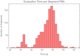
(a) ${\rm PB}_{A}$

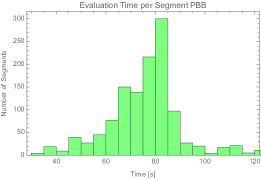
(b) ${\rm PB}_{B}$

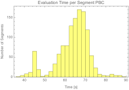
(c) ${\rm PB}_{C}$

Figure 5: Distributions of the evaluation time per segment in the solution of the DEs for the MIs of each family with DiffExp.

In order to confirm this expectation, we perform some benchmark evaluations to compare the efficiency of the three different approaches now on the market, all making use of generalised power series as implemented in DiffExp: the solution to the DEs for the MIs of each separate family, for the non-polylogarithmic special functions (cf. eq.˜40), and for all special functions. While the more efficient routine for the polylogarithmic functions is unavailable, we can in fact apply the method discussed above also to all 237 special functions, rather than just the non-polylogarithmic ones. The dimension of the corresponding system of DEs is 366, with the 12 non-polylogarithmic functions followed by 166, 151, 30, 6 and 1 polylogarithmic functions with transcendental weights 4, 3, 2, 1 and 0, respectively.

As a benchmark, we use the average evaluation time per segment in the generalised power series expansion. We emphasise that the evaluation time per phase-space point strongly depends on the segmentation of the path within the generalised power series expansion method Moriello:2019yhu ; Hidding:2020ytt . An efficient evaluation routine aimed at a large number of phase-space points should thus also aim to minimise the number of segments (see e.g. Ref. Abreu:2020jxa ). Therefore, the evaluation time per segment is a more reliable indicator of the method’s performance. The analysis is conducted using a random sample of physical phase-space points in the $s_{45}$ channel, encompassing a total of approximately $1$K segments in each case, starting from the boundary point

$$\vec{d}_{0}=\bigl{(}2,1,-1,5,-2,1\bigr{)}\,.$$ (44)

We restrict our analysis to points which can be reached from $\vec{d}_{0}$ by a straight line in the $\vec{d}$-space without exiting the $s_{45}$ channel. The values of all MIs at $\vec{d}_{0}$ are provided in Ref. Badger:2024fgb . The results on this analysis are summarised in the histograms in figs.˜5 and 6. In fig.˜5 we show the distribution of the evaluation time per segment in the solution of the DEs for all sets of MIs, while in fig.˜6 we display the same for the full set of 366 special functions (fig.˜6(a)), and for the non-polylogarithmic functions alone (fig.˜6(b)).

	${\rm PB}_{A}$	${\rm PB}_{B}$	${\rm PB}_{C}$	all MIs	special func. (all)	special func. (non-polylog.)
$\langle T\rangle$	$43\,s$	$77\,s$	$66\,s$	$309\,s$	$297\,s$	$16\,s$
$\sigma$	$7\,s$	$17\,s$	$14\,s$	$27\,s$	$65\,s$	$3\,s$

Table 2: Average time per segment and standard deviation for the solution of the DEs for the MIs of each 2-loop family, cumulatively for all 2-loop MIs, for all special functions, and for the non-polylogarithmic special functions alone. The time for all MIs keeps into account that ${\rm PB}_{A}$ and ${\rm PB}_{B}$ are needed in two permutations of the external legs, and that the time for the one-loop family (${\rm P}_{A}$) is $\approx\,2s$.

The average evaluation time per segment and the standard deviation in each case are shown in table˜2. These data do not indicate a significant improvement in the solution of the DEs for all special functions over those for the MIs. Indeed, the cumulative evaluation time per segment of the MIs of all relevant families is comparable to that of the special functions. However, the average time per segment for the non-polylogarithmic system, of $\approx 16\,s$, is significantly smaller than that for any set of two-loop MIs. This result confirms the soundness of our strategy. Namely, we can reduce substantially the bottleneck of the numerical evaluation of the non-polylogarithmic functions by constructing a minimal system of DEs for them, which are then solved using the generalised power series method. The polylogarithmic functions are instead to be evaluated numerically using the approach discussed in Refs. Caron-Huot:2014lda ; Gehrmann:2018yef ; Chicherin:2020oor ; PentagonFunctions:cpp .

(a) All special functions

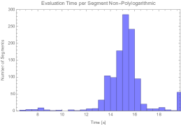
(b) Non-polylogarithmic special functions

Figure 6: Distributions of the evaluation time per segment in the solution of the DEs for all special functions and for the non-polylogarithmic functions alone with DiffExp.

We provide in our ancillary files ancillary

• the expression of the master integrals in terms of special functions,

• the square-root parity of the special functions,

• systems of DEs for both the complete and the non-polylogarithmic sets of special functions, including boundary values at the point in eq.˜44,

• a Mathematica script to solve the DEs for the special functions using DiffExp.

5 Results

Helicity	$R^{(0),[1]}$	$R^{(0),[2]}$	$R^{(0),[3]}$	$R^{(0),[4]}$
$+++$	$0.26326-0.0097514\,\mathrm{i}$	$0$	$0$	$0$
$+-+$	$5.9619-0.16047\,\mathrm{i}$	$0$	$0$	$-0.31659-0.097935\,\mathrm{i}$
$++-$	$-5.9575+0.0089231\,\mathrm{i}$	$-12.606-0.067440\,\mathrm{i}$	$4.6564+0.024911\,\mathrm{i}$	$-1.9692-0.010535\,\mathrm{i}$
Helicity	$R^{(1),[1]}/R^{(0),[1]}$	$R^{(1),[2]}/R^{(0),[1]}$	$R^{(1),[3]}/R^{(0),[1]}$	$R^{(1),[4]}/R^{(0),[1]}$
$+++$	$38.396-5.8002\,\mathrm{i}$	$71.982-4.0653\,\mathrm{i}$	$-14.289+0.70866\,\mathrm{i}$	$17.909-0.39528\,\mathrm{i}$
$+-+$	$19.221-8.4151\,\mathrm{i}$	$-4.8506+4.8015\,\mathrm{i}$	$0.67096-0.09959\,\mathrm{i}$	$-1.2201+2.1594\,\mathrm{i}$
$++-$	$20.369-19.991\,\mathrm{i}$	$41.522-41.969\,\mathrm{i}$	$-15.990+15.739\,\mathrm{i}$	$6.2964-6.4584\,\mathrm{i}$
Helicity	$R^{(2),[1]}/R^{(0),[1]}$	$R^{(2),[2]}/R^{(0),[1]}$	$R^{(2),[3]}/R^{(0),[1]}$	$R^{(2),[4]}/R^{(0),[1]}$
$+++$	$882.48-91.619\,\mathrm{i}$	$2489.7-266.72\,\mathrm{i}$	$-492.28+8.1003\,\mathrm{i}$	$593.35-87.569\,\mathrm{i}$
$+-+$	$414.16-206.87\,\mathrm{i}$	$-171.78+189.69\,\mathrm{i}$	$25.226-1.5639\,\mathrm{i}$	$-54.820+95.716\,\mathrm{i}$
$++-$	$332.97-646.02\,\mathrm{i}$	$623.01-1325.1\,\mathrm{i}$	$-259.14+512.33\,\mathrm{i}$	$89.185-198.65\,\mathrm{i}$

Table 3: Values of the tree-level helicity sub-amplitudes $R^{(0),[i]}$ and of the finite remainders of the one- and two-loop helicity sub-amplitudes, $R^{(1),[i]}$ and $R^{(2),[i]}$ respectively, as defined by eq.˜12 with the replacement $A\rightarrow R$. The one- and two-loop sub-amplitudes are normalised by the tree-level sub-amplitude $R^{(0),[1]}$. All sub-amplitudes are evaluated at the phase-space point specified in eqs.˜45 and 46. We drop the logarithms of the renormalisation and factorisation scales.

In this section, we present benchmark values of the two-loop helicity finite remainders for $gg\to t{\bar{t}}g$ in the leading colour approximation. These are obtained by putting together the values of the special functions, obtained as discussed in section˜4.2, and those of the rational coefficients of the finite remainders, resulting from the procedure outlined in section˜3. In table˜3 we give the values of the finite remainders of the helicity sub-amplitudes,

$$R^{(2),[i]}\qquad\forall\,i\in\{1,\cdots,4\}\,,$$

obtained by replacing $A$ with $R$ in eq.˜12 with the same superscripts, and solving for $R^{(2),[i]}$ at the selected phase-space point for all the independent helicity configurations of the gluons. We normalised the values by the tree-level sub-amplitude $R^{(0),[1]}$. For completeness, we also provide in table˜3 the values of the tree-level helicity sub-amplitudes and of the one-loop finite remainders. In order to facilitate future comparisons, we provide in the ancillary files higher-precision values of the finite remainders, together with the values of the subtracted IR and UV poles needed to recover the mass-renormalised amplitudes ancillary .

We generated physical phase-space points by parameterising the external momenta in terms of energies and angles, and by sampling randomly the latter. Starting from the physical momenta, we compute the corresponding values of the scalar invariants, which we rationalise in order to employ the finite-field setup. The point chosen for the sub-amplitudes evaluation in table˜3 is given by

$$\begin{aligned} &d_{12}=\frac{1617782845110651539}{15068333897971200000}\,,\qquad&&d_{23}=\frac{335}{1232}\,,\qquad&&d_{34}=-\frac{5}{32}\,,\\ &d_{45}=\frac{3665}{7328}\,,\qquad&&d_{15}=-\frac{45}{1408}\,,\qquad&&m_{t}^{2}=\frac{376940175237098461}{15068333897971200000}\,,\end{aligned}$$ (45)

with

$$\mathrm{tr}_{5}=\mathrm{i}\,\frac{\sqrt{582950030096630501}}{426229309440}\,.$$ (46)

The corresponding values of the momentum-twistor variables can be found in our ancillary files ancillary .

The values of special functions and master integrals are cross-checked among the three evaluation strategies discussed in section˜4.2. Our results for the rational coefficients are instead validated by verifying the gauge invariance of the amplitudes and by comparing the poles with the predictions from UV renormalisation and IR subtraction as discussed in section˜2. Furthermore, we crosschecked the results presented in table˜3—which were obtained using the projector method described in section˜3—against an independent calculation in which we reduce directly the helicity amplitudes in terms of momentum-twistor variables. For more details on this approach, see Refs. Badger:2021owl ; Badger:2021imn ; Badger:2021ega ; Badger:2023mgf ; Brancaccio:2024map .

Although we have not obtained fully analytic results, within the finite-field framework we could already gather some information on the complexity of the rational coefficients of both the master integrals and the special function monomials. We observe that the maximum polynomial degree of the rational coefficients goes down by $30\%$ when using our special-function representation of the master integrals with respect to computing the amplitude in terms of master integrals. This simplification shows the importance of Laurent-expanding the master integrals and expressing the coefficients of the expansion in terms of a basis of special functions. Furthermore, five weight-4 special functions ($F^{(4)}_{i}$ with $i\in\{24,34,98,127,151\}$) drop out of the two-loop finite remainders, while all the other special functions—including the non-polylogarithmic ones—appear independently.

6 Conclusions

In this article we have computed the two-loop helicity finite remainders for the production of a pair of on-shell top quarks in association with a gluon in gluon fusion ($gg\to t\bar{t}g$) at benchmark physical phase-space points. The helicity formalism we employed retains the complete information on the spin state of the top quarks, so that their decays can be included straightforwardly in the narrow-width approximation.

In order to achieve this result, we developed a new strategy to express the master integrals in terms of a (potentially over-complete) basis of special functions by solving the associated differential equations without requiring them to be in the canonical form. Elliptic functions are in fact known to appear in the solution, and a canonical form of the DEs for all two-loop master integrals is not available. We used numerical evaluations to determine which terms of the master integrals are zero, and exploited this information to extract the polylogarithmic part of the solution to the DEs and construct a basis of special functions to express it using known techniques Abreu:2023rco . The remaining non-polylogarithmic special functions are treated as independent, but are few and only appear in the finite part of the two-loop amplitudes. The latter property is necessary to maintain consistency with the universal pole structure, which cannot include any elliptic functions, but is hidden with an arbitrary choice of master integrals. Furthermore, we observe that solving the minimal subset of DEs which define the few non-polylogarithmic functions using generalised power series Moriello:2019yhu ; Hidding:2020ytt is significantly faster than solving the larger system satisfied by the full set of special functions or by the two-loop master integrals. This observation suggests that an efficient numerical evaluation may be achieved as follows. The subset of polylogarithmic special functions can be evaluated numerically with the method applied to the pentagon functions Caron-Huot:2014lda ; Gehrmann:2018yef ; Chicherin:2020oor , which is expected to yield a comparatively negligible evaluation time. This will require deriving a dedicated representation of the special functions, but the methodology is well understood and we expect the application to be straightforward. Only for the 12 non-polylogarithmic functions, then, we would need to resort to generalised power series. We leave to future work the optimisation of this part of the evaluation to target a large number of phase-space points by recycling iteratively the values obtained with previous evaluations (see e.g. Ref. Abreu:2020jxa ) and tuning the parameters of the algorithm (working precision, expansion order, etc.).

The representation of the master integrals in terms of special functions also leads to a major simplification of the finite remainders, which we evaluated numerically with a routine based on finite-field sampling in FiniteFlow to overcome the high algebraic complexity of the rational coefficients accompanying the special functions.

This work paves the way to achieve a fully analytical computation of the two-loop amplitudes required to describe $t\bar{t}$ + jet production at the LHC at NNLO in QCD. Furthermore, we expect that our method to extract the polylogarithmic part of the solution to non-canonical differential equations will find application in other computations in which a canonical form is currently out of reach.

Appendix A Renormalisation factors and infrared pole operators

In this appendix we list all terms that are needed to renormalise the amplitude according to eqs.˜6 and 7 and to cancel the IR singularities as described in eq.˜8. The leading-colour mass counterterms in the integral representation are given by Badger:2021owl

$$\begin{aligned} \delta Z_{m}^{(1)}={}&N_{c}\;\frac{2+d_{s}-2d_{s}\epsilon}{4(1-2\epsilon)m_{t}^{2}}\;I_{1}\,,\\ \delta Z_{m}^{(2)}={}&N_{c}^{2}\;\bigg{\{}\frac{1}{m_{t}^{4}}\left[\frac{1-6\epsilon+6\epsilon^{2}}{4(1-2\epsilon)^{2}}-d_{s}\frac{2-3\epsilon}{4(1-2\epsilon)}+\frac{d_{s}^{2}}{16}\right]I_{2}\\ &+\frac{1}{m_{t}^{2}(1-\epsilon)}\left[-\frac{7-16\epsilon+12\epsilon^{3}}{4(1-2\epsilon)(1-4\epsilon)}-d_{s}\frac{1-8\epsilon+10\epsilon^{2}}{4(1-4\epsilon)}+d_{s}^{2}\frac{1-2\epsilon}{16}\right]I_{3}\bigg{\}}\,,\end{aligned}$$ (47)

where $d_{s}$ is the transverse dimension of the gluon polarisation, and the integrals $I_{i}$ are defined by

$$\begin{aligned} I_{1}&=\int\frac{\mathrm{d}^{d}k_{1}}{\mathrm{i}\pi^{d/2}\mathrm{e}^{-\epsilon\gamma_{E}}}\;\frac{1}{k_{1}^{2}-m_{t}^{2}}\,,\\ I_{2}&=\int\frac{\mathrm{d}^{d}k_{1}}{\mathrm{i}\pi^{d/2}\mathrm{e}^{-\epsilon\gamma_{E}}}\frac{\mathrm{d}^{d}k_{2}}{\mathrm{i}\pi^{d/2}\mathrm{e}^{-\epsilon\gamma_{E}}}\;\frac{1}{(k_{1}^{2}-m_{t}^{2})(k_{2}^{2}-m_{t}^{2})}\,,\\ I_{3}&=\int\frac{\mathrm{d}^{d}k_{1}}{\mathrm{i}\pi^{d/2}\mathrm{e}^{-\epsilon\gamma_{E}}}\frac{\mathrm{d}^{d}k_{2}}{\mathrm{i}\pi^{d/2}\mathrm{e}^{-\epsilon\gamma_{E}}}\;\frac{1}{(k_{1}^{2}-m_{t}^{2})k_{2}^{2}(k_{1}+k_{2}+p)^{2}}\,,\end{aligned}$$ (48)

with $p^{2}=m_{t}^{2}$. We set $d_{s}=4-2\epsilon$ in the ’t Hooft-Veltman scheme. The $L$-loop renormalisation constants $\delta{Z}^{(L)}_{t}$ Melnikov:2000zc and $\delta{Z}^{(L)}_{{\alpha_{s}}}$, keeping only the terms that contribute at leading colour and setting $\log(\mu_{R})=0$, are given by

$$\begin{aligned} \delta{Z}^{(1)}_{{\alpha_{s}}}&=-\frac{\beta_{0}}{\epsilon}\,,\\ \delta{Z}^{(1)}_{t}&=C_{F}\left(-\frac{3}{\epsilon}-\frac{4}{1-2\epsilon}\right)\,,\end{aligned}$$ (49)

at one loop, while at two loops we have

$$\begin{aligned} \delta Z^{(2)}_{{\alpha_{s}}}={}&\frac{\beta_{0}^{2}}{\epsilon^{2}}-\frac{\beta_{1}}{2\epsilon}\,,\\ \delta Z^{(2)}_{t}={}&C_{F}^{2}\left(\frac{9}{2\epsilon^{2}}+\frac{51}{4\epsilon}+\frac{433}{8}-24\zeta(3)+96\zeta(2)\log(2)-78\zeta(2)\right)\\ &+C_{F}C_{A}\left(-\frac{11}{2\epsilon^{2}}-\frac{101}{4\epsilon}-\frac{803}{8}+12\zeta(3)-48\zeta(2)\log(2)+30\zeta(2)\right)\,.\end{aligned}$$ (50)

The beta-function coefficients are

$$\beta_{0}=\frac{11}{3}C_{A},\quad\beta_{1}=\frac{34}{3}C_{A}^{2}\,,$$ (51)

with

$$C_{A}=N_{c}\,,\qquad C_{F}=\frac{N_{c}^{2}-1}{2N_{c}}\,.$$ (52)

The dependence on $\mu_{R}$ can be recovered by dimensional analysis.

The pole operator $\mathbf{Z}$ appearing in the IR factorisation in eq.˜8 is given by Becher:2009cu ; Becher_2009

$$\begin{aligned} \mathbf{Z}={}&1+\frac{{\alpha_{s}}}{4\pi}\left(\frac{\Gamma^{\prime}_{0}}{4\epsilon^{2}}+\frac{\mathbf{\Gamma}_{0}}{2\epsilon}\right)\,,\\ &+\left(\frac{{\alpha_{s}}}{4\pi}\right)^{2}\left[\frac{(\Gamma^{\prime}_{0})^{2}}{32\epsilon^{4}}+\frac{\Gamma^{\prime}_{0}}{8\epsilon^{3}}\bigg{(}\mathbf{\Gamma}_{0}-\frac{3}{2}\beta_{0}\bigg{)}+\frac{\mathbf{\Gamma}_{0}}{8\epsilon^{2}}\big{(}\mathbf{\Gamma}_{0}-2\beta_{0}\big{)}+\frac{\Gamma^{\prime}_{1}}{16\epsilon^{2}}+\frac{\mathbf{\Gamma}_{1}}{4\epsilon}\right]\,.\end{aligned}$$ (53)

The coefficients $\mathbf{\Gamma}_{n}$ and $\Gamma^{\prime}$ are defined through the expansion

$$\mathbf{\Gamma}=\sum_{n\geq 0}\mathbf{\Gamma}_{n}\bigg{(}\frac{{\alpha_{s}}}{4\pi}\bigg{)}^{n+1}\,,\quad\Gamma^{\prime}=\sum_{n\geq 0}\mathbf{\Gamma^{\prime}}_{n}\bigg{(}\frac{{\alpha_{s}}}{4\pi}\bigg{)}^{n+1}\,,$$ (54)

and can be written in terms of anomalous dimensions,

$$\gamma^{i}({\alpha_{s}})=\sum_{n\geq 0}\gamma^{i}_{n}({\alpha_{s}})\bigg{(}\frac{{\alpha_{s}}}{4\pi}\bigg{)}^{n+1}\,,$$ (55)

for $i\in\{\mathrm{cusp},g,Q\}$, where $Q$ denotes a massive quark. In this notation, for the $gg\to t{\bar{t}}g$ amplitude, we have

$$\begin{aligned} \Gamma^{\prime}_{n}&=-3\,C_{A}\gamma^{\mathrm{cusp}}_{n}\,,\\ \mathbf{\Gamma}_{n}&=-C_{A}\frac{\gamma^{\mathrm{cusp}}_{n}}{2}\bigg{(}\mathcal{L}_{m,23}+\mathcal{L}_{m,15}+\mathcal{L}_{34}+\mathcal{L}_{m,45}\bigg{)}+3\gamma^{g}_{n}+2\gamma^{Q}_{n}\,.\end{aligned}$$ (56)

In the above relations, we have used the following convention for the anomalous dimensions,

$$\begin{aligned} \gamma^{\mathrm{cusp}}_{0}&=4\,,\\ \gamma^{\mathrm{cusp}}_{1}&=\left(\frac{268}{9}-\frac{4\pi^{2}}{3}\right)C_{A}\,,\\ \gamma^{g}_{0}&=-\beta_{0}\,,\\ \gamma^{g}_{1}&=C_{A}^{2}\left(-\frac{692}{27}+\frac{11}{18}\pi^{2}+2\zeta(3)\right)\,,\\ \gamma^{Q}_{0}&=-2\,C_{F}\,,\\ \gamma^{Q}_{1}&=C_{F}C_{A}\left(\frac{2\pi^{2}}{3}-\frac{98}{9}-4\zeta(3)\right)\,,\end{aligned}$$ (57)

and the following shorthands for the logarithms,

$$\begin{aligned} \mathcal{L}_{ij}&=\log\biggl{(}\frac{\mu_{F}^{2}}{-2d_{ij}}\biggr{)}\,,\\ \mathcal{L}_{m,ij}&=\frac{1}{2}\log\biggl{(}\frac{\mu_{F}^{2}}{-2d_{ij}}\biggr{)}+\frac{1}{2}\log\biggl{(}\frac{m_{t}^{2}}{-2d_{ij}}\biggr{)}\,.\end{aligned}$$ (58)

As for the renormalisation scale, we also drop all logarithms of $\mu_{F}$, which can be recovered by dimensional analysis.

References

- (1) CMS collaboration, V. Khachatryan et al., Measurement of differential cross sections for top quark pair production using the lepton+jets final state in proton-proton collisions at 13 TeV, Phys. Rev. D 95 (2017) 092001, [1610.04191].
- (2) ATLAS collaboration, M. Aaboud et al., Measurements of differential cross sections of top quark pair production in association with jets in collisions at TeV using the ATLAS detector, JHEP 10 (2018) 159, [1802.06572].
- (3) CMS collaboration, A. M. Sirunyan et al., Measurement of the cross section for production with additional jets and b jets in pp collisions at 13 TeV, JHEP 07 (2020) 125, [2003.06467].
- (4) CMS collaboration, A. Tumasyan et al., Differential cross section measurements for the production of top quark pairs and of additional jets using dilepton events from pp collisions at = 13 TeV, 2402.08486.
- (5) S. Alioli, P. Fernandez, J. Fuster, A. Irles, S.-O. Moch, P. Uwer et al., A new observable to measure the top-quark mass at hadron colliders, Eur. Phys. J. C 73 (2013) 2438, [1303.6415].
- (6) G. Bevilacqua, H. B. Hartanto, M. Kraus, M. Schulze and M. Worek, Top quark mass studies with at the LHC, JHEP 03 (2018) 169, [1710.07515].
- (7) S. Alioli, J. Fuster, M. V. Garzelli, A. Gavardi, A. Irles, D. Melini et al., Top-quark mass extraction from events at the LHC: theory predictions, in Snowmass 2021, 3, 2022. 2203.07344.
- (8) S. Alioli, J. Fuster, M. V. Garzelli, A. Gavardi, A. Irles, D. Melini et al., Phenomenology of + X production at the LHC, JHEP 05 (2022) 146, [2202.07975].
- (9) S. Dittmaier, P. Uwer and S. Weinzierl, NLO QCD corrections to t anti-t + jet production at hadron colliders, Phys. Rev. Lett. 98 (2007) 262002, [hep-ph/0703120].
- (10) F. Buccioni, J.-N. Lang, J. M. Lindert, P. Maierhöfer, S. Pozzorini, H. Zhang et al., OpenLoops 2, Eur. Phys. J. C 79 (2019) 866, [1907.13071].
- (11) G. Bevilacqua, M. Czakon, M. V. Garzelli, A. van Hameren, A. Kardos, C. G. Papadopoulos et al., HELAC-NLO, Comput. Phys. Commun. 184 (2013) 986–997, [1110.1499].
- (12) J. Alwall, R. Frederix, S. Frixione, V. Hirschi, F. Maltoni, O. Mattelaer et al., The automated computation of tree-level and next-to-leading order differential cross sections, and their matching to parton shower simulations, JHEP 07 (2014) 079, [1405.0301].
- (13) S. Alioli, S.-O. Moch and P. Uwer, Hadronic top-quark pair-production with one jet and parton showering, JHEP 01 (2012) 137, [1110.5251].
- (14) G. Bevilacqua, H. B. Hartanto, M. Kraus and M. Worek, Top Quark Pair Production in Association with a Jet with Next-to-Leading-Order QCD Off-Shell Effects at the Large Hadron Collider, Phys. Rev. Lett. 116 (2016) 052003, [1509.09242].
- (15) G. Bevilacqua, H. B. Hartanto, M. Kraus and M. Worek, Off-shell Top Quarks with One Jet at the LHC: A comprehensive analysis at NLO QCD, JHEP 11 (2016) 098, [1609.01659].
- (16) C. Gütschow, J. M. Lindert and M. Schönherr, Multi-jet merged top-pair production including electroweak corrections, Eur. Phys. J. C 78 (2018) 317.
- (17) A. von Manteuffel and R. M. Schabinger, A novel approach to integration by parts reduction, Phys. Lett. B 744 (2015) 101–104, [1406.4513].
- (18) T. Peraro, Scattering amplitudes over finite fields and multivariate functional reconstruction, JHEP 12 (2016) 030, [1608.01902].
- (19) J. Klappert and F. Lange, Reconstructing rational functions with FireFly, Comput. Phys. Commun. 247 (2020) 106951, [1904.00009].
- (20) T. Peraro, FiniteFlow: multivariate functional reconstruction using finite fields and dataflow graphs, JHEP 07 (2019) 031, [1905.08019].
- (21) A. V. Smirnov and F. S. Chukharev, FIRE6: Feynman Integral REduction with modular arithmetic, Comput. Phys. Commun. 247 (2020) 106877, [1901.07808].
- (22) J. Klappert, S. Y. Klein and F. Lange, Interpolation of dense and sparse rational functions and other improvements in FireFly, Comput. Phys. Commun. 264 (2021) 107968, [2004.01463].
- (23) J. Klappert, F. Lange, P. Maierhöfer and J. Usovitsch, Integral reduction with Kira 2.0 and finite field methods, Comput. Phys. Commun. 266 (2021) 108024, [2008.06494].
- (24) S. Badger, D. Chicherin, T. Gehrmann, G. Heinrich, J. M. Henn, T. Peraro et al., Analytic form of the full two-loop five-gluon all-plus helicity amplitude, Phys. Rev. Lett. 123 (2019) 071601, [1905.03733].
- (25) S. Badger, H. B. Hartanto and S. Zoia, Two-Loop QCD Corrections to Wbb¯ Production at Hadron Colliders, Phys. Rev. Lett. 127 (2021) 012001, [2102.02516].
- (26) S. Badger, H. B. Hartanto, J. Kryś and S. Zoia, Two-loop leading-colour QCD helicity amplitudes for Higgs boson production in association with a bottom-quark pair at the LHC, JHEP 11 (2021) 012, [2107.14733].
- (27) S. Abreu, F. Febres Cordero, H. Ita, M. Klinkert, B. Page and V. Sotnikov, Leading-color two-loop amplitudes for four partons and a W boson in QCD, JHEP 04 (2022) 042, [2110.07541].
- (28) S. Badger, H. B. Hartanto, J. Kryś and S. Zoia, Two-loop leading colour helicity amplitudes for W± + j production at the LHC, JHEP 05 (2022) 035, [2201.04075].
- (29) B. Agarwal, F. Buccioni, A. von Manteuffel and L. Tancredi, Two-Loop Helicity Amplitudes for Diphoton Plus Jet Production in Full Color, Phys. Rev. Lett. 127 (2021) 262001, [2105.04585].
- (30) S. Badger, C. Brønnum-Hansen, D. Chicherin, T. Gehrmann, H. B. Hartanto, J. Henn et al., Virtual QCD corrections to gluon-initiated diphoton plus jet production at hadron colliders, JHEP 11 (2021) 083, [2106.08664].
- (31) S. Abreu, G. De Laurentis, H. Ita, M. Klinkert, B. Page and V. Sotnikov, Two-loop QCD corrections for three-photon production at hadron colliders, SciPost Phys. 15 (2023) 157, [2305.17056].
- (32) S. Badger, M. Czakon, H. B. Hartanto, R. Moodie, T. Peraro, R. Poncelet et al., Isolated photon production in association with a jet pair through next-to-next-to-leading order in QCD, JHEP 10 (2023) 071, [2304.06682].
- (33) B. Agarwal, F. Buccioni, F. Devoto, G. Gambuti, A. von Manteuffel and L. Tancredi, Five-parton scattering in QCD at two loops, Phys. Rev. D 109 (2024) 094025, [2311.09870].
- (34) G. De Laurentis, H. Ita, M. Klinkert and V. Sotnikov, Double-virtual NNLO QCD corrections for five-parton scattering. I. The gluon channel, Phys. Rev. D 109 (2024) 094023, [2311.10086].
- (35) G. De Laurentis, H. Ita and V. Sotnikov, Double-virtual NNLO QCD corrections for five-parton scattering. II. The quark channels, Phys. Rev. D 109 (2024) 094024, [2311.18752].
- (36) S. Badger, H. B. Hartanto, Z. Wu, Y. Zhang and S. Zoia, Two-loop amplitudes for corrections to production at the LHC, 2409.08146.
- (37) S. Badger, H. B. Hartanto, R. Poncelet, Z. Wu, Y. Zhang and S. Zoia, Full-colour double-virtual amplitudes for associated production of a Higgs boson with a bottom-quark pair at the LHC, 2412.06519.
- (38) B. Agarwal, G. Heinrich, S. P. Jones, M. Kerner, S. Y. Klein, J. Lang et al., Two-loop amplitudes for production: the quark-initiated Nf-part, JHEP 05 (2024) 013, [2402.03301].
- (39) J. Gluza, K. Kajda and D. A. Kosower, Towards a Basis for Planar Two-Loop Integrals, Phys. Rev. D 83 (2011) 045012, [1009.0472].
- (40) H. Ita, Two-loop Integrand Decomposition into Master Integrals and Surface Terms, Phys. Rev. D 94 (2016) 116015, [1510.05626].
- (41) K. J. Larsen and Y. Zhang, Integration-by-parts reductions from unitarity cuts and algebraic geometry, Phys. Rev. D 93 (2016) 041701, [1511.01071].
- (42) Z. Wu, J. Boehm, R. Ma, H. Xu and Y. Zhang, NeatIBP 1.0, a package generating small-size integration-by-parts relations for Feynman integrals, Comput. Phys. Commun. 295 (2024) 108999, [2305.08783].
- (43) T. Gehrmann, J. M. Henn and N. A. Lo Presti, Analytic form of the two-loop planar five-gluon all-plus-helicity amplitude in QCD, Phys. Rev. Lett. 116 (2016) 062001, [1511.05409].
- (44) C. G. Papadopoulos, D. Tommasini and C. Wever, The Pentabox Master Integrals with the Simplified Differential Equations approach, JHEP 04 (2016) 078, [1511.09404].
- (45) S. Abreu, B. Page and M. Zeng, Differential equations from unitarity cuts: nonplanar hexa-box integrals, JHEP 01 (2019) 006, [1807.11522].
- (46) D. Chicherin, T. Gehrmann, J. M. Henn, N. A. Lo Presti, V. Mitev and P. Wasser, Analytic result for the nonplanar hexa-box integrals, JHEP 03 (2019) 042, [1809.06240].
- (47) D. Chicherin, T. Gehrmann, J. M. Henn, P. Wasser, Y. Zhang and S. Zoia, All Master Integrals for Three-Jet Production at Next-to-Next-to-Leading Order, Phys. Rev. Lett. 123 (2019) 041603, [1812.11160].
- (48) S. Abreu, L. J. Dixon, E. Herrmann, B. Page and M. Zeng, The two-loop five-point amplitude in super-Yang-Mills theory, Phys. Rev. Lett. 122 (2019) 121603, [1812.08941].
- (49) S. Abreu, H. Ita, F. Moriello, B. Page, W. Tschernow and M. Zeng, Two-Loop Integrals for Planar Five-Point One-Mass Processes, JHEP 11 (2020) 117, [2005.04195].
- (50) D. D. Canko, C. G. Papadopoulos and N. Syrrakos, Analytic representation of all planar two-loop five-point Master Integrals with one off-shell leg, JHEP 01 (2021) 199, [2009.13917].
- (51) S. Abreu, H. Ita, B. Page and W. Tschernow, Two-loop hexa-box integrals for non-planar five-point one-mass processes, JHEP 03 (2022) 182, [2107.14180].
- (52) A. Kardos, C. G. Papadopoulos, A. V. Smirnov, N. Syrrakos and C. Wever, Two-loop non-planar hexa-box integrals with one massive leg, JHEP 05 (2022) 033, [2201.07509].
- (53) S. Abreu, D. Chicherin, H. Ita, B. Page, V. Sotnikov, W. Tschernow et al., All Two-Loop Feynman Integrals for Five-Point One-Mass Scattering, Phys. Rev. Lett. 132 (2024) 141601, [2306.15431].
- (54) T. Gehrmann, J. M. Henn and N. A. Lo Presti, Pentagon functions for massless planar scattering amplitudes, JHEP 10 (2018) 103, [1807.09812].
- (55) D. Chicherin and V. Sotnikov, Pentagon Functions for Scattering of Five Massless Particles, JHEP 20 (2020) 167, [2009.07803].
- (56) D. Chicherin, V. Sotnikov and S. Zoia, Pentagon functions for one-mass planar scattering amplitudes, JHEP 01 (2022) 096, [2110.10111].
- (57) T. Gehrmann, J. Henn, P. Jakubč$́\mathrm{i}$k, J. Lim, C. C. Mella, N. Syrrakos et al., Graded transcendental functions: an application to four-point amplitudes with one off-shell leg, 2410.19088.
- (58) F. Febres Cordero, G. Figueiredo, M. Kraus, B. Page and L. Reina, Two-loop master integrals for leading-color amplitudes with a light-quark loop, JHEP 07 (2024) 084, [2312.08131].
- (59) H. A. Chawdhry, M. L. Czakon, A. Mitov and R. Poncelet, NNLO QCD corrections to three-photon production at the LHC, JHEP 02 (2020) 057, [1911.00479].
- (60) S. Kallweit, V. Sotnikov and M. Wiesemann, Triphoton production at hadron colliders in NNLO QCD, Phys. Lett. B 812 (2021) 136013, [2010.04681].
- (61) H. A. Chawdhry, M. Czakon, A. Mitov and R. Poncelet, NNLO QCD corrections to diphoton production with an additional jet at the LHC, JHEP 09 (2021) 093, [2105.06940].
- (62) M. Czakon, A. Mitov and R. Poncelet, Next-to-Next-to-Leading Order Study of Three-Jet Production at the LHC, Phys. Rev. Lett. 127 (2021) 152001, [2106.05331].
- (63) S. Badger, T. Gehrmann, M. Marcoli and R. Moodie, Next-to-leading order QCD corrections to diphoton-plus-jet production through gluon fusion at the LHC, Phys. Lett. B 824 (2022) 136802, [2109.12003].
- (64) X. Chen, T. Gehrmann, E. W. N. Glover, A. Huss and M. Marcoli, Automation of antenna subtraction in colour space: gluonic processes, JHEP 10 (2022) 099, [2203.13531].
- (65) M. Alvarez, J. Cantero, M. Czakon, J. Llorente, A. Mitov and R. Poncelet, NNLO QCD corrections to event shapes at the LHC, JHEP 03 (2023) 129, [2301.01086].
- (66) H. B. Hartanto, R. Poncelet, A. Popescu and S. Zoia, Next-to-next-to-leading order QCD corrections to Wbb¯ production at the LHC, Phys. Rev. D 106 (2022) 074016, [2205.01687].
- (67) H. B. Hartanto, R. Poncelet, A. Popescu and S. Zoia, Flavour anti- algorithm applied to production at the LHC, 2209.03280.
- (68) L. Buonocore, S. Devoto, S. Kallweit, J. Mazzitelli, L. Rottoli and C. Savoini, Associated production of a W boson and massive bottom quarks at next-to-next-to-leading order in QCD, Phys. Rev. D 107 (2023) 074032, [2212.04954].
- (69) S. Catani, S. Devoto, M. Grazzini, S. Kallweit, J. Mazzitelli and C. Savoini, Higgs Boson Production in Association with a Top-Antitop Quark Pair in Next-to-Next-to-Leading Order QCD, Phys. Rev. Lett. 130 (2023) 111902, [2210.07846].
- (70) L. Buonocore, S. Devoto, M. Grazzini, S. Kallweit, J. Mazzitelli, L. Rottoli et al., Precise Predictions for the Associated Production of a W Boson with a Top-Antitop Quark Pair at the LHC, Phys. Rev. Lett. 131 (2023) 231901, [2306.16311].
- (71) J. Mazzitelli, V. Sotnikov and M. Wiesemann, Next-to-next-to-leading order event generation for Z-boson production in association with a bottom-quark pair, 2404.08598.
- (72) S. Devoto, M. Grazzini, S. Kallweit, J. Mazzitelli and C. Savoini, Precise predictions for production at the LHC: inclusive cross section and differential distributions, 2411.15340.
- (73) C. Biello, J. Mazzitelli, A. Sankar, M. Wiesemann and G. Zanderighi, Higgs boson production in association with massive bottom quarks at NNLO+PS, 2412.09510.
- (74) S. Badger, M. Becchetti, E. Chaubey, R. Marzucca and F. Sarandrea, One-loop QCD helicity amplitudes for pp → to O(2), JHEP 06 (2022) 066, [2201.12188].
- (75) S. Badger, M. Becchetti, E. Chaubey and R. Marzucca, Two-loop master integrals for a planar topology contributing to pp →, JHEP 01 (2023) 156, [2210.17477].
- (76) S. Badger, M. Becchetti, N. Giraudo and S. Zoia, Two-loop integrals for +jet production at hadron colliders in the leading colour approximation, JHEP 07 (2024) 073, [2404.12325].
- (77) J. L. Bourjaily et al., Functions Beyond Multiple Polylogarithms for Precision Collider Physics, in Snowmass 2021, 3, 2022. 2203.07088.
- (78) J. M. Henn, Multiloop integrals in dimensional regularization made simple, Phys. Rev. Lett. 110 (2013) 251601, [1304.1806].
- (79) F. Moriello, Generalised power series expansions for the elliptic planar families of Higgs + jet production at two loops, JHEP 01 (2020) 150, [1907.13234].
- (80) M. Hidding, DiffExp, a Mathematica package for computing Feynman integrals in terms of one-dimensional series expansions, Comput. Phys. Commun. 269 (2021) 108125, [2006.05510].
- (81) T. Peraro and L. Tancredi, Physical projectors for multi-leg helicity amplitudes, JHEP 07 (2019) 114, [1906.03298].
- (82) T. Peraro and L. Tancredi, Tensor decomposition for bosonic and fermionic scattering amplitudes, Phys. Rev. D 103 (2021) 054042, [2012.00820].
- (83) F. Buccioni, P. A. Kreer, X. Liu and L. Tancredi, One loop QCD corrections to gg → at , JHEP 03 (2024) 093, [2312.10015].
- (84) S. Badger, E. Chaubey, H. B. Hartanto and R. Marzucca, Two-loop leading colour QCD helicity amplitudes for top quark pair production in the gluon fusion channel, JHEP 06 (2021) 163, [2102.13450].
- (85) A. Mitov and S. Moch, The Singular behavior of massive QCD amplitudes, JHEP 05 (2007) 001, [hep-ph/0612149].
- (86) M. Czakon, A. Mitov and S. Moch, Heavy-quark production in gluon fusion at two loops in QCD, Nucl. Phys. B 798 (2008) 210–250, [0707.4139].
- (87) K. Melnikov and T. van Ritbergen, The Three loop on-shell renormalization of QCD and QED, Nucl. Phys. B 591 (2000) 515–546, [hep-ph/0005131].
- (88) S. Catani, The singular behaviour of QCD amplitudes at two-loop order, Phys. Lett. B 427 (1998) 161–171.
- (89) T. Becher and M. Neubert, Infrared singularities of scattering amplitudes in perturbative QCD, Phys. Rev. Lett. 102 (2009) 162001, [0901.0722].
- (90) T. Becher and M. Neubert, On the structure of infrared singularities of gauge-theory amplitudes, JHEP 06 (2009) 081.
- (91) E. Gardi and L. Magnea, Factorization constraints for soft anomalous dimensions in QCD scattering amplitudes, JHEP 03 (2009) 079, [0901.1091].
- (92) E. Gardi and L. Magnea, Infrared singularities in QCD amplitudes, Nuovo Cim. C 32N5-6 (2009) 137–157, [0908.3273].
- (93) S. Catani, S. Dittmaier and Z. Trocsanyi, One loop singular behavior of QCD and SUSY QCD amplitudes with massive partons, Phys. Lett. B 500 (2001) 149–160, [hep-ph/0011222].
- (94) A. Ferroglia, M. Neubert, B. D. Pecjak and L. L. Yang, Two-loop divergences of scattering amplitudes with massive partons, Phys. Rev. Lett. 103 (2009) 201601, [0907.4791].
- (95) A. Ferroglia, M. Neubert, B. D. Pecjak and L. L. Yang, Two-loop divergences of massive scattering amplitudes in non-abelian gauge theories, JHEP 11 (2009) 062, [0908.3676].
- (96) R. Kleiss and W. J. Stirling, Spinor Techniques for Calculating p anti-p — W+- / Z0 + Jets, Nucl. Phys. B 262 (1985) 235–262.
- (97) P. Nogueira, Automatic Feynman Graph Generation, J. Comput. Phys. 105 (1993) 279–289.
- (98) B. Ruijl, T. Ueda and J. Vermaseren, FORM version 4.2, 1707.06453.
- (99) F. V. Tkachov, A theorem on analytical calculability of 4-loop renormalization group functions, Phys. Lett. B 100 (1981) 65–68.
- (100) K. G. Chetyrkin and F. V. Tkachov, Integration by parts: The algorithm to calculate -functions in 4 loops, Nucl. Phys. B 192 (1981) 159–204.
- (101) S. Laporta, High-precision calculation of multiloop Feynman integrals by difference equations, Int. J. Mod. Phys. A 15 (2000) 5087–5159, [hep-ph/0102033].
- (102) J. M. Henn, A. Matijašić and J. Miczajka, One-loop hexagon integral to higher orders in the dimensional regulator, JHEP 01 (2023) 096, [2210.13505].
- (103) S. Badger, J. Kryś, R. Moodie and S. Zoia, Lepton-pair scattering with an off-shell and an on-shell photon at two loops in massless QED, JHEP 11 (2023) 041, [2307.03098].
- (104) A. A H, E. Chaubey and H.-S. Shao, Two-loop massive QCD and QED helicity amplitudes for light-by-light scattering, JHEP 03 (2024) 121, [2312.16966].
- (105) J. M. Henn, A. Matijašić, J. Miczajka, T. Peraro, Y. Xu and Y. Zhang, A computation of two-loop six-point Feynman integrals in dimensional regularization, JHEP 08 (2024) 027, [2403.19742].
- (106) Y. Liu, A. Matijašić, J. Miczajka, Y. Xu, Y. Xu and Y. Zhang, An Analytic Computation of Three-Loop Five-Point Feynman Integrals, 2411.18697.
- (107) K.-T. Chen, Iterated path integrals, Bull. Am. Math. Soc. 83 (1977) 831–879.
- (108) S. Abreu, R. Britto and C. Duhr, The SAGEX review on scattering amplitudes Chapter 3: Mathematical structures in Feynman integrals, J. Phys. A 55 (2022) 443004, [2203.13014].
- (109) A. B. Goncharov, M. Spradlin, C. Vergu and A. Volovich, Classical Polylogarithms for Amplitudes and Wilson Loops, Phys. Rev. Lett. 105 (2010) 151605, [1006.5703].
- (110) X. Liu, Y.-Q. Ma and C.-Y. Wang, A Systematic and Efficient Method to Compute Multi-loop Master Integrals, Phys. Lett. B 779 (2018) 353–357, [1711.09572].
- (111) X. Liu and Y.-Q. Ma, AMFlow: A Mathematica package for Feynman integrals computation via auxiliary mass flow, Comput. Phys. Commun. 283 (2023) 108565, [2201.11669].
- (112) H. R. P. Ferguson and D. H. Bailey, A Polynomial Time, Numerically Stable Integer Relation Algorithm, RNR Technical Report RNR-91-032 (1992) .
- (113) S. Badger, M. Becchetti, C. Brancaccio, H. B. Hartanto and S. Zoia, Ancillary files for “Numerical evaluation of two-loop QCD helicity amplitudes for at leading colour”, 12, 2024. 10.5281/zenodo.14473301.
- (114) S. Caron-Huot and J. M. Henn, Iterative structure of finite loop integrals, JHEP 06 (2014) 114, [1404.2922].
- (115) https://gitlab.com/pentagon-functions/PentagonFunctions-cpp.
- (116) C. Brancaccio, Towards two-loop QCD corrections to , in 17th International Workshop on Top Quark Physics, 11, 2024. 2411.10856.