Denoising Nearest Neighbor Graph via Continuous CRF for Visual Re-ranking without Fine-tuning
Abstract
Visual re-ranking using Nearest Neighbor graph (NN graph) has been adapted to yield high retrieval accuracy, since it is beneficial to exploring an high-dimensional manifold and applicable without additional fine-tuning. The quality of visual re-ranking using NN graph, however, is limited to that of connectivity, i.e., edges of the NN graph. Some edges can be misconnected with negative images. This is known as a noisy edge problem, resulting in a degradation of the retrieval quality. To address this, we propose a complementary denoising method based on Continuous Conditional Random Field (C-CRF) that uses a statistical distance of our similarity-based distribution. This method employs the concept of cliques to make the process computationally feasible. We demonstrate the complementarity of our method through its application to three visual re-ranking methods, observing quality boosts in landmark retrieval and person re-identification (re-ID).
1 Introduction
Nearest neighbor search approaches [1, 2, 3] have used various visual re-ranking techniques [4, 5, 6] for further improvement of retrieval accuracy. Among them, average query expansion (AQE) [4] was considered to explore an image manifold on the descriptor space in a simple manner by using a new query averaged over nearest neighbor features at a query time. However, AQE is limited to only information between query and database images.
Contrary to AQE, NN graph based retrieval methods, e.g., diffusion process [7, 8, 6, 9] and graph traversal [10, 11], fully makes use of an affinity matrix between database images as well as information between the query and database images. Diffusion methods, revisited from Donoser et al. [8], constructed the affinity matrix, while considering the query as a part of database images, and calculated solutions of diffusion methods in an iterative manner. However, regarding the query as one of database images requires huge computational costs in online time, because of creating a new affinity matrix whenever new queries are given. Iscen et al. [6] proposed a method that does not have to recreate the matrix even if new queries are given. Yang et al. [12] also made the Iscen’s method more efficient by shifting the diffusion step from online computing to offline one. Recently, Ouyang et al. [13] utilizes self-attention modules to aggregate similarities for improving visual re-ranking outcomes, while requiring additional fine-tuning. Shao et al. [14] highlight visual re-ranking from only top-M results using rich global features to enhance only retrieval precision, not recall. The reliance of this method on the initial ranked list may reduce its robustness across varied or broader retrieval contexts. Our work assumes conditions without fine-tuning and without rich global features, performing re-ranking across the entire database [15].
Yang et al. [16] tackled an issue where NN graph based re-ranking is quite sensitive to noisy data, since all edges, even those containing noise, are used to represent the affinity matrix. Thus, a locally constrained affinity construction was proposed based on edges of satisfying nearest neighbors (-NN) constraints of images for relaxing noisy edges of negative images. A seminal approach [6] suggested an extension by filtering out noisy edges even from the locally constrained affinity by using a reciprocity check of outgoing and incoming edges of the locally constrained affinity (NN graph).
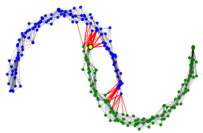
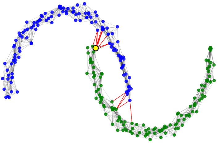
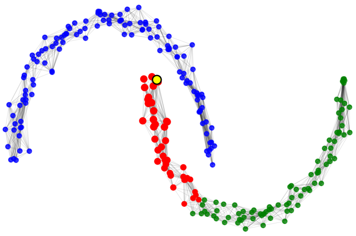
In this paper, we found that this reciprocity check with NN graph is insufficient to address the noisy edge problem, since the reciprocity check considers only reciprocal relationships between two edges. Since the reciprocity check and -NN constraints do not fully exploit all information from each other, we address the problem with full consideration of relationships between all edges in a clique where we can conservatively reach a consensus (Fig. 1). To realize this, we efficiently employ a fully connected C-CRF, when denoising the noisy NN graph in offline time.
Conditional Random Field (CRF) has been extensively studied [17], and Continuous CRF (C-CRF) [18] was proposed for regression tasks such as depth estimation, image denoising and metric learning for person re-ID [19, 20, 21]. Departing to these applications, our approach targets to refine similarities between each of database images that are robust to noisy edges for improving a diffusion performance in offline time.
Main contributions are summarized as follows:
-
•
We introduce a C-CRF based refinement method for noisy NN graphs that serves as a pre-processing module to enhance visual re-ranking.
-
•
Our approach utilizes a statistical distance metric to ensure robust distance measurement and employs cliques for cost-effective denoising.
-
•
We show that our method significantly enhances existing visual re-ranking methods in landmark retrieval and person re-identification, confirming its role as a complementary tool.
2 Visual re-ranking with NN graph
In this section, we summarize the diffusion process to show how the NN-graph can be applied for visual re-ranking. The diffusion process in visual re-ranking constructs revised similarity considering manifold from initial similarity computed from all images in the database. Generally, this process constructs an undirected graph structure from the affinity matrix, which is defined using the pairwise similarity between images, and performs diffusion on this graph using a random walk formulation [6, 12].
We define a database as a set of image descriptors, where each denotes a descriptor of image with dimensionality ; . We define the affinity matrix , , following the reciprocity check with a local constraint by considering nearest neighbors [6], where each element is obtained by:
| (1) |
| (2) |
where the similarity function is positive and has zero self-similarity, and denotes -NN of . Intuitively, equals to if , are the nearest neighbors of each other, and zero otherwise.
The degree matrix is a diagonal matrix with the row-wise sum of . It is used to symmetrically normalize as: . After the matrix computation, starting from an arbitrary vector that represents the initial similarity of a given query , the diffusion is performed until its state converges with a random walk iteration:
| (3) |
Zhou et al. [7] shows this iteration converges to a closed-form solution when assuming :
| (4) |
In the conventional diffusion process, the values in contain the refined similarity of the given query . Generally, the initial state represents the similarities between the query and the corresponding nearest neighbors as:
| (5) |
In this paper, we propose a novel, denoising approach for the initial affinity matrix to reduce the noisy edges.
3 Approach
Diffusion methods [6, 12] for image retrieval adopted a simple approach of using the reciprocity check (Eq. 2) with -NN of each database image to ameliorate noisy edges whose vertices are not positive, i.e., similar images. We, however, found that the reciprocity check is limited to handling noise, since identifying the noisy edge is based on the consensus of only two nodes of an edge, resulting incorrect identification of noise edges.
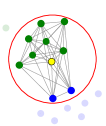
While this noisy edge problem was not seriously treated in diffusion approaches for image retrieval, we tackle the noisy edge problem by considering all neighbors from each image in a well-connected subgraph where we can robustly detect noisy edges. Specifically, we realize our goal by using C-CRF on subgraphs, i.e., cliques, with our proposed weight function (illustrated in Fig. 2).

3.1 C-CRF on clique
Our goal is to refine initial similarities of NN graph that are commonly set by top- similarities of each database image. For computational efficiency and effective noise handling, we utilize the concept of cliques and apply C-CRF into each of cliques. Specifically, we choose a clique, a complete subgraph, where we can have ample information such that we can identify noisy edges. On top of that, using the clique has computational benefits in running CRFs (Sec. 3.2).
We suppose that the whole database size is and a clique of a pivot image is , where a set of nodes (images) is composed of nearest neighbors from the pivot image by a specified clique size , and is a set of edges that makes the clique , i.e., a complete subgraph. Given a clique , its set of initial similarities can be computed by the cosine similarity or Euclidean distance. For simplicity, we express as . The set is fed as input to C-CRF and is defined: with the given initial similarity on clique . C-CRF computes a set of refined similarities defined as , which has elements with refined similarity .
C-CRF on each clique is represented by a conditional probability as follows:
| (6) |
where is a normalization constant. The corresponding energy function, , can be defined by linearly combining a unary potential and a pairwise potential with positive scalars and , as follows:
| (7) |
The unary potential, , intends to follow the initial similarity . To consider inter-image relationships, the pairwise potential is defined as:
| (8) |
where and are feature vectors of node and node , respectively, and weight is introduced to measure a conformity between node and node in the feature space and similarity-based distribution. Intuitively, the pairwise potential encourages that as a higher weight of node and node , the closer refined similarity values between and . These potentials are designed to reach a consensus from all the nodes on a clique for refining the initial similarities.
While we perform C-CRF on cliques to be robust against noisy edges, we further found that, in challenging datasets, a high number of noisy edges can exist even in the clique, deteriorating the similarity refinement process through C-CRFs. As a result, we design the weight function to be robust even in this extreme case by utilizing a statistical distance considering a similarity-based distribution in the clique.
More specifically, our probability mass function (PMF) in terms of a node is defined by -normalization within a clique of a pivot node , followed by a softmax as:
| (9) |
where is a -normalized in terms of .
We assume that two nodes have statistically similar distributions, if those two nodes are close to each other based on this PMF. In other words, PMF of a node is designed to serve as a descriptor of the node and, in this sense, we call it Similarity-Based Distribution (SBD). We then employ Jeffreys Divergence (J-Divergence) [22] symmetrizing Kullback-Leibler divergence for calculating the statistical distance between two distributions, as follows:
| (10) |
where each of is a vector that has bins for all the other nodes in .
Finally, our weight function can be characterized with a Gaussian kernel of the Euclidean distance between two feature vectors and , and our statistical distance:
| (11) |
where hyper parameters, and , adjust the degree of nearness. In the Gaussian kernel of our weight function, we call the first term as Euclidean Distance (ED) and the second term as Statistical Distance (SD). In an extreme case of calculating a weight between a node and its hard negative, our SD can identify the hard negative better than ED. This is because SD sees all the other nodes in the clique, some of which are properly represented in the feature space, even while the hard negative is not.
Multivariate Gaussian form. For ease of explanation, we now use a matrix notation within a clique of a specified size such as a weight matrix, , whose element corresponds to . From now on, we also treat as a matrix that is composed of elements for the sake of simple explanation. A variant [23] of the C-CRF method simply represents Eq. 6 into a multivariate Gaussian form, as follows:
| (12) |
The covariance matrix and mean is then defined as:
| (13) |
where , , and is the degree matrix of .
Inference. We can simply find that maximizes the conditional probability by following the Gaussian property:
| (14) |
We then repeat to calculate the solution for the whole database images by setting each database image to a pivot image . We can also employ a conjugate gradient (CG) method [24] to calculate the approximated solution of the inverse problem for computational efficiency. A constraint for CG is satisfied because the covariance matrix is symmetric and positive semi-definite.
Affinity matrix of denoised similarities. Existing diffusion methods [6, 12] employed the reciprocity check over -NN lists for constructing an affinity matrix due to noises and outliers. On the other hand, our denoised similarities of do not have much of noises and outliers. Thus we can instead use a simple symmetric affinity from the NN graph of our denoised similarities as . Afterward, we follow steps of each of diffusion methods with the denoised, symmetric affinity matrix to perform image retrieval.
3.2 Offline complexity
Thanks to the strategic use of cliques, we achieve significant computational efficiency in our C-CRF based denoising process. We outline the computational complexity by detailing each component involved in the process. For the inference stage of a pivot point, we perform three kinds of operations, such as -NN for finding its clique, computing the weight matrix within the clique and calculating the solution for similarity inference. The optimal -NN search takes with a whole database size , and it can be accelerated by using some approximated methods [25] if is sufficiently large. Computing the weight matrix costs with the specified clique size since J-Divergence (Eq. 10) takes and lower order terms, such as Euclidean distance, -normalization and softmax, are disregarded. For similarity inference, it takes with a specified number of iterations, , for the conjugate gradient method [24]. Note that complexities of these operations are bounded to the fixed clique size and the whole complexity for one pivot then becomes a constant time. We perform the same C-CRF refinement for each database image, but this can be parallelized and accelerated by using GPUs and CPUs.
4 Experiments
In this section, we explore the application of our denoising approach to two distinct but related tasks: landmark retrieval and person re-identification (re-ID). Both tasks benefit from robust image retrieval techniques, making them ideal for demonstrating the versatility of our method.
4.1 Experimental setup
Datasets and features. We conduct our experiments using challenging datasets: Oxford and Paris [26] for landmark retrieval, and DukeMTMC-reID [27] for re-ID. Oxford and Paris have three kinds of evaluation protocols, i.e., Easy, Medium, and Hard. Specifically, Oxford contains images and queries that represent particular Oxford landmarks and Paris consists of images and queries related to particular Paris landmarks. DukeMTMC-reID has 16,522 images with 702 identities for training, 2,228 images with 702 ids for query and 17,661 images for the gallery.
We employ GeM networks [28] of ResNet and VGG versions for landmark retrieval, which are seminal and easy to reproduce in a publicly available author’s implementation111https://github.com/filipradenovic/cnnimageretrieval-pytorch. For re-ID, we leverage ResNet-50 [29], which is publicly available in a repository222https://github.com/layumi/Person_reID_baseline_pytorch, for the baseline network.
Parameter setup. We simply fix C-CRF parameters , to , , respectively, for all the following experiments. Parameters , of the Gaussian kernel are set to , for VGG and , for ResNet. We empirically choose clique sizes of , and for Oxford, Paris and DukeMTMC-reID datasets, respectively due to the diverse distributions over different datasets. For other baseline methods, we mainly follow the same parameters of each method.
4.2 Results
| Method | Easy | Medium | Hard | |
|---|---|---|---|---|
| ResNet | NN-Search | 84.2 | 65.4 | 40.1 |
| NNS + AQE | 81.9 | 67.1 | 42.7 | |
| EGT | 81.8 | 65.4 | 42.5 | |
| + Ours | 85.5(+3.7) | 73.2(+7.8) | 50.8(+8.3) | |
| Online diffusion | 84.4 | 67.0 | 37.9 | |
| + Ours | 91.5(+7.1) | 73.7(+6.3) | 45.3(+7.4) | |
| Offline adiffusion | 88.2 | 69.9 | 41.1 | |
| + Ours | 92.4(+4.2) | 76.1(+6.2) | 50.3(+9.2) | |
| VGG | NN-Search | 79.4 | 60.9 | 32. |
| NNS + AQE | 86.3 | 69.1 | 41.1 | |
| EGT | 88.3 | 71.6 | 44.9 | |
| + Ours | 87.5(-0.8) | 72.4(+0.8) | 46.7(+1.8) | |
| Online diffusion | 83.2 | 67.4 | 39.9 | |
| + Ours | 88.4(+5.2) | 71.4(+4.0) | 42.6(+2.7) | |
| Offline diffusion | 87.2 | 70.4 | 42.0 | |
| + Ours | 90.0(+2.8) | 73.1(+2.7) | 45.0(+3.0) |
| Method | Easy | Medium | Hard | |
|---|---|---|---|---|
| ResNet | NN-Search | 91.6 | 76.7 | 55.2 |
| NNS + AQE | 93.6 | 82.3 | 63.9 | |
| EGT | 92.8 | 82.7 | 68.6 | |
| + Ours | 92.7(-0.1) | 83.3(+0.6) | 69.6(+1.0) | |
| Online diffusion | 93.7 | 88.5 | 78.3 | |
| + Ours | 95.0(+2.3) | 91.0(+2.5) | 80.8(+2.5) | |
| Offline adiffusion | 94.2 | 87.9 | 77.6 | |
| + Ours | 95.1(+0.9) | 89.3(+1.4) | 78.7(+1.1) | |
| VGG | NN-Search | 86.8 | 69.3 | 44.2 |
| NNS + AQE | 91.0 | 75.4 | 52.7 | |
| EGT | 92.3 | 81.2 | 64.7 | |
| + Ours | 92.5(+0.2) | 83.1(+1.9) | 69.3(+4.6) | |
| Online diffusion | 92.7 | 85.9 | 74.2 | |
| + Ours | 94.7(+2.0) | 89.1(+3.2) | 78.2(+4.0) | |
| Offline diffusion | 92.2 | 84.1 | 72.3 | |
| + Ours | 93.3(+1.1) | 85.4(+1.3) | 73.2(+0.9) |
| Method | Rank 1 | mAP |
|---|---|---|
| NN-Search | 64.6 | 43.6 |
| k-reciprocal | 69.3 | 60.7 |
| EGT | 64.5 | 47.5 |
| + Ours | 64.6(+0.1) | 48.2(+0.7) |
| Online diffusion | 68.9 | 54.9 |
| + Ours | 70.7(+1.8) | 62.4(+7.5) |
| Offline diffusion | 68.6 | 55.0 |
| + Ours | 70.8(+2.2) | 62.2(+7.2) |
Complementarity Analysis. For validating the denoising quality, we exploit three re-ranking methods, i.e., online diffusion [6], offline diffusion [12], and Explore-Exploit Graph Traversal (EGT) [10]. Tables 1, 2, 3 show performance changes when our method is integrated with other re-ranking methods. Other tested method include Average Query Expansion (AQE) [4] on Oxford and Paris datasets, and k-reciprocal [30] for re-ID setting. In the comprehensive settings analyzed, our method predominantly demonstrated enhancements, with degradation occurring in only two cases, highlighting the high quality of our denoising approach. Overall, the average improvements with our method are 4.6 mAP for Oxford, 1.7 mAP for Paris and 3.3 mAP for DukeMTMC-reID. These results are mainly acquired thanks to our C-CRF based denoising.
| w/ ED | w/ SD | Offline diffusion | Online diffusion | |||
|---|---|---|---|---|---|---|
| Oxford | Paris | Oxford | Paris | |||
| ResNet | 69.9 | 87.9 | 67.0 | 88.5 | ||
| ✓ | 75.5 | 89.2 | 71.4 | 89.8 | ||
| ✓ | 75.9 | 89.3 | 73.0 | 91.0 | ||
| ✓ | ✓ | 76.1 | 89.3 | 73.7 | 91.0 | |
| VGG | 70.4 | 84.1 | 67.4 | 85.9 | ||
| ✓ | 70.9 | 84.9 | 67.8 | 86.2 | ||
| ✓ | 72.7 | 85.3 | 71.0 | 88.9 | ||
| ✓ | ✓ | 73.1 | 85.4 | 71.4 | 89.1 | |
Ablation study. We conduct ablation experiments for each term of the weight function of the C-CRF on both of online diffusion [6] and offline diffusion [12]. The experiments are conducted with the Medium protocol of Oxford and Paris, since the Medium protocol consisting of both of Easy and Hard images that can represent an overall quality of retrieval results. Table 4 displays performances with different weight terms on each network for feature extraction. As shown in the ablation study, we see that using both terms of the Euclidean Distance (ED) of CNN-based features and the Statistical Distance (SD) of similarity-based distributions for the weight function yields the best performance. We then use our C-CRF with ED and SD in the rest of experiments.
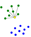
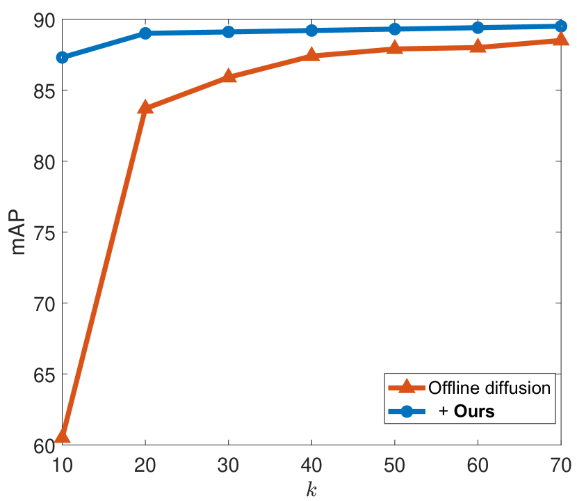
In Figure 3, we additionally experiment with measuring performance effect on varying parameters since a sparsity of the -NN graph is determined from the , and the sparsity affects the online time complexity; specifically, high density gives rise to high diffusion complexity. In the same vein, our resulting graph outperforms the reciprocal-NN graph with a more significant gap for smaller k (than 50), and this means we can reduce the online time complexity with less degradation of the retrieval quality. Furthermore, diffusion-based methods are known to be sensitive to the choice of parameters [31]. Our approach helps to mitigate the sensitivity to the important parameter .
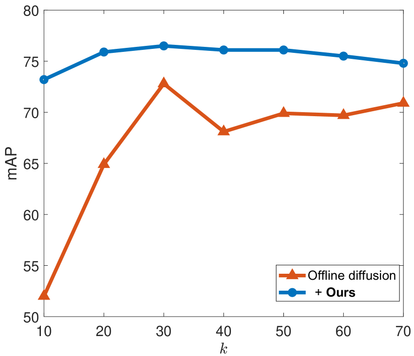
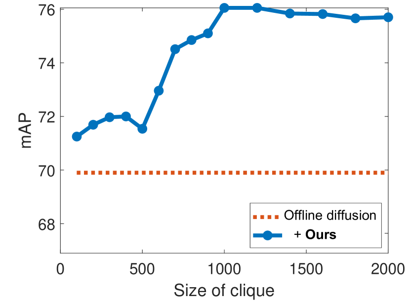
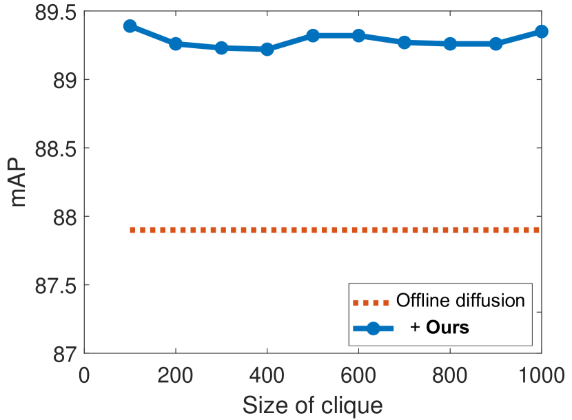
In Figure 4, the mAP performances are shown with varying clique sizes. The ablation study analyzes the performance according to the clique size, demonstrating robust results over a wide range of clique sizes compared to the baseline. We choose appropriate clique sizes based on this study, even though our method is robust to varying clique sizes in a wide range when compared to baseline.
0pt
R:\nth94
0pt
R:\nth78
0pt
R:\nth74
0pt
R:\nth5
0pt
R:\nth47
0pt
R:\nth48
0pt
R:\nth49
0pt
R:\nth50
4.3 Qualitative results
To see how much our C-CRF adjusts initial similarities, Figure 5 demonstrates ranking changes among offline database images with ResNet. We can see the affirmative ranking changes after applying our C-CRF refinement. For example, rankings of upper R:\nth5 and lower R:\nth47 images, which are positive to the pivot image , are pulled up, while rankings of lower R:\nth48, R:\nth49 and R:\nth50 negative images are pushed away.
Note that if an image rank is greater than value, e.g., 50 for the test of online and offline diffusion, for locally constrained affinity, the image will be filtered out from the affinity. As a result, the upper negative images of Figure 5 are cut out, while constructing a locally constrained affinity with our refined similarities, since the rankings are changed from I:\nth47, I:\nth48 and I:\nth49 to R:\nth94, R:\nth78 and R:\nth74. Figure 6 shows that our SD can catch hard positives better than ED in the example. Our SD tends to give relatively higher weights for positive images than weights for negative images, when compared with those of ED.

0pt
G-SD:0.65
0pt
G-SD:0.68
0pt
G-SD:0.45
0pt
G-SD:0.35
0pt
G-SD:0.37
0pt
G-SD:0.27
5 Conclusion
In this study, we introduced a C-CRF based refinement method for denoising NN graph, which is crucial for visual re-ranking. By leveraging cliques, this method enhances computational efficiency while ensuring robust distance measurements through statistical distance metrics for C-CRF. Our approach significantly improves performance in landmark retrieval and person re-identification tasks, demonstrating its effectiveness as a pre-processing tool for enhancing visual re-ranking accuracy.
References
- [1] O. Siméoni, Y. Avrithis, O. Chum, Local features and visual words emerge in activations, CoRR abs/1905.06358. arXiv:1905.06358.
- [2] H. Noh, A. Araujo, J. Sim, T. Weyand, B. Han, Large-scale image retrieval with attentive deep local features, in: IEEE International Conference on Computer Vision, ICCV 2017, 2017.
- [3] J. Kim, S. Yoon, Regional attention based deep feature for image retrieval, in: British Machine Vision Conference 2018, 2018, p. 209.
- [4] O. Chum, J. Philbin, J. Sivic, M. Isard, A. Zisserman, Total recall: Automatic query expansion with a generative feature model for object retrieval, in: IEEE International Conference on Computer Vision, ICCV 2007, 2007.
- [5] J. Philbin, O. Chum, M. Isard, J. Sivic, A. Zisserman, Object retrieval with large vocabularies and fast spatial matching, in: Proceedings of the IEEE Conference on Computer Vision and Pattern Recognition, 2007.
- [6] A. Iscen, G. Tolias, Y. Avrithis, T. Furon, O. Chum, Efficient diffusion on region manifolds: Recovering small objects with compact CNN representations, in: IEEE Conference on Computer Vision and Pattern Recognition, CVPR 2017, 2017.
- [7] D. Zhou, J. Weston, A. Gretton, O. Bousquet, B. Schölkopf, Ranking on data manifolds, in: Advances in Neural Information Processing Systems, 2003.
- [8] M. Donoser, H. Bischof, Diffusion processes for retrieval revisited, in: IEEE Conference on Computer Vision and Pattern Recognition 2013, 2013.
- [9] S. Bai, X. Bai, Q. Tian, L. J. Latecki, Regularized diffusion process on bidirectional context for object retrieval, IEEE Trans. Pattern Anal. Mach. Intell. 41 (5) (2019) 1213–1226.
- [10] C. Chang, G. Yu, C. Liu, M. Volkovs, Explore-exploit graph traversal for image retrieval, in: Proceedings of the IEEE Conference on Computer Vision and Pattern Recognition, 2019, pp. 9423–9431.
- [11] S. Qi, Y. Luo, Object retrieval with image graph traversal-based re-ranking, Sig. Proc.: Image Comm. 41 (2016) 101–114.
- [12] F. Yang, R. Hinami, Y. Matsui, S. Ly, S. Satoh, Efficient image retrieval via decoupling diffusion into online and offline processing, CoRR abs/1811.10907. arXiv:1811.10907.
- [13] J. Ouyang, H. Wu, M. Wang, W. Zhou, H. Li, Contextual similarity aggregation with self-attention for visual re-ranking, Advances in Neural Information Processing Systems 34 (2021) 3135–3148.
- [14] S. Shao, K. Chen, A. Karpur, Q. Cui, A. Araujo, B. Cao, Global features are all you need for image retrieval and reranking, in: Proceedings of the IEEE/CVF International Conference on Computer Vision, 2023, pp. 11036–11046.
- [15] G. An, J.-h. Seon, I. An, Y. Huo, S.-E. Yoon, Topological ransac for instance verification and retrieval without fine-tuning, Advances in Neural Information Processing Systems 36.
- [16] X. Yang, S. Köknar-Tezel, L. J. Latecki, Locally constrained diffusion process on locally densified distance spaces with applications to shape retrieval, in: IEEE Computer Society Conference on Computer Vision and Pattern Recognition (CVPR 2009), 2009.
- [17] C. Sutton, A. McCallum, An introduction to conditional random fields for relational learning, in: L. Getoor, B. Taskar (Eds.), Introduction to Statistical Relational Learning, MIT Press, 2006, to appear.
- [18] T. Qin, T. Liu, X. Zhang, D. Wang, H. Li, Global ranking using continuous conditional random fields, in: Advances in Neural Information Processing Systems 2008, 2008.
- [19] F. Liu, C. Shen, G. Lin, Deep convolutional neural fields for depth estimation from a single image, in: IEEE Conference on Computer Vision and Pattern Recognition, CVPR 2015, 2015.
- [20] K. Ristovski, V. Radosavljevic, S. Vucetic, Z. Obradovic, Continuous conditional random fields for efficient regression in large fully connected graphs, in: AAAI Conference on Artificial Intelligence, 2013.
- [21] D. Chen, D. Xu, H. Li, N. Sebe, X. Wang, Group consistent similarity learning via deep CRF for person re-identification, in: IEEE Conference on Computer Vision and Pattern Recognition, CVPR 2018, 2018.
- [22] H. Jeffreys, Scientific inference, Cambridge [Eng.] : Cambridge University Press, 1973.
- [23] V. Radosavljevic, S. Vucetic, Z. Obradovic, Continuous conditional random fields for regression in remote sensing, in: ECAI 2010 - 19th European Conference on Artificial Intelligence, Lisbon, Portugal, August 16-20, 2010, Proceedings, 2010, pp. 809–814.
- [24] J. R. Shewchuk, et al., An introduction to the conjugate gradient method without the agonizing pain (1994).
- [25] J. Johnson, M. Douze, H. Jégou, Billion-scale similarity search with gpus, IEEE Transactions on Big Data 7 (3) (2019) 535–547.
- [26] F. Radenovic, A. Iscen, G. Tolias, Y. Avrithis, O. Chum, Revisiting oxford and paris: Large-scale image retrieval benchmarking, in: IEEE Conference on Computer Vision and Pattern Recognition, CVPR 2018, 2018.
- [27] Z. Zheng, L. Zheng, Y. Yang, Unlabeled samples generated by gan improve the person re-identification baseline in vitro, in: Proceedings of the IEEE International Conference on Computer Vision, 2017, pp. 3754–3762.
- [28] F. Radenovic, G. Tolias, O. Chum, Fine-tuning CNN image retrieval with no human annotation, IEEE Trans. Pattern Anal. Mach. Intell. 41 (7).
- [29] Z. Zheng, X. Yang, Z. Yu, L. Zheng, Y. Yang, J. Kautz, Joint discriminative and generative learning for person re-identification, IEEE Conference on Computer Vision and Pattern Recognition (CVPR).
- [30] Z. Zhong, L. Zheng, D. Cao, S. Li, Re-ranking person re-identification with k-reciprocal encoding, in: Proceedings of the IEEE Conference on Computer Vision and Pattern Recognition, 2017, pp. 1318–1327.
- [31] F. Magliani, L. Sani, S. Cagnoni, A. Prati, Genetic algorithms for the optimization of diffusion parameters in content-based image retrieval, in: Proceedings of the 13th International Conference on Distributed Smart Cameras, 2019, pp. 1–6.