Information-Theoretic Generative Clustering of Documents

Abstract

We present generative clustering (GC) for clustering a set of documents, $\mathrm{X}$, by using texts $\mathrm{Y}$ generated by large language models (LLMs) instead of by clustering the original documents $\mathrm{X}$. Because LLMs provide probability distributions, the similarity between two documents can be rigorously defined in an information-theoretic manner by the KL divergence. We also propose a natural, novel clustering algorithm by using importance sampling. We show that GC achieves the state-of-the-art performance, outperforming any previous clustering method often by a large margin. Furthermore, we show an application to generative document retrieval in which documents are indexed via hierarchical clustering and our method improves the retrieval accuracy.

Code — https://github.com/kduxin/lmgc

1 Introduction

Document clustering has long been a foundational problem in data science. Traditionally, every document $x\in\mathrm{X}$ is first translated into some computational representation $y\in\mathbb{R}^{n}$: in the 90s, as a bag-of-words vector, and more recently, by using BERT (Devlin et al. 2019). A clustering algorithm, typically $k$-means, is then applied.

While large language models (LLMs) have been applied to diverse tasks, their use in basic document clustering remains underexplored. Traditionally, the translation of a document $x$ into a representation $y$ was considered a straightforward vectorization step. However, texts are often sparse, with much that is unsaid and based on implicit knowledge. By using LLMs, like GPT-4 (OpenAI 2023), to generate $y$ by complementing this missing knowledge, could the content of $x$ be better explicated and yield a better clustering result?

In this paper we explore the effect of using an LLM to rephrase each document $x\in\mathrm{X}$. Previously, the term “generative clustering” was used to refer to approaches where document vectors appear to be “generated” from clusters (Zhong and Ghosh 2005; Yang et al. 2022). In this paper, however, “generative” refers to the use of a generative LLM.

The use of an LLM to translate $x$ into $y$ has the further benefit of opening the possibility to mathematically formulate the information underlying $x$ more accurately. Previously, when clustering a set of documents $x$ directly, not much could be done statistically, given the bound by a finite number of words and the lack of underlying knowledge. When using a simple representation such as bag of words, document vectors are generated by a Gaussian distribution for each cluster, thus reducing the clustering into a simple $k$-means problem. On the other hand, if we incorporate a set of $y$ produced by an LLM, the clustering problem can be rigorously formulated using information-theory, according to the probabilistic pairing information of $x\leftrightarrow y$.

Specifically, $y$ can be defined over the infinite set $\mathcal{Y}$ of all possible word sequences of unlimited length. Each document is represented by a probability distribution over generated texts in $\mathcal{Y}$, denoted as $p(Y=y|X=x)$. The dissimilarity between documents is quantified using the KL divergence between their respective distributions over the generated texts. Clustering then is performed by grouping documents based on the similarity of these distributions.

In this paper, we show that large improvements often result for plain document clustering in this new generative clustering setting. This suggests that the quantity of knowledge underlying a text is indeed large, and that such knowledge can be inferred using generative LLMs.

This gain is already important even under the typical Gaussian assumption that is often adopted when clustering $X$ directly. Clustering of $Y$, however, can go much further. For generative clustering, the Gaussian assumption can be replaced by a more natural distribution through importance sampling. We empirically show that our proposed method achieved consistent improvement on four document-clustering datasets, often with large margins.

The proposed method’s possible applications are vast, entailing all problems that involve clustering. Here, we investigate the generative document retrieval (GDR) (Tay et al. 2022; Wang et al. 2022). In GDR, documents are indexed using a prefix code acquired via hierarchical clustering. We show that, on the MS Marco Lite dataset, GDR with the proposed generative clustering (GC) method achieved up to 36% improvement in the retrieval accuracy.

2 Related Works

2.1 Document Clustering

Document clustering is a fundamental unsupervised learning task with broad applications. Traditional methods depend on document representations like bag of words (BoW), tf-idf, and topic models such as latent Dirichlet allocation (LDA) (Blei, Ng, and Jordan 2003).

Recent advancements in text representation learning have significantly improved clustering performance. Techniques like continuous bag of words (CBoW) (Mikolov et al. 2013) generate low-dimensional word vectors, which can be averaged to form document vectors. Deep neural networks have further enhanced these embeddings by incorporating contextual information, as seen in models like ELMo (Peters et al. 2018), BERT (Devlin et al. 2019), and SentenceBERT (Reimers and Gurevych 2019).

These methods focus on encoding documents as dense vectors that capture similarities across texts. Studies have demonstrated the effectiveness of pretrained models for clustering (Subakti, Murfi, and Hariadi 2022; Guan et al. 2022), along with further improvements by using deep autoencoders and contrastive learning (Xie, Girshick, and Farhadi 2016; Guo et al. 2017).

However, these approaches may not fully capture deeper knowledge within texts, as BERT-like models are limited by their fixed vector outputs and cannot complete complex tasks. In contrast, generative models like GPT-4 (OpenAI 2023) can handle complex reasoning through autoregressive text generation (Kojima et al. 2022), though their use in clustering is still being explored.

Recent works have attempted to use generative LLMs for clustering, but these approaches lack a rigorous foundation. Viswanathan et al. (2023) explored the use of GPT models at several clustering stages, including document expansion before vector encoding, generation of clustering constraints, and correction of clustering results. Zhang, Wang, and Shang (2023) used LLMs to predict a document’s relative closeness to two others and performed clustering based on these triplet features. In contrast, our method formulates the clustering problem in a rigorous information-theoretic framework and leverages the LLM’s ability to precisely evaluate generation probabilities that were not used in these previous works.

2.2 Generative Language Models

Generative language models are those trained to predict and generate text autoregressively; they include both decoding-only models like GPT and encoder-decoder models like T5 (Raffel et al. 2020). While their architectures differ, both types of models function similarly, and a GPT model can be used in a manner similar to the use of T5.

T5 models are typically trained in a multi-task setting, with task-specific prefixes attached to input texts during training. In Sections 6 and 7, we explore a specific pre-trained T5 model called doc2query (Nogueira, Lin, and Epistemic 2019), which has been trained on various tasks, including query generation, title generation, and question answering.

2.3 Information-Theoretic Clustering

Information-theoretic clustering uses measures like the KL divergences or mutual information as optimization objectives (Dhillon, Mallela, and Modha 2003; Slonim and Tishby 2000). As described in Section 3, we aim to minimize the total KL divergence between documents and their cluster centroids, where the centroids are represented as distributions over the infinite set $\mathcal{Y}$.

This approach is effective for finite discrete distributions, such as word vocabularies, where the KL divergence can be computed exactly. In continuous spaces, however, KL divergence estimation requires density estimation, which involves assumptions about the data distribution and limits applicability. Many studies have tackled these challenges (Pérez-Cruz 2008; Wang, Kulkarni, and Verdú 2009; Nguyen, Wainwright, and Jordan 2010).

In our approach, $\mathcal{Y}$ is an infinite discrete space where the probability mass for each text can be evaluated exactly, though it remains challenging to manage this infinite space. We address this issue by using importance sampling (Kloek and Van Dijk 1978), as detailed in Section 5.

3 Generative Clustering of Documents

A clustering, in this work, is defined as a partition of documents $\mathrm{X}$ into $K$ clusters. Each document $x\in\mathrm{X}$ is associated with a conditional probability distribution $p(Y=y|x)$, which is defined for $y$ over the infinite set $\mathcal{Y}$ of all possible word sequences. $p(Y=y|x)$ measures the probability mass that a text $y$ is generated from a document $x$, and this value is calculated by using a generative language model with the following decomposition into word probabilities:

$$p(y|x)=p(\omega_{1}|x)\,p(\omega_{2}|x,\omega_{1})\ldots p(\omega_{l}|x,\omega_{1},\cdots,\omega_{l-1}),$$ (1)

where $\omega_{1},\omega_{2},\ldots,\omega_{l}$ are the words in the text $y$ and $l$ is the text’s length.

Each cluster $k$ ($k=1,2,\cdots,K$) is also associated with a distribution over $\mathcal{Y}$, denoted as $p(Y|k)$. We refer to $p(Y|k)$ as a cluster’s “centroid” in this paper.

The clustering objective is to jointly learn a cluster assignment function $f:\mathrm{X}\to\{1,2,\cdots,K\}$ and the cluster centroids $p(Y|k)$ while minimizing the total within-cluster distortion, as follows:

$$\min_{f,\{p(Y|k)\}_{k}}D =\sum_{x\in\mathrm{X}}d(x,f(x)),$$ (2)

$$\text{where}~{}d(x,k) =\mathrm{KL}\bigl{[}p(Y|x)\lVert p(Y|k)\bigr{]},$$ (3)

If $\mathcal{Y}$ were finite, this objective is no more than a special case of the Bregman hard clustering problem (Banerjee et al. 2005). Note that $k$-means is a special case, too. However, as mentioned at the beginning of this section, $\mathcal{Y}$ is infinite; therefore, we need to figure out how to calculate $p(Y|k)$. Unlike the document-specific distribution $p(Y|x)$, which is acquired easily via an LLM, $p(Y|k)$ is unknown. Moreover, we obviously need to determine how to calculate the KL divergence for $\forall x,k$.

The condition probability $p(Y|x)$ can be seen as a novel kind of document embedding for $x$. An embedding is a distribution over $\mathcal{Y}$, and is thus infinitely dimensional. By selecting a proper set of texts $\mathrm{Y}$, $p(Y|x)$ can be “materialized” as a vector, with each entry being $p(Y=y|x)$ for a text $y\in\mathrm{Y}$. However, the choice of $\mathrm{Y}$ is crucial, and how to use the vector for clustering is not straightforward. We answer these questions by proposing a novel clustering algorithm in Section 5.

4 A Conventional Baseline Using BERT

Conventional clustering methods can be interpreted as a baseline solution to the above problem, via approximating the KL divergence by using a BERT model (Devlin et al. 2019), for example, to embed the generated texts $Y$ into a low-dimensional vector space. In other words, each of $p(Y|x)$ and $p(Y|k)$ is a distribution over the vector space.

Then, the clustering problem specified by Eqs. (2-3) is solved by using a standard $k$-means algorithm and assuming the distributions $p(Y|x)$ and $p(Y|k)$ are both Gaussian. Here, Eq. (2) reduces to:

$$\min_{f,\{\mathbb{E}[p(Y|k)]\}_{k}}D=\sum_{x\in\mathrm{X}}\lVert\mathbb{E}[p(Y|x)]-\mathbb{E}[p(Y|f(x))\rVert^{2},$$ (4)

where $f(x)$ is the cluster that $x$ is assigned to, $\mathbb{E}$ represents the mean vector of a Gaussian distribution. $\mathbb{E}[p(Y|x)]$ is estimated by the center vector of texts sampled from $x$.

There are multiple methods to obtain $\mathbb{E}[p(Y|x)]$ and we consider two here. The first is to let $\mathbb{E}[p(Y|x)]=\text{BERT}(x)$, i.e., the document’s embedding. This method is equivalent to the most common clustering method and does not use the generative language model. In contrast, the second method uses the model by generating multiple texts for each document $x$ and letting $\mathbb{E}[p(Y|x)]$ be the mean vector of the generated texts’ embeddings. The mean vector is used because it is a maximum-likelihood estimator of $\mathbb{E}[p(Y|x)]$.

Unfortunately, such conventional solutions involve multiple concerns. It could be overly simplistic to assume that the generated texts are representable within the same vector space and that $p(Y|x)$ and $p(Y|k)$ follow Gaussian distributions. In fact, $p(Y|x)$ often exhibits multimodality when we use a BERT model to embed the generated texts. Furthermore, this solution uses a text embedding model in addition to the generative language model, and the possible inconsistency between these two models might degrade the clustering quality.

5 Generative Clustering
Using Importance Sampling

5.1 Two-Step Iteration Algorithm

Given the above concerns, we propose to perform generative clustering by using importance sampling over $\mathcal{Y}$.

First of all, we use the typical two-step iteration algorithm, as generally adopted in $k$-means. This is the common solution for all Bregman hard clustering problems (Banerjee et al. 2005), by repeating the following two steps:

1. Assign each document $x$ to its closest cluster by distance $d(x,k)$.

2. Update every cluster centroid to minimize the within-cluster total distance from the documents to the centroid.

We formally implement this as Algorithm 1. The $d(x,k)$ function is defined in the following subsection. The algorithm starts in line 1 by sampling a set of texts $\mathrm{Y}=\{y_{1},y_{2},\cdots,y_{J}\}$ from the LLM, as explained further in Section 5.3. Then, the algorithm computes two matrices, which both have rows corresponding to documents and columns corresponding to sampled texts in $\mathrm{Y}$. The first matrix (line 2) is the probability matrix of $\mathbf{P}_{ij}\equiv p(y_{i}|x_{i})$, acquired from the LLM. After a clipping procedure for $\mathbf{P}_{ij}$ (line 3, Section 5.5) and estimation of the proposal distribution $\phi(y_{j})$ (line 4, Section 5.3), the second matrix (lines 4,5) is acquired as regularized importance weights $\mathbf{W}$ such that $\mathbf{W}_{ij}\equiv(p(y_{j}|x_{i})/\phi(y_{j}))^{\alpha}$, where $\alpha$ is a hyperparameter explained in the following section. Next, the clustering algorithm, defined in lines 8-15, is called (line 6). After centroid initialization (line 9, Section 5.4), the two steps described above are repeated (lines 11 and 12-13, respectively).

Algorithm 1 is guaranteed to converge (to a local minimum), and we provide a proof in Appendix A.1 (Proposition 1).

Algorithm 1 Generative clustering of documents.

Input: Documents $\mathrm{X}$; a finetuned language model.
Parameters: Number of clusters, $K$; number of text samples, $J$; proposal distribution, $\phi$; regularization factor, $\alpha$.
Output: Cluster assignment function $f:\mathrm{X}\to\{1,2,\cdots,K\}$.

1:

Generate $\mathrm{Y}=\{y_{1},\cdots,y_{J}\}$ by i.i.d. sampling from the language model.

2:

Compute $\mathbf{P}_{ij}=p(y_{j}|x_{i})$ for any $x_{i}\in\mathrm{X}$ and $y_{j}\in\mathrm{Y}$ via the language model.

Eq.(1)

3:

Clip $\mathbf{P}_{ij}$ to avoid outlier values.

Eq.(11)

4:

For $y_{j}\in\mathrm{Y}$, estimate $\phi(y_{j})$.

Eq.(7)

5:

Compute the importance weight matrix
$\mathbf{W}_{ij}=(\mathbf{P}_{ij}/\phi(y_{j}))^{\alpha}$.

6:$f\leftarrow\textsc{Clustering}(\mathbf{P},\mathbf{W})$

7:

8:function Clustering($\mathbf{P},\mathbf{W}$)

9:     

Initialize cluster centroids $\mathbf{c}_{k}$ ($\forall k$) by randomly selecting a row of $\mathbf{W}$ and normalizing it.

Eq.(9)

10:     do

11:         

$f(x_{i})\leftarrow$ closest cluster to $x_{i}$, $\forall x_{i}\in\mathrm{X}$.

Eq.(5)

12:         

Update the centroid $\mathbf{c}_{k}$.

Eq.(10)

13:         

Compute the total distortion
$\sum_{x\in\mathrm{X}}\hat{d}(x,f(x))$.		Eq.(5)

14:     while the total distortion improves.

15:     return $f$

5.2 Distortion Function $d(x,k)$

The distortion function $d(x,k)$ was defined in Eq. (3) as the KL divergence between $p(Y|x)$ and $p(Y|k)$, but it is not computable because of the infinite $\mathcal{Y}$. Therefore, we apply the importance sampling (IS) technique (Kloek and Van Dijk 1978) to estimate $d$. IS is a statistical technique to estimate properties of a particular distribution from a different distribution $\phi$ called the proposal. The technique’s effectiveness is demonstrated by the following equality:

$$\mathbb{E}_{Y\sim p(Y|x)}\left[\log\frac{p(Y|x)}{p(Y|k)}\right]=\mathbb{E}_{Y\sim\phi}\left[\frac{p(Y|x)}{\phi(Y)}\log\frac{p(Y|x)}{p(Y|k)}\right],$$

where the left side is the KL divergence, and $\frac{p(Y|x)}{\phi(Y)}$ on the right side is called the importance weight. By using IS, the KL divergence for each document can be estimated efficiently by using samples generated from a shared $\phi$ (i.e., $\mathrm{Y}$ in line 1 of Algorithm 1) across all documents, instead of a separate distribution $p(Y|x)$ for each document.

A long-standing problem of IS-based estimators is the potentially large variance if the proposal $\phi$ is poorly selected and distant from the original distribution $p(Y|x)$. In addition to carefully selecting $\phi$, as detailed in Section 5.3, we adopt a regularized version of IS (RIS) (Korba and Portier 2022), which imposes an additional power function (with parameter $\alpha$) on the importance weights. Our estimator $\hat{d}$ based on RIS is defined as follows:

$$\hat{d}(x,k)\equiv\frac{1}{J}\sum_{\begin{subarray}{c}j=1\\ y_{j}\sim\phi(Y)\end{subarray}}^{J}\left(\frac{p(y_{j}|x)}{\phi(y_{j})}\right)^{\alpha}\log\frac{p(y_{j}|x)}{p(y_{j}|k)}.$$ (5)

Here, $\alpha\in[0,1]$ defines the strength of regularization. When $\alpha=1$, Eq. (5) converges to the true KL divergence value as $J\to\infty$; otherwise, Eq. (5) is biased, and smaller $\alpha$ leads to more bias. $\alpha$ plays a central role in the experimental section and is further discussed after that, in Section 8. In this paper, $\alpha$ was set to 0.25 for all experiments. Notably, there are other choices for importance weight regularization, e.g., Aouali et al. (2024).

Using the matrices defined in Section 5.1, this function $\hat{d}$ is rewritten as follows:

$$\hat{d}(x_{i},k)=\frac{1}{J}\sum_{j=1}^{J}\mathbf{W}_{ij}\log\frac{\mathbf{P}_{ij}}{\mathbf{c}_{k}(j)},$$ (6)

where $\mathbf{c}_{k}$ is a vector representing the cluster centroid $p(Y|k)$, as defined later in Eq. (8). The weight matrix $\mathbf{W}$ assigns importance to each text $y_{j}$, typically favoring texts with higher probabilities (e.g., shorter texts). Unlike the Euclidean distance, which treats all dimensions equally, the weight matrix $\mathbf{W}$ introduces a preference for specific dimensions (i.e., specific texts in $\mathrm{Y}$), enabling the algorithm to optimize an information-theoretic quantity.

5.3 Proposal Distribution $\phi(Y)$

The proposal distribution $\phi(Y)$ in Eq. (5) serves two functions: (1) construction of $\mathrm{Y}=[y_{1},\cdots,y_{J}]$ by sampling $y_{j}$ from $\phi$, and (2) estimation of the probability mass $\phi(y_{j})$ for any text $y_{j}\in\mathrm{Y}$.

The idea of tuning the proposal $\phi$ for better estimation of some quantity of a single distribution is not novel. In our setting, however, we must estimate $d(x,k)$ for all $x$ and $k$, i.e., for multiple distributions. Therefore, we must carefully choose $\phi$, instead of using some standard distribution.

In this paper, we choose the prior distribution $p(Y)$ as the proposal $\phi(Y)$, for two reasons. First, $p(Y)$ is close to $p(Y|x)$ for all $x\in\mathrm{X}$, thus minimizing the RIS sampler’s overall variance across all documents. Second, it allows for a straightforward sampling process:

(i)

Randomly select a document $x$ from $\mathrm{X}$ uniformly.

(ii)

Generate a text $y_{j}$ from $x$ by using the language model.

Here, the documents $\mathrm{X}$ are assumed to be i.i.d. samples from the prior distribution $p(X)$.

For estimating $p(y_{j})$, a basic approach is to average $p(y_{j}|x)$ across all $x\in\mathrm{X}$, which is equivalent to averaging the $j$-th column of matrix $\mathbf{P}$. However, we have found that the following estimator works better with Algorithm 1:

$$\phi(y_{j})=p(y_{j})\leftarrow\left(\frac{1}{|\mathrm{X}|}\sum_{x\in\mathrm{X}}p(y_{j}|x)^{2\alpha}\right)^{1/2\alpha},$$ (7)

where $\alpha$ is the regularization parameter in Eq. (5). This function in Eq. (7) represents the optimal case for minimal variance. The function’s theoretical background and approximation are discussed in Appendix A.3 (Proposition 3).

5.4 Estimation of Cluster Centroid $p(Y|k)$.

Each cluster is specified by its “centroid” $p(Y|k)$, which is a probability distribution defined over the infinite space $\mathcal{Y}$. In our algorithm, $p(Y|k)$ is represented as a vector,

$$\mathbf{c}_{k}=[p(y_{1}|k),\cdots,p(y_{J}|k)],$$ (8)

comprising the values of $p(Y|k)$ on $\mathrm{Y}$, which is a subset of the infinite $\mathcal{Y}$. The total probability on $\mathrm{Y}$ is denoted by $C_{k}=\sum_{j}p(y_{j}|k)\leq 1$. Here, $C_{k}$ is a hyperparameter to adjust the assignment preference for cluster $k$, as increasing $C_{k}$ would reduce the distance (i.e., the KL divergence) from any document to cluster $k$. Because we have no prior knowledge about each cluster, we set $C_{1}=C_{2}=\cdots=C_{K}=:C$ in this paper, meaning there is no preference among clusters. Furthermore, the order of the distances from a document to all cluster centroids is preserved under variation of $C$, and we thus set $C=1$ for simplicity.

For initialization, $\mathbf{c}_{k}$ is set to a random row of $\mathbf{W}$ and normalized to sum to 1. Let $i_{k}$ denote the selected row’s index. Then, every entry of $\mathbf{c}_{k}$ is initialized as follows:

$$\mathbf{c}_{k}(j)\leftarrow\mathbf{W}_{i_{k}j}/\sum_{j^{\prime}=1}^{J}\mathbf{W}_{i_{k}j^{\prime}}.$$ (9)

We also tried a more sophisticated initialization method by adapting the $k$-means++ strategy(Arthur and Vassilvitskii 2006). However, the results were not significantly different on the datasets we used. We present the results in Appendix B.1.

After the assignment step in each iteration, the cluster centroids are updated. For cluster $k$, the optimal centroid vector $\mathbf{c}_{k}^{*}$ that minimizes the within-cluster total distortion is parallel to the mean vector of the rows in $\mathbf{W}$ for the documents belonging to this cluster. That is, at each iteration, every cluster centroid is updated as follows:

$$\mathbf{c}_{k}(j)\leftarrow\mathbf{c}_{k}^{*}(j)=\frac{1}{Z}\sum_{x_{i}\in f^{-1}(k)}\mathbf{W}_{ij},$$ (10)

where $Z=\sum_{j=1}^{J}\mathbf{c}_{k}^{*}(j)$ is the normalization term. The optimality is shown in Appendix A.2 (Proposition 2).

5.5 Probability Clipping

Probability clipping is common in importance sampling (Wu et al. 2020) to stabilize the estimation procedure, by eliminating outlier values in $\mathbf{P}$. Outliers typically occur in $\mathbf{P}_{ij}$ when $y_{j}$ is generated from $x_{i}$, and they can be several magnitudes larger than other values in the same column, which destabilize KL divergence estimation. We use the following criterion to reset these outliers in the logarithm domain:

$$\log\mathbf{P}_{ij}=\begin{cases}\mu_{j}+5\sigma_{j}&\text{if}~{}\log\mathbf{P}_{ij}>\mu_{j}+5\sigma_{j},\\ \log\mathbf{P}_{ij}&\text{otherwise},\end{cases}$$ (11)

where $\mu_{j}$ and $\sigma_{j}$ are the mean and standard deviation of the $j$-th column of $\log\mathbf{P}_{ij}$. This clipping step can be seen as a further regularization of the importance weights (Aouali et al. 2024).

6 Evaluation of Generative Clustering

6.1 Data

We conducted an evaluation of our method using four document clustering datasets: R2, R5, AG News, and Yahoo! Answers, as summarized in Table 1.

Dataset	# documents	mean # words	# clusters
R2	6,397	92.4	2
R5	8,194	116.4	5
AG News	127,600	37.8	4
Yahoo! Answers	1,460,000	69.9	10

Table 1: Document clustering datasets used for clustering.

Method	R2			R5			AG News			Yahoo! Answers
	ACC	NMI	ARI	ACC	NMI	ARI	ACC	NMI	ARI	ACC	NMI	ARI
$k$-means clustering
Non-neural document embeddings
Bag of words	65.0	3.3	5.9	40.1	20.0	16.1	29.4	1.68	0.7	15.2	3.1	1.0
tf-idf	77.7	40.2	31.1	48.6	33.2	18.6	43.0	15.9	15.5	18.9	6.0	2.5
LDA (Blei, Ng, and Jordan 2003)	85.3	49.9	48.5	61.7	40.4	37.2	45.1	28.4	22.2	21.8	10.0	4.5
[0.5pt/1pt]            BERT/SBERT document embeddings (different pretrained models)
Bert (base, uncased)	75.6	31.1	28.1	58.2	27.3	35.0	59.9	38.2	30.9	20.9	9.4	4.5
Bert-base-nli-mean-tokens	86.7	49.6	53.7	57.1	36.3	36.7	64.1	29.8	28.2	31.9	15.1	10.7
All-minilm-l12-v2	86.9	54.3	54.5	76.7	65.6	58.6	74.4	56.7	55.5	58.2	42.8	34.8
All-mpnet-base-v2	90.3	61.7	65.0	73.2	68.9	58.5	69.2	55.0	52.0	56.7	39.8	32.4
All-distilroberta-v1	92.0	65.6	70.5	69.7	65.2	62.4	67.0	56.1	51.9	57.5	42.6	34.2
[0.5pt/1pt]          Doc2query-based document embeddings
Doc2Query encoder	74.2	32.5	24.8	48.6	24.2	18.7	38.1	8.4	7.6	16.5	4.0	1.5
Doc2Query log-prob. $\mathbf{P}$	86.1	51.5	52.3	56.2	54.1	43.9	74.8	53.2	52.1	43.0	29.6	20.7
Other non-$k$-means clustering methods
GSDMM$\dagger$ (Yin and Wang 2014)	74.5	62.3	45.3	57.6	59.5	44.5	43.5	42.5	30.4	49.6	36.1	34.2
DEC$\dagger$ (Xie, Girshick, and Farhadi 2016)	76.0	37.4	36.9	37.9	22.2	18.5	47.0	12.4	11.5	14.2	1.2	1.1
IDEC$\dagger$ (Guo et al. 2017)	77.7	32.3	31.5	46.1	34.8	29.5	63.5	29.5	29.4	22.0	10.3	9.0
STC$\dagger$ (Xu et al. 2017)	77.9	35.7	36.5	57.1	40.8	37.5	64.6	39.2	38.8	37.7	23.6	21.4
DFTC$\dagger$ (Guan et al. 2022)	84.7	50.4	49.0	69.6	61.5	61.5	82.1	60.3	60.0	51.1	35.0	34.4
Generative clustering (ours)
GC ($\alpha=0.25$)	96.1	77.8	84.9	79.1	71.5	69.1	85.9	64.2	67.2	60.7	43.7	35.5
	(0.0)	(0.1)	(0.1)	(2.9)	(2.1)	(2.9)	(0.6)	(0.8)	(1.2)	(0.7)	(0.2)	(0.3)
[0.5pt/1pt]            Ablated versions
- $\alpha=1$ (unbiased KL estimation)	78.0	25.8	33.4	57.3	31.1	33.7	55.6	22.9	22.0	34.5	18.7	11.0
- Naïve $p(Y)$ estimator	95.9	77.1	84.2	79.3	71.1	68.5	85.0	63.2	65.5	60.5	43.4	35.6
- No probability clipping	95.1	73.2	81.2	76.4	65.6	63.0	80.6	60.7	59.4	57.5	42.3	33.7

Table 2: Clustering performance of various methods (rows) on four document datasets (columns). Methods marked with $\dagger$ in the first column were taken from Guan et al. (2022). The values in parentheses are standard deviations across 100 repeated experiments. The best score in each column is in bold and the second best is underlined.

R2 and R5 are subsets of Reuters-21587 and respectively contain documents from the largest two (earn, acq) and largest five (also crude, trade, money-fx) topics, following Guan et al. (2022). For AG News (Gulli 2005), we used the version provided by Zhang, Zhao, and LeCun (2015). Yahoo! Answers is a more challenging dataset with more documents and clusters.

For R2 and R5, we discarded documents tagged ambiguously with multiple topics. For AG News and Yahoo! Answers, we merged the training and test splits, as our method is unsupervised.

6.2 Evaluation Metrics & Settings

Following previous works (Guan et al. 2022; Zhou et al. 2022), we evaluated clustering methods by using three metrics:

Accuracy (ACC):

The percentage of correct cluster assignments, accounting for label permutations by maximizing the accuracy over all permutations with the Jonker-Volgenant algorithm (implemented in Python via

scipy.optimize.linear_sum_assignment).

A measure of the mutual information between true and predicted labels, normalized by the geometric mean of their Shannon entropies (Vinh, Epps, and Bailey 2010).

A variant of the Rand index that adjusts for random labeling and reduces the sensitivity to the number of clusters (Hubert and Arabie 1985).

Clustering algorithms are sensitive to initialization and affected by randomness. To mitigate this, we performed model selection by running each method 10 times with different seeds and selecting the run with the lowest total distortion. We repeated this process 100 times, and report the mean performance of the selected runs. For $k$-means, the distortion is the sum of the squared distances from points to their centroids. For our method, the distortion is $\sum_{x\in\mathrm{X}}\hat{d}(x,f(x))$, where $\hat{d}$ is defined in Eq. (5) and $f$ is the cluster assignment function. This model selection step uses no label information and is standard in practice.

For the language model, we used the pretrained doc2query model all-with_prefix-t5-base-v1. This model, trained on multiple tasks, attaches a task-specific prefix to each document. We used the general prefix “text2query:” to generate $\mathrm{Y}$, and we evaluated the generation probabilities from $\mathrm{X}$ to $\mathrm{Y}$. We set $\alpha$ to 0.25 and $J$ to 1024 by default. We set $K$ to the number of clusters in each dataset, as seen in the rightmost column of Table 1.

For BERT-based baselines, we tested the original BERT model (Devlin et al. 2019) and multiple SBERT models (Reimers and Gurevych 2019) that were fine-tuned for document representation and clustering. The pre-trained SBERT models are available at https://sbert.net/docs/sentence˙transformer/pretrained˙models.html.

6.3 Results

The clustering results are summarized in Table 6.1, with the rows representing methods or models and the columns representing datasets and evaluation metrics. The methods are categorized into three groups: $k$-means (top), non-$k$-means (middle), and our generative clustering (GC, bottom).

Our method consistently outperformed the others across all datasets, often by significant margins. For instance, on the R2 dataset, GC achieved 96.1% accuracy, reducing the error rate from 8.0% to 3.9%. The NMI and ARI scores also improved to 77.8 (from 65.6) and 84.9 (from 70.5), respectively. This advantage extended across the datasets, ranging from R2 (under 10K documents) to Yahoo! Answers (over 1 million).

While $k$-means clustering on SBERT embeddings sometimes approached GC’s performance, such as with all-distilroberta-v1 on R2, GC remained the top performer across all datasets without fine-tuning.

In the table, rows 9 and 10 involve the same doc2query model as GC but applied it differently. For row 9, $k$-means was applied to embeddings from the model’s encoder, similar to document processing with BERT. For row 10, $k$-means was applied to $\log\mathbf{P}$ generated by the doc2query decoder.

Comparison of row 9 with GC highlights the gains from translating documents $\mathrm{X}$ into $\mathrm{Y}$ with an LLM. Although both methods used the doc2query model, the row-9 results were only comparable to BERT’s performance, while GC performed significantly better.

Row 10 shows improved results, nearing those of SBERT-based methods, despite $k$-means being less suited for log-probabilities. This demonstrates the potential of using generation probabilities for clustering. Furthermore, GC’s performance margin over the row-10 results demonstrates the advantage of not relying on the Gaussian assumption underlying $k$-means but instead using a discrete distribution over $\mathcal{Y}$ to better approximate the data’s true distribution.

R2

(a)

R5

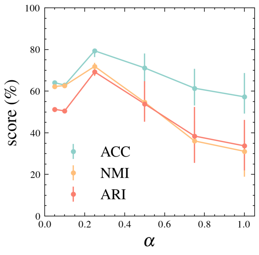
(b)

AG News

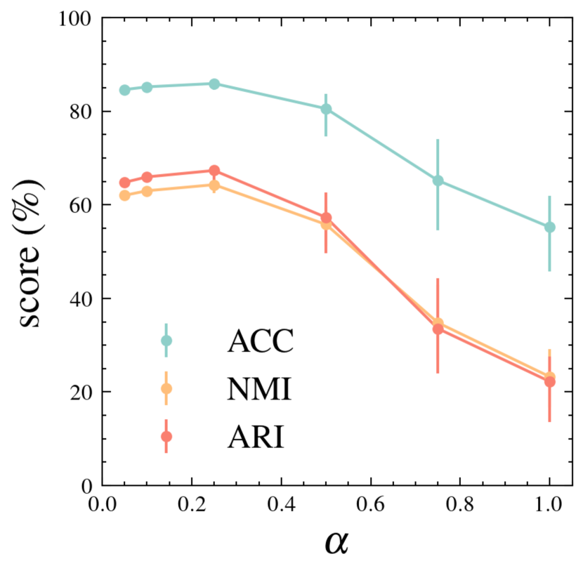
(c)

Yahoo! Answers

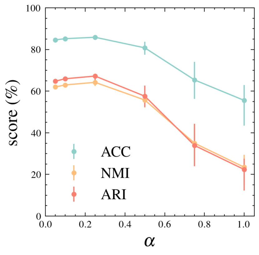
(d)

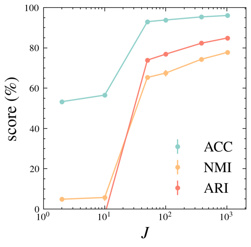
(e)

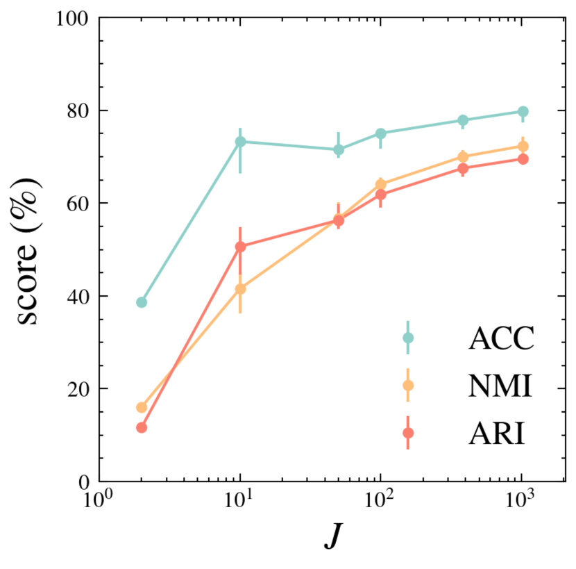
(f)

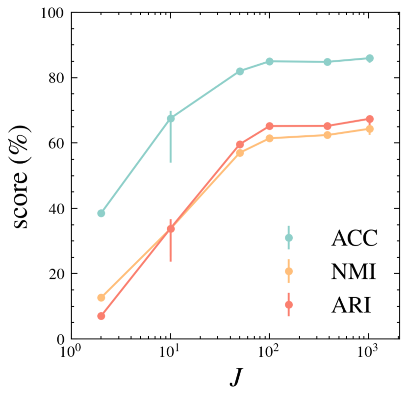
(g)

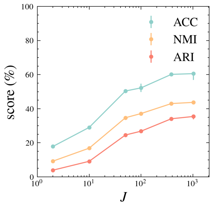
(h)

Figure 1: Performance of GC on the four datasets (columns) with varying (a-d) $\alpha$ values or (e-h) $J$ values. Different colors represent different clustering evaluation metrics, with error bars indicating the 95% confidence interval, based on 100 repeated experiments. Error bars for some $\alpha$ and $J$ values are too small to be visible.

Ablated versions.

The bottom of Table 6.1 shows the results for three ablated versions of GC. These versions used $\alpha=1$ instead of the recommended $\alpha=0.25$, estimated the proposal distribution $p(Y)$ with a naïve estimator instead of Eq. (7), and omitted the probability clipping step in Eq. (11).

The largest performance loss occurred with $\alpha=1.00$ instead of $\alpha=0.25$, an interesting outcome that we discuss in Section 8. Results for other $\alpha$ values are given in Figures 1(a-d) for the four datasets. $\alpha=0.25$ consistently yielded the best performance across all datasets. The plots represent mean values over 100 repeated experiments, with error bars indicating the 95% confidence interval.

Figures 1(e-h) show the performance as a function of the sample size $J$ for the four datasets. The plots represent mean values from 100 repeated experiments, with error bars indicating 95% confidence intervals. Increasing $J$ requires generating and evaluating more texts, but it yields higher clustering scores and more stable outcomes. On smaller datasets (R2, R5 and AG News), performance curves converged for $J\geq 50$. For the largest dataset, Yahoo! Answers, convergence was evident at $J\geq 384$, which is smaller than the typically dimensionality of BERT embeddings (768).

The probability clipping step also brought consistent improvement across all datasets. As for using a naïve estimator for $p(Y)$, the performance decrease was less severe, but still noticeable on the R2 and the AG News datasets.

Clustering with misspecified $K$

We also evaluated GC with misspecified numbers of clusters, $K$. Results are summarized in Appendix B.2. With $K$ misspecified, GC and SBERT-based methods suffered performance degradation, but GC still steadily outperformed SBERT-based methods across all tested $K$ values from 2 to 20. This suggests the robustness of GC to the choice of $K$.

7 Application to Generative Retrieval

Among vast application possibilities, GC can be naturally applied to generative document retrieval (GDR), (Tay et al. 2022). In GDR, the $\mathrm{Y}$ are queries for the retrieval, and documents $\mathrm{X}$ are indexed by using prefix coding, which necessitates hierarchical clustering.

7.1 Hierarchical Clustering with Localized $\phi$

Algorithm 2 Hierarchical clustering.

Input: Documents $\tilde{\mathrm{X}}\subset\mathrm{X}$ in a sub-cluster; the generated texts $\mathrm{Y}=\{y_{1},\cdots,y_{J}\}$ and the probability matrix $\mathbf{P}$ produced in Algorithm 1 (for the whole $\mathrm{X}$).

Parameters: Number of clusters, $K$; number of text samples, $J$; proposal distribution, $\phi(Y)$; regularization factor, $\alpha$. Output: Cluster assignment function $f:\mathrm{X}\to\{1,2,\cdots,K\}$.

1:

For $y_{j}\in\mathrm{Y}$, estimate $\tilde{\phi}(y_{j})$ using only the documents in $\tilde{\mathrm{X}}$.

Eq.(7)

2:

Calculate the resampling weights $\mathbf{r}_{j}$.

Eq.(12)

3:

Resample $J$ texts from $\mathrm{Y}$ according to the weights $\mathbf{r}_{j}$, forming $\tilde{\mathrm{Y}}$ and correspondingly, $\tilde{\mathbf{P}}$, which is a reselection of $\mathbf{P}$’s columns with replacement.

4:

Compute the importance weight matrix
$\tilde{\mathbf{W}}_{ij}=\left(\tilde{\mathbf{P}}_{ij}/\tilde{\phi}(y_{j})\right)^{\alpha}$.

5:$f\leftarrow\textsc{Clustering}(\tilde{\mathbf{P}},\tilde{\mathbf{W}})$ from Algorithm 1.

The clustering in Algorithm 1 can be extended to a hierarchical version, given as Algorithm 7.1. When clustering documents within a sub-cluster $\tilde{\mathrm{X}}\subset\mathrm{X}$, the proposal distribution $\phi$ is localized to this sub-cluster for improved KL divergence estimation and denoted as $\tilde{\phi}$. This localized distribution is estimated using Eq. (7) with sub-cluster documents (see Appendix A.3 for the details).

We apply bootstrapping to generate samples from $\tilde{\phi}$ without recalculating $\mathbf{P}$. Resampling is performed from $\mathrm{Y}=[y_{1},\cdots,y_{J}]$ with weights $\mathbf{r}$:

$$\mathbf{r}_{j}=\left(\dfrac{\tilde{\phi}(y_{j})}{\phi(y_{j})}\right)^{\alpha}$$ (12)

Repeating this resampling $J$ times generates a new text set $\tilde{\mathrm{Y}}$, with its corresponding localized probability matrix $\tilde{\mathbf{P}}$ and importance weights $\tilde{\mathbf{W}}$ derived from $\mathbf{P}$ and $\tilde{\phi}$. Then, $\tilde{\mathrm{X}}$ is clustered by the iterative procedure in Algorithm 1 with these localized matrices.

7.2 Document Indexing Through Hierarchical Clustering

In GDR, documents are indexed using a prefix code generated by hierarchical clustering. Each document is assigned a unique numerical string based on its cluster index at each level of the hierarchy.

Previous methods used BERT-based vectors and $k$-means for this prefix code construction, as in DSI (Tay et al. 2022) and NCI (Wang et al. 2022). Recently, Du, Xiu, and Tanaka-Ishii (2024) proposed query-based document clustering, but using BERT and $k$-means clustering, which should be improved upon by our method.

After constructing the prefix code, a neural retrieval model is trained to map queries to the numerical strings of their corresponding documents. The clustering method’s effectiveness was evaluated via the retrieval accuracy. We used the same setting as in Wang et al. (2022) for the retrieval model and the training details. In other words, the only change was the construction of document indexes with our GC instead of $k$-means. Our indexing method is abbreviated as GCI. We set $K=30$ and $J=4096$.

We compared our method with NCI and BMI, which use hierarchical $k$-means clustering for document indexing. We used a small retrieval model with about 30M parameters to highlight the clustering method’s advantage. Two datasets, NQ320K (Kwiatkowski et al. 2019) and MS Marco Lite (Du, Xiu, and Tanaka-Ishii 2024), were used for evaluation, with the numbers of documents listed in the top row of Table 3. We fine-tuned the doc2query models on the two datasets.

7.3 Results

	MS Marco Lite		NQ320K
	(138,457 docs.)		(109,739 docs.)
	Rec@1	MRR100	Rec@1	MRR100
NCI	17.91	28.82	44.70	56.24
BMI	23.78	35.51	55.17	65.52
[0.5pt/1pt] ours
GCI ($\alpha=0.25$, $J=4096$)	32.41	44.36	56.40	66.20
Ablated versions
- $\alpha=0.1$	31.66	44.12	55.53	65.74
- $\alpha=0.5$	29.80	40.93	53.97	64.13
- $\alpha=1$	24.43	36.13	47.87	58.84
- $J=1024$	32.16	44.02	56.19	65.94
- $J=300$	29.08	40.93	53.62	64.07
- No localized $\phi$	30.37	42.26	55.20	65.41

Table 3: Retrieval accuracies on document indexes acquired with different clustering methods, using a T5 retrieval model with $\sim$ 30M parameters. The best scores are in bold.

The upper half of Table 3 compares the different clustering-based indexing methods. On MS Marco Lite, BMI outperformed NCI, and our GCI significantly outperformed both. Compared with BMI, our method achieved an 8.63 (36%) increase in Recall@1 and an 8.85 (25%) increase in MRR@100.

Ablation tests (lower half of Table 3) showed consistency with the clustering evaluations reported in Table 6.1. The best retrieval performance was achieved by $\alpha=0.25$, suggesting that it is a robust choice for both clustering and generative retrieval. Moreover, while reducing the sample size $J$ to smaller values (1024 and 300) decreased the retrieval accuracy, the performance loss was insignificant for $J=1024$ compared to $J=4096$. Furthermore, skipping the localization of $\phi$ to sub-clusters (last row of Table 6.1) also reduced the retrieval accuracy.

8 Discussions

Bias-Variance Tradeoff

Previous research on importance sampling primarily focused on reducing variance while maintaining an unbiased estimator (i.e., $\mathbb{E}[\hat{d}]=d$), typically using $\alpha=1$ in Eq. (5) (Owen and Zhou 2000). However, clustering requires no such constraint of unbiasedness, as the clustering results are invariant to scaling of $\hat{d}$ and robust to bias.

On the other hand, lowering $\alpha$ has a significant impact on reducing the variance (or uncertainty) of the estimator $\hat{d}$, which is crucial for $\hat{d}$ to reliably recover the true clustering structure of $d$. For language models, the probabilities $p(Y|x)$ are typically right-skewed severely, akin to the log-normal distribution, and reducing $\alpha$ can exponentially reduce the variance of the estimator. This can be analyzed through the notion of effective sample size (Hesterberg 1995). This explains why reducing $\alpha$ from 1 to 0.25 significantly improved the NMI on the R2 dataset from 25.8% to 77.8% (Table 6.1).

However, too much reduction in $\alpha$ can lead to distortion of information, and as the benefits of variance reduction diminish, the bias dominates the error. As shown in Figures 1(a-b), reducing $\alpha$ below 0.25 decreased the clustering performance. This reveals a tradeoff between bias and variance in the importance sampling estimation of the KL divergence.

Choice of Language Model

We have focused on using the doc2query family of models (Nogueira, Lin, and Epistemic 2019) in our experiments, which are pretrained to generate queries from documents. This choice is motivated by observing many real-world datasets to be organized around queries or topics, in addition to the content of the documents themselves. Nevertheless, the doc2query models were not specifically designed for clustering, and how to fine-tune language models for clustering is an interesting future research direction.

Computational Complexity

The primary computational cost of our method is the calculation of the probability matrix $\mathbf{P}$, which requires evaluating $p(y|x)$ for each pair of documents and queries. This cost can be reduced by caching LLM states of $x$ and using low-precision inference. We used the BF16 precision in our experiments and observed no significant performance loss. On the R2 dataset, for example, calculation of $\mathbf{P}$ finishes within 10 minutes on a single GPU.

9 Conclusion

This paper explored using generative large language models (LLMs) to enhance document clustering. By translating documents into a broader representation space, we captured richer information, leading to a more effective clustering approach using the KL divergence.

Our results showed significant improvements across multiple datasets, indicating that LLM-enhanced representations improve clustering structure recovery. We also proposed an information-theoretic clustering method based on importance sampling, which proved effective and robust across all tested datasets. Additionally, our method improved the retrieval accuracy in generative document retrieval (GDR), demonstrating its potential for wide-ranging applications.

Acknowledgments

This work was supported by JST CREST Grant Number JPMJCR2114. We thank the anonymous reviewers for their valuable comments and suggestions.

Technical Appendices fo

Information-Theoretic Generative Clustering of Documents

Appendix A Mathematical Details

A.1 Convergence of the Clustering Algorithm

Proposition 1.

Algorithm 1 converges to a local minimum of the total distortion:

$$D\equiv\sum_{x\in\mathrm{X}}\hat{d}(x,f(x)),$$ (13)

where $\hat{d}$ is defined in Eq. (5).

Proof.

The generative clustering algorithm 1 employs a two-step iterative process to alternately update the cluster assignment function $f:\mathrm{X}\mapsto\{1,2,\cdots,K\}$ and the cluster centroids $\mathbf{c}_{k}$. Because the total distortion $D$ decreases after each update of the cluster assignment function $f$ and the cluster centroids $\mathbf{c}_{k}$, the algorithm converges to a local minimum of $D$. ∎

However, convergence to a global optimum is not guaranteed, as this is a more general and much challenging problem, which is not addressed in this paper. In practice, we find that using random initialization with different seeds and performing model selection based on total distortion, similar to the approach used in $k$-means, improves clustering performance.

A.2 Optimal Cluster Centroid

Proposition 2.

(Distortion-minimal cluster centroid) For a cluster $k$, the within-cluster total distortion

$$D_{k}(\mathbf{c}_{k})\equiv\sum_{x\in f^{-1}(k)}\hat{d}(x,f(x))=\sum_{x_{i}\in f^{-1}(k)}\frac{1}{J}\sum_{j=1}^{J}\mathbf{W}_{ij}\log\frac{\mathbf{P}_{ij}}{\mathbf{c}_{k}(j)}$$ (14)

with respect to the cluster centroid $\mathbf{c}_{k}$, subject to $\sum_{j=1}^{J}\mathbf{c}_{k}(j)=1$, is minimized at:

$$\mathbf{c}_{k}^{*}(j)=\frac{1}{Z}\sum_{x_{i}\in f^{-1}(k)}\mathbf{W}_{ij},~{}~{}~{}~{}j=1,2,\cdots,J,$$ (15)

where $Z=\sum_{j=1}^{J}\mathbf{c}_{k}^{*}(j)$ is the normalization term.

This proposition is similar to that for Bregman hard clustering problem (Banerjee et al. 2005). We provide a proof via the Lagrange multiplier method in the following.

Proof.

Rearranging Eq. (14), we obtain:

$$D_{k}(\mathbf{c}_{k}) =\frac{1}{J}\sum_{j=1}^{J}\sum_{x_{i}\in f^{-1}(k)}\mathbf{W}_{ij}\log\frac{\mathbf{P}_{ij}}{\mathbf{c}_{k}(j)}$$ (16)

$$=-\frac{1}{J}\sum_{j=1}^{J}\mathbf{w}_{k}(j)\log\mathbf{c}_{k}(j)+\text{constant},$$ (17)

where $\mathbf{w}_{k}(j)=\sum_{x_{i}\in f^{-1}(k)}\mathbf{W}_{ij}$.

Using the Lagrange multiplier method to incorporate the constraint, the Lagrangian is given by:

$$L(D_{k},\lambda)=D_{k}(\mathbf{c}_{k})+\lambda\left(\sum_{j=1}^{J}\mathbf{c}_{k}(j)-1\right).$$ (19)

Taking the derivative of $L$ with respect to $\mathbf{c}_{k}(j)$ for every $j$, we get:

$$\frac{\partial L}{\partial\mathbf{c}_{k}^{*}(j)}=-\frac{\mathbf{w}_{k}(j)}{J\mathbf{c}_{k}^{*}(j)}+\lambda=0.$$ (20)

This implies:

$$\frac{\mathbf{w}_{k}(1)}{\mathbf{c}_{k}^{*}(1)}=\cdots=\frac{\mathbf{w}_{k}(J)}{\mathbf{c}_{k}^{*}(J)}=J\lambda.$$ (21)

Using $\sum_{j=1}^{J}\mathbf{c}_{k}^{*}(j)=1$ again, we derive the optimal solution:

$$\mathbf{c}_{k}^{*}(j)=\frac{1}{Z}\mathbf{w}_{k}(j)=\frac{1}{Z}\sum_{x_{i}\in f^{-1}(k)}\mathbf{W}_{ij},$$ (22)

where $Z=\sum_{j=1}^{J}\mathbf{c}_{k}^{*}(j)$ is the normalization term. This completes the proof of Proposition 5.4. ∎

A.3 The Second-Moment-Minimizing Proposal $\phi(Y)$

As discussed in Section 5.2, we use importance sampling to estimate $\mathbb{E}_{Y\sim p(Y|x)}\log\frac{p(Y|x)}{p(Y|k)}$ (the KL divergence between document $x$ and cluster centroid $k$) by employing an alternative distribution $\phi$, known as the proposal distribution:

$$\mathbb{E}_{Y\sim p(Y|x)}\log\frac{p(Y|x)}{p(Y|k)}=\mathbb{E}_{Y\sim\phi}\frac{p(Y|x)}{\phi(Y)}\log\frac{p(Y|x)}{p(Y|k)}.$$ (23)

In importance sampling, large variation in the importance weights $\frac{p(Y|x)}{\phi(Y)}$ can lead to unreliable estimates of the KL divergence. To minimize this variance, choosing $\phi(Y)=p(Y|x)$ would be ideal, as it reduces the variance to zero. However, since $\phi$ is shared across all documents in $\mathrm{X}$, it should be selected to minimize the overall variance across all $p(Y|x)$ distributions, rather than for any specific document.

This intuition can be realized by minimizing the second moment of the importance weights:

$$\mathbb{E}_{\phi(Y)}\left[\left(\frac{p(Y|X)}{\phi(Y)}\right)^{2\alpha}\right]=\mathrm{Var}_{\phi(Y)}\left(\frac{p(Y|X)}{\phi(Y)}\right)^{\alpha}+\left\{\mathbb{E}_{\phi(Y)}\left[\left(\frac{p(Y|X)}{\phi(Y)}\right)^{\alpha}\right]\right\}^{2},$$ (24)

This idea is formalized in the following proposition.

Proposition 3.

(Second-moment-minimizing proposal $\phi^{*}$) The second moment of the importance weights,

$$M(\phi)\equiv\mathbb{E}_{X}\mathbb{E}_{\phi(Y)}\left[\left(\frac{p(Y|X)}{\phi(Y)}\right)^{2\alpha}\right]$$ (25)

subject to the normalization condition $\sum_{y\in\mathcal{Y}}\phi(y)=1$, is minimized by:

$$\phi^{*}(y)=\frac{1}{Z}\left(\mathbb{E}_{X}\left[p(y|X)^{2\alpha}\right]\right)^{1/2\alpha}~{}~{}~{}~{}~{}~{}\forall y\in\mathcal{Y},$$ (26)

where $Z=\sum_{y\in\mathcal{Y}}\phi^{*}(y_{j})$ is the normalization term.

Proof.

The constraint is incorporated using the Lagrange multipler method, with the following Lagrangian:

$$L(\phi,\lambda)=M(\phi)+\lambda\left(\sum_{y\in\mathcal{Y}}\phi(y)-1\right).$$ (27)

Take the partial derivative of $L$ with respect to $\phi(y)$ for any $y$. We have:

$$\frac{\partial L}{\partial\phi(y)} =\frac{\partial}{\partial\phi(y)}\left[\mathbb{E}_{X}\left(\sum_{y\in\mathcal{Y}}^{J}p(y|X)^{2\alpha}\phi(y)^{1-2\alpha}\right)+\lambda\left(\sum_{y\in\mathcal{Y}}\phi(y)-1\right)\right]$$ (28)

$$=(1-2\alpha)\mathbb{E}_{X}[p(y|X)^{2\alpha}]\phi(y)^{-2\alpha}+\lambda.$$ (29)

Equating these derivatives to zero:

$$\frac{\phi^{*}(y)}{\mathbb{E}_{X}[p(y|X)^{2\alpha}]^{1/2\alpha}}=\left(\frac{2\alpha-1}{\lambda}\right)^{1/2\alpha}\quad\forall y\in\mathcal{Y}.$$ (30)

which are identical for all $y\in\mathcal{Y}$. Thus,

$$\phi^{*}(y)\propto\left(\mathbb{E}_{X}\left[p(y|X)^{2\alpha}\right]\right)^{1/2\alpha}\quad\forall y\in\mathcal{Y}.$$ (31)

Scaling $\phi^{*}$ to satisfy the constraint $\sum_{y\in\mathcal{Y}}\phi(y)=1$ yields the expression in Eq. (26), completing the proof.

∎

Nevertheless, since $\mathcal{Y}$ is infinite, $Z$ is not computable. Fortunately, $Z$ can be factored out from $\hat{d}(x,k)$, meaning that setting $Z$ to any positive value will yield the same cluster assignment and not affect the clustering procedure. Thus, we set $Z=1$ in the paper, leading to Eq. (7).

Localized proposal $\tilde{\phi}$.

In a hierarchical clustering on $\mathrm{X}$, the clustering algorithm 1 is recursively applied to subclusters, denoted as $\tilde{\mathrm{X}}$, as discussed in Section 7.1. The second-moment-minimizing proposal is then computed using documents in $\tilde{\mathrm{X}}$ instead of $\mathrm{X}$:

$$\tilde{\phi}^{*}(y)\leftarrow\left(\frac{1}{|\tilde{\mathrm{X}}|}\sum_{x\in\tilde{\mathrm{X}}}p(y|x)^{2\alpha}\right)^{1/2\alpha}.$$ (32)

Appendix B Additional Experiments

B.1 Initialization by $k$-means++

A more sophisticated initialization method, $k$-means++, can be adapted to our clustering algorithm. In the $k$-means algorithm and our Algorithm 1, the cluster centroids are initialized by randomly selecting $K$ documents. The $k$-means++ algorithm (Arthur and Vassilvitskii 2006) improves this initialization by selecting documents that are far apart from each other, thus reducing the risk of converging to a suboptimal solution.

The $k$-means++ method used the following initialization procedure:

1. Randomly select the first centroid $\mathbf{c}_{1}$ from the document set $\mathrm{X}$ according to the uniform distribution.

2. Selecting the next cluster centroid $c_{i}$ as $x^{\prime}\in\mathrm{X}$ with probability $\dfrac{d(x^{\prime})^{2}}{\sum_{x\in\mathrm{X}}d(x)^{2}}$, where $d(x)$ denote the Euclidean distance between $x$ and the nearest centroid already chosen.

3. Repeat Step b until $K$ centroids are selected.

In our approach, the centroids $c_{i}$ are represented by the importance weights of the selected documents, each normalized to sum to 1, as in Eq. (10). Moreover, because the estimated KL divergence used in our algorithm is not necessarily positive, we modify the distance $d(x)$ used for $k$-means++ initialization as follows: at iteration $i$,

$$d(x) \leftarrow\min_{k=1,\cdots,i-1}\hat{d}(x,k)\quad\forall x\in\mathrm{X}$$ (33)

$$d(x) \leftarrow d(x)-\min_{x\in\mathrm{X}}d(x),$$ (34)

where $\hat{d}(x,k)$ is the estimated KL divergence between $x$ and cluster $k$ using the RIS estimator in Eq. (5). This modification offsets the estimated KL divergence, such that $d(x)\geq 0$, and the probability of selecting a document $x$ as the next centroid to be exactly zero if it has the smallest estimated KL divergence to the nearest centroid.

Initialization	R2			R5			AG News			Yahoo! Answers
The selected run with minimal total distortion, averaged over 100 repeated experiments
Random	96.1	77.8	84.9	79.1	71.5	69.1	85.9	64.2	67.2	60.7	43.8	35.5
$k$-means++	96.1	77.8	84.9	79.8	72.0	69.6	85.9	64.3	67.3	60.5	43.7	35.5
Single run, averaged over 100 repeated experiments
Random	89.0	65.9	69.4	72.7	67.4	63.5	77.0	59.9	58.5	55.8	42.4	33.4
$k$-means++	89.6	66.1	69.8	72.4	67.5	63.3	77.4	60.2	59.3	55.5	42.2	33.2

Table 4: Results of the $k$-means++ initialization compared with random initialization on four datasets.

We tested the $k$-means++ initialization on the datasets in Table 1, comparing it with the default random initialization. The results are shown in Table 4. The upper half of the table was acquired with the same setting as in the main text (Table 6.1), i.e., with a selecting procedure on ten different seeds. The lower half of the table shows the results without the selecting procedure. All results are averaged over 100 repeated experiments.

The $k$-means++ initialization did not significantly improve the clustering performance compared with random initialization, either with or without the selecting procedure. This could be because the datasets used in our experiments have relatively smaller numbers of clusters, making the impact of initialization less significant.

B.2 Clustering with Misspecified Number of Clusters

$K$	2	4	5*	6	10	20
SBERT (All-minilm-l12-v2)	31.9	53.7	58.6	50.8	37.9	21.9
GC (ours)	53.9	64.5	69.1	59.8	38.6	22.0

Table 5: Clustering performance on the R5 dataset with misspecified number of clusters, measured by Adjusted Rand Index (ARI). The ground-truth number of clusters is 5, as marked with an asterisk.

Table 5 shows the clustering performance on the R5 dataset when the number of clusters $K$ is misspecified. The ground-truth number of clusters is 5. Our GC (last row) is compared with the best-performing SBERT-based method on this dataset (first row).

When the number of clusters is misspecified, the clustering performance of the two methods degraded. However, our method still outperformed the SBERT-based method in all cases. This suggests that our method is robust to misspecified $K$ values and is effective in real-world applications where the number of clusters is unknown.

References

- Aouali et al. (2024) Aouali, I.; Brunel, V.-E.; Rohde, D.; and Korba, A. 2024. Unified PAC-Bayesian Study of Pessimism for Offline Policy Learning with Regularized Importance Sampling. arXiv preprint arXiv:2406.03434.
- Arthur and Vassilvitskii (2006) Arthur, D.; and Vassilvitskii, S. 2006. k-means++: The advantages of careful seeding. Technical report, Stanford.
- Banerjee et al. (2005) Banerjee, A.; Merugu, S.; Dhillon, I. S.; Ghosh, J.; and Lafferty, J. 2005. Clustering with Bregman divergences. Journal of machine learning research, 6(10).
- Blei, Ng, and Jordan (2003) Blei, D. M.; Ng, A. Y.; and Jordan, M. I. 2003. Latent dirichlet allocation. Journal of machine Learning research, 3(Jan): 993–1022.
- Devlin et al. (2019) Devlin, J.; Chang, M.-W.; Lee, K.; and Toutanova, K. 2019. BERT: Pre-training of Deep Bidirectional Transformers for Language Understanding. In Burstein, J.; Doran, C.; and Solorio, T., eds., Proceedings of the 2019 Conference of the North American Chapter of the Association for Computational Linguistics: Human Language Technologies, Volume 1 (Long and Short Papers), 4171–4186. Minneapolis, Minnesota: Association for Computational Linguistics.
- Dhillon, Mallela, and Modha (2003) Dhillon, I. S.; Mallela, S.; and Modha, D. S. 2003. Information-theoretic co-clustering. In Proceedings of the ninth ACM SIGKDD international conference on Knowledge discovery and data mining, 89–98.
- Du, Xiu, and Tanaka-Ishii (2024) Du, X.; Xiu, L.; and Tanaka-Ishii, K. 2024. Bottleneck-Minimal Indexing for Generative Document Retrieval. In Forty-first International Conference on Machine Learning.
- Guan et al. (2022) Guan, R.; Zhang, H.; Liang, Y.; Giunchiglia, F.; Huang, L.; and Feng, X. 2022. Deep feature-based text clustering and its explanation. IEEE Transactions on Knowledge and Data Engineering, 34(8): 3669–3680.
- Gulli (2005) Gulli, A. 2005. AG news homepage.
- Guo et al. (2017) Guo, X.; Gao, L.; Liu, X.; and Yin, J. 2017. Improved deep embedded clustering with local structure preservation. In Ijcai, volume 17, 1753–1759.
- Hesterberg (1995) Hesterberg, T. 1995. Weighted average importance sampling and defensive mixture distributions. Technometrics, 37(2): 185–194.
- Hubert and Arabie (1985) Hubert, L.; and Arabie, P. 1985. Comparing partitions. Journal of classification, 2: 193–218.
- Kloek and Van Dijk (1978) Kloek, T.; and Van Dijk, H. K. 1978. Bayesian estimates of equation system parameters: an application of integration by Monte Carlo. Econometrica: Journal of the Econometric Society, 1–19.
- Kojima et al. (2022) Kojima, T.; Gu, S. S.; Reid, M.; Matsuo, Y.; and Iwasawa, Y. 2022. Large language models are zero-shot reasoners. Advances in neural information processing systems, 35: 22199–22213.
- Korba and Portier (2022) Korba, A.; and Portier, F. 2022. Adaptive importance sampling meets mirror descent: a bias-variance tradeoff. In International Conference on Artificial Intelligence and Statistics, 11503–11527. PMLR.
- Kwiatkowski et al. (2019) Kwiatkowski, T.; Palomaki, J.; Redfield, O.; Collins, M.; Parikh, A.; Alberti, C.; Epstein, D.; Polosukhin, I.; Devlin, J.; Lee, K.; et al. 2019. Natural questions: a benchmark for question answering research. Transactions of the Association for Computational Linguistics, 7: 453–466.
- Mikolov et al. (2013) Mikolov, T.; Sutskever, I.; Chen, K.; Corrado, G. S.; and Dean, J. 2013. Distributed representations of words and phrases and their compositionality. Advances in neural information processing systems, 26.
- Nguyen, Wainwright, and Jordan (2010) Nguyen, X.; Wainwright, M. J.; and Jordan, M. I. 2010. Estimating divergence functionals and the likelihood ratio by convex risk minimization. IEEE Transactions on Information Theory, 56(11): 5847–5861.
- Nogueira, Lin, and Epistemic (2019) Nogueira, R.; Lin, J.; and Epistemic, A. 2019. From doc2query to docTTTTTquery. Online preprint, 6: 2.
- OpenAI (2023) OpenAI. 2023. Gpt-4 technical report. arXiv preprint arXiv:2303.08774.
- Owen and Zhou (2000) Owen, A.; and Zhou, Y. 2000. Safe and effective importance sampling. Journal of the American Statistical Association, 95(449): 135–143.
- Pérez-Cruz (2008) Pérez-Cruz, F. 2008. Kullback-Leibler divergence estimation of continuous distributions. In 2008 IEEE international symposium on information theory, 1666–1670. IEEE.
- Peters et al. (2018) Peters, M. E.; Neumann, M.; Iyyer, M.; Gardner, M.; Clark, C.; Lee, K.; and Zettlemoyer, L. 2018. Deep Contextualized Word Representations. In Walker, M.; Ji, H.; and Stent, A., eds., Proceedings of the 2018 Conference of the North American Chapter of the Association for Computational Linguistics: Human Language Technologies, Volume 1 (Long Papers), 2227–2237. New Orleans, Louisiana: Association for Computational Linguistics.
- Raffel et al. (2020) Raffel, C.; Shazeer, N.; Roberts, A.; Lee, K.; Narang, S.; Matena, M.; Zhou, Y.; Li, W.; and Liu, P. J. 2020. Exploring the limits of transfer learning with a unified text-to-text transformer. The Journal of Machine Learning Research, 21(1): 5485–5551.
- Reimers and Gurevych (2019) Reimers, N.; and Gurevych, I. 2019. Sentence-BERT: Sentence Embeddings using Siamese BERT-Networks. In Proceedings of the 2019 Conference on Empirical Methods in Natural Language Processing. Association for Computational Linguistics.
- Slonim and Tishby (2000) Slonim, N.; and Tishby, N. 2000. Document clustering using word clusters via the information bottleneck method. In Proceedings of the 23rd annual international ACM SIGIR conference on Research and development in information retrieval, 208–215.
- Subakti, Murfi, and Hariadi (2022) Subakti, A.; Murfi, H.; and Hariadi, N. 2022. The performance of BERT as data representation of text clustering. Journal of big Data, 9(1): 15.
- Tay et al. (2022) Tay, Y.; Tran, V.; Dehghani, M.; Ni, J.; Bahri, D.; Mehta, H.; Qin, Z.; Hui, K.; Zhao, Z.; Gupta, J.; Schuster, T.; Cohen, W. W.; and Metzler, D. 2022. Transformer Memory as a Differentiable Search Index. In Koyejo, S.; Mohamed, S.; Agarwal, A.; Belgrave, D.; Cho, K.; and Oh, A., eds., Advances in Neural Information Processing Systems, volume 35, 21831–21843. Curran Associates, Inc.
- Vinh, Epps, and Bailey (2010) Vinh, N. X.; Epps, J.; and Bailey, J. 2010. Information Theoretic Measures for Clusterings Comparison: Variants, Properties, Normalization and Correction for Chance. Journal of Machine Learning Research, 11(95): 2837–2854.
- Viswanathan et al. (2023) Viswanathan, V.; Gashteovski, K.; Lawrence, C.; Wu, T.; and Neubig, G. 2023. Large language models enable few-shot clustering. arXiv preprint arXiv:2307.00524.
- Wang, Kulkarni, and Verdú (2009) Wang, Q.; Kulkarni, S. R.; and Verdú, S. 2009. Divergence estimation for multidimensional densities via -Nearest-Neighbor distances. IEEE Transactions on Information Theory, 55(5): 2392–2405.
- Wang et al. (2022) Wang, Y.; Hou, Y.; Wang, H.; Miao, Z.; Wu, S.; Sun, H.; Chen, Q.; Xia, Y.; Chi, C.; Zhao, G.; Liu, Z.; Xie, X.; Sun, H.; Deng, W.; Zhang, Q.; and Yang, M. 2022. A Neural Corpus Indexer for Document Retrieval. In Oh, A. H.; Agarwal, A.; Belgrave, D.; and Cho, K., eds., Advances in Neural Information Processing Systems.
- Wu et al. (2020) Wu, Y.; Zhou, P.; Wilson, A. G.; Xing, E.; and Hu, Z. 2020. Improving gan training with probability ratio clipping and sample reweighting. Advances in Neural Information Processing Systems, 33: 5729–5740.
- Xie, Girshick, and Farhadi (2016) Xie, J.; Girshick, R.; and Farhadi, A. 2016. Unsupervised deep embedding for clustering analysis. In International conference on machine learning, 478–487. PMLR.
- Xu et al. (2017) Xu, J.; Xu, B.; Wang, P.; Zheng, S.; Tian, G.; and Zhao, J. 2017. Self-taught convolutional neural networks for short text clustering. Neural Networks, 88: 22–31.
- Yang et al. (2022) Yang, X.; Yan, J.; Cheng, Y.; and Zhang, Y. 2022. Learning deep generative clustering via mutual information maximization. IEEE Transactions on Neural Networks and Learning Systems, 34(9): 6263–6275.
- Yin and Wang (2014) Yin, J.; and Wang, J. 2014. A dirichlet multinomial mixture model-based approach for short text clustering. In Proceedings of the 20th ACM SIGKDD international conference on Knowledge discovery and data mining, 233–242.
- Zhang, Zhao, and LeCun (2015) Zhang, X.; Zhao, J.; and LeCun, Y. 2015. Character-level convolutional networks for text classification. Advances in neural information processing systems, 28.
- Zhang, Wang, and Shang (2023) Zhang, Y.; Wang, Z.; and Shang, J. 2023. Clusterllm: Large language models as a guide for text clustering. arXiv preprint arXiv:2305.14871.
- Zhong and Ghosh (2005) Zhong, S.; and Ghosh, J. 2005. Generative model-based document clustering: a comparative study. Knowledge and Information Systems, 8: 374–384.
- Zhou et al. (2022) Zhou, S.; Xu, H.; Zheng, Z.; Chen, J.; Bu, J.; Wu, J.; Wang, X.; Zhu, W.; Ester, M.; et al. 2022. A comprehensive survey on deep clustering: Taxonomy, challenges, and future directions. arXiv preprint arXiv:2206.07579.