Squint-Aware ISAC Precoding Towards Enhanced Dual-Functional Gain in Sub-Terahertz Systems

Abstract

The potential benefits of integrated sensing and communication (ISAC) are anticipated to play a significant role in future sub-terahertz (sub-THz) systems. However, the beam squint effect is pronounced in sub-THz systems, expanding coverage areas while severely degrading communication performance. Existing hybrid precoding designs struggle to balance both functionalities in the presence of beam squint, limiting the performance gain achievable through ISAC. To address this challenge, we propose two squint-aware hybrid precoding schemes for sub-THz systems that proactively regulate the correlation between communication and sensing channels, leveraging the inherent degrees of freedom in the hardware to enhance integrated gain. We introduce a squint-aware optimization-based hybrid precoding algorithm (SA-Opt) and develop an unsupervised learning-assisted complex-valued squint-aware network (CSP-Net) to reduce complexity, tailoring its architecture to the specific data and task characteristics. The effectiveness of the proposed schemes is demonstrated through simulations.

I Introduction

Integrated sensing and communication (ISAC) serves as a technological cornerstone for supporting emerging applications such as vehicular networks and the low-altitude economy [1, 2, 3]. To achieve higher data rates, larger antenna arrays operating at higher frequencies have been adopted [4], leading to the development of sub-terahertz (sub-THz) communication systems. Meanwhile, these sub-THz systems enhance distance and angle resolution, making the integration of communication and sensing a promising avenue.

However, the beam squint effect becomes pronounced in the sub-THz systems [5], significantly reducing the antenna array gain and deteriorating communication performance. To mitigate this issue, the true time delay (TTD) has been introduced in hybrid precoding, providing frequency-dependent phase shifts that ensure beam alignment across subcarriers [6]. Conversely, for sensing tasks, beam squint can lead to wider coverage and enhanced frequency-aware angle estimation capabilities. For instance, studies in [7, 8] worked on controlling the pattern of beam squint through TTDs, facilitating user localization or target angle estimation. Nevertheless, current sub-THz systems lack a joint design for both functionalities, failing to achieve optimal trade-offs. This motivates us to implement ISAC under the beam squint effect.

It is worth noting that the correlation between communication and sensing channels affects the performance gain when both functionalities co-exist [9, 10]. Previous studies such as [11] evaluated this channel correlation from the perspective of power sharing. However, they do not provide direct guidance for precoding design. Moreover, transmitters fail to actively manipulate the degree of correlation between channels. [12, 13] improved the channel correlation through reconfigurable intelligent surfaces, thereby enhancing ISAC performance. However, these methods are primarily limited to narrowband systems and may exacerbate beam squint effects in sub-THz systems. In fact, hybrid precoding systems possess their own design degrees of freedom that can be leveraged to tune the channel correlation, which has not been thoroughly explored. Notably, the TTD serves to adjust spatial-domain fading across subcarriers, holding the potential in inherently tuning the channel correlation.

Inspired by this, in this paper, we propose squint-aware ISAC hybrid precoding schemes for sub-THz systems in the presence of beam squint effect, without altering existing hardware architectures. Specifically, we first propose a C-S channel correlation metric as the foundation. Then we design the TTDs to proactively manipulate the equivalent channels for correlation maximization, followed by an alternating optimization of the phase shifters (PSs) and power allocation to achieve the ISAC Pareto boundary. While this optimization-based algorithm addresses the problem with near-optimal performance, the iterative and exhaustive search processes involve high complexity, particularly under large arrays. Hence we also propose an unsupervised learning-aided scheme for ISAC hybrid precoding design with reduced complexity. Unlike [14, 15], we tailor the network architecture for the hybrid precoding task and adopt a complex-valued network to effectively process the channel data for precoding design. Numerical experiments have demonstrated the superiority of the proposed schemes in terms of dual-functional gain enhancement.

II System Model

We consider a wideband multi-antenna ISAC base station (BS) serving a single-antenna user while sensing $K$ nearby targets. The BS is equipped with a uniform planar array (UPA) comprising $N_{\text{t}}=N_{\text{t}_{\text{h}}}\times N_{\text{t}_{\text{v}}}$ antennas, where $N_{\text{t}_{\text{h}}}$ and $N_{\text{t}_{\text{v}}}$ denote the number of antennas in horizontal and vertical directions. The ISAC signal is transmitted via orthogonal frequency division multiplexing (OFDM) with $M$ subcarriers. The frequency at the $m$-th subcarrier is $f_{m}=f_{\text{c}}+\frac{B}{M}(m-\frac{M+1}{2})$, where $f_{\text{c}}$ and $B$ denote the central frequency and the bandwidth.

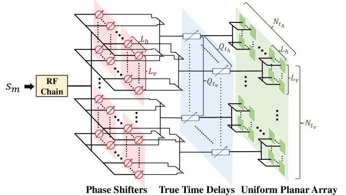
Figure 1: A diagram of hybrid precoding structure in sub-THz systems.

II-A Transmitted Signal

As shown in Fig. 1, we utilize a typical hybrid structure in the sub-THz system, where a small number of TTDs are positioned between the PSs and the antenna array. This setup enables active, frequency-dependent adjustment of phase shifts to effectively deal with beam squint effects. In this architecture, the UPA is divided into $Q_{\text{t}}=Q_{\text{t}_{\text{h}}}\times Q_{\text{t}_{\text{v}}}$ sub-arrays, each of which is connected to a TTD. Each subarray consists of $L=L_{\text{h}}\times L_{\text{v}}$ elements, with $L_{\text{h}}=\frac{N_{\text{t}_{\text{h}}}}{Q_{\text{t}_{\text{h}}}}$ and $L_{\text{v}}=\frac{N_{\text{t}_{\text{v}}}}{Q_{\text{t}_{\text{v}}}}$. The TTDs are also partially connected with the PSs in the same way. Consequently the transmitted signal at the $m$-th subcarrier is

$$\bm{x}_{m}=\sqrt{p_{m}}\bm{F}_{\text{TD},m}\bm{f}_{\text{PS}}s_{m},\vspace{-0.2cm}$$ (1)

where $s_{m}\!\sim\!\mathcal{CN}(0,1)$ is the data symbol for the user at the $m$-th subcarrier. $\bm{p}=[p_{1},\cdots,p_{M}]$ is the transmitting power across subcarriers. $\bm{f}_{\text{PS}}\in\mathbb{C}^{N_{\text{t}}}$ denotes frequency-independent phase shifter (PS) network, with $|\bm{f}_{\text{PS}}[n]|=1$. $\bm{F}_{\text{TD},m}=\text{diag}\left\{\text{vec}\left[e^{j2\pi f_{m}(\bm{T}\otimes\bm{1}^{L_{\text{h}}\times L_{\text{v}}})}\right]\right\}$ denotes the frequency-dependent phase shifts introduced by the TTDs at the $N_{\text{t}}$ antennas, with $\bm{T}\in\mathbb{R}^{Q_{\text{t}_{\text{h}}}\times Q_{\text{t}_{\text{v}}}}$ being the value of delays in TTDs, and $\bm{1}^{L_{\text{h}}\times L_{\text{v}}}$ being the all-one matrix. Taking consideration of the prohibitive cost of arbitrary time delays, finite-value finite-resolution $B_{\text{t}}$-bit TTDs are utilized. i.e.,

$$\bm{T}[q_{h},q_{v}]\in\mathcal{T}\triangleq\left\{\frac{b}{2^{B_{\text{t}}}}t_{\text{max}}|b=0,1,2,\cdots,2^{B_{\text{t}}}-1\right\},\vspace{-0.2cm}$$ (2)

where $q_{h}\in[1,Q_{\text{t}_{\text{h}}}]$, $q_{v}\in[1,Q_{\text{t}_{\text{v}}}]$, and $t_{\text{max}}$ is the maximal achievable time delay determined by the hardware.

II-B Communication Channel

The communication channel between the BS and the user at the $m$-th subcarrier is expressed as

$$\bm{h}_{\text{c},m}=\beta_{\text{c},m}e^{-j2\pi f_{m}\tau_{\text{c}}}\bm{a}_{\text{t}}(\theta_{\text{c}},\phi_{\text{c}},f_{m}),\vspace{-0.2cm}$$ (3)

where $\beta_{\text{c},m}\sim\mathcal{CN}(0,\sigma_{\beta}^{2})$ and $\tau_{\text{c}}\sim\mathcal{U}(0,\tau_{max}]$ are the complex gain and the propagation delay of the line-of-sight (LoS) path. $\theta_{\text{c}}\in[0,\pi]$ and $\phi_{\text{c}}\in[-\pi/2,\pi/2]$ are the elevation and the azimuth angles of the user respectively. $\bm{a}_{\text{t}}(\theta_{\text{c}},\phi_{\text{c}},f_{m})=\bm{a}^{\text{h}}(\theta_{\text{c}},\phi_{\text{c}},f_{m})\otimes\bm{a}^{\text{v}}(\theta_{\text{c}},f_{m})\in\mathbb{C}^{N_{\text{t}}\times 1}$ denotes the steering vector at the $m$-th subcarrier towards $\theta_{\text{c}}$ and $\phi_{\text{c}}$, where $\bm{a}^{\text{h}}(\theta,\!\phi,\!f_{m})[n_{\text{t}_{\text{h}}}]=\frac{1}{\sqrt{N_{\text{t}_{\text{h}}}}}e^{j\pi\!\frac{f_{m}}{f_{\text{c}}}\!\sin\!{\phi}\sin\!{\theta}(n_{\text{t}_{\text{h}}}\!\!-\!\!1)}$ and $\bm{a}^{\text{v}}(\theta,\!f_{m})[n_{\text{t}_{\text{v}}}]=\frac{1}{\sqrt{N_{\text{t}_{\text{v}}}}}e^{j\pi\frac{f_{m}}{f_{\text{c}}}\cos{\theta}(n_{\text{t}_{\text{v}}}-1)}$. Then the received signal at the user at the $m$-th subcarrier is

$$y_{\text{c},m}=\sqrt{p_{m}}\bm{h}_{\text{c},m}^{\text{H}}\bm{F}_{\text{TD},m}\bm{f}_{\text{PS}}s_{m}+n_{\text{c},m},\vspace{-0.2cm}$$ (4)

where $n_{\text{c},m}$ is additive white Gaussian noise with power being $\sigma_{\text{c}}^{2}$. The data rate for the user at the $m$-th subcarrier is

$$R_{\text{c},m}=\log_{2}\left(1+\frac{p_{m}|\bm{h}_{\text{c},m}^{\text{H}}\bm{F}_{\text{TD},m}\bm{f}_{\text{PS}}|^{2}}{\sigma_{\text{c}}^{2}}\right),\vspace{-0.3cm}$$ (5)

and the total rate is $R_{\text{c}}=\sum_{m=1}^{M}R_{\text{c},m}$.

II-C Sensing Channel

The target response matrix at the $m$-th subcarrier $\bm{G}_{m}=\sum_{k=1}^{K}\alpha_{k,m}\bm{a}_{\text{t}}(\theta_{\text{s},k},\phi_{\text{s},k},f_{m})\bm{a}^{\text{T}}_{\text{t}}(\theta_{\text{s},k},\phi_{\text{s},k},f_{m})=\bm{A}_{\text{r},m}\bm{\Sigma}_{m}\bm{A}_{\text{t},m}^{T}$, where $\alpha_{k,m}\sim\mathcal{CN}(0,\sigma_{\alpha}^{2})$ denotes the complex reflection coefficient of the $k$-th target at the $m$-th subcarrier. $\bm{\theta}_{\text{s}}=[\theta_{\text{s},1},\cdots,\theta_{\text{s},K}]$ and $\bm{\phi}_{\text{s}}=[\phi_{\text{s},1},\cdots,\phi_{\text{s},K}]$ denote the elevation and the azimuth angles of the $K$ targets respectively. $\bm{A}_{\text{t},m}=[\bm{a}_{\text{t}}(\theta_{\text{s},1},\phi_{\text{s},1},f_{m}),\cdots,\bm{a}_{\text{t}}(\theta_{\text{s},K},\phi_{\text{s},K},f_{m})]$, and $\Sigma_{m}=\text{diag}(\alpha_{1,m},\cdots,\alpha_{K,m})$. Then the echo at the $m$-th subcarrier at BS can be written as

$$\bm{y}_{\text{s},m}=\sqrt{p_{m}}\bm{A}_{\text{r},m}\bm{\Sigma}_{m}\bm{A}_{\text{t},m}^{T}\bm{F}_{\text{TD},m}\bm{f}_{\text{PS}}s_{m}+\bm{n}_{\text{s},m},\vspace{-0.2cm}$$ (6)

with $\bm{n}_{\text{s},m}\sim\mathcal{CN}(\bm{0},\sigma_{\text{s}}^{2}\bm{I}_{N_{\text{t}}})$ being the ISAC receiver noise. We consider whitening the received noise to enforce adherence to a complex Gaussian distribution. Accordingly, the Fisher information matrix with respect to $\bm{\theta}$ and $\bm{\phi}$ is expressed as

$$\bm{J}_{m}=\frac{2}{\sigma_{\text{s}}^{2}}\text{Re}\left[\begin{matrix}\bm{J}_{m}(\bm{\theta}_{\text{s}},\bm{\theta}_{\text{s}})&\bm{J}_{m}(\bm{\theta}_{\text{s}},\bm{\phi}_{\text{s}})\\ \bm{J}_{m}^{\text{H}}(\bm{\theta}_{\text{s}},\bm{\phi}_{\text{s}})&\bm{J}_{m}(\bm{\phi}_{\text{s}},\bm{\phi}_{\text{s}})\\ \end{matrix}\right],\vspace{-0.2cm}$$ (7)

where

$$\bm{J}_{m}(\bm{\theta},\bm{\phi}) \!=\!(\dot{\bm{A}}_{\text{r},\theta,m}^{\text{H}}\dot{\bm{A}}_{\text{r},\phi,m})\!\odot\!(\bm{\Sigma}_{m}^{*}\bm{A}_{\text{t},m}^{\text{H}}\bm{R}_{x,m}^{*}\bm{A}_{\text{t},m}\bm{\Sigma}_{m})$$

$$+\!(\dot{\bm{A}}_{\text{r},\theta,m}^{\text{H}}\bm{A}_{\text{r},m})\!\odot\!(\bm{\Sigma}_{m}^{*}\bm{A}_{\text{t},m}^{\text{H}}\bm{R}_{x,m}^{*}\dot{\bm{A}}_{\text{t},\phi,m}\bm{\Sigma}_{m})$$

$$+\!(\bm{A}_{\text{r},m}^{\text{H}}\dot{\bm{A}}_{\text{r},\phi,m})\!\odot\!(\bm{\Sigma}_{m}^{*}\dot{\bm{A}}_{\text{t},\theta,m}^{\text{H}}\bm{R}_{x,m}^{*}\bm{A}_{\text{t},m}\bm{\Sigma}_{m})$$

$$+\!(\bm{A}_{\text{r},m}^{\text{H}}\!\bm{A}_{\text{r},m})\!\odot\!(\bm{\Sigma}_{m}^{*}\dot{\bm{A}}_{\text{t},\theta,m}^{\text{H}}\!\bm{R}_{x,m}^{*}\!\dot{\bm{A}}_{\text{t},\phi,m}\bm{\Sigma}_{m}),$$

with $\dot{\bm{A}}_{\text{i},\theta,m}=\left[\frac{\partial\bm{a}_{\text{i}}(\theta_{1},\phi_{1},f_{m})}{\partial\theta_{1}},\cdots,\frac{\partial\bm{a}_{\text{i}}(\theta_{K},\phi_{K},f_{m})}{\partial\theta_{K}}\right]$ and $\dot{\bm{A}}_{\text{i},\phi,m}=\left[\frac{\partial\bm{a}_{\text{i}}(\theta_{1},\phi_{1},f_{m})}{\partial\phi_{1}},\cdots,\frac{\partial\bm{a}_{\text{i}}(\theta_{K},\phi_{K},f_{m})}{\partial\phi_{K}}\right]$ ($\text{i}=\{\text{t},\text{r}\}$), and $\bm{R}_{x,m}=\bm{x}_{m}\bm{x}_{m}^{\text{H}}=p_{m}\bm{F}_{\text{TD},m}\bm{f}_{\text{PS}}\bm{f}_{\text{PS}}^{\text{H}}\bm{F}_{\text{TD},m}^{\text{H}}$ denotes the sampled covariance matrix of $\bm{x}_{m}$. Therefore the Cramér-Rao bound (CRB) associated with angle estimation is calculated as

$$\text{CRB}(\bm{\theta}_{\text{s}},\bm{\phi}_{\text{s}})=\text{Tr}\left((\sum_{m=1}^{M}\bm{J}_{m})^{-1}\right).\vspace{-0.1cm}$$ (8)

II-D Dual-Functional Gain: The Performance Indicator

We define the dual-functional gain as the metric for comprehensively evaluating the performance of both functionalities. Given the communication and sensing channels $\{\bm{h}_{\text{c},m}\}_{m=1}^{M}$ and $\{\bm{G}_{m}\}_{m=1}^{M}$, we characterize the rate-CRB region corresponding to all rate-CRB pairs that can be simultaneously achieved under the total power $P_{\text{t}}$, i.e.,

$$\mathcal{C}^{\text{ISAC}}(P_{\text{t}},\bm{h}_{c},\bm{G})\!\triangleq\!\!\!\bigcup_{\text{T},\bm{f}_{\text{PS}},\bm{p}}\!\!\{(x,y)|x\!\leqslant\!R_{\text{c}},y\!\geqslant\!\text{CRB}(\bm{\theta}_{\text{s}},\!\bm{\phi}_{\text{s}})\}.\vspace{-0.1cm}$$ (9)

Denote $(R_{\text{sen}},\text{CRB}_{\text{min}})$ as the point achieved by the sensing-dedicated scheme and $(R_{\text{max}},\text{CRB}_{\text{com}})$ by the communication-dedicated scheme. Then $\mathcal{C}^{\text{ortho}}(P_{\text{t}},\!\bm{h}_{c},\!\bm{G})$ denotes the achievable region under non-ISAC orthogonal operations, bounded by the line segment between $(R_{\text{sen}},\text{CRB}_{\text{min}})$ and $(R_{\text{max}},\text{CRB}_{\text{com}})$. Then the dual-functional gain can be measured as

$$\varrho=\frac{\int_{(x,y)\in\mathcal{C}^{\text{ISAC}}\backslash\mathcal{C}^{\text{ortho}}}dxdy}{(R_{\text{max}}-R_{\text{sen}})(\text{CRB}_{\text{com}}-\text{CRB}_{\text{min}})/2}\in[0,1),\vspace{-0.1cm}$$ (10)

representing the expansion of the Pareto boundary of $\mathcal{C}^{\text{ISAC}}$ compared to that of $\mathcal{C}^{\text{ortho}}$, where $\backslash$ denotes the difference set. $\varrho=0$ denotes the orthogonal operation and $\varrho\rightarrow 1$ means both $R_{\text{max}}$ and $\text{CRB}_{\text{min}}$ are simultaneously approached. Our objective is to jointly optimize TTDs, PSs and power allocation across subcarriers for maximizing the dual-functional gain.

III SA-Opt: Squint-Aware ISAC Hybrid
Precoding Optimization

In this section, we propose a squint-aware hybrid precoding scheme, SA-Opt, based on the existing sub-THz hardware architecture. Initially, we optimize the TTDs to maximize the correlation between equivalent C-S channels, laying the foundation for dual-functional gain enhancement. Subsequently, we optimize the PSs and power allocation to further approach the Pareto boundary.

III-A Definition of C-S Channel Correlation

Denote $\widehat{\bm{h}}^{\text{b}}_{\text{c}}=\frac{\sum_{m=1}^{M}|\bm{h}^{\text{b}}_{\text{c},m}|}{\|\sum_{m=1}^{M}|\bm{h}^{\text{b}}_{\text{c},m}|\|_{1}}$ and $\widehat{\bm{h}}^{\text{b}}_{\text{s}}=\frac{\sum_{m=1}^{M}|\bm{h}^{\text{b}}_{\text{s},m}|}{\|\sum_{m=1}^{M}|\bm{h}^{\text{b}}_{\text{s},m}|\|_{1}}$ as the normalized beamspace channels across all subcarriers, with $\bm{h}^{\text{b}}_{\text{c},m}=\bm{D}_{\text{t}}^{H}\bm{h}_{\text{c},m}$ and $\bm{h}^{\text{b}}_{\text{s},m}=\text{diag}(\bm{D}_{\text{r}}^{\text{H}}\bm{G}_{m}\bm{D}_{\text{t}})$ being the equivalent beamspace communication and sensing channels. $\bm{D}_{\text{t}}\in\mathbb{C}^{N_{\text{t}}\times G_{\text{t}}}$ and $\bm{D}_{\text{r}}\in\mathbb{C}^{N_{\text{r}}\times G_{\text{t}}}$ are the dictionary uniformly sampled in beamspace [16].

Definition 1.

With the beamspace channels $\widehat{\bm{h}}^{\text{b}}_{\text{c}}$ and $\widehat{\bm{h}}^{\text{b}}_{\text{s}}$ defined, the communication-sensing (C-S) channel correlation is quantified as follows:

$$\text{Cor}(\bm{h}_{\text{c}},\bm{G})=\frac{1}{\text{KL}\{\widehat{\bm{h}}^{\text{b}}_{\text{c}},\widehat{\bm{h}}^{\text{b}}_{\text{s}}\}},\vspace{-0.2cm}$$ (11)

where $\text{KL}(\bm{p},\bm{q})=\sum_{n=1}^{N}p(n)\ln\frac{p(n)}{q(n)}$ denotes the Kullback-Leibler (K-L) divergence.

Proposition 1.

Denote $R^{\star}(P_{\text{t}},\bm{h}_{\text{c}},\bm{G})$ and $\text{CRB}^{\star}(P_{\text{t}},\bm{h}_{\text{c}},\bm{G})$ as a rate-CRB pair on the Pareto boundary of $\mathcal{C}^{\text{ISAC}}(P_{\text{t}},\bm{h}_{c},\bm{G})$. Given $P_{\text{t}}$, both $R^{\star}(P_{\text{t}},\bm{h}_{\text{c}},\bm{G})$ and $(\text{CRB}^{\star}(P_{\text{t}},\bm{h}_{\text{c}},\bm{G}))^{-1}$ increase with higher C-S channel correlation $\text{Cor}(\bm{h}_{\text{c}},\bm{G})$.

Proof.

See Appendix A. ∎

III-B C-S Channel Correlation Maximization through TTDs

Note that TTDs contribute to adjusting the equivalent wideband channels, i.e., $\widetilde{\bm{h}}_{\text{c},m}=\bm{F}_{\text{TD,m}}^{\text{H}}\bm{h}_{\text{c},m}$ and $\widetilde{\bm{G}}_{m}=\bm{G}_{m}\bm{F}_{\text{TD,m}}$. we first design TTDs to maximize the C-S channel correlation by solving

$$\underset{{\bm{T}}}{\max} ~{}\text{Cor}(\widetilde{\bm{h}}_{\text{c}},\widetilde{\bm{G}})$$ (12)

s.t. $$~{}\bm{F}_{\text{TD},m}=\text{diag}\left\{\text{vec}\left[e^{\j 2\pi f_{m}(\bm{T}\otimes\bm{1}^{L_{\text{h}}\times L_{\text{v}}})}\right]\right\},$$ (12a)

$$~{}\bm{T}[q_{\text{h}},q_{\text{v}}]\in\mathcal{T}.\vspace{-0.5cm}$$ (12b)

Since both the objective and the constraints are complicated, we conduct an iterative exhaustive search on $\bm{T}[q_{h},q_{v}]$ in the feasible region $\mathcal{T}$ in an element-wise manner.

III-C Alternating Optimization of $\bm{f}_{\text{PS}}$ and $\bm{p}$

After TTDs are fixed, the PSs and the power allocation across subcarriers are optimized to improve ISAC performance under the adjusted equivalent channels. $\bm{f}_{\text{PS}}$ and $\bm{p}$ are optimized in an alternating manner.

Updating $\bm{f}_{\text{PS}}$:

We first optimize $\bm{f}_{\text{PS}}$ with fixed $\bm{p}_{m}$, for maximizing the antenna array gain at both user and echo reception, which is consistent with the ISAC performance enhancement. The problem is formulated as

$$\underset{{\bm{f}_{\text{PS}}}}{\max}\! ~{}\sum_{m=1}^{M}p_{m}\left[\|\widetilde{\bm{h}}_{\text{c},m}^{\text{H}}\bm{f}_{\text{PS}}\|_{2}^{2}\!+\!\frac{\eta}{N_{\text{r}}}\|\widetilde{\bm{G}}_{\text{s},m}\bm{f}_{\text{PS}}\|_{2}^{2}\right]$$ (13)

s.t. $$~{}|\bm{f}_{\text{PS}}[n]|=1,~{}n\in[1,N_{\text{t}}],\vspace{-0.3cm}$$ (13a)

where $\eta$ is the weighting coefficient to balance array gain for sensing and communications. Using Cauchy-Schwarz inequality for relaxation, a closed-form solution is

$$\bm{f}_{\text{PS}}\!=\!\text{exp}\left[j\angle\left(\sum_{m=1}^{M}\!\sqrt{p_{m}}(\widetilde{\bm{h}}_{\text{c},m}\!+\!\sum_{r=1}^{N_{\text{r}}}\!\frac{\eta}{N_{\text{r}}}\widetilde{\bm{G}}^{\text{H}}_{m}[r,:])\right)\right].\vspace{-0.1cm}$$ (14)

Updating $\bm{p}$:

With $\bm{f}_{\text{PS}}$ updated, power allocation across subcarriers is optimized to minimize the CRB of targets’ angles estimation while ensuring compliance with the user’s communication rate requirements, by solving

$$\underset{{\bm{p}}}{\min} ~{}\text{CRB}(\bm{\theta}_{\text{s}},\bm{\phi}_{\text{s}})$$ (15)

s.t. $$~{}|\overline{h}_{\text{c},m}|^{2}p_{m}\geqslant\Gamma,$$ (15a)

$$~{}\|\bm{p}\|_{1}\leqslant\frac{P_{\text{t}}}{N_{\text{t}}},\vspace{-0.45cm}$$ (15b)

where $\overline{h}_{\text{c},m}=\widetilde{\bm{h}}_{\text{c},m}^{\text{H}}\bm{f}_{\text{PS}}$ is the equivalent digital channel, and $\Gamma$ is SNR threshold at the user. Note that the objective can be relaxed as $\text{Tr}\!\left[(\sum_{m=1}^{M}p_{m}\bm{J}_{m})^{-1}\!\right]\!\!\leqslant\!\frac{1}{M^{2}}\!\sum_{m=1}^{M}\frac{1}{p_{m}}\text{Tr}(\bm{J}_{m}^{-1})$ via Jensen’s inequality, giving rise to

$$\underset{{\bm{p}}}{\min} ~{}\text{Tr}\left(\bm{Q}(\text{diag}(\bm{p}))^{-1}\right)$$ (16)

s.t. $$~{}(\ref{Problem4_a}),(\ref{Problem4_b}),\vspace{-0.3cm}$$

where $\bm{Q}=\text{diag}([\text{Tr}(\bm{J}_{1}^{-1}),\cdots,\text{Tr}(\bm{J}_{M}^{-1})])$. This problem is a convex programming and can be solved by CVX.

Algorithm 1 Squint-Aware Optimization-Based ISAC Hybrid Precoding (SA-Opt)

Input:$\{\bm{h}_{\text{c},m}\}_{m=1}^{M}$, $\{\bm{G}_{m}\}_{m=1}^{M}$, $M$, $N_{\text{t}}$, $N_{\text{r}}$, $Q_{\text{t}_{\text{h}}}$, $Q_{\text{t}_{\text{v}}}$, $P_{\text{t}}$, $\eta$, $\Gamma$, $\sigma_{\text{c}}$, $\sigma_{\text{s}}$, $N_{\text{iter}}$, $N_{\text{AO}}$;
Output:$\bm{T},\bm{F}_{\text{RF}}$ and $\bm{p}$;
Steps:

1:Initialize $\bm{T}$ and $\bm{f}_{\text{PS}}$ randomly, initialize $\bm{p}=\frac{P_{\text{t}}}{N_{\text{t}}M}\bm{1}$;

2:for $n=1$ to $N_{\text{iter}}$ do

3:     for $q_{\text{h}}=1$ to $Q_{\text{t}_{\text{h}}}$ do

4:         for $q_{\text{v}}=1$ to $Q_{\text{t}_{\text{v}}}$ do

5:              Set $\bm{T}[q_{\text{h}},\!q_{\text{v}}]\!\!=\!\!\mathop{\arg\!\min}\limits_{t\in\mathcal{T}}\!\text{Cor}(\bm{h}_{\text{c}},\!\bm{G}_{\text{s}};\!\bm{T}[q_{\text{h}},\!q_{\text{v}}]\!\!=\!\!t)$;               

6:for $n=1$ to $N_{\text{AO}}$ do

7:     Update $\bm{f}_{\text{PS}}$ as (14);

8:     Update $\bm{p}$ by solving (16);

IV CSP-Net: Low-complexity squint-aware
ISAC hybrid precoding

The proposed SA-Opt exhibits high computational complexity due to its exhaustive search and iterative processes. Therefore, in this section, we present a low-complexity alternative based on unsupervised learning, termed as the complex-valued squint-aware hybrid precoding network (CSP-Net).

IV-A Complex-valued Network Structure

We employ a complex-valued neural network architecture tailored for complex channels, mainly including complex-valued convolutional layers, complex-valued fully-connected (FC) layers, complex-valued batch normalization (BN) layers, and complex-valued activation functions, as detailed in [17].

The input contains the communication and sensing channels $\{\bm{h}_{\text{c},m},\bm{G}_{m}\}_{m=1}^{M}$. We pre-process the channel data as $\overline{\bm{H}}_{m}=\bm{h}_{\text{c},m}\bm{h}_{\text{c},m}^{\text{H}}$ and $\overline{\bm{G}}_{m}=\bm{G}_{m}$ respectively. Then the total data are represented as $\overline{\bm{H}}=\{\overline{\bm{H}}_{m}\}_{m=1}^{M}\in\mathbb{C}^{M\times N_{\text{t}}\times N_{\text{t}}}$ and $\overline{\bm{G}}=\{\overline{\bm{G}}_{m}\}_{m=1}^{M}\in\mathbb{C}^{M\times N_{\text{r}}\times N_{\text{t}}}$. Following this, we perform power normalization before inputting them into the neural network.

IV-B Layer Description

The proposed CSP-Net consists of four parts: Communication channel feature extraction network (CFE-Net), sensing channel feature extraction network (SFE-Net), fusion layer (FL) and parameter design network (PD-Net). The detailed architecture design of CSP-Net is illustrated in Fig. 2.

IV-B1 CFE-Net & SFE-Net

The features from the communication and sensing channels are extracted respectively by CFE-Net and SFE-Net. For communication channel data $\bm{H}_{\text{in}}$, two layers of complex convolutional blocks are employed, each of which includes one complex convolutional layer, one complex ReLU, one complex batch normalization (BN) and one complex pooling. Similarly, another branch of convolutional blocks is employed for $\bm{G}_{\text{in}}$ in SFE-Net. Parameterized by $\phi_{\text{CFE}}$ and $\phi_{\text{SFE}}$, the outputs are represented as $\bm{V}_{\text{c}}=\phi_{\text{CFE}}(\bm{H}_{\text{in}})$ and $\bm{V}_{\text{s}}=\phi_{\text{SFE}}(\bm{G}_{\text{in}})$ respectively.

IV-B2 Fusion Layer

To further enhance the features from $\bm{H}_{\text{in}}$ and $\bm{G}_{\text{in}}$ and extract the correlation between them, we tailor the convolutional block attention module (CBAM) in [18] on $[\bm{V}_{\text{c}},\bm{V}_{\text{s}}]$ with the complex-valued network, including a channel-based attention and a spatial-based attention. Then the output is flattened as $\bm{v}$ for the following precoding design.

IV-B3 PD-Net

The values of TTDs, PSs and power allocation are sequentially predicted through PD-Net. Two complex FC layers are first employed to predict the value of TTDs, with complex ReLU and complex sigmoid functions as the activation functions. However, the output, $\hat{\bm{t}}\in[0,1]^{Q_{\text{t}}}$, fails to satisfy the finite-resolution constraint. Therefore the post-processing is conducted to project $\hat{\bm{t}}$ into the feasible region as $\bm{T}_{\text{out}}=\mathcal{Q}(\text{reshape}(t_{\text{max}}\hat{\bm{t}}))$, where $\mathcal{Q}(\bm{T}[q_{\text{h}},q_{\text{v}}])=\mathop{\arg\min}\limits_{t\in\mathcal{T}}\|t-\bm{T}[q_{\text{h}},q_{\text{v}}]\|_{2}^{2}$. Concatenating $\bm{v}$ and $\hat{\bm{t}}$ as the input of the following network, we proceed to predict the PSs through one complex FC layer, and the output is expressed as $\hat{\bm{\varphi}}\in[0,1]^{N_{\text{t}}}$. Then PSs are calculated as $\bm{\varphi}_{\text{out}}=2\pi\hat{\bm{\varphi}}$. Since the design of power allocation is determined by both the channels and the configuration of analog parts, we concatenate $\bm{v}$, $\hat{\bm{t}}$ and $\hat{\bm{\varphi}}$ to predict $\bm{p}$ using another complex FC layer.

The overall parameters in the proposed CSP-Net are $\phi_{\text{CSP}}=\{\phi_{\text{CFE}},\phi_{\text{SFE}},\phi_{\text{FL}},\phi_{\text{PD}}\}$.

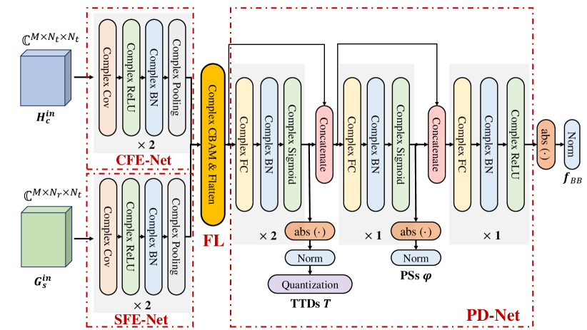
Figure 2: The architecture of CSP-Net.

IV-C Loss Function

We employ an unsupervised learning-based method for the model training. To achieve the goal of maximizing ISAC utility with the awareness of the C-S correlation, we customize the loss function for the $i$-th sample in the batch as

$$L(\phi_{\text{CSP}})\!\!=\!\!-\frac{1}{N_{\text{b}}}\!\!\sum_{i=1}^{N_{\text{b}}}\!\!\frac{\text{Cor}(\bm{h}_{\text{c}}^{(i)},\!\bm{G}^{(i)};\bm{T}^{(i)})}{\text{Cor}^{\star}(\bm{h}_{\text{c}}^{(i)},\!\bm{G}^{(i)};\bm{T}^{(i)})}\!\!\left[\!\!\frac{R_{\text{c}}^{(i)}}{R_{\text{max}}^{(i)}}\!\!+\!\!\frac{\text{CRB}_{\text{min}}^{(i)}}{\text{CRB}^{(i)}}\!\right],\vspace{-0.1cm}$$ (17)

with $N_{\text{b}}$ denoting the batch size. In offline training stage, CSP-Net is updated with this loss function by back propagation in randomly-sampled batches. In the deployment, the channel data are input to the well-trained CSP-Net, and the values of TTDs, PSs and power allocation are obtained sequentially.

V Benchmark scheme: Controlled beam squint

To verify the effectiveness of proposed squint-aware methods, we further develop a benchmark scheme that directly controls beam squint for ISAC without correlation adjustment.

V-1 Analog precoding design

Denote $\{\bm{F}_{m}^{\star}\}_{m=1}^{M}$ as the ideal frequency-dependent analog precoding matrices, making the beams at all subcarriers point to the desired directions $\{(\theta_{m}^{\star},\phi_{m}^{\star})\}_{m=1}^{M}$ to guarantee the coverage of both targets and users. To achieve the ideal array gain, the precoder at $f_{m}$ is set as the steering vector towards ($\theta_{m}^{\star},\phi_{m}^{\star}$), i.e., $\bm{F}_{m}^{\star}=\bm{a}_{\text{t}}(\theta_{m}^{\star},\phi_{m}^{\star},f_{m})$. Subsequently, $\bm{T}$ and $\bm{f}_{\text{PS}}$ are jointly designed to approximate $\bm{F}_{m}^{\star}$ by solving

$$\underset{{\bm{T},\bm{\varphi}}}{\min} ~{}\frac{1}{M}\sum_{m=1}^{M}\|\bm{F}_{\text{TD},m}\bm{f}_{\text{PS}}-\bm{F}_{m}^{\star}\|_{\text{F}}^{2}$$ (18)

s.t. $$~{}(\ref{Problem1_a}),(\ref{Problem1_b}),(\ref{Problem2_a}).\vspace{-0.35cm}$$

According to [19], this problem can be equivalently transformed into a convex one as

$$\underset{{\bm{\varphi},\bm{T}}}{\min} \frac{1}{M}\!\!\sum_{m=1}^{M}\!\sum_{q_{\text{h}}=1}^{Q_{\text{t}_{\text{h}}}}\!\sum_{q_{\text{v}}=1}^{Q_{\text{t}_{\text{v}}}}\!\sum_{l_{\text{h}}=1}^{L_{\text{h}}}\!\sum_{l_{\text{v}}=1}^{L_{\text{v}}}\!|\bm{\varphi}[(q_{\text{h}}\!-\!1\!)L_{\text{h}}\!\!+\!\!l_{\text{h}},\!(q_{\text{v}}\!\!-\!\!1)L_{\text{v}}\!\!+\!\!l_{\text{v}}]\!$$

$$-\!2f_{m}\bm{T}[q_{\text{h}},\!q_{\text{v}}]\!+\!\frac{f_{m}}{f_{\text{c}}}[\sin{\theta_{m}}\sin{\phi_{m}}((q_{\text{h}}\!-\!1)L_{\text{h}}\!+\!l_{\text{h}}\!-\!1)$$

$$+\!\cos{\theta_{m}}((q_{\text{v}}\!-\!1)L_{\text{v}}\!+\!l_{\text{v}}\!-\!1)]|^{2}$$ (19)

s.t. $$~{}0\leqslant\bm{T}[q_{\text{h}},q_{\text{v}}]\leqslant t_{\text{max}},$$ (19a)

$$~{}\bm{f}_{\text{PS}}=e^{j\bm{\varphi}},\vspace{-0.3cm}$$ (19b)

and solved by the off-the-shelf toolbox. $\bm{T}$ is then quantized to meet the finite-resolution constraint.

V-2 Power allocation

The remaining task is to optimize $\bm{p}$ with $\bm{T}$ and $\bm{\varphi}$ fixed, as detailed in Section III-C.

VI Simulation Results

In this section, simulation results are presented to evaluate the performance of the proposed schemes. Unless otherwise specified, the transceiver-related parameters are set as: $N_{\text{t}_{\text{h}}}=N_{\text{t}_{\text{v}}}=16$, $N_{\text{t}}=256$, $N_{\text{r}}=256$, $Q_{\text{t}_{\text{h}}}=Q_{\text{t}_{\text{v}}}=8$, $L_{\text{h}}=L_{\text{v}}=2$. The central frequency point is $f_{\text{c}}=100$ GHz, with $B=8$ GHz and $M=32$. $t_{\text{max}}=100$ ps and $B_{\text{t}}=4$. The channel related parameters are: $\sigma_{\beta}=1$, $\sigma_{\alpha}=0.6$, $\tau_{\text{max}}=100$ ns. $K=3$. The noise variances are $\sigma_{\text{c}}^{2}=\sigma_{\text{s}}^{2}=0$ dBm. SNR is defined as $\frac{P_{\text{t}}}{\sigma_{\text{c}}^{2}}$. We define the mean squared interval of angle (MSIA) between targets and the user as $\sqrt{\frac{\sum_{k=1}^{K}(\theta_{\text{s},k}-\theta_{\text{c}})^{2}+(\phi_{\text{s},k}-\phi_{\text{c}})^{2}}{2K}}$. The methods to be evaluated include:

• SA-Opt: The proposed optimization based approach.

• CSP-Net: The proposed learning-aided scheme.

• CBS-ISAC: Controlling beam squint for ISAC coverage.

• Opt w/o TTD: Alternating optimization without TTDs.

• Com-dedicated: Focusing beams to the user.

• Sensing-dedicated: Spreading beams to cover targets.

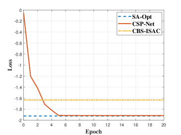
(a) Loss function.

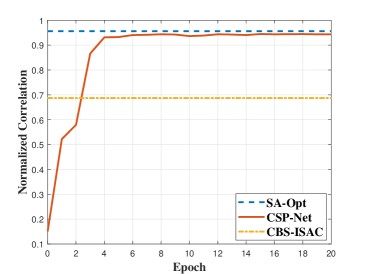
(b) Normalized correlation.

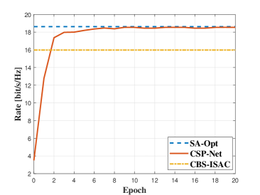
(c) Rate.

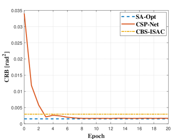
(d) CRB.

Figure 3: Loss and performance versus training epochs.

TABLE I: Ablation Experiments in CSP-Net

	Loss	Correlation	Rate	CRB
CSP-Net	-1.915	0.9443	18.52	0.00154
real-valued	-1.802	0.9167	18.34	0.00168
w/o CBAM	-1.878	0.9388	18.37	0.00158

We first validate the training process of the proposed CSP-Net. The overall loss decreases significantly during training and converges after around 10 epochs. Since the correlation is included in the customized loss function, the C-S channel correlation increases significantly, beneficial to improvement of C-S performance. Through the comparison of the ablation experiments in Table. I, the advantages of the complex-valued neural network and CBAM in processing channel data and integrating channel features can be verified respectively.

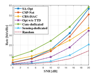
(a) Rate versus SNR.

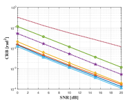
(b) CRB versus SNR.

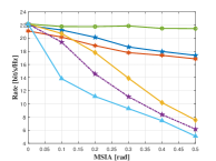
(c) Rate versus MSIA.

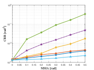
(d) CRB versus MSIA.

Figure 4: ISAC performance comparison.

We then compare the ISAC performance of different schemes in Fig. 4(a) and Fig. 4(b), under MSIA= 0.1. For communications, SA-Opt outperforms the CBS benchmark at high SNR with a gain of 2 dB, approaching the communication-dedicated scheme with perfect alignment for the user. In terms of sensing, the CRB of SA-Opt also outperforms CBS with a gain of 1.5 dB and approaches the sensing-dedicated scheme. This can be attributed to the increased C-S channel correlation, which enhances the multiplexing of resources for both functions. Furthermore, the significance of TTDs in tuning this correlation is evident when compared to the optimization without TTDs. It is worth noting that CSP-Net also outperforms existing benchmarks, approaching SA-Opt.

Furthermore, we compare these schemes under different user-target spatial distributions in Fig. 4(c) and Fig. 4(d), fixing SNR as 10 dB. Due to the limited dispersion of beam squint, the array gain decreases as the user-target angular separation increases, and ISAC performance of benchmarks deteriorate drastically. However, the proposed schemes effectively counteract the performance loss by actively tuning the channels, suggesting a better adaptation to the spatial distribution.

TABLE II: Complexity comparison

Method	Complexity
SA-Opt	$\mathcal{O}(N_{\text{iter}}Q_{\text{t}}2^{B_{\text{t}}}(N_{\text{t}}^{3}N_{\text{r}}^{3}\!+\!2N_{\text{t}}^{2}N_{\text{r}}+2N_{\text{t}}^{2})\!+\!N_{\text{AO}}(M((2K)^{3}\!+\!12N_{\text{t}}^{2}K^{4})\!+\!M^{3}\log{1/\epsilon})$
CSP-Net	$\mathcal{O}(M^{2}(N_{\text{t}}^{2}+N_{\text{t}}N_{\text{r}})+Q_{\text{t}}^{2}+N_{\text{t}}^{2}+M^{2})$
CBS-ISAC	$\mathcal{O}(N_{\text{iter}}(N_{\text{t}}^{3}+Q_{\text{t}}^{3})\log{1/\epsilon})$
Opt w/o TTD	$\mathcal{O}(N_{\text{AO}}(M((2K)^{3}\!+\!12N_{\text{t}}^{2}K^{4})\!+\!M^{3}\log{1/\epsilon}))$

By comparing the ISAC performance boundaries achieved through these methods at SNR=10 dB in Fig. 5(a), we validate the proposed schemes’ effectiveness in enhancing dual-functional gain across different spatial distributions. The complexity of these approaches are analyzed in Table. II, and the running time is compared in Fig. 5(b). SA-Opt achieves the best ISAC performance among the methods at the cost of high complexity, while CSP-Net significantly reduces the complexity to be merely squared with $N_{t}$ and $M$, without a noticeable loss in performance. Therefore SA-Opt is well-suited for quasi-static environments, whereas CSP-Net is more effective in time-varying channels.

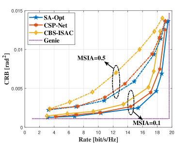
(a) ISAC performance boundaries.

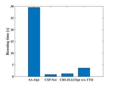
(b) Running time comparison.

Figure 5: Dual-functional gain & running time comparison.

VII Conclusion

In this paper, we proposed two ISAC hybrid precoding approaches for sub-THz systems that incorporate communication-sensing channel correlation adaptation. Firstly we introduced a correlation metric specifically designed for ISAC, followed by optimizing the metric to guide ISAC precoding. Additionally we presented a learning-aided low-complexity alternative, CSP-Net. The proposed schemes effectively enhance the dual-functional gain and demonstrate robustness across various spatial distributions, highlighting the significant impact of C-S channel correlation on performance boundaries. Furthermore, these schemes are compatible with the existing hardware architectures, offering promising applications in sub-THz systems.

Appendix A Proof of the Proposition 1

According to [10], the optimal $\bm{R}_{x,m}$ can be expressed as

$$\bm{R}_{x,m}^{\star}=\bm{U}_{m}\Lambda_{m}\bm{U}_{m}^{\text{H}},\vspace{-0.2cm}$$ (20)

where $\bm{U}_{m}\!=\![\bm{A}_{\text{t},m}^{*},\dot{\bm{A}}_{\text{t},\theta,m}^{*},\dot{\bm{A}}_{\text{t},\phi,m}^{*},\bm{a}_{\text{t}}(\theta_{\text{c}},\phi_{\text{c}},f_{m})]\!=\![\bm{u}_{m,1},\cdots,\!\bm{u}_{m,N_{\text{R}}}]\!\in\!\mathbb{C}^{N_{\text{t}}\times N_{\text{R}}}$ ($N_{\text{R}}\!=\!3K\!+\!1$) serving as the basis vectors under the given C-S channels $\bm{h}_{c}$ and $\bm{G}$, and $\bm{\Lambda}_{m}$ is positive semi-definite with $\bm{\Lambda}_{m}[n_{1},n_{2}]=\lambda_{m,n_{1},n_{2}}$. Then the achievable rate-CRB on the Pareto boundary is written as

$$\bm{R}_{\text{c}}^{\star}=\sum_{m=1}^{M}\log_{2}\left[1+\frac{1}{\sigma_{c}^{2}}\sum_{n_{1}=1}^{N_{\text{R}}}\sum_{n_{2}=1}^{N_{\text{R}}}\lambda_{n_{1},n_{2}}\bm{\Xi}_{\text{c},m}[n_{1},n_{2}]\right],$$

$$\text{CRB}^{\star}\approx N_{\text{R}}^{2}\left[\sum_{n_{1}}^{N_{\text{R}}}\sum_{n_{2}}^{N_{\text{R}}}\lambda_{n_{1},n_{2}}\bm{\Xi}_{\text{s},m}[n_{1},n_{2}]\right]^{-1},\vspace{-0.6cm}$$ (21)

$\bm{\Xi}_{\text{c},m}[n_{1},\!n_{2}]\!=\!\xi_{\text{c},m,n_{1},n_{2}}={\bm{h}_{\text{c},m}^{\text{b}}}^{\text{H}}\bm{D}_{\text{t}}^{\text{H}}\bm{u}_{m,n_{1}}\bm{u}_{m,n_{2}}^{\text{H}}\bm{D}_{\text{t}}\bm{h}_{\text{c},m}^{\text{b}}$, $\bm{\Xi}_{\text{s},m}[n_{1},n_{2}]=\xi_{\text{s},m,n_{1},n_{2}}=\bm{u}_{m,n_{1}}^{\text{H}}\bm{A}_{\text{t},m}\bm{\Sigma}_{m}\bm{\Sigma}_{m}^{*}\bm{A}_{\text{t},m}^{\text{H}}\bm{u}_{m,n_{2}}$ are both determined by the channels. By solving this multi-objective optimization, the optimal $\bm{\Lambda}_{m}$ can be written as

$$\bm{\Lambda}_{m}^{\star}=(\bm{\Xi}_{\text{c},m}+\gamma\bm{\Xi}_{\text{s},m})\frac{\sqrt{P_{\text{t}}}}{\|\bm{\Xi}_{\text{c},m}+\gamma\bm{\Xi}_{\text{s},m}\|_{\text{F}}}.\vspace{-0.15cm}$$ (22)

By substituting (22) into (21), the rate and CRB at Pareto optimum can be described via $\bm{\Xi}_{\text{c},m}$ and $\bm{\Xi}_{\text{s},m}$ as

$$\bm{R}_{\text{c}}^{\star}\!\!=\!\!\log_{2}\!\!\left(\!1\!\!+\!\!\frac{1}{\sigma_{\text{c}}^{2}}\!\!\sum_{n_{1}}^{N_{\text{R}}}\!\!\sum_{n_{2}}^{N_{\text{R}}}\!\!\frac{\sqrt{P_{\text{t}}}(\xi_{\text{c},m,n_{1},\!n_{2}}^{2}\!+\!\!\gamma\xi_{\text{s},m,n_{1},n_{2}}\xi_{\text{c},m,n_{1},n_{2}})}{\|\bm{\Xi}_{\text{c}}\!+\!\gamma\bm{\Xi}_{\text{s}}\|_{\text{F}}}\!\!\right)\!,$$

$$\text{CRB}^{\star}\!\!=\!\!N_{\text{R}}^{2}\!\!\left(\!\sum_{n_{1}}^{N_{\text{R}}}\!\sum_{n_{2}}^{N_{\text{R}}}\frac{\sqrt{P_{\text{t}}}(\gamma\xi_{\text{s},m,n_{1},\!n_{2}}^{2}\!\!+\!\!\xi_{\text{s},m,n_{1},n_{2}}\xi_{\text{c},m,n_{1},n_{2}})}{\|\bm{\Xi}_{\text{c}}\!+\!\gamma\bm{\Xi}_{\text{s}}\|_{\text{F}}}\!\right)^{-1}.$$

Leveraging the sparsity of beamspace channels [16], we denote the indices of peaks in $\widehat{\bm{h}}_{\text{c}}^{\text{b}}$ and $\widehat{\bm{h}}_{\text{s}}^{\text{b}}$ as $\{\psi_{\text{c},m}\}$ and $\{\psi_{\text{s},k,m}\}$. The similarity of these peaks is defined as $\mathcal{S}_{m}(\bm{h}_{\text{c}},\bm{G})=\sum_{k=1}^{K}\mathbb{I}(\psi_{\text{c},m}=\psi_{\text{s},k,m})$ and $\mathcal{S}(\bm{h}_{\text{c}},\bm{G})=\sum_{m=1}^{M}\mathcal{S}_{m}$ with $\mathbb{I}(\cdot)$ being the indicator function. It can be proved that a higher $\text{Cor}(\bm{h}_{\text{c}},\bm{G})$ gives rise to a higher $\mathcal{S}(\bm{h}_{\text{c}},\bm{G})$ [20]. As derived in (23), as $\mathcal{S}(\bm{h}_{\text{c}},\bm{G})$ increases, both $\xi_{\text{c},m,n_{1},n_{2}}$ and $\xi_{\text{s},m,n_{1},n_{2}}$ improve, leading to an increase in $R_{\text{c}}^{\star}$ and a reduction in $\text{CRB}^{\star}$ along the Pareto boundary. Therefore a higher C-S channel correlation improves the dual-functional gain.

$$\xi_{\text{c},m,n_{1},n_{2}}\! \!\approx\!\mathbb{I}(n_{1}\!=\!n_{2}\!=\!\!N_{\text{R}})\!+\!\!2\mathbb{I}(1\!\!\leqslant\!\!n_{1}\!\!\leqslant\!K,\!n_{2}\!\!=\!\!N_{\text{R}})\!\!\sum_{k=1}^{K}\!\mathbb{I}(\psi_{\text{s},k,m}\!\!=\!\!\psi_{\text{c},m})\!+\!\!\mathbb{I}(1\!\!\leqslant\!\!n_{1},\!n_{2}\!\!\leqslant\!\!K)\sum_{k_{1}}^{K}\!\!\sum_{k_{2}}^{K}\!\mathbb{I}(\psi_{\text{s},k_{1},m}\!\!=\!\!\psi_{\text{c},m})\mathbb{I}(\psi_{\text{s},k_{2},m}\!\!=\!\!\psi_{\text{c},m}),$$

$$\vspace{-0.99cm}\xi_{\text{s},m,n_{1},n_{2}}\! \!\approx\!\mathbb{I}(n_{1}\!=\!n_{2}\!=\!\!N_{\text{R}})\sum_{k=1}^{K}\mathbb{I}(\psi_{\text{c},m}\!\!=\!\!\psi_{\text{s},k,m})|\bm{\Sigma}_{m}[k,k]|^{2}\!+\!\mathbb{I}(1\leqslant n_{1},\!n_{2}\!\leqslant\!K)\sum_{k=1}^{K}|\bm{\Sigma}_{m}[k,k]|^{2}.$$ (23)

References

• [1] X. Cheng, D. Duan, S. Gao, and L. Yang, “Integrated sensing and communications (ISAC) for vehicular communication networks (VCN),” IEEE Internet Things J., vol. 9, no. 23, pp. 23 441–23 451, Dec. 2022.
• [2] F. Liu et al., “Integrated sensing and communications: Towards dual-functional wireless networks for 6G and beyond,” IEEE J. Select. Areas Commun., vol. 40, no. 6, pp. 1728–1767, Jun. 2022.
• [3] X. Cheng et al., “Intelligent multi-modal sensing-communication integration: Synesthesia of machines,” IEEE Commun. Surveys Tuts., vol. 26, no. 1, pp. 258–301, 1st Quart. 2024.
• [4] Y. Fan, S. Gao, X. Cheng, L. Yang, and N. Wang, “Wideband generalized beamspace modulation (wGBM) for mmwave massive MIMO over doubly-selective channels,” IEEE Trans. Veh. Technol., vol. 70, no. 7, pp. 6869–6880, Jul. 2021.
• [5] B. Wang, F. Gao, S. Jin, H. Lin, and G. Y. Li, “Spatial- and frequency-wideband effects in millimeter-wave massive MIMO systems,” IEEE Trans. Signal Process., vol. 66, no. 13, pp. 3393–3406, Jul. 2018.
• [6] L. Dai, J. Tan, Z. Chen, and H. V. Poor, “Delay-phase precoding for wideband THz massive MIMO,” IEEE Trans. Wireless Commun., vol. 21, no. 9, pp. 7271–7286, Sept. 2022.
• [7] F. Gao, L. Xu, and S. Ma, “Integrated sensing and communications with joint beam-squint and beam-split for mmWave/THz massive MIMO,” IEEE Trans. Commun., vol. 71, no. 5, pp. 2963–2976, May 2023.
• [8] H. Luo, F. Gao, H. Lin, S. Ma, and H. V. Poor, “YOLO: An efficient terahertz band integrated sensing and communications scheme with beam squint,” IEEE Trans. Wireless Commun., vol. 23, no. 8, pp. 9389–9403, Aug. 2024.
• [9] Y. Liu et al., “Information-theoretic limits of integrated sensing and communication with correlated sensing and channel states for vehicular networks,” IEEE Trans. Veh. Technol., vol. 71, no. 9, pp. 10 161–10 166, Sept. 2022.
• [10] S. Lu, X. Meng, Z. Du, Y. Xiong, and F. Liu, “On the performance gain of integrated sensing and communications: A subspace correlation perspective,” in IEEE International Conference on Communications, 2023, pp. 2735–2740.
• [11] Y. Liu, J. Zhang, Y. Zhang, Z. Yuan, and G. Liu, “A shared cluster-based stochastic channel model for integrated sensing and communication systems,” IEEE Trans. Veh. Technol., vol. 73, no. 5, pp. 6032–6044, May 2024.
• [12] X. Meng, F. Liu, S. Lu, S. P. Chepuri, and C. Masouros, “RIS-assisted integrated sensing and communications: A subspace rotation approach,” in 2023 IEEE Radar Conference (RadarConf23), 2023, pp. 1–6.
• [13] J. Ye, L. Huang, Z. Chen, P. Zhang, and M. Rihan, “Unsupervised learning for joint beamforming design in RIS-aided ISAC systems,” IEEE Wireless Commun. Lett., vol. 13, no. 8, pp. 2100–2104, Aug. 2024.
• [14] A. M. Elbir, K. V. Mishra, and S. Chatzinotas, “Terahertz-band joint ultra-massive mimo radar-communications: Model-based and model-free hybrid beamforming,” IEEE J. Sel. Topics Signal Process., vol. 15, no. 6, pp. 1468–1483, Nov. 2021.
• [15] R. P. Sankar, S. S. Nair, S. Doshi, and S. P. Chepuri, “Learning to precode for integrated sensing and communication systems,” in 2023 31st European Signal Processing Conference (EUSIPCO), 2023, pp. 695–699.
• [16] S. Gao, X. Cheng, and L. Yang, “Mutual information maximizing wideband multi-user (wMU) mmwave massive MIMO,” IEEE Trans. Commun., vol. 69, no. 5, pp. 3067–3078, May 2021.
• [17] C. Trabelsi et al., “Deep complex networks,” 2017, arXiv:2405.14347.
• [18] S. Woo, J. Park, J.-Y. Lee, and I. S. Kweon, “CBAM: Convolutional block attention module,” in Computer Vision – ECCV 2018, 2018, pp. 3–19.
• [19] D. Q. Nguyen and T. Kim, “Joint delay-phase precoding under true-time delay constraints in wideband sub-THz hybrid massive MIMO systems,” IEEE Trans. Commun., vol. 72, no. 10, pp. 6633–6646, Oct. 2024.
• [20] J. R. Hershey and P. A. Olsen, “Approximating the Kullback Leibler divergence between gaussian mixture models,” in IEEE International Conference on Acoustics, Speech and Signal Processing - ICASSP 2007, vol. 4, 2007, pp. 317–320.