A simple way to reduce the number of contours
in the multi-fold Mellin-Barnes integrals

Mauricio Diaz^(a), Ivan Gonzalez ^(b,c) , Igor Kondrashuk ^(c,d),
Eduardo A. Notte-Cuello ^(c,e)
(a) Departamento de Física, Universidad del Bío-Bío, Av. Collao 1202, Casilla 15-C, Concepción, Chile

(b) Instituto de Física y Astronomía, Universidad de Valparaíso,
Av. Gran Bretaña 1111, Valparaíso, Chile

(c) Centro de Ciencias Exactas, Universidad del Bío-Bío, Campus Fernando May,
Av. Andres Bello 720, Casilla 447, Chillán, Chile

(d) Grupo de Matemática Aplicada & Grupo de Física de Altas Energías,
Departamento de Ciencias Básicas, Universidad del Bío-Bío, Campus Fernando May,
Av. Andres Bello 720, Casilla 447, Chillán, Chile

(e) Departamento de Matemáticas, Facultad de Ciencias, Universidad de La Serena,
Av. Cisternas 1200, La Serena, Chile

Mellin-Barnes integral representation of one-loop off-shell box massless diagram is five-fold by construction. On the other hand, it is known from the year 1992 that it may be reduced to certain two-fold MB integral. We propose a way to reduce the number of the MB integration contours from five to two by using the MB integral representation only in combination with basic methods of mathematical analysis such as analytical regularization. We do not use any Barnes lemma to prove the reduction but we use the integral Cauchy formula instead. We recover first the well-known two-fold MB representation for the one-loop triangle massless diagram and then show how the five-fold MB integral representation of one-loop box diagram with all the indices 1 in four spacetime dimensions may be reduced to the two-fold MB representation for one-loop triangle diagram. Singular integrals over Feynman parameters appear in the integrand of the five-fold MB integral representation at the intermediate step. Such integrals should be treated as distributions with respect to certain linear combinations of the initial MB integration variables in the MB integrands. These distributions may be integrated out with a finite number of residues in the limit of removing the analytical regularization. We explain how to apply this strategy to an arbitrary Feynman diagram in order to reduce the number of MB integration contours.
Keywords: Mellin-Barnes transformation, one-loop off-shell massless box diagram, distributions
MSC Classification: 44A15; 44A20; 81T18; 81Q30; 81T13; 33B15; 30E20

1 Introduction

Significant progress has been made in theoretical particle physics with purpose to study scattering amplitudes. Major progress occurred after the BDS conjecture [1, 2] for the amplitudes of four particle processes in maximally symmetric ${\cal N}=4$ SYM theory. However, comparatively fewer studies have focused on Green functions, the quantities obtained from the path integral when expressed in terms of external sources. The first results were obtained by Usyukina and Davydychev [3, 4] in the context of massless ladder diagrams, where they found expressions in terms of polylogarithms and demonstrated the equivalence of three-point and four-point Green functions using a combination of Feynman parameters, Mellin-Barnes integral representations, and the uniqueness trick. The equivalence between four-point and three-point ladder diagrams may also be demonstrated via the Jacobian of a conformal transformation in an auxiliary space dual to the four-dimensional momentum space [5, 6, 7, 8]. Usyukina and Davydychev’s results were based on the loop reduction technique proposed by Belokurov and Usyukina in 1983 for the four-dimensional case [9]. This loop reduction technique was generalized for non-integer dimensions in [10] and [11] by two of us, although this was specifically the case for conformal ladders, which is not a practical case because the index had to be modified to make the Belokurov-Usyukina loop reduction technique applicable when the dimension of spacetime is arbitrary.

The three-point and four-point ladders contribute to the Green functions of rank three and four, respectively. The Green functions can be obtained from the path integral, the logarithm of which is related to the effective action by a Legendre transformation [12]. The path integral and the effective action are restricted by the Slavnov-Taylor identity [12]. In [13], it was shown that the effective action of the dressed mean fields can be treated as the classical action but with the indices of the dressing function depending on two complex variables. These two complex indices are integrated with a function of two complex variables, which determines the auxiliary double ghost vertex in the Landau gauge. This complex function of two variables can be determined by Bethe-Salpeter equation [14, 13]. There is a reason to expect an iterative structure for this complex function of two variables that solves the BS equation.

The reason for the simple iterative structure of this double ghost vertex is that the structure of the three-gluon vertex in ${\cal N}=4$ SYM theory is fixed by conformal invariance in the Landau gauge [15, 16, 17, 19]. This simple structure is mapped onto the structure of the $Lcc$ vertex by the ST identity, which cannot be fixed by conformal invariance because the auxiliary field $L$ does not appear in the integration measure of the path integral [17]. Despite this, the structure of the double ghost vertex is expected to remain simple at all loops because the the structure of the three gluon vertex is simple in any dimension, assuming the well-known arguments based on anomalies, even in arbitrary dimensions [13]. For QED, the restriction imposed by conformal invariance in position space was considered in [20, 21, 23, 22, 24]. Conformal symmetry fixes the three-gluon vertex of the dressed gluons in the Landau gauge in the integer dimensions [19, 13]. This suggests that the structure of the double ghost vertex should also be simplified in any number of dimensions [14, 25, 13].

On the other hand, the BS equation for this auxiliary vertex has a relatively simple structure because the ghosts interact only with the gauge fields [26, 27, 14, 25]. The $Lcc$ vertex was calculated in the Landau gauge because it does not have any superficial divergence in this gauge. It was calculated at the two-loop level in the $d=4$ case; however, in four dimensions, it is impossible to put the Green functions on-shell to compare with the known results for scattering amplitudes [13]. We need a regularization procedure to put the results of the calculation for the correlators on-shell and to regularize the amplitudes in the infrared limit. In [14, 28, 13], a very simple representation for this vertex was found, which is valid in any number of dimensions and for any gauge. Specifically, this vertex can be represented as a star-like integral, where the indices of the star rays depend on two complex variables. Starting from this structure, we can recover the remaining Green functions according to the approach established in [26, 27, 29].

The simplicity of the structure of the $Lcc$ vertex suggests that a consistent reduction of Mellin-Barnes (MB) integrals can be searched in the MB representation for subgraphs of this vertex. Typically, such reductions in MB integral representations of Feynman diagrams arise from Barnes lemmas or their derivatives [32, 30, 31], which imply loop reduction [25, 33, 34]. However, there are cases where MB integrals can be reduced without depending on the Barnes lemmas. For example, the reduction of the rank of the four-point ladder contribution to the Green function of rank three does not involve the Barnes lemma but rather relies on basic methods of mathematical analysis. This will be demonstrated in the present paper. The reason for such a reduction in MB integrals will be explained. The method produces unexpected relations between different hypergeometric functions. Although this is not a new concept since the rank reduction of Green functions has been known for over 30 years, our analysis allows for the generation of more explicit relations. We will show in this paper why this occurs and how it can be used to reduce the number of MB contours in more general cases. The key reason is that several specific values of linear combinations of the original complex variables in the MB transform contribute to the MB integrals corresponding to Feynman diagrams. The remaining residues for such combinations do not contribute. This conclusion arises from analyzing the integration over Feynman parameters. It resembles the method of brackets [35].

As a result of this strategy, in multi-fold Mellin-Barnes (MB) calculations, we first reduce the rank of the contributions to the Green functions using our trick derived from basic methods of mathematical analysis. We then apply the Barnes lemmas to reduce a multi-fold MB integral to a two-fold MB integral [33]. Typically, this reduction in the number of MB contours is accomplished by combining complex integration with standard Riemann integration [36].. However, in this work, we adopt a different strategy and carry out the reduction using MB integrals alone.

In general, the number of contours in the MB integral representation of a Feynman diagram is first related to the rank of the Green function to which the diagram contributes, and second, to the number of loops in the diagram. The rank of the Green function corresponds to the number of momenta that enter the diagram. A four-leg diagram, for example, may effectively be reduced to a three-leg diagram. We now raise the question: Can we reduce the number of MB integrations in a multi-leg MB integral using complex integration alone, without relying on intermediate Riemann integrals as in [36] or without performing any diagram transformation in the dual space from [7]? The fact that previous papers sometimes combined Riemannian integration and MB integration suggests that more efficient formulas in terms of complex variables alone have yet to be found.

The paper is organized as follows. Section 2 provides a brief review of the Mellin-Barnes (MB) transformation. It is the main tool of the present research. The special attention is given to the multi-fold MB transformation as the primary goal of the paper is the number of the MB integration contours in the integral representation of the box diagram. In Section 3 we consider the Feynman formula derived in terms of the Euler beta function and apply it to the triangle massless diagram in reproducing the uniqueness case. In Section 4 that is the main section of the present paper the MB transformation is applied to the denominator of the integral over the Feynman parameters of two Feynman diagrams. First, in Subsection 4.1 we apply it to the integral over the Feynman parameters obtained for the triangle massless diagram with arbitrary indices in arbitrary spacetime dimension and recover the well-known two-fold MB representation for this triangle diagram. The convergence domain for the indices of propagators and dimension of the spacetime is established. Second, in Subsection 4.6 we apply the MB transformation to the denominator of the integrand over the Feynman parameters obtained for the massless box diagram in $d=4$ and all the indices equal to 1 and come to a five-fold MB integral. In Subsection 4.6 we show how the five-fold MB integral can be reduced to the two-fold MB integral by the basic methods of mathematical analysis with help of an analytical regularization. In Section 5 we generalize this strategy learned from the massless box diagram to an arbitrary Feynman diagram. Appendix A repeats the way of Usyukina and Davydychev [3] from the box back to the triangle diagram. It is necessary to compare with our method for which only the multi-fold MB representation is necessary.

2 Multi-fold MB transformation

A brief review and a simple summary of the Mellin transformation with respect to one variable may be found in [35, 37] One-fold Mellin-Barnes transformation is a particular case of the Mellin transformation. Also, in [35, 37] the asymptotic behaviors of Mellin moment and Mellin transform were compared. The main purpose of the present paper is to reduce multi-fold MB integrals to two-fold MB integrals. We need to recall in this Section in brief the main steps of Mellin transformation in order to generalize one-fold MB transformation to a multi-fold MB transformation because we use extensively the multi-fold MB transformation in this paper. Indeed, the Mellin transformation is an integral transformation which is defined as

$$M[f(x),x](z)=\int\limits_{0}^{\infty}x^{z-1}f(x)~{}dx,$$ (1)

in which the arguments in the brackets on the l.h.s. stand for the transforming function $f(x)$ and the integration variable $x$ of this integral transformation. The inverse Mellin transformation is

$$f(x)=\frac{1}{2\pi i}\int\limits_{c-i\infty}^{c+i\infty}x^{-z}M[f(x),x](z)~{}dz.$$ (2)

The position point $c$ of the vertical line of the integration contour in the complex plane must be in the vertical strip $c_{1}<c<c_{2},$ the borders of the strip are defined by the condition that two integrals

$$\int\limits_{0}^{1}x^{c_{1}-1}f(x)~{}dx {\rm and} \int\limits_{1}^{\infty}x^{c_{2}-1}f(x)~{}dx$$

must be finite. Should the contour in Eq.(2) be closed to the left complex infinity or to the right complex infinity depends on the explicit asymptotic behavior of the Mellin transform $M[f(x),x](z)$ at the complex infinity. We close to the left if the left complex infinity does not contribute and we close to the right if the right complex infinity does not contribute. Under this condition the original function $f(x)$ may be reproduced via calculation of the residues by Cauchy formula. The simplest example of the Mellin transformation would be

$$\Gamma(z)=\int\limits_{0}^{\infty}e^{-x}x^{z-1}~{}dx {\rm and} e^{-x}=\frac{1}{2\pi i}\int\limits_{c-i\infty}^{c+i\infty}x^{-z}\Gamma(z)~{}dz.$$

The contour in the complex plane is the vertical line with ${\rm Re}~{}z=c$ is in the strip $0<c<A,$ where $A$ is a real and positive number, the contour must be closed to the left infinity, otherwise the right positive infinity would contribute due to the asymptotic behavior of $\Gamma$ function.

In comparison, in the Mellin-Barnes transformation which we consider in the next paragraphs we choose to which infinity the contour should be closed by taking into account the absolute value of $x$ in (2) because the MB transform has already an established structure in terms of the Euler $\Gamma$ functions. Indeed, the MB transformation is the Mellin transformation of the function $f(x)=1/{(1+x)^{\lambda}},$ $\lambda$ is a complex number,

$$\int\limits_{0}^{\infty}\frac{x^{z-1}}{(1+x)^{\lambda}}~{}dx=\int\limits_{0}^{\infty}\frac{x^{z-1}}{(1+x)^{z+(\lambda-z)}}~{}dx={\rm B}(z,\lambda-z)=\frac{\Gamma(z)\Gamma(\lambda-z)}{\Gamma(\lambda)}.$$ (3)

From the construction of this integral (3) we obtain the condition $0<{\rm Re}~{}z<{\rm Re}~{}\lambda.$ In this strip the integral (3) is convergent. The inverse transformation is

$$\frac{1}{(1+x)^{\lambda}}=\frac{1}{2i\pi}\frac{1}{\Gamma(\lambda)}\int\limits_{c-i\infty}^{c+i\infty}x^{-z}\Gamma(z)\Gamma(\lambda-z)~{}dz.$$ (4)

Here $0<c<{\rm Re}~{}\lambda,$ usually taken a bit to the right from the point $z=0.$ However, the more traditional presentation of the inverse transformation (4) is to do the reflection in the plane of the complex variable $z\rightarrow-z$ in the integrand of Eq. (4), the inverse MB transformation takes a form

$$\frac{1}{(1+x)^{\lambda}}=\frac{1}{2\pi i}\frac{1}{\Gamma(\lambda)}\int\limits_{-c-i\infty}^{-c+i\infty}x^{z}\Gamma(-z)\Gamma(\lambda+z)~{}dz,$$ (5)

this is more traditional form of the inverse MB transformation and the straight vertical line passes a bit to the left from $z=0$ because of $0>-c>-{\rm Re}~{}\lambda.$ The inverse transformations (4) or (5) may be continued analytically to all the complex values of $\lambda$ and it becomes valid even for $\lambda=-n,$ $n\in\mathbb{N}.$ In the latter case instead of the infinite series of residues we obtain a finite sum of them and reproduce the formula for the binomial. In any case we may write instead of $c$ in the MB inverse transformation (5) a small real positive $\delta$ for any complex value of $\lambda.$ If $\rm{Re}\lambda<0$ the contour may be curved a bit in order to separate the poles produced by $\Gamma(\lambda+z)$ from the poles produced by the $\Gamma(-z),$ that is, in order to separate “left” and “right” poles. Thus, the contour passes between the leftmost pole $z=0$ of the the right poles of the integrand which are produced by $\Gamma(z)$ and the rightmost pole $z=-\lambda$ of the left poles which are produced by $\Gamma(z+\lambda).$

The MB transformation considered in the previous paragraphs can be generalized for any number of terms in the denominator. The number of the MB integrations in such a case is the number of terms in the denominator minus one. For three terms in the denominator we obtain a two-fold MB integrals. Consequent application of the MB transformations creates the hierarchy of the contour positions. All the results done in this paper are based on this hierarchy of the positions of the contours. Traditionally, multifold MB transformations generalize the one-fold MB transformation in the form (5) but not in the form (4) that is with the positive sign of the complex powers in the MB integrands.

$$\frac{1}{(A+B+C)^{\lambda}}=\frac{1}{\Gamma(\lambda)}\int\limits_{-\delta_{1}-i\infty}^{-\delta_{1}+i\infty}\Gamma(-z_{1})\Gamma(\lambda+z_{1})\frac{B^{z_{1}}}{\left(A+C\right)^{z_{1}+\lambda}}~{}dz_{1}$$

$$=\frac{1}{\Gamma(\lambda)}\frac{1}{A^{\lambda}}\int\limits_{-\delta_{1}-i\infty}^{-\delta_{1}+i\infty}\Gamma(-z_{1})\Gamma(\lambda+z_{1})\left(\frac{B}{A}\right)^{z_{1}}~{}dz_{1}\int\limits_{-\delta_{2}-i\infty}^{-\delta_{2}+i\infty}\frac{\Gamma(-z_{2})\Gamma(\lambda+z_{1}+z_{2})}{\Gamma(z_{1}+\lambda)}\left(\frac{C}{A}\right)^{z_{2}}~{}dz_{2}$$

$$=\frac{1}{\Gamma(\lambda)}\frac{1}{A^{\lambda}}\int\limits_{-\delta_{1}-i\infty}^{-\delta_{1}+i\infty}~{}dz_{1}\int\limits_{-\delta_{2}-i\infty}^{-\delta_{2}+i\infty}~{}dz_{2}\Gamma(-z_{2})\Gamma(-z_{1})\Gamma(\lambda+z_{1}+z_{2})\left(\frac{B}{A}\right)^{z_{1}}\left(\frac{C}{A}\right)^{z_{2}}$$ (6)

Here the integration over the $z_{2}$ variable is done taking into account that ${\rm Re}~{}z_{1}=-\delta_{1}.$ According to the construction considered in (4) and (5) we should write ${\rm Re}~{}\lambda-\delta_{1}>\delta_{2}>0.$

3 Feynman parameters for the triangle diagram

Here we write a definition for the triangle scalar massless diagram with arbitrary indices A one-loop massless triangle diagram is depicted in Fig. 1. It contains three scalar propagators. The $d$-dimensional momenta $p_{1}$, $p_{2}$, $p_{3}$ enter this diagram.

Figure 1: One-loop massless scalar triangle in momentum space

They are related by momentum conservation

$$p_{1}+p_{2}+p_{3}=0.$$ (7)

This momentum integral

$$J(\nu_{1},\nu_{2},\nu_{3})=\int~{}Dk~{}\frac{1}{\left[(k+q_{1})^{2}\right]^{\nu_{1}}\left[(k+q_{2})^{2}\right]^{\nu_{2}}\left[(k+q_{3})^{2}\right]^{\nu_{3}}}$$ (8)

corresponds to the diagram in Fig. 1. The running momentum $k$ is the integration variable. The notation is chosen in such a way that the index of propagator $\nu_{1}$ stands on the line opposite to the vertex of triangle into which the momentum $p_{1}$ enters. This is a traditional definition of the triangle massless momentum integral [3, 4, 25].

The notation $q_{1},$ $q_{2}$ and $q_{3}$ are taken from Ref.[3]. It follows from the diagram in Fig. 1 and the momentum conservation law that

$$p_{1}=q_{3}-q_{2},~{}~{}~{}p_{2}=q_{1}-q_{3},~{}~{}~{}p_{3}=q_{2}-q_{1}.$$

To define the integral measure in momentum space, we use the notation from Ref. [17]

$$Dk\equiv\pi^{-\frac{d}{2}}d^{d}k.$$ (9)

Such a definition of the integration measure in momentum space helps to avoid powers of $\pi$ in formulas for the momentum integrals which will appear in the next formulas.

3.1 Set of integrals

Here we put a set of integrals which are behind the trick with Feynman parameters. All these integrals are three-hundred year old and were introduced in mathematics by Euler. We need them because we will use them in the rest of this paper.

$$\int\limits_{0}^{1}t^{u-1}(1-t)^{w-1}dt=\frac{\Gamma(u)\Gamma(w)}{\Gamma(u+w)},~{}~{}~{}{\rm Re}~{}u>0,{\rm Re}~{}w>0$$ (10)

This integral (10) is convergent at both the limits for positive real parts of $u$ and $w.$ This simple old integral which defines the Euler beta function will be the main element in the constructions used in all this paper. By changing the integration variable

$$t=\frac{\tau}{1+\tau}$$

we obtain for ${\rm Re}~{}u>0,{\rm Re}~{}w>0$

$$\int\limits_{0}^{1}t^{u-1}(1-t)^{w-1}dt=\int\limits_{0}^{\infty}\frac{\tau^{u-1}}{(1+\tau)^{u+w}}d\tau=\frac{\Gamma(u)\Gamma(w)}{\Gamma(u+w)}.$$ (11)

This integral (11) is more useful in order to modify it because these limits of integration remain unchanged with respect to multiplications,

$$\int\limits_{0}^{\infty}\frac{\tau^{u-1}}{(A+B\tau)^{u+w}}d\tau=\frac{1}{A^{u+w}}\int\limits_{0}^{\infty}\frac{\tau^{u-1}}{(1+B\tau/A)^{u+w}}d\tau$$

$$=\frac{1}{A^{w}B^{u}}\int\limits_{0}^{\infty}\frac{\tau^{u-1}}{(1+\tau)^{u+w}}d\tau=\frac{1}{A^{w}B^{u}}{\rm B}(u,w).$$ (12)

We may obtain from (3.1) that

$$\int\limits_{0}^{1}\frac{t^{u-1}(1-t)^{w-1}}{(A+Bt)^{u+w}}dt=\int\limits_{0}^{\infty}\frac{\tau^{u-1}}{(1+\tau)^{u+w}}\frac{1}{\left[A+B\tau/(1+\tau)\right]^{u+w}}d\tau$$

$$=\int\limits_{0}^{\infty}\frac{\tau^{u-1}}{\left[A(1+\tau)+B\tau\right]^{u+w}}d\tau=\frac{1}{A^{w}(A+B)^{u}}{\rm B}(u,w).$$ (13)

As a consequence of (3.1), we may write the relation

$$\int\limits_{0}^{1}\frac{t^{u-1}(1-t)^{w-1}}{\left[At+B(1-t)\right]^{u+w}}dt=\frac{1}{B^{w}A^{u}}{\rm B}(u,w).$$ (14)

or equivalently, in the final form the integral (14)

$$\frac{1}{B^{w}A^{u}}=\frac{\Gamma(u+w)}{\Gamma(u)\Gamma(w)}\int\limits_{0}^{1}\int\limits_{0}^{1}\frac{\alpha_{1}^{u-1}\alpha_{2}^{w-1}\delta(\alpha_{1}+\alpha_{2}-1)}{\left[A\alpha_{1}+B\alpha_{2}\right]^{u+w}}d\alpha_{1}d\alpha_{2}.$$ (15)

In Eq. (15) for $\alpha_{1}$ and $\alpha_{2}$ the term “Feynman parameters” is used. This formula (15) may be iteratively extended by induction to an arbitrary number of factors in the denominator on the left hand side. The right hand sides of Eqs. (10), (3.1), (3.1, (14) may be analytically continued. We cannot say the same about the left hand sides of these equations. Some modified integrals should appear on the left hand sides when we continue analytically the right hand sides. For the values of the propagator indices $\nu_{i}$ that we use in this paper we are in the domain in which the traditional representation of the Feynman formula (15) is valid.

3.2 Triangle integral over Feynman parameters

We take representation of the integral (8) in terms of Feynman parameters from Usyukina and Davydychev paper [3],

$$J(\nu_{1},\nu_{2},\nu_{3})=\frac{\Gamma\left(\sum\limits_{i=1}^{3}\nu_{i}-d/2\right)}{\prod\limits_{i=1}^{3}\Gamma(\nu_{i})}\int\limits_{0}^{1}\int\limits_{0}^{1}\int\limits_{0}^{1}\frac{\delta\left(\sum\limits_{i=1}^{3}\alpha_{i}-1\right)\prod\limits_{i=1}^{3}\alpha_{i}^{\nu_{i}-1}d\alpha_{i}}{(\alpha_{1}\alpha_{2}p_{3}^{2}+\alpha_{2}\alpha_{3}p_{1}^{2}+\alpha_{1}\alpha_{3}p_{2}^{2})^{\Sigma_{i}\nu_{i}-d/2}}$$ (16)

It may be obtained by applying the Feynman formula for three factors in the denominator to the triangle integral (8).

3.3 Uniqueness case in terms of Feynman parameters

The uniqueness case $\sum\limits_{i=1}^{3}\nu_{i}=d$ for the triangle integral can be evaluated using the formulas of Subsection 3.1. We obtain

$$J(\nu_{1},\nu_{2},\nu_{3})=\frac{\Gamma(d/2)}{\Pi_{i}\Gamma(\nu_{i})}\int\limits_{0}^{1}\int\limits_{0}^{1}\int\limits_{0}^{1}\frac{\delta\left(\sum\limits_{i=1}^{3}\alpha_{i}-1\right)\prod\limits_{i=1}^{3}\alpha_{i}^{\nu_{i}-1}d\alpha_{i}}{(\alpha_{1}\alpha_{2}p_{3}^{2}+\alpha_{2}\alpha_{3}p_{1}^{2}+\alpha_{1}\alpha_{3}p_{2}^{2})^{d/2}}$$

$$=\frac{\Gamma(d/2)}{\Pi_{i}\Gamma(\nu_{i})}\int\limits_{0}^{1}~{}d\alpha_{1}\int\limits_{0}^{1-\alpha_{1}}d\alpha_{2}~{}\frac{\alpha_{1}^{\nu_{1}-1}\alpha_{2}^{\nu_{2}-1}(1-\alpha_{1}-\alpha_{2})^{\nu_{3}-1}}{(\alpha_{1}\alpha_{2}p_{3}^{2}+\alpha_{2}(1-\alpha_{1}-\alpha_{2})p_{1}^{2}+\alpha_{1}(1-\alpha_{1}-\alpha_{2})p_{2}^{2})^{d/2}}$$

$$=\frac{\Gamma(d/2)}{\Pi_{i}\Gamma(\nu_{i})}\int\limits\limits_{0}^{1}~{}d\alpha_{1}\int\limits_{0}^{1}d\alpha_{2}~{}\frac{(1-\alpha_{1})\alpha_{1}^{\nu_{1}-1}\alpha_{2}^{\nu_{2}-1}(1-\alpha_{1})^{\nu_{2}-1}(1-\alpha_{1})^{\nu_{3}-1}(1-\alpha_{2})^{\nu_{3}-1}}{(\alpha_{1}\alpha_{2}(1-\alpha_{1})p_{3}^{2}+\alpha_{2}(1-\alpha_{1})^{2}(1-\alpha_{2})p_{1}^{2}+\alpha_{1}(1-\alpha_{1})(1-\alpha_{2})p_{2}^{2})^{d/2}}$$

$$=\frac{\Gamma(d/2)}{\Pi_{i}\Gamma(\nu_{i})}\int\limits_{0}^{1}~{}d\alpha_{1}\int\limits_{0}^{1}d\alpha_{2}~{}\frac{(1-\alpha_{1})\alpha_{1}^{\nu_{1}-1}\alpha_{2}^{\nu_{2}-1}(1-\alpha_{1})^{\nu_{2}-1}(1-\alpha_{1})^{\nu_{3}-1}(1-\alpha_{2})^{\nu_{3}-1}}{(1-\alpha_{1})^{d/2}(\alpha_{1}\alpha_{2}p_{3}^{2}+\alpha_{2}(1-\alpha_{1})(1-\alpha_{2})p_{1}^{2}+\alpha_{1}(1-\alpha_{2})p_{2}^{2})^{d/2}}$$

$$=\frac{\Gamma(d/2)}{\Pi_{i}\Gamma(\nu_{i})}\int\limits_{0}^{1}~{}d\alpha_{1}\int\limits_{0}^{1}d\alpha_{2}~{}\frac{\alpha_{1}^{\nu_{1}-1}\alpha_{2}^{\nu_{2}-1}(1-\alpha_{1})^{\nu_{2}+\nu_{3}-1-d/2}(1-\alpha_{2})^{\nu_{3}-1}}{(\alpha_{1}\alpha_{2}p_{3}^{2}+\alpha_{2}(1-\alpha_{1})(1-\alpha_{2})p_{1}^{2}+\alpha_{1}(1-\alpha_{2})p_{2}^{2})^{d/2}}$$

$$=\frac{\Gamma(d/2)}{\Pi_{i}\Gamma(\nu_{i})}\int\limits_{0}^{1}~{}d\alpha_{1}\int\limits_{0}^{1}d\alpha_{2}~{}\frac{\alpha_{1}^{\nu_{1}-1}\alpha_{2}^{\nu_{2}-1}(1-\alpha_{1})^{d/2-\nu_{1}-1}(1-\alpha_{2})^{\nu_{3}-1}}{(\alpha_{1}(\alpha_{2}p_{3}^{2}-\alpha_{2}(1-\alpha_{2})p_{1}^{2}+(1-\alpha_{2})p_{2}^{2})+\alpha_{2}(1-\alpha_{2})p_{1}^{2})^{d/2}}$$

$$=\frac{\Gamma(d/2)}{\Pi_{i}\Gamma(\nu_{i})}\int\limits_{0}^{1}d\alpha_{2}~{}\frac{\alpha_{2}^{\nu_{2}-1}(1-\alpha_{2})^{\nu_{3}-1}{\rm B}(\nu_{1},d/2-\nu_{1})}{(\alpha_{2}p_{3}^{2}+(1-\alpha_{2})p_{2}^{2}))^{\nu_{1}}(\alpha_{2}(1-\alpha_{2})p_{1}^{2})^{d/2-\nu_{1}}}$$

$$=\frac{\Gamma(d/2){\rm B}(\nu_{1},d/2-\nu_{1})}{\Pi_{i}\Gamma(\nu_{i})(p_{1}^{2})^{d/2-\nu_{1}}}\int\limits_{0}^{1}d\alpha_{2}~{}\frac{\alpha_{2}^{\nu_{2}-1}(1-\alpha_{2})^{\nu_{3}-1}}{(\alpha_{2}p_{3}^{2}+(1-\alpha_{2})p_{2}^{2}))^{\nu_{1}}(\alpha_{2}(1-\alpha_{2}))^{d/2-\nu_{1}}}$$

$$=\frac{\Gamma(d/2){\rm B}(\nu_{1},d/2-\nu_{1})}{\Pi_{i}\Gamma(\nu_{i})(p_{1}^{2})^{d/2-\nu_{1}}}\int\limits_{0}^{1}d\alpha_{2}~{}\frac{\alpha_{2}^{\nu_{2}+\nu_{1}-1-d/2}(1-\alpha_{2})^{\nu_{3}+\nu_{1}-1-d/2}}{(\alpha_{2}p_{3}^{2}+(1-\alpha_{2})p_{2}^{2}))^{\nu_{1}}}$$

$$=\frac{\Gamma(d/2){\rm B}(\nu_{1},d/2-\nu_{1})}{\Pi_{i}\Gamma(\nu_{i})(p_{1}^{2})^{d/2-\nu_{1}}}\int\limits_{0}^{1}d\alpha_{2}~{}\frac{\alpha_{2}^{d/2-\nu_{3}-1}(1-\alpha_{2})^{d/2-\nu_{2}-1}}{(\alpha_{2}p_{3}^{2}+(1-\alpha_{2})p_{2}^{2}))^{\nu_{1}}}$$

$$=\frac{\Gamma(d/2){\rm B}(\nu_{1},d/2-\nu_{1}){\rm B}(d/2-\nu_{2},d/2-\nu_{3})}{\prod\limits_{i=1}^{3}\Gamma(\nu_{i})(p_{1}^{2})^{d/2-\nu_{1}}(p_{2}^{2})^{d/2-\nu_{2}}(p_{3}^{2})^{d/2-\nu_{3}}}=\frac{\prod\limits_{i=1}^{3}\Gamma(d/2-\nu_{i})}{\prod\limits_{i=1}^{3}\Gamma(\nu_{i})(p_{i}^{2})^{d/2-\nu_{i}}}.$$

We observe that $\nu_{i}\in]0,d/2[,$ $i\in\{1,2,3\}$ is necessary for the convergence of the integrals that appear in this chain of transformations. The formula of Feynman should be continued analytically for arbitrary values of $\nu_{i}$ but we do not need this for the moment. For us it is important that the traditional representation of the Feynman formula (15) in terms of the integral over simplex in the intervals $[0,1]$ is valid, that is, we are in the convergence domain of the indices $\nu_{i}$ in order to have this representation (16) valid.

Another important point is that we managed to rewrite by rescaling the integration over simplex to the integration over the unit square. The integration domain may always be transformed to the unit square $[0,1]\times[0,1]$ by the rescaling that we used in this example but in general it does not result in the Euler beta function. Only for this special case when the sum of the indices is $d$ this is reduced to the Euler beta functions according to the set of integrals developed in Subsection 3.1. But for arbitrary indices which are not related by the uniqueness condition we may integrate the Feynman variables $\alpha_{i}$ out to the Euler beta functions too but when these integrals are part of integrands of the MB contour integrals. This approach is considered in the next section 4. The main idea of the method remains the same as we had used for the uniqueness case studied in this Subsection 3.3. We apply rescaling and then transform the integrals over simplex into the integrals over the unit cube. Such integrals may be represented in terms of the Euler beta function after some auxiliary regularization which becomes necessary by the reasons we explain in the next section 4. The uniqueness formula sometimes is called star-triangle relation. The first results on the uniqueness method may be found in [38, 39, 40, 41, 42].

4 Integrating Feynman parameters by MB transformations

In this Section 4 we consider the integrals over Feynman parameters by applying the Mellin-Barnes transformation to the denominator of the integral representation (16) for the indices $\nu_{1},\nu_{2},\nu_{3}$ in the domain admitted by convergence of the integral (16). We integrate the Feynman variables $\alpha_{i}$ out first for the triangle integral (16) for the case of arbitrary indices $\nu_{i}$ such that Feynman formula (16) for them is convergent and then consider the box integral for the simple case of all the indices equal to 1 and $d=4$.

4.1 Two-fold MB integral from the triangle integral

In this Section we re-write formula (16) in terms of Barnes integral by using the formulas of Section 2 for the denominator of the formula (16). We obtain

$$J(\nu_{1},\nu_{2},\nu_{3})=\frac{\Gamma(\Sigma_{i}\nu_{i}-d/2)}{\Pi_{i}\Gamma(\nu_{i})}\int\limits_{0}^{1}\int\limits_{0}^{1}\int\limits_{0}^{1}\frac{\delta\left(\sum\limits_{i=1}^{3}\alpha_{i}-1\right)\prod\limits_{i=1}^{3}\alpha_{i}^{\nu_{i}-1}d\alpha_{i}}{(\alpha_{1}\alpha_{2}p_{3}^{2}+\alpha_{2}\alpha_{3}p_{1}^{2}+\alpha_{1}\alpha_{3}p_{2}^{2})^{\Sigma_{i}\nu_{i}-d/2}}$$ (17)

$$=\frac{1}{\Pi_{i}\Gamma(\nu_{i})}\int\limits_{0}^{1}\int\limits_{0}^{1}\int\limits_{0}^{1}\frac{\delta\left(\sum\limits_{i=1}^{3}\alpha_{i}-1\right)\prod\limits_{i=1}^{3}\alpha_{i}^{\nu_{i}-1}d\alpha_{i}}{(\alpha_{1}\alpha_{2}p_{3}^{2})^{\Sigma_{i}\nu_{i}-d/2}}\int\limits_{-\delta_{1}-i\infty}^{-\delta_{1}+i\infty}\Gamma(-z_{1})~{}dz_{1}\int\limits_{-\delta_{2}-i\infty}^{-\delta_{2}+i\infty}\Gamma(-z_{2})$$ (18)

$$\Gamma\left(\Sigma_{i}\nu_{i}-d/2+z_{1}+z_{2}\right)\left(\frac{\alpha_{3}p_{1}^{2}}{\alpha_{1}p_{3}^{2}}\right)^{z_{1}}\left(\frac{\alpha_{3}p_{2}^{2}}{\alpha_{2}p_{3}^{2}}\right)^{z_{2}}~{}dz_{2}$$

$$=\frac{1}{\Pi_{i}\Gamma(\nu_{i})}\frac{1}{(p_{3}^{2})^{\Sigma_{i}\nu_{i}-d/2}}\int\limits_{-\delta_{1}-i\infty}^{-\delta_{1}+i\infty}\Gamma(-z_{1})~{}dz_{1}\int\limits_{-\delta_{2}-i\infty}^{-\delta_{2}+i\infty}\Gamma(-z_{2})\Gamma\left(\Sigma_{i}\nu_{i}-d/2+z_{1}+z_{2}\right)$$

$$\left(\frac{p_{1}^{2}}{p_{3}^{2}}\right)^{z_{1}}\left(\frac{p_{2}^{2}}{p_{3}^{2}}\right)^{z_{2}}~{}dz_{2}\int\limits_{0}^{1}\int\limits_{0}^{1-\alpha_{1}}~{}d\alpha_{2}d\alpha_{1}\frac{\alpha_{1}^{\nu_{1}-1}\alpha_{2}^{\nu_{2}-1}(1-\alpha_{1}-\alpha_{2})^{\nu_{3}-1}}{(\alpha_{1}\alpha_{2})^{\Sigma_{i}\nu_{i}-d/2}}$$

$$\times\left(\frac{1-\alpha_{1}-\alpha_{2}}{\alpha_{1}}\right)^{z_{1}}\left(\frac{1-\alpha_{1}-\alpha_{2}}{\alpha_{2}}\right)^{z_{2}}$$

$$=\frac{1}{\Pi_{i}\Gamma(\nu_{i})}\frac{1}{(p_{3}^{2})^{\Sigma_{i}\nu_{i}-d/2}}\int\limits_{-\delta_{1}-i\infty}^{-\delta_{1}+i\infty}\Gamma(-z_{1})~{}dz_{1}\int\limits_{-\delta_{2}-i\infty}^{-\delta_{2}+i\infty}\Gamma(-z_{2})\Gamma\left(\Sigma_{i}\nu_{i}-d/2+z_{1}+z_{2}\right)$$

$$\left(\frac{p_{1}^{2}}{p_{3}^{2}}\right)^{z_{1}}\left(\frac{p_{2}^{2}}{p_{3}^{2}}\right)^{z_{2}}~{}dz_{2}\int\limits_{0}^{1}\int\limits_{0}^{1}~{}d\alpha_{2}d\alpha_{1}\frac{\alpha_{1}^{\nu_{1}-1}\alpha_{2}^{\nu_{2}-1}(1-\alpha_{1})^{\nu_{2}+\nu_{3}-1}(1-\alpha_{2})^{\nu_{3}-1}}{(\alpha_{1}\alpha_{2})^{\sum_{i}\nu_{i}-d/2}(1-\alpha_{1})^{\sum_{i}\nu_{i}-d/2}}$$

$$\times\left(\frac{(1-\alpha_{1})(1-\alpha_{2})}{\alpha_{1}}\right)^{z_{1}}\left(\frac{1-\alpha_{2}}{\alpha_{2}}\right)^{z_{2}}$$

$$=\frac{1}{\Pi_{i}\Gamma(\nu_{i})}\frac{1}{(p_{3}^{2})^{\Sigma_{i}\nu_{i}-d/2}}\int\limits_{-\delta_{1}-i\infty}^{-\delta_{1}+i\infty}\Gamma(-z_{1})~{}dz_{1}\int\limits_{-\delta_{2}-i\infty}^{-\delta_{2}+i\infty}\Gamma(-z_{2})\Gamma\left(\Sigma_{i}\nu_{i}-d/2+z_{1}+z_{2}\right)$$

$$\left(\frac{p_{1}^{2}}{p_{3}^{2}}\right)^{z_{1}}\left(\frac{p_{2}^{2}}{p_{3}^{2}}\right)^{z_{2}}~{}dz_{2}\int\limits_{0}^{1}\int\limits_{0}^{1}~{}d\alpha_{2}d\alpha_{1}\alpha_{1}^{d/2-\nu_{2}-\nu_{3}-z_{1}-1}\alpha_{2}^{d/2-\nu_{1}-\nu_{3}-z_{2}-1}$$

$$\times(1-\alpha_{1})^{d/2-\nu_{1}+z_{1}-1}(1-\alpha_{2})^{z_{1}+z_{2}+\nu_{3}-1}$$ (19)

$$=\frac{1}{\Pi_{i}\Gamma(\nu_{i})}\frac{1}{(p_{3}^{2})^{\sum_{i}\nu_{i}-d/2}}\int\limits_{-\delta_{1}-i\infty}^{-\delta_{1}+i\infty}\Gamma(-z_{1})~{}dz_{1}\int\limits_{-\delta_{2}-i\infty}^{-\delta_{2}+i\infty}\Gamma(-z_{2})\Gamma\left(\Sigma_{i}\nu_{i}-d/2+z_{1}+z_{2}\right)$$

$$\left(\frac{p_{1}^{2}}{p_{3}^{2}}\right)^{z_{1}}\left(\frac{p_{2}^{2}}{p_{3}^{2}}\right)^{z_{2}}~{}dz_{2}\frac{\Gamma(d/2-\nu_{2}-\nu_{3}-z_{1})\Gamma(d/2-\nu_{1}+z_{1})}{\Gamma(d-\Sigma_{i}\nu_{i})}$$

$$\times\frac{\Gamma(d/2-\nu_{1}-\nu_{3}-z_{2})\Gamma(z_{1}+z_{2}+\nu_{3})}{\Gamma(d/2-\nu_{1}+z_{1})}$$ (20)

The same result has been used in Ref.[25, 34] from which it has been proved that the reduction of the loop number is equivalent to the first and second Barnes lemmas.

Looking at the first line of this expression (17) we may observe that the positivity of the real parts of the indices $\nu_{i}$ is necessary for convergence of (17). Looking at the line (19) we may conclude that for convergence it is also necessary that the sum of any of two indices from the set $\nu_{1},\nu_{2},\nu_{3}$ is less than $d/2.$ The integral (17) cannot be analytically continued to arbitrary $\nu_{i}$ outside of the convergence domain without a necessary modification of the Feynman formula. Taking into account the values of the ${\rm Re}~{}z_{1}$ and ${\rm Re}~{}z_{2}$ in the Mellin-Barnes integrals (2, 18) over the straight lines we may conclude that these real parts of the Mellin variables do not spoil the convergence of the integrals over the Feynman parameters in the line (19).

In Subsection 4.6 when we analyze the box diagram the analytic regularization of the integrals over Feynman variables in the integrand of the MB integrals is possible because the values of the indices in the case of simple box belong to the domain of convergence and we know that the overall simple box integral is finite. It means that a regularization for the MB integrands is admitted. We may shift the powers of the Feynman parameters in the MB integrands by sufficiently big numbers to guarantee the convergence of the integrals over the Feynman parameters, take the integral over Feynman parameters off, and then tend these values of the shift to zero. A very similar trick has been used in Refs. [44, 43] for other types of integrals. As we will see in Section 4.6 the divergence of the integrals over Feynman variables makes situation even simpler than in the regular case when these integrals over the Feynman variables are well-defined.

4.2 Two-fold MB integral for $d=4$ and $\nu_{1}=\nu_{2}=\nu_{3}=1$

In this case the two-fold MB representation is simple. It follows from Eq. (20)

$$J(1,1,1)=\frac{1}{p^{2}_{3}}\int\limits_{-\delta_{1}-i\infty}^{-\delta_{1}+i\infty}dz_{1}\int\limits_{-\delta_{2}-i\infty}^{-\delta_{2}+i\infty}dz_{2}\left(\frac{p^{2}_{1}}{p^{2}_{3}}\right)^{z_{1}}\left(\frac{p^{2}_{2}}{p^{2}_{3}}\right)^{z_{2}}\Gamma^{2}\left(-z_{1}\right)\Gamma^{2}\left(-z_{2}\right)\Gamma^{2}\left(1+z_{1}+z_{2}\right)$$ (21)

4.3 Integrating three and four Feynman parameters out

Let us suppose for this Subsection (4.3) that an integral over the Feynman variables is convergent at the upper and lower limits. We suppose that such an integral is a part of the integrand in the MB integral, for a example as it was in Subsection 4.1. We consider first the integration over a simplex for the case of three Feynman variables

$$\int\limits_{0}^{1}\int\limits_{0}^{1}\int\limits_{0}^{1}\delta\left(\sum_{i=1}^{3}\alpha_{i}-1\right)~{}\alpha_{1}^{z}\alpha_{2}^{u}\alpha_{3}^{v}\prod_{i=1}^{3}d\alpha_{i}=\int\limits_{0}^{1}d\alpha_{1}\int\limits_{0}^{1-\alpha_{1}}d\alpha_{2}~{}\alpha_{1}^{z}\alpha_{2}^{u}(1-\alpha_{1}-\alpha_{2})^{v}$$

$$=\int\limits_{0}^{1}d\alpha_{1}\int\limits_{0}^{1}d\alpha_{2}~{}\alpha_{1}^{z}\alpha_{2}^{u}(1-\alpha_{1})^{u+v+1}(1-\alpha_{2})^{v}$$

$$=\int\limits_{0}^{1}d\alpha_{1}~{}\alpha_{1}^{z}(1-\alpha_{1})^{u+v+1}\int\limits_{0}^{1}d\alpha_{2}~{}\alpha_{2}^{u}(1-\alpha_{2})^{v}={\rm B}(z+1,u+v+2)~{}{\rm B}(u+1,v+1)$$ (22)

This simple chain of transformations has been used in Subsection 4.1. The most important point here is that we may transform the integral over simplex into the integrals over the unit square $[0,1]\times[0.1]$ as in (4.3) or over the unit cube $[0,1]\times[0.1]\times[0,1]$ as in (23), which may be easily transformed to the Euler beta functions if these integrals converge. We suppose that the set of the complex powers $z,u,v$ which parametrize this integral (4.3) belongs to the convergence domain of the indices in the Feynman formula.

Now we repeat the same chain of the transformation for the integration over simplex with four Feynman variables. Again, we suppose that all the complex indices of the set $z,u,v,w$ which appear in the integral over simplex with four Feynman variables (23) belong to the domain of convergence of this integral (23), that is the integral (23) is convergent at the upper and lower limits. We obtain

$$\int\limits_{0}^{1}\int\limits_{0}^{1}\int\limits_{0}^{1}\int\limits_{0}^{1}\delta\left(\sum_{i=1}^{4}\alpha_{i}-1\right)~{}\alpha_{1}^{z}\alpha_{2}^{u}\alpha_{3}^{v}\alpha_{4}^{w}\prod_{i=1}^{4}d\alpha_{i}$$ (23)

$$=\int\limits_{0}^{1}d\alpha_{4}\int\limits_{0}^{1-\alpha_{4}}d\alpha_{3}\int\limits_{0}^{1-\alpha_{4}-\alpha_{3}}d\alpha_{2}~{}(1-\alpha_{2}-\alpha_{3}-\alpha_{4})^{z}\alpha_{2}^{u}\alpha_{3}^{v}\alpha_{4}^{w}$$

$$=\int\limits_{0}^{1}d\alpha_{4}\int\limits_{0}^{1}d\beta_{3}\int\limits_{0}^{1-\beta_{3}}d\beta_{2}(1-\alpha_{4})^{2}~{}(1-\beta_{2}-\beta_{3})^{z}(1-\alpha_{4})^{z+u+v}\beta_{2}^{u}\beta_{3}^{v}\alpha_{4}^{w}$$

$$=\int\limits_{0}^{1}d\alpha_{4}\alpha_{4}^{w}(1-\alpha_{4})^{2+z+u+v}\int\limits_{0}^{1}d\beta_{3}\int\limits_{0}^{1-\beta_{3}}d\beta_{2}~{}(1-\beta_{2}-\beta_{3})^{z}\beta_{2}^{u}\beta_{3}^{v}$$

$$=\int\limits_{0}^{1}d\alpha_{4}\alpha_{4}^{w}(1-\alpha_{4})^{2+z+u+v}\int\limits_{0}^{1}d\beta_{3}\int\limits_{0}^{1}d\gamma_{2}(1-\beta_{3})~{}(1-\gamma_{2})^{z}(1-\beta_{3})^{z+u}\gamma_{2}^{u}\beta_{3}^{v}$$

$$=\int\limits_{0}^{1}d\alpha_{4}\alpha_{4}^{w}(1-\alpha_{4})^{2+z+u+v}\int\limits_{0}^{1}d\beta_{3}(1-\beta_{3})^{1+z+u}\beta_{3}^{v}\int\limits_{0}^{1}d\gamma_{2}~{}(1-\gamma_{2})^{z}\gamma_{2}^{u}$$

In Subsection 4.6 we have to consider the case when the set of the indices $z,u,v,w$ in the integral (23) does not belong to the convergence domain. This happens when such integrals over the Feynman variables are parts of integrands of Mellin-Barnes contours integrals. In such a case an auxiliary regularization is necessary to make this integrals convergent. This regularization will be removed at the end. Examples of application of such a regularization in mathematical statistics and statistical mechanics may be found in [43, 44] With such a regularization the divergent integrals of this type (23) may be represented in terms of the Euler beta functions.

4.4 Box integral over Feynman parameters

The massless box diagram is depicted in this Fig. 2

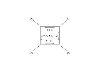
Figure 2: One-loop massless scalar triangle in momentum space

This box integral over Feynman parameters

$$\int\limits_{0}^{1}\int\limits_{0}^{1}\int\limits_{0}^{1}\int\limits_{0}^{1}\frac{\delta\left(\sum\limits_{i=1}^{4}\alpha_{i}-1\right)\prod\limits_{i=1}^{4}d\alpha_{i}}{[\alpha_{1}\alpha_{2}p_{1}^{2}+\alpha_{2}\alpha_{3}p_{2}^{2}+\alpha_{3}\alpha_{4}p_{3}^{2}+\alpha_{1}\alpha_{4}p_{4}^{2}+\alpha_{1}\alpha_{3}s+\alpha_{2}\alpha_{4}t]^{2}}$$ (24)

corresponds to all the indices 1 and $d=4.$

4.5 From the box to the triangle via Feynman parameters

In the paper [3] it has been shown that the box diagram and the triangle diagram are equivalent under the condition that all the indices of the propagators are 1 and the dimension of the spacetime is 4 exactly. In Appendix A we give a brief review of the trick used in [3] which suggests a combination of the Feynman formula and Mellin-Barnes integral representation. We reproduce it just to show that we may avoid extensive mixture of Feynman formula and Mellin-Barnes transformation and may work only in terms of MB transformation from the very beginning. In essence, we compare pure MB approach and the approach of Usyukina and Davydychev. We just would like to notice that the pure MB approach is necessary to elaborate the strategy in order to reduce the number of contour integrals what basically is equivalent to reduction of the rank of the corresponding series resulting from evaluation of the residues by Cauchy integral formula. Reduction of the rank of the resulting special functions means that some of the contours contribute with a finite number of residues that is highly unusual for the Barnes integrals because the Euler gamma functions produce infinite number of residues. Any Barnes integral may be represented in terms of special functions, no matter if the integrals over Feynman parameters contribute with a finite number of residues or with an infinite number of residues in the complex planes of the corresponding complex integrals.

In the next Subsection 4.6 of the present article we show that the MB representation of (24) is enough to reduce the number of independent arguments in the resulting hypergeometry, that is, to reduce the rank of the resulting hypergeometry and it is not necessary to use Feynman formula at an intermediate step. We map the Feynman formula (24) to the MB representation at the initial step, and then never go back, all the work is done by the analytical regularization of the divergent integrals over Feynman parameters in the integrand of the contour Mellin-Barnes integrals.

Also, we need to comment that the trick of [3] is not the unique way to transform the triangle ladder diagram to the box ladder diagram. The simplest way is to apply conformal transformation in an auxiliary position space which is dual to the momentum space [7, 8]

4.6 The five-fold MB box is the two-fold MB triangle

Our task is to reproduce the same result (A.1) directly from the integral (24) which is an integral over Feynman parameters. This will help us to elaborate a strategy how to reduce the number of contour integration in the MB representations of the integrals over Feynman parameters in a more general case of arbitrary spacetime dimension and arbitrary indices of the propagators. The strategy that is formulated in the next Section 5 is based on the experience we gain in this Section 4.6. Advantage of such an approach is that the calculation via MB works everywhere while the trick of Usyukina and Davydychev described in Appendix A works only for very special cases when the indices of the propagators and the dimension of spacetime are related. The integrals over Feynman parameters result in product of the Euler beta functions via the algorithm we have outlined in Subsection 4.3, however it may happen that an additional regularization of singularities is required in order to represent such integrals in terms of the Euler beta functions. Remarkably, when such singularities appear in the integration over the straight lines in the Barnes integrals, the number of the integration contours in the corresponding complex domains may be reduced.

We show in this section 4.6 how the multi-fold MB integrals may be reduced to the two-fold MB integrals. The multi-fold MB integrals we consider here are produced from the integrals over Feynman parameters like for example (24). The reason for such a reduction is in an efficient regularization of the divergent integrals over Feynman parameters. We observe that each integral over Feynman parameters regularized analytically produces infinite number of residues (as usual for the Euler beta function) but only one of them contributes in the limit of removing the analytical regularization. These residues are situated in certain complex planes which correspond to certain linear combinations of the MB integration variables. When the sum of the powers of the Feynman parameters after the MB transformation of denominators is a non-positive integer, a rearrangement of the MB integration variables in their complex planes is necessary. Below we explain how to establish which combination of MB variables contributes with a finite number of residues. The example considered in this Subsection 4.6 explains how to rearrange the variables in order to reduce maximally the number of the integration contours.

First of all, this is the five-fold MB transformation because of the six terms in the denominator

$$\int\limits_{0}^{1}\int\limits_{0}^{1}\int\limits_{0}^{1}\int\limits_{0}^{1}\frac{\delta\left(\sum\limits_{i=1}^{4}\alpha_{i}-1\right)\prod\limits_{i=1}^{4}d\alpha_{i}}{(\alpha_{1}\alpha_{2}p_{1}^{2}+\alpha_{2}\alpha_{3}p_{2}^{2}+\alpha_{3}\alpha_{4}p_{3}^{2}+\alpha_{1}\alpha_{4}p_{4}^{2}+\alpha_{1}\alpha_{3}s+\alpha_{2}\alpha_{4}t)^{2}}$$

$$=\int\limits_{-\delta_{1}-i\infty}^{-\delta_{1}+i\infty}~{}dz_{1}\int\limits_{-\delta_{2}-i\infty}^{-\delta_{2}+i\infty}~{}dz_{2}\int\limits_{-\delta_{3}-i\infty}^{-\delta_{3}+i\infty}~{}dz_{3}\int\limits_{-\delta_{4}-i\infty}^{-\delta_{4}+i\infty}~{}dz_{4}\int\limits_{-\delta_{5}-i\infty}^{-\delta_{5}+i\infty}~{}dz_{5}\Gamma(-z_{1})\Gamma(-z_{2})\Gamma(-z_{3})\Gamma(-z_{4})$$

$$\times\Gamma(-z_{5})\Gamma(2+z_{1}+z_{2}+z_{3}+z_{4}+z_{5})\int\limits_{0}^{1}\int\limits_{0}^{1}\int\limits_{0}^{1}\int\limits_{0}^{1}\frac{\delta\left(\sum\limits_{i=1}^{4}\alpha_{i}-1\right)\prod\limits_{i=1}^{4}d\alpha_{i}}{(\alpha_{1}\alpha_{2}p_{1}^{2})^{2}}$$

$$\times\left(\frac{\alpha_{2}\alpha_{3}p_{2}^{2}}{\alpha_{1}\alpha_{2}p_{1}^{2}}\right)^{z_{1}}\left(\frac{\alpha_{3}\alpha_{4}p_{3}^{2}}{\alpha_{1}\alpha_{2}p_{1}^{2}}\right)^{z_{2}}\left(\frac{\alpha_{1}\alpha_{4}p_{4}^{2}}{\alpha_{1}\alpha_{2}p_{1}^{2}}\right)^{z_{3}}\left(\frac{\alpha_{1}\alpha_{3}s}{\alpha_{1}\alpha_{2}p_{1}^{2}}\right)^{z_{4}}\left(\frac{\alpha_{2}\alpha_{4}t}{\alpha_{1}\alpha_{2}p_{1}^{2}}\right)^{z_{5}}$$

$$=\frac{1}{(p_{1}^{2})^{2}}\int\limits_{-\delta_{1}-i\infty}^{-\delta_{1}+i\infty}~{}dz_{1}\int\limits_{-\delta_{2}-i\infty}^{-\delta_{2}+i\infty}~{}dz_{2}\int\limits_{-\delta_{3}-i\infty}^{-\delta_{3}+i\infty}~{}dz_{3}\int\limits_{-\delta_{4}-i\infty}^{-\delta_{4}+i\infty}~{}dz_{4}\int\limits_{-\delta_{5}-i\infty}^{-\delta_{5}+i\infty}~{}dz_{5}\Gamma(-z_{1})\Gamma(-z_{2})$$

$$\times\Gamma(-z_{3})\Gamma(-z_{4})\Gamma(-z_{5})\Gamma(2+z_{1}+z_{2}+z_{3}+z_{4}+z_{5})\left(\frac{p_{2}^{2}}{p_{1}^{2}}\right)^{z_{1}}\left(\frac{p_{3}^{2}}{p_{1}^{2}}\right)^{z_{2}}\left(\frac{p_{4}^{2}}{p_{1}^{2}}\right)^{z_{3}}\left(\frac{s}{p_{1}^{2}}\right)^{z_{4}}$$

$$\left(\frac{t}{p_{1}^{2}}\right)^{z_{5}}\int\limits_{0}^{1}\int\limits_{0}^{1}\int\limits_{0}^{1}\int\limits_{0}^{1}\delta\left(\sum_{i=1}^{4}\alpha_{i}-1\right)~{}\alpha_{1}^{-2-z_{1}-z_{2}-z_{5}}\alpha_{2}^{-2-z_{2}-z_{3}-z_{4}}\alpha_{3}^{z_{1}+z_{2}+z_{4}}\alpha_{4}^{z_{2}+z_{3}+z_{5}}\prod_{i=1}^{4}d\alpha_{i}$$ (25)

The hierarchy of the contour positions in the multi-fold MB transformation considered in Section 2 suggests

$${\rm Re}~{}\lambda>0$$

$${\rm Re}~{}\lambda>\delta_{1}>0$$

$${\rm Re}~{}\lambda-\delta_{1}>\delta_{2}>0$$

$${\rm Re}~{}\lambda-\delta_{1}-\delta_{2}>\delta_{3}>0$$

$${\rm Re}~{}\lambda-\delta_{1}-\delta_{2}-\delta_{3}>\delta_{4}>0$$

$${\rm Re}~{}\lambda-\delta_{1}-\delta_{2}-\delta_{3}-\delta_{4}>\delta_{5}>0$$

We converted the integration over the simplex into the integration over the unit cube in the way established in Subsection 4.3. This is a universal step in order to take the integration over the Feynman parameters off. An intermediate analytical regularization may be necessary to generate certain ratios of the Euler gamma functions. In Subsection 4.1 we have not used any analytical intermediate regularization supposing that the indices belong to the domain of the convergence at both the limits, upper and lower. The result is a Barnes integral in the integrand of which there is a product of the gamma functions divided by another product of the gamma functions. In case when $\Gamma(-n+\varepsilon)$ in the denominator is generated, $\varepsilon$ is a complex parameter of the analytic regularization, the integration becomes simple because only a few residues contribute to the limit $\varepsilon\rightarrow 0$ in which we remove the intermediate analytical regularization. A similar situation may be discovered for the uniqueness case [28] however the $\Gamma(0)$ has appeared in the denominator by construction due to the uniqueness condition but not due to the integration over Feynman parameters as we obtain here. In the integral (4.6) that we consider in the present paper the structure of the MB integrands repeats the structure of the integrands used to prove the orthogonality of triangles in [28]. This fact suggests to rearrange variables of MB integration in order to make it explicit which combinations of the initial complex variables should be integrated out in the first few steps.

Suppose that we intent to convert the integral over the simplex in the last line of Eq. (4.6) into the integral over the unit cube by using Eq. (23) from Subsection 4.3. However, this integral over simplex is divergent for each of the powers of the Feynman variables which are given in this last line of (4.6). The natural question may be asked. Namely, can we make a change of variables in a divergent integral over a simplex with these given powers of Feynman variables? The real parts of these complex powers are fixed by the positions of the straight vertical lines in the integration contours of the complex domains of the MB integrals for the inverse transformation in (4.6). The powers of the Feynman parameters in the last line of (4.6) are integrated over five contours with another function of these powers from the integrand of the contour integral and this overall integral in five complex domains is convergent. In turn, the convergence of this overall integral over five complex contours means that the last line of (4.6) should be understood in a sense of distributions and a change of variables for the multiple integral over three Feynman parameters may be done. By changing the simplex to the unit cube we obtain

$$\int\limits_{0}^{1}\int\limits_{0}^{1}\int\limits_{0}^{1}\int\limits_{0}^{1}\delta\left(\sum_{i=1}^{4}\alpha_{i}-1\right)~{}\alpha_{1}^{-2-z_{1}-z_{2}-z_{5}}\alpha_{2}^{-2-z_{2}-z_{3}-z_{4}}\alpha_{3}^{z_{1}+z_{2}+z_{4}}\alpha_{4}^{z_{2}+z_{3}+z_{5}}\prod_{i=1}^{4}d\alpha_{i}$$

$$=\int\limits_{0}^{1}~{}d\alpha_{4}~{}\alpha_{4}^{z_{2}+z_{3}+z_{5}}(1-\alpha_{4})^{-2-z_{5}-z_{2}-z_{3}}\int\limits_{0}^{1}d\beta_{3}(1-\beta_{3})^{-3-z_{1}-2z_{2}-z_{3}-z_{4}-z_{5}}\beta_{3}^{z_{1}+z_{2}+z_{4}}$$

$$\times\int\limits_{0}^{1}d\gamma_{2}~{}(1-\gamma_{2})^{-2-z_{1}-z_{2}-z_{5}}\gamma_{2}^{-2-z_{2}-z_{3}-z_{4}}.$$ (26)

This means that in the formula (23) the powers of the Feynman variables are chosen to take these values

$$z = -2-z_{1}-z_{2}-z_{5}$$

$$u = -2-z_{2}-z_{3}-z_{4}$$

$$v = z_{1}+z_{2}+z_{4}$$

$$w = z_{2}+z_{3}+z_{5},$$

The powers of Feynman parameters were supposed to belong to the convergent domain in formula (23). However, in Eq. (26) we cannot suppose the same because the powers are not in the domain of convergence. As we have explained in the previous paragraph, we still may change the integration domain for the triple integral over Feynman parameters from the simplex to the unit cube because of the overall convergence of this five-fold MB integral (4.6). As the result, all these three integrals on the rhs of of (26) are divergent for the powers situated at the positions of the straight vertical lines in the expression (4.6). Because the initial integral over Feynman parameters (24) is convergent, the integral over a simplex may be separated in a product of three integrals even in this case when they are not convergent for such positions of the contours. The convergence of the overall integral suggests that we may shift the powers in these three integrals in such a way that each of them becomes convergent and equal to the Euler beta function. A similar idea has been used in [43, 44]. Then, under this auxiliary analytical regularization the three resulting Euler beta functions on the r.h.s. of (26) should be understood in the limit of the removing this auxiliary regularization [43, 44] as distributions which are integrated with the rest of the complex integrand over all the five contours. Then, the residues may be calculated according to the integral Cauchy formula. We show that only a finite number of residues survives in this limit of the removing regularization. This happens due to the singular behavior of these three unregularized integrals on the rhs of (26). It is singular because the powers of the Feynman variables belong to the straight vertical lines of the MB integration contours.

Now we recombine the complex integration variables, taking into account of course the simple structure (A.1) we “search” in order to prove it

$$\frac{1}{(p_{1}^{2})^{2}}\int\limits_{-\delta_{1}-i\infty}^{-\delta_{1}+i\infty}~{}dz_{1}\int\limits_{-\delta_{2}-i\infty}^{-\delta_{2}+i\infty}~{}dz_{2}\int\limits_{-\delta_{3}-i\infty}^{-\delta_{3}+i\infty}~{}dz_{3}\int\limits_{-\delta_{4}-i\infty}^{-\delta_{4}+i\infty}~{}dz_{4}\int\limits_{-\delta_{5}-i\infty}^{-\delta_{5}+i\infty}~{}dz_{5}\Gamma(-z_{1})\Gamma(-z_{2})\Gamma(-z_{3})$$

$$\times\Gamma(-z_{4})\Gamma(-z_{5})\Gamma(2+z_{1}+z_{2}+z_{3}+z_{4}+z_{5})\left(\frac{p_{2}^{2}}{p_{1}^{2}}\right)^{z_{1}}\left(\frac{p_{3}^{2}}{p_{1}^{2}}\right)^{z_{2}}\left(\frac{p_{4}^{2}}{p_{1}^{2}}\right)^{z_{3}}\left(\frac{s}{p_{1}^{2}}\right)^{z_{4}}$$

$$\left(\frac{t}{p_{1}^{2}}\right)^{z_{5}}\int\limits_{0}^{1}\int\limits_{0}^{1}\int\limits_{0}^{1}\int\limits_{0}^{1}\delta\left(\sum_{i=1}^{4}\alpha_{i}-1\right)~{}\alpha_{1}^{-2-z_{1}-z_{2}-z_{5}}\alpha_{2}^{-2-z_{2}-z_{3}-z_{4}}\alpha_{3}^{z_{1}+z_{2}+z_{4}}\alpha_{4}^{z_{2}+z_{3}+z_{5}}\prod_{i=1}^{4}d\alpha_{i}$$

$$=\frac{1}{(p_{1}^{2})^{2}}\int\limits_{-\delta_{1}-i\infty}^{-\delta_{1}+i\infty}~{}dz_{1}\int\limits_{-\delta_{2}-i\infty}^{-\delta_{2}+i\infty}~{}dz_{2}\int\limits_{-\delta_{3}-i\infty}^{-\delta_{3}+i\infty}~{}dz_{3}\int\limits_{-\delta_{4}-i\infty}^{-\delta_{4}+i\infty}~{}dz_{4}\int\limits_{-\delta_{5}-i\infty}^{-\delta_{5}+i\infty}~{}dz_{5}\Gamma(-z_{1})\Gamma(-z_{2})\Gamma(-z_{3})$$

$$\times\Gamma(-z_{4})\Gamma(-z_{5})\Gamma(2+z_{1}+z_{2}+z_{3}+z_{4}+z_{5})\left(\frac{p_{2}^{2}}{p_{1}^{2}}\right)^{z_{1}}\left(\frac{p_{3}^{2}}{p_{1}^{2}}\right)^{z_{2}}\left(\frac{p_{4}^{2}}{p_{1}^{2}}\right)^{z_{3}}\left(\frac{s}{p_{1}^{2}}\right)^{z_{4}}\left(\frac{t}{p_{1}^{2}}\right)^{z_{5}}$$

$$\int\limits_{0}^{1}~{}d\alpha_{4}~{}\alpha_{4}^{z_{2}+z_{3}+z_{5}}(1-\alpha_{4})^{-2-z_{5}-z_{2}-z_{3}}\int\limits_{0}^{1}d\beta_{3}(1-\beta_{3})^{-3-z_{1}-2z_{2}-z_{3}-z_{4}-z_{5}}\beta_{3}^{z_{1}+z_{2}+z_{4}}$$

$$\int\limits_{0}^{1}d\gamma_{2}~{}(1-\gamma_{2})^{-2-z_{1}-z_{2}-z_{5}}\gamma_{2}^{-2-z_{2}-z_{3}-z_{4}}$$

$$=\frac{1}{st}\int\limits_{-\delta_{1}-i\infty}^{-\delta_{1}+i\infty}~{}dz_{1}\int\limits_{-\delta_{2}-i\infty}^{-\delta_{2}+i\infty}~{}dz_{2}\int\limits_{-\delta_{3}-i\infty}^{-\delta_{3}+i\infty}~{}dz_{3}\int\limits_{-\delta_{4}-i\infty}^{-\delta_{4}+i\infty}~{}dz_{4}\int\limits_{-\delta_{5}-i\infty}^{-\delta_{5}+i\infty}~{}dz_{5}\Gamma(-z_{1})\Gamma(-z_{2})$$

$$\times\Gamma(-z_{3})\Gamma(-z_{4})\Gamma(-z_{5})\Gamma(2+z_{1}+z_{2}+z_{3}+z_{4}+z_{5})\left(\frac{p_{2}^{2}p_{4}^{2}}{st}\right)^{z_{1}}\left(\frac{p_{3}^{2}p_{1}^{2}}{st}\right)^{z_{2}}$$

$$s^{z_{1}+z_{2}+z_{4}+1}t^{z_{1}+z_{2}+z_{5}+1}\left(p_{4}^{2}\right)^{-z_{1}+z_{3}}\left(p_{1}^{2}\right)^{-z_{1}-2z_{2}-z_{3}-z_{4}-z_{5}-2}$$

$$\int\limits_{0}^{1}~{}d\alpha_{4}~{}\alpha_{4}^{z_{2}+z_{3}+z_{5}}(1-\alpha_{4})^{-2-z_{5}-z_{2}-z_{3}}\int\limits_{0}^{1}d\beta_{3}(1-\beta_{3})^{-3-z_{1}-2z_{2}-z_{3}-z_{4}-z_{5}}\beta_{3}^{z_{1}+z_{2}+z_{4}}$$

$$\int\limits_{0}^{1}d\gamma_{2}~{}(1-\gamma_{2})^{-2-z_{1}-z_{2}-z_{5}}\gamma_{2}^{-2-z_{2}-z_{3}-z_{4}}$$

$$=\frac{1}{st}\int\limits_{-\delta_{1}-i\infty}^{-\delta_{1}+i\infty}~{}dz_{1}\Gamma(-z_{1})\int\limits_{-\delta_{2}-i\infty}^{-\delta_{2}+i\infty}~{}dz_{2}~{}\Gamma(-z_{2})\int\limits_{1-\delta_{2}-\delta_{2}-\delta_{5}-i\infty}^{1-\delta_{1}-\delta_{2}-\delta_{5}+i\infty}~{}du~{}\Gamma(1+z_{1}+z_{2}-u)$$

$$\int\limits_{\delta_{1}-\delta_{3}-i\infty}^{\delta_{1}-\delta_{3}+i\infty}~{}dv~{}\Gamma(-v-z_{1})\int\limits_{1-\delta_{1}-\delta_{2}-\delta_{4}-i\infty}^{1-\delta_{1}-\delta_{2}-\delta_{4}+i\infty}~{}dw~{}\Gamma(1+z_{1}+z_{2}-w)\Gamma(u+w+v-z_{2})$$

$$\left(\frac{p_{2}^{2}p_{4}^{2}}{st}\right)^{z_{1}}\left(\frac{p_{3}^{2}p_{1}^{2}}{st}\right)^{z_{2}}s^{w}t^{u}\left(p_{4}^{2}\right)^{v}\left(p_{1}^{2}\right)^{-v-w-u}$$

$$\int\limits_{0}^{1}~{}d\alpha_{4}~{}\alpha_{4}^{v+u-1}(1-\alpha_{4})^{-1-u-v}\int\limits_{0}^{1}d\beta_{3}(1-\beta_{3})^{-v-w-u-1}\beta_{3}^{w-1}\int\limits_{0}^{1}d\gamma_{2}~{}(1-\gamma_{2})^{-u-1}\gamma_{2}^{-1-v-w}$$ (27)

Here we have introduced new complex variables

$$w = z_{1}+z_{2}+z_{4}+1$$

$$u = z_{1}+z_{2}+z_{5}+1$$ (28)

$$v = -z_{1}+z_{3}$$

As we have mentioned in the previous paragraphs of this Subsection 4.6, exactly these combinations of the initial MB integration variables may be integrated out by the Cauchy integral formula with a finite number of residues. In this particular case each of them is integrated out with one residue only. The rest of the infinite number of residues does snot contribute for any of these three variables $u,v,w.$

In order to analyze convergence of the integrals over the Feynman parameters in the last line of (4.6) at the integration limits at the points 1 and 0, it is necessary to take into account the values of the real parts of these new variables $u,w,z$ given by the positions of the straight vertical lines of the contours of the initial MB integration variables. The integral over $\alpha_{4}$ in the last line of (4.6) is not convergent at its upper limit for the values of $u$ and $v$ on the straight vertical lines of the $u$ and $v$ integration contours. However, we know that the overall five-fold integral (4.6) (this is the same structure (4.6) but in terms of new variables) is finite because the original integral (24) over the Feynman parameters is finite. This means that

$$\int\limits_{0}^{1}~{}d\alpha_{4}~{}\alpha_{4}^{v+u-1}(1-\alpha_{4})^{-1-u-v}$$ (29)

should be understood in a sense of distributions over the new complex variables $u$ and $v,$ that is, the integral (4.6) may be concisely written as

$$\frac{1}{st}\int\limits_{1-\delta_{1}-\delta_{2}-\delta_{5}-i\infty}^{1-\delta_{1}-\delta_{2}-\delta_{5}+i\infty}~{}du\int\limits_{\delta_{1}-\delta_{3}-i\infty}^{\delta_{1}-\delta_{3}+i\infty}~{}dv~{}f_{1}(u,v)~{}\int\limits_{0}^{1}~{}d\alpha_{4}~{}\alpha_{4}^{v+u-1}(1-\alpha_{4})^{-1-u-v},$$ (30)

$f_{1}(u,v)$ here stands for the rest of the integrand in (4.6). The five-fold integral (4.6) is not singular, it takes a finite value. This means that (29) may be replaced in (30) with a limit which regularizes (29), that is,

$$\lim_{\varepsilon_{1}\rightarrow 0}\int\limits_{1-\delta_{1}-\delta_{2}-\delta_{5}-i\infty}^{1-\delta_{1}-\delta_{2}-\delta_{5}+i\infty}~{}du\int\limits_{\delta_{1}-\delta_{3}-i\infty}^{\delta_{1}-\delta_{3}+i\infty}~{}dv~{}f_{1}(u,v)~{}\int\limits_{0}^{1}~{}d\alpha_{4}~{}\alpha_{4}^{v+u-1}(1-\alpha_{4})^{-1-u-v+\varepsilon_{1}}$$

$$=\lim_{\varepsilon_{1}\rightarrow 0}\int\limits_{1-\delta_{1}-\delta_{2}-\delta_{5}-i\infty}^{1-\delta_{1}-\delta_{2}-\delta_{5}+i\infty}~{}du\int\limits_{\delta_{1}-\delta_{3}-i\infty}^{\delta_{1}-\delta_{3}+i\infty}~{}dv~{}f_{1}(u,v)~{}\frac{\Gamma(v+u)\Gamma(-u-v+\varepsilon_{1})}{\Gamma(\varepsilon_{1})}$$

$$=\int\limits_{\delta_{1}-\delta_{3}-i\infty}^{\delta_{1}-\delta_{3}+i\infty}~{}dv~{}f_{1}(0,v),$$

where we suppose that we have started with ${\rm Re~{}~{}}\varepsilon_{1}>2$. This trick has been applied in [44, 43]. Apparently, the pole $u=\varepsilon_{1}-v$ in the complex $u$ plane contributes because it is on the right hand side of the straight vertical line in the complex plane of the variable $u$ when ${\rm Re~{}~{}}\varepsilon_{1}>2,$

$$\mathop{{\rm Res}}\limits_{u=\varepsilon_{1}-v}\frac{\Gamma(v+u)\Gamma(-u-v+\varepsilon_{1})}{\Gamma(\varepsilon_{1})}=\mathop{{\rm Res}}\limits_{u=\varepsilon_{1}-v}\frac{\Gamma(v+u)\Gamma(1-u-v+\varepsilon_{1})}{\Gamma(\varepsilon_{1})(-u-v+\varepsilon_{1})}=-\frac{\Gamma(\varepsilon_{1})}{\Gamma(\varepsilon_{1})}=-1.$$

This is the only residue in the complex $u$ plane that contributes, other residues disappear in the limit of removing the regularization. However, this residue before taking the limit was on the right hand side, it was a right residue, it contributes with the negative sign due to the clockwise orientation of the corresponding contour integral. The contributions of other residues produced by $\Gamma(-u-v+\varepsilon_{1})$ in the complex $u$ plane will vanish in this limit of the removing the regularization because $\Gamma(\varepsilon_{1})$ will not appear in their numerator, there is nothing to compensate $\Gamma(\varepsilon_{1})$ in the denominator as it happened for the first residue at $u=\varepsilon_{1}-v.$ Alternatively, if we close the MB integration contour to the left complex infinity for the variable $u,$ the situation will be the same. Only the first pole at $u=-v$ produced by $\Gamma(u+v)$ contributes in this case. The contributions of other residues produced by $\Gamma(u+v)$ vanish in the limit of removing the regularization $\varepsilon_{1}\rightarrow 0.$

Thus, the five-fold MB integral (4.6) may be replaced with a four-fold MB integral

$$\frac{1}{st}\int\limits_{-\delta_{1}-i\infty}^{-\delta_{1}+i\infty}~{}dz_{1}\Gamma(-z_{1})\int\limits_{-\delta_{2}-i\infty}^{-\delta_{2}+i\infty}~{}dz_{2}~{}\Gamma(-z_{2})\int\limits_{1-\delta_{1}-\delta_{2}-\delta_{5}-i\infty}^{1-\delta_{1}-\delta_{2}-\delta_{5}+i\infty}~{}du~{}\Gamma(1+z_{1}+z_{2}-u)$$

$$\int\limits_{\delta_{1}-\delta_{3}-i\infty}^{\delta_{1}-\delta_{3}+i\infty}~{}dv~{}\Gamma(-v-z_{1})\int\limits_{1-\delta_{1}-\delta_{2}-\delta_{4}-i\infty}^{1-\delta_{1}-\delta_{2}-\delta_{4}+i\infty}~{}dw~{}\Gamma(1+z_{1}+z_{2}-w)\Gamma(u+w+v-z_{2})$$

$$\left(\frac{p_{2}^{2}p_{4}^{2}}{st}\right)^{z_{1}}\left(\frac{p_{3}^{2}p_{1}^{2}}{st}\right)^{z_{2}}s^{w}t^{u}\left(p_{4}^{2}\right)^{v}\left(p_{1}^{2}\right)^{-v-w-u}$$

$$\int\limits_{0}^{1}~{}d\alpha_{4}~{}\alpha_{4}^{v+u-1}(1-\alpha_{4})^{-1-u-v}\int\limits_{0}^{1}d\beta_{3}(1-\beta_{3})^{-v-w-u-1}\beta_{3}^{w-1}\int\limits_{0}^{1}d\gamma_{2}~{}(1-\gamma_{2})^{-u-1}\gamma_{2}^{-1-v-w}$$

$$=\lim_{\varepsilon_{1}\rightarrow 0}\frac{1}{st}\int\limits_{-\delta_{1}-i\infty}^{-\delta_{1}+i\infty}~{}dz_{1}\Gamma(-z_{1})\int\limits_{-\delta_{2}-i\infty}^{-\delta_{2}+i\infty}~{}dz_{2}~{}\Gamma(-z_{2})\int\limits_{1-\delta_{1}-\delta_{2}-\delta_{5}-i\infty}^{1-\delta_{1}-\delta_{2}-\delta_{5}+i\infty}~{}du~{}\Gamma(1+z_{1}+z_{2}-u)$$

$$\int\limits_{\delta_{1}-\delta_{3}-i\infty}^{\delta_{1}-\delta_{3}+i\infty}~{}dv~{}\Gamma(-v-z_{1})\int\limits_{1-\delta_{1}-\delta_{2}-\delta_{4}-i\infty}^{1-\delta_{1}-\delta_{2}-\delta_{4}+i\infty}~{}dw~{}\Gamma(1+z_{1}+z_{2}-w)\Gamma(u+w+v-z_{2})$$

$$\times\frac{\Gamma(v+u)\Gamma(-u-v+\varepsilon_{1})}{\Gamma(\varepsilon_{1})}\left(\frac{p_{2}^{2}p_{4}^{2}}{st}\right)^{z_{1}}\left(\frac{p_{3}^{2}p_{1}^{2}}{st}\right)^{z_{2}}s^{w}t^{u}\left(p_{4}^{2}\right)^{v}\left(p_{1}^{2}\right)^{-v-w-u}$$

$$\times\int\limits_{0}^{1}d\beta_{3}(1-\beta_{3})^{-v-w-u-1}\beta_{3}^{w-1}\int\limits_{0}^{1}d\gamma_{2}~{}(1-\gamma_{2})^{-u-1}\gamma_{2}^{-1-v-w}$$

$$=\frac{1}{st}\int\limits_{-\delta_{1}-i\infty}^{-\delta_{1}+i\infty}~{}dz_{1}~{}\Gamma(-z_{1})\int\limits_{-\delta_{2}-i\infty}^{-\delta_{2}+i\infty}~{}dz_{2}~{}\Gamma(-z_{2})\int\limits_{\delta_{1}-\delta_{3}-i\infty}^{\delta_{1}-\delta_{3}+i\infty}~{}dv\Gamma(-v-z_{1})\Gamma(1+z_{1}+z_{2}+v)$$

$$\int\limits_{1-\delta_{1}-\delta_{2}-\delta_{4}-i\infty}^{1-\delta_{1}-\delta_{2}-\delta_{4}+i\infty}~{}dw~{}\Gamma(1+z_{1}+z_{2}-w)\Gamma(w-z_{2})\left(\frac{p_{2}^{2}p_{4}^{2}}{st}\right)^{z_{1}}\left(\frac{p_{3}^{2}p_{1}^{2}}{st}\right)^{z_{2}}s^{w}t^{-v}$$

$$\times\left(p_{4}^{2}\right)^{v}\left(p_{1}^{2}\right)^{-w}\int\limits_{0}^{1}d\beta_{3}(1-\beta_{3})^{-w-1}\beta_{3}^{w-1}\int\limits_{0}^{1}d\gamma_{2}~{}(1-\gamma_{2})^{v-1}\gamma_{2}^{-1-w-v}$$ (31)

The integral over $\beta_{3}$ is not convergent at the upper limit for ${\rm Re~{}~{}}w$ defined by Eq. (4.6) but at the lower limit is convergent. However, we know that the overall five-fold integral (4.6) is finite because the original integral (24) over the Feynman parameters is finite. This means that

$$\int\limits_{0}^{1}~{}d\beta_{3}~{}\beta_{3}^{w-1}(1-\beta_{3})^{-1-w}$$ (32)

should be understood in a sense of a distribution over the new complex variable $w$ that is, the integral (4.6) may be concisely written as

$$\int\limits_{1-\delta_{1}-\delta_{2}-\delta_{4}-i\infty}^{1-\delta_{1}-\delta_{2}-\delta_{4}+i\infty}~{}dw~{}f_{2}(w)\int\limits_{0}^{1}d\beta_{3}(1-\beta_{3})^{-w-1}\beta_{3}^{w-1}$$ (33)

$f_{2}(w)$ here stands for the rest of the integrand in (4.6). The four-fold integral (4.6) is not singular, it takes a finite value. This means that (32) may be replaced in (33) with a limit which regularizes it, that is,

$$\lim_{\varepsilon_{2}\rightarrow 0}\int\limits_{1-\delta_{1}-\delta_{2}-\delta_{4}-i\infty}^{1-\delta_{1}-\delta_{2}-\delta_{4}+i\infty}~{}dw~{}f_{2}(w)\int\limits_{0}^{1}d\beta_{3}(1-\beta_{3})^{-w-1}\beta_{3}^{w-1+\varepsilon_{2}}$$

$$=\lim_{\varepsilon_{2}\rightarrow 0}\int\limits_{1-\delta_{1}-\delta_{2}-\delta_{4}-i\infty}^{1-\delta_{1}-\delta_{2}-\delta_{4}+i\infty}~{}dw~{}f_{2}(w)\frac{\Gamma(w)\Gamma(-w+\varepsilon_{2})}{\Gamma(\varepsilon_{2})}=f_{2}(0),$$

where we suppose that we have started with ${\rm Re~{}~{}}\varepsilon_{2}>2.$ Apparently, the pole $w=\varepsilon_{2}$ in the complex $w$ plane contributes because it is on the right hand side of the straight vertical line in the complex plane of the variable $w$ when ${\rm Re~{}~{}}\varepsilon_{2}>2,$

$$\mathop{{\rm Res}}\limits_{w=\varepsilon_{2}}\frac{\Gamma(w)\Gamma(-w+\varepsilon_{2})}{\Gamma(\varepsilon_{2})}=\mathop{{\rm Res}}\limits_{w=\varepsilon_{2}}\frac{\Gamma(w)\Gamma(1-w+\varepsilon_{2})}{\Gamma(\varepsilon_{2})(-w+\varepsilon_{2})}=-\frac{\Gamma(\varepsilon_{2})}{\Gamma(\varepsilon_{2})}=-1.$$

This is the only residue in the complex $w$ plane that contributes, other residues disappear then in the limit of removing the regularization. The contributions of other residues produced by $\Gamma(-w+\varepsilon_{2})$ in the complex $w$ plane will vanish in this limit of the removing the regularization because $\Gamma(\varepsilon_{2})$ will not appear in their numerator, there is nothing to compensate $\Gamma(\varepsilon_{2})$ in the denominator in comparison as it happened for the first residue at $w=\varepsilon_{2}.$ However, this residue before taking the limit was on the right hand side of the straight line of the integration contour in the complex plane $w,$ it was a ”right” residue, it contributes with the negative sign due to the clockwise orientation of the corresponding contour integral. Alternatively, if we close the MB integration contour to the left complex infinity for the variable $w,$ the situation will be the same. Only the first pole at $w=0$ produced by $\Gamma(w)$ contributes in this case. The contributions of other residues produced by $\Gamma(w)$ vanish in the limit of removing the regularization $\varepsilon_{2}\rightarrow 0.$

Thus, the four-fold MB integral (4.6) integral may be replaced with three-fold MB integral

$$\frac{1}{st}\int\limits_{-\delta_{1}-i\infty}^{-\delta_{1}+i\infty}~{}dz_{1}~{}\Gamma(-z_{1})\int\limits_{-\delta_{2}-i\infty}^{-\delta_{2}+i\infty}~{}dz_{2}~{}\Gamma(-z_{2})\int\limits_{\delta_{1}-\delta_{3}-i\infty}^{\delta_{1}-\delta_{3}+i\infty}~{}dv\Gamma(-v-z_{1})$$

$$\Gamma(1+z_{1}+z_{2}+v)\int\limits_{1-\delta_{1}-\delta_{2}-\delta_{4}-i\infty}^{1-\delta_{1}-\delta_{2}-\delta_{4}+i\infty}~{}dw~{}\Gamma(1+z_{1}+z_{2}-w)\Gamma(w-z_{2})\left(\frac{p_{2}^{2}p_{4}^{2}}{st}\right)^{z_{1}}\left(\frac{p_{3}^{2}p_{1}^{2}}{st}\right)^{z_{2}}$$

$$s^{w}t^{-v}\left(p_{4}^{2}\right)^{v}\left(p_{1}^{2}\right)^{-w}\int\limits_{0}^{1}d\beta_{3}(1-\beta_{3})^{-w-1}\beta_{3}^{w-1}\int\limits_{0}^{1}d\gamma_{2}~{}(1-\gamma_{2})^{v-1}\gamma_{2}^{-1-w-v}$$

$$=\lim_{\varepsilon_{2}\rightarrow 0}\frac{1}{st}\int\limits_{-\delta_{1}-i\infty}^{-\delta_{1}+i\infty}~{}dz_{1}~{}\Gamma(-z_{1})\int\limits_{-\delta_{2}-i\infty}^{-\delta_{2}+i\infty}~{}dz_{2}~{}\Gamma(-z_{2})\int\limits_{\delta_{1}-\delta_{3}-i\infty}^{\delta_{1}-\delta_{3}+i\infty}~{}dv\Gamma(-v-z_{1})$$

$$\times\Gamma(1+z_{1}+z_{2}+v)\int\limits_{1-\delta_{1}-\delta_{2}-\delta_{4}-i\infty}^{1-\delta_{1}-\delta_{2}-\delta_{4}+i\infty}~{}dw~{}\Gamma(1+z_{1}+z_{2}-w)\Gamma(w-z_{2})$$

$$\left(\frac{p_{2}^{2}p_{4}^{2}}{st}\right)^{z_{1}}\left(\frac{p_{3}^{2}p_{1}^{2}}{st}\right)^{z_{2}}s^{w}t^{-v}\left(p_{4}^{2}\right)^{v}\left(p_{1}^{2}\right)^{-w}\frac{\Gamma(w)\Gamma(-w+\varepsilon_{2})}{\Gamma(\varepsilon_{2})}\int\limits_{0}^{1}d\gamma_{2}~{}(1-\gamma_{2})^{v-1}\gamma_{2}^{-1-v-w}$$

$$=\frac{1}{st}\int\limits_{-\delta_{1}-i\infty}^{-\delta_{1}+i\infty}~{}dz_{1}~{}\Gamma(-z_{1})\int\limits_{-\delta_{2}-i\infty}^{-\delta_{2}+i\infty}~{}dz_{2}~{}\Gamma(-z_{2})$$

$$\int\limits_{\delta_{1}-\delta_{3}-i\infty}^{\delta_{1}-\delta_{3}+i\infty}~{}dv\Gamma(-v-z_{1})\Gamma(1+z_{1}+z_{2}+v)\Gamma(1+z_{1}+z_{2})\Gamma(-z_{2})$$

$$\left(\frac{p_{2}^{2}p_{4}^{2}}{st}\right)^{z_{1}}\left(\frac{p_{3}^{2}p_{1}^{2}}{st}\right)^{z_{2}}t^{-v}\left(p_{4}^{2}\right)^{v}\int\limits_{0}^{1}d\gamma_{2}~{}(1-\gamma_{2})^{v-1}\gamma_{2}^{-1-v}$$ (34)

The integral over $\gamma_{2}$ is not convergent at the upper limit for ${\rm Re~{}~{}}v$ defined in Eq. (4.6), but at the lower limit is convergent because the value of $v$ is situated on the straight line with the fixed real part $\delta_{1}-\delta_{3}.$ However, we know that the overall five-fold integral (4.6) is finite because the original integral (24) over the Feynman parameters is finite. This means that the integral

$$\int_{0}^{1}~{}d\gamma_{2}~{}\gamma_{2}^{v-1}(1-\gamma_{2})^{-1-v}$$ (35)

should be understood in a sense of a distribution over the new complex variables $v$ that is, the integral (4.6) may be concisely written as

$$\int\limits_{\delta_{1}-\delta_{3}-i\infty}^{\delta_{1}-\delta_{3}+i\infty}~{}dvf_{3}(v)\int\limits_{0}^{1}~{}d\gamma_{2}~{}\gamma_{2}^{v-1}(1-\gamma_{2})^{-1-v}$$ (36)

$f_{3}(v)$ here stands for the rest of the integrand in (4.6). The three-fold integral (4.6) is not singular, it takes a finite value. This means that (35) may be replaced in (36) with a limit which regularizes (35), that is,

$$\int\limits_{\delta_{1}-\delta_{3}-i\infty}^{\delta_{1}-\delta_{3}+i\infty}~{}dvf_{3}(v)\int\limits_{0}^{1}~{}d\gamma_{2}~{}\gamma_{2}^{v-1}(1-\gamma_{2})^{-1-v}$$

$$=\lim_{\varepsilon_{3}\rightarrow 0}\int\limits_{\delta_{1}-\delta_{3}-i\infty}^{\delta_{1}-\delta_{3}+i\infty}~{}dvf_{3}(v)\int\limits_{0}^{1}~{}d\gamma_{2}~{}\gamma_{2}^{v-1}(1-\gamma_{2})^{-1-v+\varepsilon_{3}}$$

$$=\lim_{\varepsilon_{2}\rightarrow 0}\int\limits_{\delta_{1}-\delta_{3}-i\infty}^{\delta_{1}-\delta_{3}+i\infty}~{}dvf_{3}(v)\frac{\Gamma(v)\Gamma(-v+\varepsilon_{3})}{\Gamma(\varepsilon_{3})}=f_{3}(0).$$

where we suppose that we have started with ${\rm Re~{}~{}}\varepsilon_{3}>1.$ Apparently, the pole $v=\varepsilon_{3}$ in the complex $v$ plane contributes because it is on the right hand side of the straight vertical line in the complex plane of the variable $v$ when ${\rm Re~{}~{}}\varepsilon_{3}>1,$

$$\mathop{{\rm Res}}\limits_{v=\varepsilon_{3}}\frac{\Gamma(v)\Gamma(-v+\varepsilon_{3})}{\Gamma(\varepsilon_{3})}=\mathop{{\rm Res}}\limits_{v=\varepsilon_{3}}\frac{\Gamma(v)\Gamma(1-v+\varepsilon_{3})}{\Gamma(\varepsilon_{3})(-v+\varepsilon_{3})}=-\frac{\Gamma(\varepsilon_{3})}{\Gamma(\varepsilon_{3})}=-1.$$

This is the only residue in the complex $v$ plane that contributes, other residues disappear in the limit of removing the regularization. However, this residue before taking the limit was on the right hand side of the straight line of the integration contour in the complex plane $v,$ it was a ”right” residue, it contributes with the negative sign due to the clockwise orientation of the corresponding contour integral. Other residues in the complex plane of the variable $v$ contribute with $\Gamma(\varepsilon_{3})$ in the denominator and these contributions disappear when we take the limit $\varepsilon_{3}\rightarrow 0.$ They are produced by $\Gamma(-v+\varepsilon_{3})$ in the complex $v$ plane and will vanish in this limit of the removing the regularization because $\Gamma(\varepsilon_{3})$ will not appear in their numerator, there is nothing to compensate $\Gamma(\varepsilon_{3})$ in the denominator in comparison as it happened for the first residue at $v=\varepsilon_{3}.$ Alternatively, if we close the MB integration contour to the left complex infinity for the variable $v,$ the situation will be the same. Only the first pole at $v=0$ produced by $\Gamma(v)$ contributes in this case. The contributions of other residues produced by $\Gamma(v)$ vanish in the limit of removing the regularization $\varepsilon_{3}\rightarrow 0.$

5 Discussion

In quantum field theory, any Feynman diagram in any dimension can be expressed using Barnes integrals, whose integrands are ratios of Euler gamma functions. In massless theories, the structure of these integrands is somewhat simplified because there are no dimensional parameters like scales or masses. However, even in these theories, the number of Mellin-Barnes (MB) integration contours increases as the number of loops and external legs grows. In this paper we considered a case when a number of contours is efficiently reduced from the five-fold MB to the two-fold MB integration. This example of a simple massless box diagram known already for many years helps us to elaborate a general strategy which may be used for many Feynman diagrams, with masses or massless. Our observation highlights that certain integrals over Feynman parameters become singular after applying the MB transformation to the original integrals over Feynman parameters. These singular integrals must be treated as distributions in the remaining MB integrands. Analytical regularization is admitted here because the overall integral remains convergent. Upon applying analytical regularization, these distributions transform into Euler beta functions. The contributions from these beta functions reduce to a finite number of residues after the analytical regularization is removed. These residues correspond to specific new complex variables, which are linear combinations of the initial complex integration variables from the MB transformations. These linear combinations arise from the powers of the Feynman parameters in the singular integrals and can serve as new variables for the MB transformations. The finite set of residues in the planes of these new variables is straightforward to evaluate, leaving us with Barnes integrals where the number of contour integrations is reduced. This reduction corresponds to the number of singular integrals over Feynman parameters after the MB transformation applied to the denominator of the original integral over them.

The strategy for an arbitrary diagram is a quite straightforward generalization of the idea described in the previous paragraph. We take a Feynman diagram, apply the Feynman formula, transform the denominator in the integrand over the Feynman parameters to the Mellin-Barnes integral, transform the integral over $n$-simplex to the integral over the unit volume (this is the unit $(n-1)$-cube where $n$ is the number of Feynman parameters) and look which of the integrals over the Feynman parameters are singular. These singular integrals should be regularized by the analytical regularization. The regularized integrals result in the Euler beta functions which may be re-written as ratios of the Euler gamma functions. If in the denominator the gamma function of non-positive integer appears, the corresponding contour integral contributes with a finite number of residues. The true variables of these contour integrations coincide with powers of the singular integrals over the Feynman parameters, which are certain linear combinations of the initial MB integration variables. The initial arguments of the MB transformations may be re-grouped according to these linear combinations after taking the contour integrals over these linear combinations off by evaluation a finite number of residues. The rank of the special function of the re-grouped arguments which appears after taking all the MB integrations off, is reduced because the number of the MB integration contours is reduced.

The analytical regularization may be done only when the singular integrals are parts of the MB integrands and the overall MB integral is convergent. This is the case usually because it corresponds to a convergent overall integral over the Feynman parameters. Only in such a case the singular integrals over the Feynman parameters may be understood in a sense of distributions in the MB integrands and may be regularized analytically. For example, the left hand side of (10) cannot be analytically regularized if the integral is divergent, this would produce wrong results if done. At the same time, the inverse formula (5) is valid for any $\lambda$ even for a negative integer. This means that the integration domains of the left hand sides of (3) and (10) should be modified for $\lambda$ negative by contour deformations established in Refs. [45, 36, 46]. In turn, the modification of the left hand side of (10) would mean the modification of the Feynman formula (15) to another formula which will be valid after such a deformation of (10) to arbitrary indices $\nu_{i}$ and dimension $d.$ As we have seen in Subsection 4.1, the Feynman formula (16) for the case of the triangle diagram is valid for a wide domain of $\nu_{i}$ and $d$ determined by the requirement of convergence of the integrals in (16). It is possible based on the technique developed in [45, 36, 46] to find how the integral (16) should be modified in order to apply it for arbitrary indices and an arbitrary dimension. However, for the four-point box diagram, the divergent integrals over Feynman parameters appear in the MB integrand even for the convergent overall integral (24) when all the indices of the propagators are 1 and the dimension $d=4$. A modified Feynman formula would guarantee the convergence of these integrals in which the integration over the interval from 0 to 1 would be replaced with the integration over Pochhammer contour or over Hankel contour [45, 36, 46]. The analytical regularization in the MB integrands is not necessary if such a modified Feynman formula is used.

Acknowledgments

M.D. is supported by the fellowship of “Ayudante de investigacion de pregrado y postgrado 2021” of VRIP UBB. He is grateful to Andrei Davydychev and Cristian Villavicencio for careful reading of his thesis and for warm and constructive evaluation of his results during the thesis defence. I.G. would like to thank CEFITEV-UV for partial support. The work of I.K. was supported in part by Fondecyt (Chile) Grants Nos. 1040368, 1050512 and 1121030, by DIUBB (Chile) Grant Nos. 125009, GI 153209/C and GI 152606/VC. E.A.N.C. work was partially supported by DIDULS, Universidad de La Serena.

Appendix A The original way from the Triangle to the Box

We reproduce here the trick of Usyukina and Davydychev [3] that they used to relate the three-point and the four-point Green functions with only one purpose: to compare it with pure MB approach which we proposed in the present paper.

The integral (24) may be developed

$$\int\limits_{0}^{1}\int\limits_{0}^{1}\int\limits_{0}^{1}\int\limits_{0}^{1}d\alpha_{1}d\alpha_{2}d\alpha_{3}d\alpha_{4}\frac{\delta\left(\alpha_{1}+\alpha_{2}+\alpha_{3}+\alpha_{4}-1\right)}{\left[\alpha_{1}\left(\alpha_{2}p_{1}^{2}+\alpha_{3}s\right)+\alpha_{4}\left(\alpha_{3}p_{3}^{2}+\alpha_{2}t\right)+\alpha_{1}\alpha_{4}p_{4}^{2}+\alpha_{2}\alpha_{3}p_{2}^{2}\right]^{2}}$$

$$=\int\limits_{0}^{1}d\alpha_{4}\int\limits_{0}^{1-\alpha_{4}}d\alpha_{3}\int\limits_{0}^{1-\alpha_{4}-\alpha_{3}}d\alpha_{2}\int\limits_{0}^{1-\alpha_{4}-\alpha_{3}-\alpha_{2}}d\alpha_{1}\;\frac{\delta\left(\alpha_{1}+\alpha_{2}+\alpha_{3}+\alpha_{4}-1\right)}{\left[\alpha_{1}X+\alpha_{4}Y+\alpha_{1}\alpha_{4}p_{4}^{2}+\alpha_{2}\alpha_{3}p_{2}^{2}\right]^{2}},$$

where we have introduced the notation for $X$ and $Y$

$$X=\alpha_{2}p_{1}^{2}+\alpha_{3}s,~{}~{}~{}Y=\alpha_{3}p_{3}^{2}+\alpha_{2}t.$$

After removing the integral over $\alpha_{1}$ and changing then the integration variables $\alpha_{2}$ and $\alpha_{3}$ as

$$\alpha_{2}=(1-\alpha_{4})\beta_{2},~{}~{}~{}~{}\alpha_{3}=(1-\alpha_{4})\beta_{3},$$

we obtain

$$\int\limits_{0}^{1}d\alpha_{4}\int\limits_{0}^{1-\alpha_{4}}d\alpha_{3}\int\limits_{0}^{1-\alpha_{4}-\alpha_{3}}d\alpha_{2}\frac{1}{\left[(1-\alpha_{4}-\alpha_{3}-\alpha_{2})X+\alpha_{4}Y+(1-\alpha_{4}-\alpha_{3}-\alpha_{2})\alpha_{4}p_{4}^{2}+\alpha_{2}\alpha_{3}p_{2}^{2}\right]^{2}}$$

$$=\int\limits_{0}^{1}d\alpha_{4}\int\limits_{0}^{1}d\beta_{3}\int\limits_{0}^{1-\beta_{3}}d\beta_{2}\frac{\left(1-\alpha_{4}\right)^{2}}{\left[\left(1-\alpha_{4}\right)^{2}\left((1-\beta_{3}-\beta_{2})\widetilde{X}+\beta_{2}\beta_{3}p_{2}^{2}\right)+\alpha_{4}\left(1-\alpha_{4}\right)\left(\widetilde{Y}+\left(1-\beta_{3}-\beta_{2}\right)p_{4}^{2}\right)\right]^{2}}$$

$$=\int\limits_{0}^{1}d\alpha_{4}\int\limits_{0}^{1}d\beta_{3}\int\limits_{0}^{1-\beta_{3}}d\beta_{2}\frac{1}{\left[\left(1-\alpha_{4}\right)\left((1-\beta_{3}-\beta_{2})\widetilde{X}+\beta_{2}\beta_{3}p_{2}^{2}\right)+\alpha_{4}\left(\widetilde{Y}+\left(1-\beta_{3}-\beta_{2}\right)p_{4}^{2}\right)\right]^{2}}.$$

We have introduced another notation

$$\widetilde{X}=\beta_{2}p_{1}^{2}+\beta_{3}s,~{}~{}~{}\widetilde{Y}=\beta_{3}p_{3}^{2}+\beta_{2}t$$

Now we put again the $\delta$ function in order to create triple integration and perform the last integration over $\alpha_{4}$. Thus, we get

$$\int\limits_{0}^{1}d\alpha_{4}\int\limits_{0}^{1}d\beta_{3}\int\limits_{0}^{1}d\beta_{2}\int\limits_{0}^{1}d\beta_{1}\frac{\delta(\beta_{1}+\beta_{2}+\beta_{3}-1)}{\left[\left(1-\alpha_{4}\right)\left(\beta_{1}\widetilde{X}+\beta_{2}\beta_{3}p_{2}^{2}\right)+\alpha_{4}\left(\widetilde{Y}+\beta_{1}p_{4}^{2}\right)\right]^{2}}$$

$$=\int\limits_{0}^{1}\frac{d\beta_{3}d\beta_{2}d\beta_{1}\delta\left(\beta_{1}+\beta_{2}+\beta_{3}-1\right)}{\beta_{1}\widetilde{X}+\beta_{2}\beta_{3}p_{2}^{2}-\widetilde{Y}-\beta_{1}p_{4}^{2}}\left[\frac{1}{\widetilde{Y}+\beta_{1}p_{4}^{2}}-\frac{1}{\beta_{1}\widetilde{X}+\beta_{2}\beta_{3}p_{2}^{2}}\right]$$

$$=\int\limits_{0}^{1}\frac{\delta\left(\beta_{1}+\beta_{2}+\beta_{3}-1\right)d\beta_{3}d\beta_{2}d\beta_{1}}{\left(\beta_{1}\widetilde{X}+\beta_{2}\beta_{3}p_{2}^{2}\right)\left(\widetilde{Y}+\beta_{1}p_{4}^{2}\right)}=\int\limits_{0}^{1}\frac{\delta\left(\beta_{1}+\beta_{2}+\beta_{3}-1\right)d\beta_{3}d\beta_{2}d\beta_{1}}{\left(\beta_{1}\beta_{2}p_{1}^{2}+\beta_{1}\beta_{3}s+\beta_{2}\beta_{3}p_{2}^{2}\right)\left(\beta_{3}p_{3}^{2}+\beta_{2}t+\beta_{1}p_{4}^{2}\right)}$$

This integral may be transformed to the two-fold MB integral by representing the second factor in the denominator in terms of the two-fold Mellin-Barnes integral and by using the uniqueness formula for the integrals over the simplex,

$$\int\limits_{0}^{1}\int\limits_{0}^{1}\int\limits_{0}^{1}\frac{\delta\left(\sum\limits_{i=1}^{3}\beta_{i}-1\right)\prod\limits_{i=1}^{3}d\beta_{i}}{(\beta_{1}\beta_{2}p_{1}^{2}+\beta_{2}\beta_{3}p_{2}^{2}+\beta_{1}\beta_{3}s)(\beta_{3}p_{3}^{2}+\beta_{1}p_{4}^{2}+\beta_{2}t)}$$ (A.1)

$$=\frac{1}{st}\oint\limits_{C}dz_{1}~{}dz_{2}\left(\frac{p^{2}_{1}p^{2}_{3}}{st}\right)^{z_{1}}\left(\frac{p^{2}_{2}p^{2}_{4}}{st}\right)^{z_{2}}\Gamma^{2}\left(-z_{1}\right)\Gamma^{2}\left(-z_{2}\right)\Gamma^{2}\left(1+z_{1}+z_{2}\right)$$

References

• [1] Z. Bern, L. J. Dixon and V. A. Smirnov, “Iteration of planar amplitudes in maximally supersymmetric Yang-Mills theory at three loops and beyond,” Phys. Rev.  D 72 (2005) 085001 [hep-th/0505205].
• [2] Z. Bern, M. Czakon, L. J. Dixon, D. A. Kosower and V. A. Smirnov, “The Four-Loop Planar Amplitude and Cusp Anomalous Dimension in Maximally Supersymmetric Yang-Mills Theory”, Phys. Rev. D 75 (2007) 085010 [hep-th/0610248].
• [3] N. I. Ussyukina and A. I. Davydychev, “An approach to the evaluation of three- and four-point ladder diagrams”, Phys. Lett.  B 298 (1993) 363.
• [4] N. I. Ussyukina and A. I. Davydychev, “Exact results for three- and four-point ladder diagrams with an arbitrary number of rungs”, Phys. Lett.  B 305 (1993) 136.
• [5] I. Kondrashuk and A. Kotikov, “Fourier transforms of UD integrals”, in Analysis and Mathematical Physics, Birkhäuser Book Series Trends in Mathematics, edited by B. Gustafsson and A. Vasil’ev, (Birkhäuser, Basel, Switzerland, 2009), pp. 337 [arXiv:0802.3468 [hep-th]].
• [6] I. Kondrashuk and A. Kotikov, “Triangle UD integrals in the position space”, JHEP 0808 (2008) 106 [arXiv:0803.3420 [hep-th]].
• [7] I. Kondrashuk and A. Vergara, “Transformations of triangle ladder diagrams”, JHEP 1003 (2010) 051 [arXiv:0911.1979 [hep-th]].
• [8] D. J. Broadhurst, “Summation of an infinite series of ladder diagrams,” Phys. Lett. B 307 (1993) 132.
• [9] V. V. Belokurov and N. I. Ussyukina, “Calculation of ladder diagrams in arbitrary order”, J. Phys. A: Math. Gen. 16 (1983) 2811.
• [10] I. Gonzalez and I. Kondrashuk, “Belokurov-Usyukina loop reduction in non-integer dimension”, Phys. Part. Nucl.  44 (2013) 268 [arXiv:1206.4763 [hep-th]].
• [11] I. Gonzalez and I. Kondrashuk, “Box ladders in a noninteger dimension”, Theor. Math. Phys.  177 (2013) 1515 [Teor. Mat. Fiz.  177 (2013) no.1, 276] [arXiv:1210.2243 [hep-th]].
• [12] I. Kondrashuk, “Renormalizations in softly broken N = 1 theories: Slavnov-Taylor identities,” J. Phys. A 33, 6399 (2000) [arXiv:hep-th/0002096].
• [13] I. Kondrashuk and I. Schmidt, “Finiteness of Super-Yang–Mills Effective Action in Terms of Dressed Superfields,” Particles 6 (2023) no.4, 993-1008 [arXiv:hep-th/0411150 [hep-th]].
• [14] P. Allendes, N. Guerrero, I. Kondrashuk and E. A. Notte Cuello, “New four-dimensional integrals by Mellin-Barnes transform”, J. Math. Phys. 51 (2010) 052304 [arXiv:0910.4805 [hep-th]].
• [15] G. Cvetic, I. Kondrashuk and I. Schmidt, “Effective action of dressed mean fields for N = 4 super-Yang-Mills theory,” Mod. Phys. Lett. A 21 (2006) 1127 [arXiv:hep-th/0407251].
• [16] G. Cvetič, I. Kondrashuk and I. Schmidt, “On the effective action of dressed mean fields for N = 4 super-Yang-Mills theory,” in Symmetry, Integrability and Geometry: Methods and Applications, SIGMA (2006) 002, arXiv:math-ph/0601002.
• [17] G. Cvetic, I. Kondrashuk, A. Kotikov and I. Schmidt, “Towards the two-loop Lcc vertex in Landau gauge”, Int. J. Mod. Phys. A 22 (2007) 1905 [hep-th/0604112].
• [18] G. Cvetic and I. Kondrashuk, “Further results for the two-loop Lcc vertex in the Landau gauge,” JHEP 02 (2008), 023 [arXiv:hep-th/0703138 [hep-th]].
• [19] G. Cvetic and I. Kondrashuk, “Gluon self-interaction in the position space in Landau gauge”, Int. J. Mod. Phys.  A 23 (2008) 4145 [arXiv:0710.5762 [hep-th]].
• [20] E. S. Fradkin and M. Y. Palchik, “Recent Developments in Conformal Invariant Quantum Field Theory,” Phys. Rept. 44 (1978), 249-349
• [21] M. Y. Palchik, “A New Approach to the Conformal Invariance Problem in Quantum Electrodynamics,” J. Phys. A 16 (1983), 1523
• [22] I. Mitra, “On conformal invariant integrals involving spin one-half and spin-one particles,” J. Phys. A 41 (2008), 315401 [arXiv:0803.2630 [hep-th]].
• [23] I. Mitra, “Three-point Green function of massless QED in position space to lowest order,” J. Phys. A 42 (2009), 035404 [arXiv:0808.2448 [hep-th]].
• [24] I. Mitra, “External leg amputation in conformal invariant three-point function,” Eur. Phys. J. C 71 (2011), 1621 [arXiv:0907.1769 [hep-th]].
• [25] P. Allendes, B. A. Kniehl, I. Kondrashuk, E. A. Notte-Cuello and M. Rojas-Medar, “Solution to Bethe-Salpeter equation via Mellin-Barnes transform”, Nucl. Phys. B 870 (2013) 243 [arXiv:1205.6257 [hep-th]].
• [26] I. Kondrashuk, G. Cvetič, and I. Schmidt, “Approach to solve Slavnov-Taylor identities in nonsupersymmetric non-Abelian gauge theories,” Phys. Rev. D 67 (2003) 065006 [arXiv:hep-ph/0203014].
• [27] G. Cvetič, I. Kondrashuk and I. Schmidt, “QCD effective action with dressing functions: Consistency checks in perturbative regime,” Phys. Rev. D 67 (2003) 065007 [arXiv:hep-ph/0210185].
• [28] I. Gonzalez, I. Kondrashuk, E. A. Notte-Cuello and I. Parra-Ferrada, “Multi-fold contour integrals of certain ratios of Euler gamma functions from Feynman diagrams: orthogonality of triangles,” Anal. Math. Phys. 8 (2018) no.4, 589-602 [arXiv:1808.08337 [math-ph]].
• [29] I. Kondrashuk, “The solution to Slavnov-Taylor identities in D4 N = 1 SYM,” JHEP 0011, 034 (2000) [arXiv:hep-th/0007136].
• [30] E. W. Barnes, “A new development of the theory of the hypergeometric functions”, Proceedings of the London Mathematical Society. Second Series, 6 (1908) 141
• [31] E. W. Barnes, “A transformation of generalized hypergeometric series”, The Quarterly Journal of Pure and Applied Mathematics, 41 (1910) 136
• [32] V. A. Smirnov, “Evaluating Feynman integrals”, Springer Tracts Mod. Phys. 211 (2004) 1.
• [33] B. A. Kniehl, I. Kondrashuk, E. A. Notte-Cuello, I. Parra-Ferrada and M. Rojas-Medar, “Two-fold Mellin-Barnes transforms of Usyukina-Davydychev functions”, Nucl. Phys. B 876 (2013) 322 [arXiv:1304.3004 [hep-th]].
• [34] I. Gonzalez, B. A. Kniehl, I. Kondrashuk, E. A. Notte-Cuello, I. Parra-Ferrada and M. A. Rojas-Medar, “Explicit calculation of multi-fold contour integrals of certain ratios of Euler gamma functions. Part 1”, Nucl. Phys. B 925 (2017) 607 [arXiv:1608.04148 [math.MP]].
• [35] I. Gonzalez, I. Kondrashuk, V. H. Moll and L. M. Recabarren, “Mellin–Barnes integrals and the method of brackets,” Eur. Phys. J. C 82 (2022) no.1, 28 [arXiv:2108.09421 [math.CV]].
• [36] G. Alvarez and I. Kondrashuk, “Analytical solution to DGLAP integro-differential equation via complex maps in domains of contour integrals,” J. Phys. Comm. 4 (2020) no.7, 075004 [arXiv:1912.02303 [hep-th]].
• [37] G. Alvarez, G. Cvetic, B. A. Kniehl, I. Kondrashuk and I. Parra-Ferrada, “Analytical Solution to DGLAP Integro-Differential Equation in a Simple Toy-Model with a Fixed Gauge Coupling,” Quantum Rep. 5 (2023) no.1, 198-223 [arXiv:1611.08787 [hep-ph]].
• [38] M. D’Eramo, L. Peliti and G. Parisi, “Theoretical Predictions for Critical Exponents at the $\lambda$-Point of Bose Liquids”, Lett. Nuovo Cimento 2 (1971) 878.
• [39] A.N. Vasiliev, Y.M. Pismak and Y.R. Khonkonen, “1/N Expansion: Calculation Of The Exponents Eta And Nu In The Order 1/N**2 For Arbitrary Number Of Dimensions”, Theor. Math. Phys.  47 (1981) 465 [Teor. Mat. Fiz.  47 (1981) 291].
• [40] A.N. Vasil’ev, “The Field Theoretic Renormalization Group in Critical Behaviour Theory and Stochastic Dynamics”, (Chapman & Hall/CRC, Boca Raton, Florida, 2004)
• [41] N. I. Usyukina, “Calculation Of Many Loop Diagrams Of Perturbation Theory”, Theor. Math. Phys.  54 (1983) 78 [Teor. Mat. Fiz.  54 (1983) 124].
• [42] D. I. Kazakov, “Analytical Methods For Multiloop Calculations: Two Lectures On The Method Of Uniqueness”, JINR-E2-84-410.
• [43] I. Gonzalez, I. Kondrashuk, V. H. Moll and D. Salinas-Arizmendi, “Evaluation of the second virial coefficient for the Mie potential using the method of brackets,” [arXiv:2307.00634 [math-ph]], Experimental Mathematics, 1–10. https://doi.org/10.1080/10586458.2024.2410988
• [44] T. Faouzi, E. Porcu, I. Kondrashuk, A. Malyarenko, ”A deep look into the dagum family of isotropic covariance functions” Journal of Applied Probability, 59 (2022) no.4 , 1026-1041. [arXiv:2106.14353[math.ST]]
• [45] I. Kondrashuk, “Algorithm to find an all-order in the running coupling solution to an equation of the DGLAP type,” Phys. Part. Nucl. Lett. 18 (2021) no.2, 141-147 [arXiv:1906.07924 [hep-ph]].
• [46] T. Faouzi, E. Porcu, I. Kondrashuk, M. Bevilacqua, “Convergence Arguments to Bridge Cauchy and Matern Covariance Functions“, Statistical Papers 65 (2024) 645-660, arXiv:2207.11891 [math.ST]