COSEE: Consistency-Oriented Signal-Based Early Exiting via Calibrated
Sample Weighting Mechanism
Abstract
Early exiting is an effective paradigm for improving the inference efficiency of pre-trained language models (PLMs) by dynamically adjusting the number of executed layers for each sample. However, in most existing works, easy and hard samples are treated equally by each classifier during training, which neglects the test-time early exiting behavior, leading to inconsistency between training and testing. Although some methods have tackled this issue under a fixed speed-up ratio, the challenge of flexibly adjusting the speed-up ratio while maintaining consistency between training and testing is still under-explored. To bridge the gap, we propose a novel Consistency-Oriented Signal-based Early Exiting (COSEE) framework, which leverages a calibrated sample weighting mechanism to enable each classifier to emphasize the samples that are more likely to exit at that classifier under various acceleration scenarios. Extensive experiments on the GLUE benchmark demonstrate the effectiveness of our COSEE across multiple exiting signals and backbones, yielding a better trade-off between performance and efficiency.
1 Introduction
Although tremendous improvements have been achieved by pre-trained language models (PLMs) in natural language processing tasks (Devlin et al. 2019; Lan et al. 2020; Radford et al. 2019; Liu et al. 2019), high computational costs of PLMs in both training and inference still hinder their deployment in resource-constrained devices and real-time scenarios. Besides, overthinking problem (Kaya, Hong, and Dumitras 2019) also restricts the application of PLMs. Precisely, for easy samples, PLMs can generate correct predictions according to the representations indicated by shallow layers. However, high-level representations may focus on more intricate or unrelated details, leading to incorrect answers.
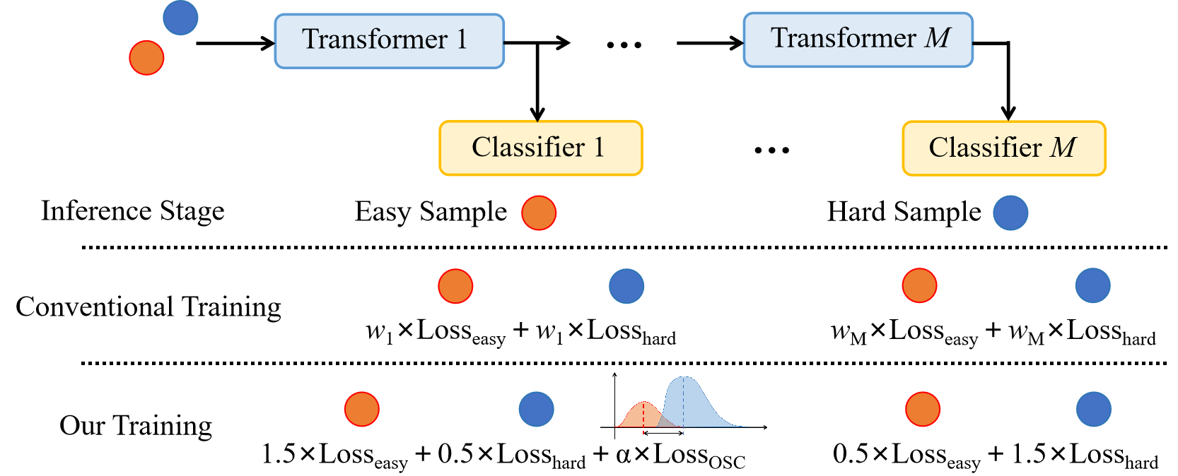
To address these issues, early exiting (Xin et al. 2020; Zhou et al. 2020; Xin et al. 2021; Liao et al. 2021; Sun et al. 2022; Zeng et al. 2024), a kind of adaptive inference strategy, has been proposed to accelerate the inference of PLMs. As illustrated in Figure 2, each intermediate layer of the PLM is coupled with an internal classifier to give an early prediction. This enables the early exiting of samples once the early predictions are sufficiently reliable, eliminating the need for passing them through the entire model. This method employs a sample-wise inference strategy to deal with easy samples with shallow classifiers and process hard samples with deeper classifiers, significantly improving inference efficiency without sacrificing accuracy and alleviating the overthinking problem.
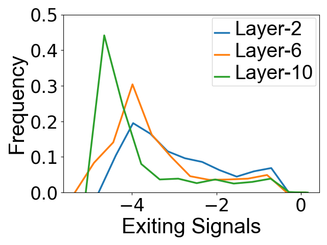
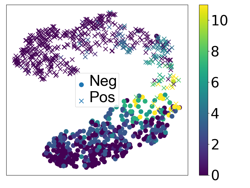
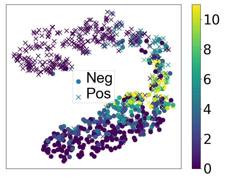
Signal-based early exiting methods (Xin et al. 2020; Liu et al. 2020; Zhou et al. 2020; Schwartz et al. 2020; Li et al. 2021; Liao et al. 2021; Ji et al. 2023; Zhu 2021; Zhu et al. 2021; Gao et al. 2023; Zhang et al. 2023; Zhu et al. 2023; Akbari, Banitalebi-Dehkordi, and Zhang 2022; Xin et al. 2021; Balagansky and Gavrilov 2022) are typical implementations of early exiting, which rely on carefully designed exiting signals (e.g. entropy, energy score, softmax score, and patience) to dynamically adjust the number of executed layers for each sample. The inference process is terminated once the exiting signal meets a certain condition. These methods can easily adapt to various acceleration requirements during inference by simply adjusting the threshold, without incurring additional training costs. However, existing works simply use the (weighted) sum of cross-entropy losses from all classifiers as the training objective, where each classifier treats the loss of both easy and hard samples equally. This treatment ignores the dynamic early exiting behavior during inference (as shown in Figure 1), leading to a gap between training and testing.
To bridge the gap, router-based early exiting methods (Sun et al. 2022; Mangrulkar, MS, and Sembium 2022; Zeng et al. 2024) have been successively proposed. These methods employ a router (e.g. a hash function or a network) to determine the exiting layer of samples during both training and inference, and each sample only incurs a cross-entropy loss at its exiting classifier, ensuring consistency between training and testing. However, router-based early exiting methods fail to meet various acceleration requirements during inference, as a router can only generate a fixed exiting strategy, leading to unadjustable speed-up ratios.
In this paper, we aim to bridge the gap between training and testing while enabling flexible adjustments of the speed-up ratio. To this end, building upon the signal-based early exiting framework, we propose to assign sample-wise weights on the cross-entropy loss of all classifiers, such that each classifier is encouraged to emphasize samples that are more likely to exit at that classifier. Unfortunately, samples exit at different classifiers under various acceleration scenarios, bringing extreme challenges to weight assignment.
To address the challenges, we propose a novel framework of Consistency-Oriented Signal-based Early Exiting (COSEE). Specifically, at each training step, we mimic the test-time early exiting process at multiple randomly selected thresholds to find where the samples tend to exit under different accelerations. Subsequently, we adopt a heuristic sample weighting mechanism (SWM) to assign weights on the cross-entropy loss of each sample across all classifiers, where each sample is emphasized by the classifiers near its exiting layer. Accordingly, we minimize the mean of cross-entropy losses across different thresholds to ensure the model’s generalization ability in various acceleration scenarios. In addition, we further devise an online signal calibration (OSC) objective to generate highly discriminative exiting signals for more reliable exiting decisions, thus encouraging more proper loss weights based on exiting layers.
Our method is simple yet effective. Extensive experiments on the GLUE benchmark demonstrate that our COSEE framework with energy score consistently outperforms the state-of-the-art methods across all tasks, yielding a better trade-off between performance and efficiency with faster convergence speed and negligible additional storage overhead. In addition, an in-depth analysis further confirms the generalization of the COSEE framework on different exiting signals and backbones. Our main contributions can be summarized as follows:
-
•
We disclose that the performance bottleneck of current early exiting methods primarily stems from the challenge of ensuring consistency between training and testing while flexibly adjusting the speed-up ratios.
-
•
We propose a novel Consistency-Oriented Signal-based Early Exiting (COSEE) framework to bridge the gap, which incorporates a sample weighting mechanism (SWM) and an online signal calibration (OSC) objective.
-
•
Extensive experiments verify the effectiveness of our COSEE across multiple exiting signals and backbones.
Code: https://github.com/He-Jianing/COSEE.
2 Preliminaries
In this section, we provide the necessary background for signal-based early exiting 111Related works are detailed in Appendix B..
2.1 Problem Definition
Per Figure 2, given a BERT-style PLM with layers, we denote the hidden states at the th layer as . To enable early exiting during inference on a classification task involving classes, each intermediate layer is equipped with an internal classifier to produce an early prediction , i.e., a probability distribution over the classes. Classifiers in different layers do not share parameters.
2.2 Signal-based Early Exiting
For a given sample , the inference process is terminated once the exiting signal at the current layer meets a certain condition. For exiting signals that exhibit a positive correlation with sample difficulty (e.g. entropy and energy score), early exiting is triggered once the exiting signal falls below a predefined threshold. A higher threshold leads to a higher speed-up ratio and potentially some performance degradation. Conversely, for exiting signals negatively correlated with sample difficulty (e.g. patience and softmax score), the exiting condition is met when the exiting signal surpasses the threshold. A higher threshold leads to a lower speed-up ratio and performance improvements.
2.3 Conventional Training Methods
In current signal-based early exiting methods, a widely used training objective involves the (weighted) sum of cross-entropy losses across all classifiers:
| (1) |
where denotes the cross-entropy loss of the th classifier and denotes the corresponding loss weight. Under Eq.(1), each classifier treats the loss of both easy and hard samples equally, which is inconsistent with the dynamic early exiting behavior during inference.
3 The COSEE Framework
3.1 Framework Overview
We propose a novel Consistency-Oriented Signal-based Early Exiting (COSEE) framework for PLMs, aiming to ensure consistency between training and testing while maintaining flexible adjustments of the speed-up ratio. Figure 2 provides an overview of our framework. We first propose a sample weighting mechanism (SWM) that identifies the potential exiting layer of samples by simulating the test-time early exiting process during training and then uses this information to produce sample-wise loss weights across all classifiers. Additionally, we further devise an online signal calibration (OSC) objective to encourage highly discriminative exiting signals for more reliable exiting decisions, thus ensuring more proper loss weights based on exiting layers. Finally, regarding the exiting signal, we introduce a normalized energy score to align energy distributions across different layers for easy threshold selection. We primarily use it to implement the COSEE framework.
3.2 Sample Weighting Mechanism
Our goal is to identify the potential exiting layer of samples in various acceleration scenarios, and then assign greater weights to the cross-entropy loss of each sample on classifiers closer to its exiting layer. Accordingly, at each training step, all samples are passed through the entire model to generate predictions and exiting signals at all classifiers. Subsequently, we randomly select thresholds and simulate the early exiting process based on exiting signals at each threshold to find where the samples exit. This information is used to produce sample-wise loss weights across all classifiers.
Range for Threshold Selection. For threshold selection, we collect the maximum and minimum values of exiting signals across all layers for training samples within each epoch and use them to create the selection range for the next epoch. We start with the thresholds randomly selected between 0 and 1 in the first epoch.
Weight Assignment. For a given threshold , we impose sample-wise loss weights across all classifiers based on the exiting layer of samples and then compute the classification loss at threshold :
| (2) | |||
| (3) |
where and denote the cross-entropy loss and the loss weight for the th sample at the th classifier respectively, and satisfies . denotes the number of samples. denotes the index of exiting layer for the th sample at threshold , and denotes the decay factor at the th training step. According to Equation 3, classifiers closer to the exiting layer are assigned greater weights compared to those further away, i.e., each sample is emphasized by the classifiers near its exiting layer. Note that the loss weights of classifiers are symmetrical around the exiting layer for easy parameter selection. Different from router-based early exiting methods, which employ one-hot sample-wise loss weights such that each sample only incurs a cross-entropy loss on its exiting classifier, we employ a softer sample weighting mechanism to enable the generality of our COSEE on unseen thresholds.
During the early training stage, unstable exiting layers often lead to fluctuating loss weights, consequently impacting the model’s convergence. To mitigate this problem, we conduct a warm-up operation for the decay factor to gradually increase the impact of the sample’s exiting layers on the loss weights during training:
| (4) |
where is positive, and is the ratio of the current training step to the total training steps.
Classification Objective. To enable various acceleration ratios during inference, the classification objective is defined as the mean of classification losses across all thresholds:
| (5) |
3.3 Online Signal Calibration
While SWM effectively facilitates the training of multi-exit networks, exiting signals may not consistently reflect sample difficulty, particularly during the early training stages. This affects the reliability of exiting decisions, leading to sub-optimal loss weights based on exiting layers. Therefore, we introduce an online signal calibration (OSC) objective to explicitly enlarge the distribution divergence of exiting signals between easy and hard samples. Specifically, for exiting signals that indicate the sample difficulty (e.g. entropy and energy score), our OSC objective is formulated as:
| (6) | |||
| (7) |
where is the signal calibration loss at the th layer. and are the mean of exiting signals on easy and hard samples at the th layer, respectively, and is the margin parameter shared across layers. For exiting signals negatively correlated with sample difficulty (e.g. softmax score), the calculation for in Eq.(7) needs to be replaced with:
| (8) |
Note that we only minimize the signal calibration loss for the first layers, since there is no need to exit at the last layer. Additionally, we define samples as easy or hard depending on whether the internal classifier can predict them correctly, thus the partition may differ across layers.
3.4 Training Objective
The training objective of the COSEE is formulated as the weighted sum of the classification and OSC objective:
| (9) |
where is a hyper-parameter used to balance the classification and OSC objectives. All internal classifiers are jointly trained with the backbone.
3.5 Exiting Signal
Following E-LANG (Akbari, Banitalebi-Dehkordi, and Zhang 2022), we primarily implement our COSEE with the energy-based exiting signal. The energy score is defined as:
| (10) |
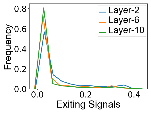
where is the number of classes, and denotes the logit value of sample on class suggested by the th internal classifier . A lower energy score indicates lower sample difficulty. The exiting criterion is met when the energy score falls below a predefined threshold. To align the energy distribution across different layers for threshold selection, we normalize the original energy scores to :
| (11) |
Figure 3 confirms the superiority of the normalized energy score over the original energy score. In this paper, we mainly conduct experiments with the normalized energy score. Nevertheless, we also verify the effectiveness of the COSEE framework on other exiting signals, i.e., entropy and softmax score (see Section 5.2).
4 Experiments
4.1 Tasks and Datasets
4.2 Baselines
We compare our COSEE model with three groups of representative and state-of-the-art baselines.
Backbone. We adopt the widely used BERT-base (Devlin et al. 2019) as the backbone for convincing comparisons.
Budget Exiting. We directly train a BERT-base with 6 layers (BERT-6L) to obtain a speed-up ratio of , establishing a lower bound for early exiting methods as no techniques are employed.
Early Exiting. For signal-based early exiting methods, we choose DeeBERT (Xin et al. 2020), PABEE (Zhou et al. 2020), BERxiT (Xin et al. 2021), LeeBERT (Zhu 2021), GPFEE (Liao et al. 2021), GAML-BERT (Zhu et al. 2021), PALBERT (Balagansky and Gavrilov 2022), and DisentangledEE (Ji et al. 2023). For router-based early exiting methods, we choose state-of-the-art ConsistentEE (Zeng et al. 2024). Notably, some early exiting methods (Sun et al. 2022; Mangrulkar, MS, and Sembium 2022; Zhang et al. 2023; Zhu et al. 2023) are not included due to the difference in backbones. CascadeBERT (Li et al. 2021) and E-LANG (Akbari, Banitalebi-Dehkordi, and Zhang 2022) are excluded for fair comparisons since they implement early exiting within several complete networks instead of a multi-exit network. Refer to Appendix C for more details.
| Dataset | Classes | Train | Test | Task |
|---|---|---|---|---|
| SST-2 | 2 | 67k | 1.8k | Sentiment |
| MRPC | 2 | 3.7k | 1.7k | Paraphrase |
| QQP | 2 | 364k | 391k | Paraphrase |
| MNLI | 3 | 393k | 20k | NLI |
| QNLI | 2 | 105k | 5.4k | QA/NLI |
| RTE | 2 | 2.5k | 3k | NLI |
| Method | RTE | MRPC | QQP | SST-2 | QNLI | MNLI |
|---|---|---|---|---|---|---|
| Acc | F1/Acc/Mean | F1/Acc/Mean | Acc | Acc | Acc | |
| BERT-base | 66.4 (1.00) | 88.9/-/- (1.00) | 71.2/-/- (1.00) | 93.5 (1.00) | 90.5 (1.00) | 84.6 (1.00) |
| BERT-6L† | 63.9 (2.00) | 85.1/78.6/81.9 (2.00) | 69.7/88.3/79.0 (2.00) | 91.0 (2.00) | 86.7 (2.00) | 80.8 (2.00) |
| DeeBERT† | 64.3 (1.95) | 84.4/77.4/80.9 (2.07) | 70.4/88.8/79.6 (2.13) | 90.2 (2.00) | 85.6 (2.09) | 74.4 (1.87) |
| PABEE† | 64.0 (1.81) | 84.4/77.4/80.9 (2.01) | 70.4/88.6/79.5 (2.09) | 89.3 (1.95) | 88.0 (1.87) | 79.8 (2.07) |
| BERxiT | 65.7 (2.17) | 86.2/-/- (2.27) | 70.5/-/- (2.27) | 91.6 (2.86) | 89.6 (1.72) | 82.1 (2.33) |
| LeeBERT | - | 87.1/-/- (1.97) | - | 92.6 (1.97) | - | 83.1 (1.97) |
| GPFEE | 64.5 (2.04) | 87.0/81.8/84.4 (1.98) | 71.2/89.4/80.3 (2.18) | 92.8 (2.02) | 89.8 (1.97) | 83.3 (1.96) |
| GAML-BERT | 64.3 (1.96) | 87.2/-/- (1.96) | 70.9/-/- (1.96) | 92.8 (1.96) | 84.2 (1.96) | 83.3 (1.96) |
| PALBERT‡ | 64.3 (1.48) | -/-/80.7 (1.48) | -/-/79.3 (1.48) | 91.8 (1.48) | 89.1 (1.48) | 83.0 (1.48) |
| DisentangledEE | 66.8 (1.25) | -/-/83.8 (1.25) | -/-/79.4 (1.25) | 92.9 (1.25) | 88.5 (1.25) | 83.0 (1.25) |
| ConsistentEE | 69.0 (1.85) | 89.0/-/- (1.59) | -/89.0/- (1.82) | 92.9 (1.85) | 89.9 (1.72) | 83.4 (1.45) |
| COSEE (ours) | 68.7 (1.96) | 88.0/82.0/85.0 (2.70) | 71.4/89.4/80.4 (2.01) | 93.0 (2.14) | 90.2 (2.56) | 83.4 (1.92) |
4.3 Experimental Settings
Measurement. Since the runtime is unstable across different runs, following Zhang et al. (2022) and Liao et al. (2021), we utilize the saved layers to measure the speed-up ratio:
| (12) |
where is the total number of layers and is the number of samples exiting from the th layer. According to Xin et al. (2020), this metric is proportional to actual runtime.
Training. Our implementation is based on Hugging Face’s Transformers (Wolf et al. 2020). Each internal classifier consists of a single linear layer. We mainly implement our COSEE framework with the normalized energy score if not specified. We also conduct experiments with entropy and softmax scores for generalization analysis. Following the previous work (Zhou et al. 2020; Zhang et al. 2022; Liao et al. 2021), we perform a grid search over learning rates of {1e-5, 2e-5, 3e-5, 5e-5}, batch sizes of , values in Eq.(9) of , and values in Eq.(4) of . We set to in Eq.(7) and to in Eq.(5). The maximum sequence length is fixed at . We employ a linear decay learning rate scheduler and the AdamW optimizer (Loshchilov and Hutter 2019). We conduct experiments on two RTX4090 GPUs with 24GB.
Inference. Following previous work (Zhang et al. 2022; Liao et al. 2021), we adopt a batch size of for inference, emulating a typical industry scenario where requests from various users arrive one by one. For fair comparisons, we carefully adjust the threshold for each task to achieve a similar speed-up ratio as the baseline methods (approximately ) and further compare the trade-off between task performance and inference efficiency.
4.4 Overall Performance Comparison
Table 2 reports the test results of each early exiting method on the GLUE benchmark with BERT-base as the backbone model. The speed-up ratio is approximately (±38). Overall, our COSEE framework with normalized energy score demonstrates a superior performance-efficiency trade-off across different tasks compared to the baseline methods, which verifies the effectiveness of our design. Notably, our COSEE can even outperform the original BERT-base on RTE and QQP tasks, indicating that our method can effectively alleviate the overthinking problem of PLMs. This suggests that, for easy samples, predictions from intermediate layers may outperform those from the final layer. Our method enables easy samples to exit at shallow classifiers, thereby reducing the inference time while maintaining or even improving the task performance. Besides, our method can save training costs (see Section 4.5) and introduce negligible additional storage overhead (see Section 5.3). We also explore the impact of hyperparameters (see Appendix A) and analyze the failure cases statistically (see Appendix D).
Although using energy scores and BERT-base in the primary experiments, we also verify the generality of COSEE on various exiting signals and backbones (see Section 5.2).
4.5 Ablation Studies
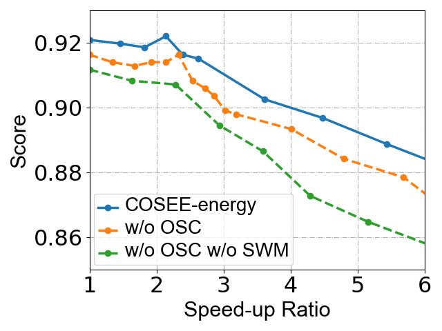
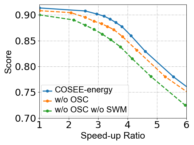
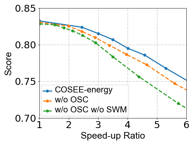
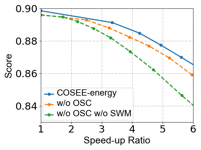
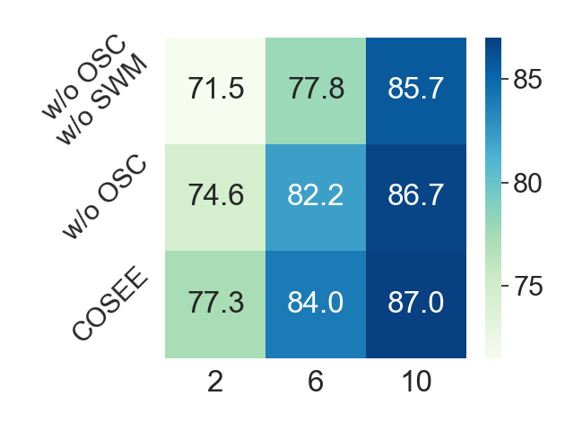
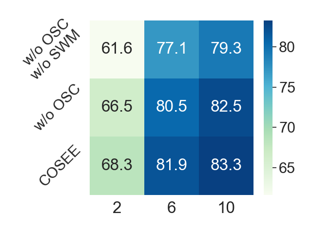
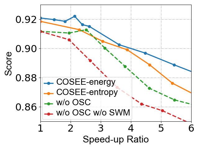
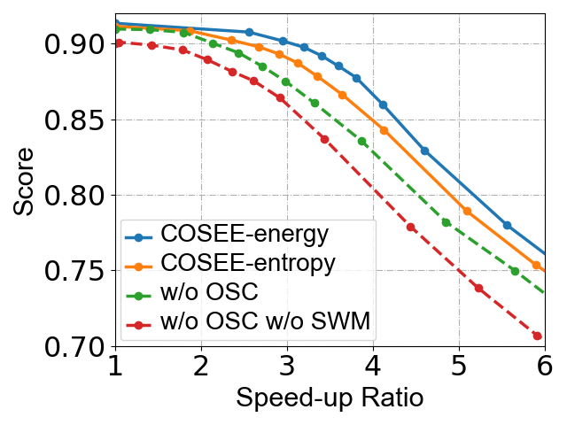
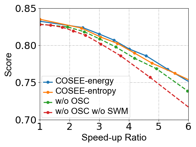
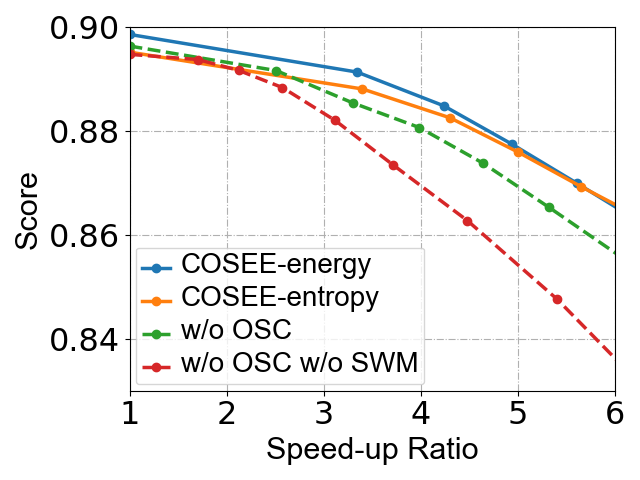
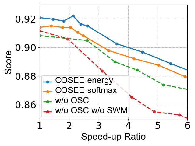
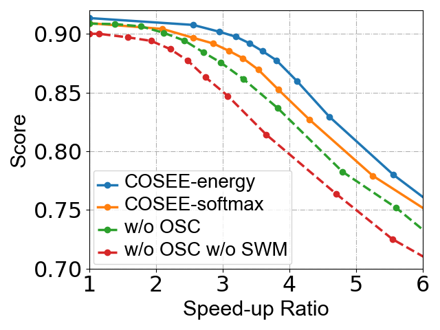
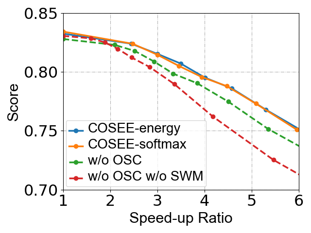
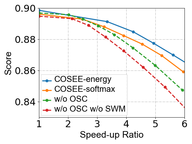
Performance-Efficiency Trade-Off. To investigate the effectiveness of SWM and OSC, we plot the performance-efficiency trade-off curves of models trained using different methods on a representative subset of GLUE, as shown in Figure 4. We can observe both SWM and OSC significantly improve the performance of early exiting across all tasks, especially under high speed-up ratios. This confirms the advantage of our COSEE under high acceleration scenarios, indicating the proposed SWM and OSC effectively facilitate the training of internal classifiers, particularly shallow ones.
Evaluation of Exiting Signals. Difficulty Inversion Score (DIS) is first proposed by Li et al. (2021), an evaluation metric for exiting signals. A higher value indicates a greater correlation between the exiting signal and sample difficulty, thus enabling more reliable exiting decisions. Figure 5 illustrates the DIS of exiting signals generated by different models on SST-2 and QNLI tasks. The results indicate that OSC explicitly enhances the correlation between the exiting signal and sample difficulty by enlarging the distribution divergence of exiting signals between easy and hard samples. Meanwhile, SWM encourages highly discriminative exiting signals by enabling each classifier to emphasize a subset of samples with certain difficulty levels. Also, it is noticeable that the improvements brought by SWM and OSC appear to be significant on shallow layers, which aligns with the observation shown in Figure 4. This is due to the constrained capability of shallow classifiers, which allows for greater potential for improvements in training than deep classifiers.
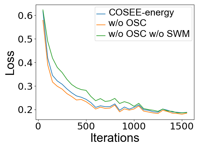
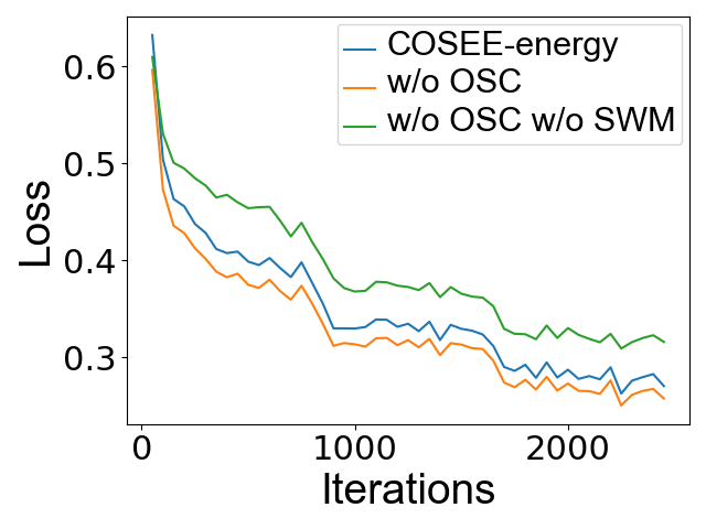
Training Curves. To further explore the convergence speed of our COSEE during training, we plot the model’s training curves across different training methods on SST-2 and QNLI tasks, as shown in Figure 6. The results indicate that the proposed SWM effectively accelerates the model’s convergence during training. We attribute this to SWM’s ability to reduce data complexity during training by enabling each classifier to emphasize a different subset of samples. Additionally, we can observe that incorporating the OSC objective can slightly impact the model’s convergence speed. Nevertheless, our COSEE framework still maintains an advantage over the vanilla training method.
5 In-depth Analysis
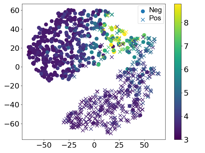
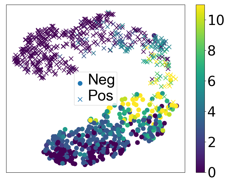
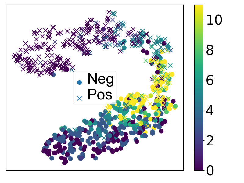
5.1 Visualization of Sample Exiting Layers
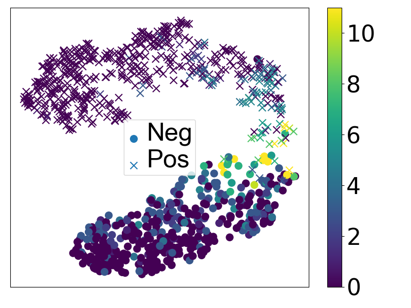
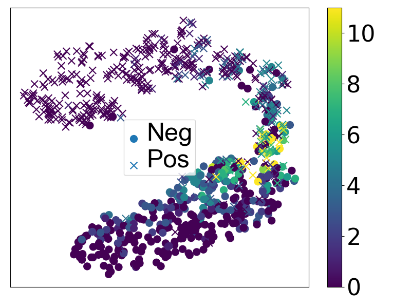
To examine the consistency between training and testing under our COSEE framework, we visualize the exiting layer distribution in training and development sets at various thresholds, respectively. Figure 7 shows the visualization results for the SST-2 task. As we can see, training and development sets exhibit a consistent exiting layer distribution across different thresholds, which verifies the interpretability of our design. Additionally, we can observe that samples near the classification boundary (hard samples) tend to exit at deep classifiers while samples far from the classification boundary (easy samples) tend to exit at shallow classifiers. Furthermore, increasing the threshold will cause a decrease in exiting layers, thus achieving a higher speed-up ratio. These observations align with our intuitive understanding.
5.2 Generality of the COSEE Framework
In this subsection, we explore the generality of our method on various exiting signals and backbones. The experiments are conducted on a representative subset of GLUE.
Figure 8 and Figure 9 present the experimental results of our COSEE framework with entropy and softmax scores, respectively. The results demonstrate the generality of our COSEE framework across various exiting signals. In addition, COSEE with energy scores outperforms COSEE with entropy or softmax scores on most tasks (SST-2, QNLI, and QQP). We speculate that this is because the energy score is more reliable in distinguishing easy and hard samples when compared to entropy and softmax scores. Akbari, Banitalebi-Dehkordi, and Zhang (2022) confirmed this statement through theoretical derivation. Therefore, we primarily implement COSEE with energy scores in this paper.
Table 3 presents the performance comparison with backbone ALBERT-base. We observe that our COSEE with energy outperforms competitive baseline methods on most tasks, demonstrating its generality across different PLMs.
| Method | Speed-up | QQP | SST-2 | QNLI | MNLI | AVG |
|---|---|---|---|---|---|---|
| ALBERT-base† | 1.00 | 79.6 | 93.3 | 92.0 | 85.2 | 87.5 |
| PABEE† | 1.95 | 79.8 | 92.4 | 90.9 | 84.2 | 86.8 |
| PALBERT | 1.21 | 79.1 | 91.4 | 90.9 | 83.2 | 86.2 |
| DisentangledEE | 1.26 | 79.3 | 92.2 | 91.0 | 83.5 | 86.5 |
| COSEE-energy | 2.12 | 79.6 | 92.9 | 91.8 | 84.8 | 87.3 |
5.3 Storage Costs Analysis
Table 4 compares the parameter volumes of our COSEE model with those of the original BERT-base. We observe that our COSEE model only requires less than 0.03 additional parameters due to the incorporation of internal classifiers. Additionally, it is noteworthy that the proposed SWM is parameter-free, yet it can effectively generate proper loss weights for each sample to facilitate the training of a multi-exit network.
| Model | #Params | |
|---|---|---|
| BERT-base | 109.48M | 109.48M |
| COSEE | +16.92K | +25.38K |
6 Conclusion
In this paper, we point out that the performance bottleneck of existing early exiting methods primarily lies in the challenge of ensuring consistency between training and testing while enabling flexible adjustments of the speed-up ratio. To remedy this, we propose COSEE, which mimics the test-time early exiting process under various acceleration scenarios based on calibrated exiting signals and then produces the sample-wise loss weights at all classifiers according to the sample’s exiting layer. Our framework is both simple and intuitive. Extensive experiments on the GLUE benchmark demonstrate the superiority and generality of our framework across various exiting signals and backbones.
Acknowledgements
This work was supported by the National Natural Science Foundation of China (Grant No. 62376198), the National Key Research and Development Program of China (Grant No. 2022YFB3104700), and the Shanghai Baiyulan Pujiang Project (No. 08002360429).
References
- Akbari, Banitalebi-Dehkordi, and Zhang (2022) Akbari, M.; Banitalebi-Dehkordi, A.; and Zhang, Y. 2022. E-lang: Energy-based joint inferencing of super and swift language models. arXiv preprint arXiv:2203.00748.
- Balagansky and Gavrilov (2022) Balagansky, N.; and Gavrilov, D. 2022. Palbert: Teaching albert to ponder. Advances in Neural Information Processing Systems, 35: 14002–14012.
- Devlin et al. (2019) Devlin, J.; Chang, M.; Lee, K.; and Toutanova, K. 2019. BERT: Pre-training of Deep Bidirectional Transformers for Language Understanding. In NAACL-HLT (1), 4171–4186. Association for Computational Linguistics.
- Gao et al. (2023) Gao, X.; Zhu, W.; Gao, J.; and Yin, C. 2023. F-PABEE: flexible-patience-based early exiting for single-label and multi-label text classification tasks. In ICASSP 2023-2023 IEEE International Conference on Acoustics, Speech and Signal Processing (ICASSP), 1–5. IEEE.
- Ji et al. (2023) Ji, Y.; Wang, J.; Li, J.; Chen, Q.; Chen, W.; and Zhang, M. 2023. Early exit with disentangled representation and equiangular tight frame. In Findings of the Association for Computational Linguistics: ACL 2023, 14128–14142.
- Kaya, Hong, and Dumitras (2019) Kaya, Y.; Hong, S.; and Dumitras, T. 2019. Shallow-Deep Networks: Understanding and Mitigating Network Overthinking. In ICML, volume 97 of Proceedings of Machine Learning Research, 3301–3310. PMLR.
- Lan et al. (2020) Lan, Z.; Chen, M.; Goodman, S.; Gimpel, K.; Sharma, P.; and Soricut, R. 2020. ALBERT: A Lite BERT for Self-supervised Learning of Language Representations. In ICLR. OpenReview.net.
- Li et al. (2021) Li, L.; Lin, Y.; Chen, D.; Ren, S.; Li, P.; Zhou, J.; and Sun, X. 2021. CascadeBERT: Accelerating Inference of Pre-trained Language Models via Calibrated Complete Models Cascade. In EMNLP (Findings), 475–486. Association for Computational Linguistics.
- Liao et al. (2021) Liao, K.; Zhang, Y.; Ren, X.; Su, Q.; Sun, X.; and He, B. 2021. A Global Past-Future Early Exit Method for Accelerating Inference of Pre-trained Language Models. In NAACL-HLT, 2013–2023. Association for Computational Linguistics.
- Liu et al. (2020) Liu, W.; Zhou, P.; Wang, Z.; Zhao, Z.; Deng, H.; and Ju, Q. 2020. FastBERT: a Self-distilling BERT with Adaptive Inference Time. In ACL, 6035–6044. Association for Computational Linguistics.
- Liu et al. (2019) Liu, Y.; Ott, M.; Goyal, N.; Du, J.; Joshi, M.; Chen, D.; Levy, O.; Lewis, M.; Zettlemoyer, L.; and Stoyanov, V. 2019. RoBERTa: A Robustly Optimized BERT Pretraining Approach. CoRR, abs/1907.11692.
- Loshchilov and Hutter (2019) Loshchilov, I.; and Hutter, F. 2019. Decoupled Weight Decay Regularization. In ICLR (Poster). OpenReview.net.
- Mangrulkar, MS, and Sembium (2022) Mangrulkar, S.; MS, A.; and Sembium, V. 2022. BE3R: BERT based Early-Exit Using Expert Routing. In Proceedings of the 28th ACM SIGKDD Conference on Knowledge Discovery and Data Mining, 3504–3512.
- Radford et al. (2019) Radford, A.; Wu, J.; Child, R.; Luan, D.; Amodei, D.; Sutskever, I.; et al. 2019. Language models are unsupervised multitask learners. OpenAI blog, 1(8): 9.
- Schwartz et al. (2020) Schwartz, R.; Stanovsky, G.; Swayamdipta, S.; Dodge, J.; and Smith, N. A. 2020. The Right Tool for the Job: Matching Model and Instance Complexities. In ACL, 6640–6651. Association for Computational Linguistics.
- Sun et al. (2022) Sun, T.; Liu, X.; Zhu, W.; Geng, Z.; Wu, L.; He, Y.; Ni, Y.; Xie, G.; Huang, X.; and Qiu, X. 2022. A Simple Hash-Based Early Exiting Approach For Language Understanding and Generation. In ACL (Findings), 2409–2421. Association for Computational Linguistics.
- Wang et al. (2019) Wang, A.; Singh, A.; Michael, J.; Hill, F.; Levy, O.; and Bowman, S. R. 2019. GLUE: A Multi-Task Benchmark and Analysis Platform for Natural Language Understanding. In ICLR (Poster). OpenReview.net.
- Wolf et al. (2020) Wolf, T.; Debut, L.; Sanh, V.; Chaumond, J.; Delangue, C.; Moi, A.; Cistac, P.; Rault, T.; Louf, R.; Funtowicz, M.; Davison, J.; Shleifer, S.; von Platen, P.; Ma, C.; Jernite, Y.; Plu, J.; Xu, C.; Scao, T. L.; Gugger, S.; Drame, M.; Lhoest, Q.; and Rush, A. M. 2020. Transformers: State-of-the-Art Natural Language Processing. In EMNLP (Demos), 38–45. Association for Computational Linguistics.
- Xin et al. (2020) Xin, J.; Tang, R.; Lee, J.; Yu, Y.; and Lin, J. 2020. DeeBERT: Dynamic Early Exiting for Accelerating BERT Inference. In ACL, 2246–2251. Association for Computational Linguistics.
- Xin et al. (2021) Xin, J.; Tang, R.; Yu, Y.; and Lin, J. 2021. BERxiT: Early Exiting for BERT with Better Fine-Tuning and Extension to Regression. In EACL, 91–104. Association for Computational Linguistics.
- Zeng et al. (2024) Zeng, Z.; Hong, Y.; Dai, H.; Zhuang, H.; and Chen, C. 2024. ConsistentEE: A Consistent and Hardness-Guided Early Exiting Method for Accelerating Language Models Inference. In Proceedings of the AAAI Conference on Artificial Intelligence, volume 38, 19506–19514.
- Zhang et al. (2023) Zhang, J.; Tan, M.; Dai, P.; and Zhu, W. 2023. Leco: Improving early exiting via learned exits and comparison-based exiting mechanism. In Proceedings of the 61st Annual Meeting of the Association for Computational Linguistics (Volume 4: Student Research Workshop), 298–309.
- Zhang et al. (2022) Zhang, Z.; Zhu, W.; Zhang, J.; Wang, P.; Jin, R.; and Chung, T. 2022. PCEE-BERT: Accelerating BERT Inference via Patient and Confident Early Exiting. In NAACL-HLT (Findings), 327–338. Association for Computational Linguistics.
- Zhou et al. (2020) Zhou, W.; Xu, C.; Ge, T.; McAuley, J. J.; Xu, K.; and Wei, F. 2020. BERT Loses Patience: Fast and Robust Inference with Early Exit. In NeurIPS.
- Zhu (2021) Zhu, W. 2021. LeeBERT: Learned early exit for BERT with cross-level optimization. In Proceedings of the 59th Annual Meeting of the Association for Computational Linguistics and the 11th International Joint Conference on Natural Language Processing (Volume 1: Long Papers), 2968–2980.
- Zhu et al. (2023) Zhu, W.; Wang, P.; Ni, Y.; Xie, G.; and Wang, X. 2023. BADGE: speeding up BERT inference after deployment via block-wise bypasses and divergence-based early exiting. In Proceedings of the 61st Annual Meeting of the Association for Computational Linguistics (Volume 5: Industry Track), 500–509.
- Zhu et al. (2021) Zhu, W.; Wang, X.; Ni, Y.; and Xie, G. 2021. GAML-BERT: improving BERT early exiting by gradient aligned mutual learning. In Proceedings of the 2021 Conference on Empirical Methods in Natural Language Processing, 3033–3044.
Appendix A Parameter Sensitivity Analysis
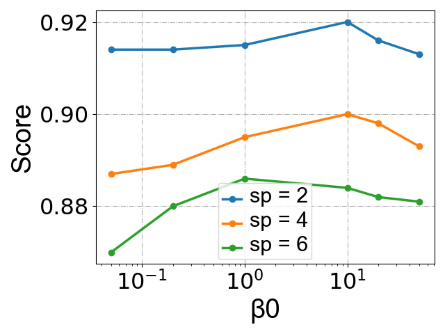
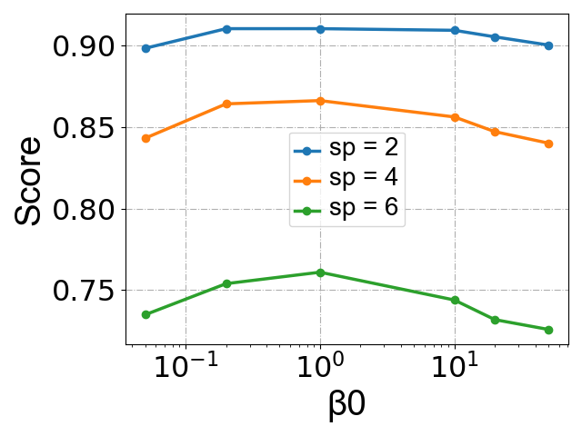
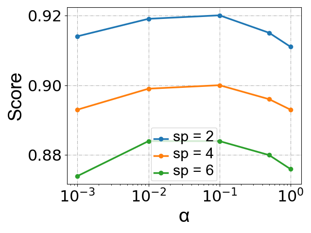
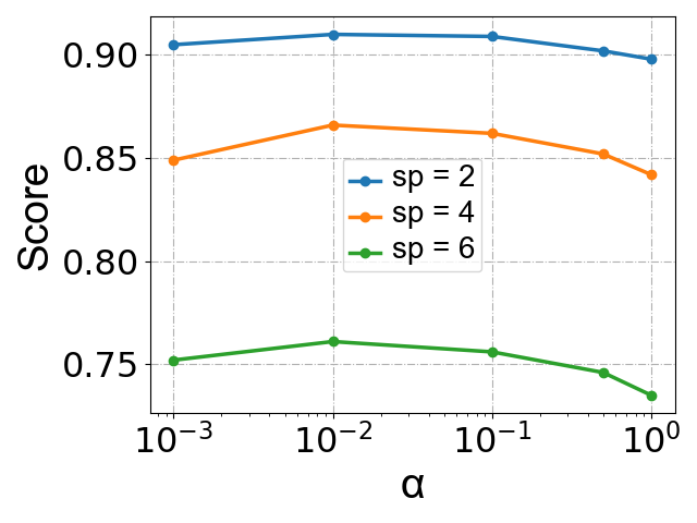
In this section, we further investigate the impact of four parameters on task performance under different speed-up ratios. Figure 10 shows the experimental results on SST-2 and QNLI tasks.
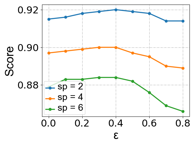
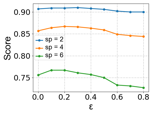
Impact of . The parameter in Eq.(4) is utilized to adjust the distribution of loss weights across all classifiers. As shown in Figure 10(a) and Figure 10(b), both excessively large and small values of can impair the acceleration performance of the COSEE model, and the optimal value differs across tasks. Additionally, under high acceleration scenarios, the performance improvements brought by SWM are particularly significant, which is consistent with the observations in Figure 4 and Figure 5.
Impact of . The parameter in Eq.(9) balances the classification objective and OSC objective during training. The results depicted in Figure 10(c) and Figure 10(d) indicate that the acceleration performance of our COSEE model is not significantly affected by selection, and an value between 0.01 and 0.1 can always lead to satisfactory performance across different tasks. Moreover, an excessively large value can lead to performance degradation. We attribute this to an overemphasis on the OSC objective, which interferes with the optimization of task performance.
Impact of . The parameter in Eq.(7) is utilized to regulate the distribution divergence of exiting signals between easy and hard samples. As shown in Figure 10(e) and Figure 10(f), an value between 0.1 and 0.4 can always lead to satisfactory performance across different tasks. Consequently, we fix the value at 0.3 to simplify the parameter selection.
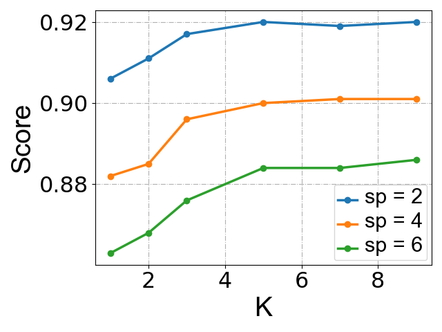
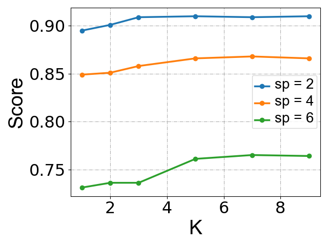
Impact of . The parameter in Eq.(5) determines the number of thresholds randomly selected at each training step. The results in Figure 10(g) and Figure 10(h) show that, as the value of increases, the task performance exhibits a consistent pattern of initially increasing and then stabilizing under various speed-up ratios. This aligns with our intuition as selecting diverse thresholds during training is crucial for enabling models to meet different acceleration requirements during inference. We fix the value at 5 for all tasks for computational efficiency.
Appendix B Related Works
The early exiting methods applied to PLMs can be roughly divided into two categories: signal-based early exiting and router-based early exiting.
B.1 Signal-based Early Exiting
Signal-based early exiting methods dynamically adjust the number of executed layers for each sample based on the exiting signal, enabling samples to exit early during inference once the exiting conditions are satisfied.
According to the type of exiting signal, signal-based early exiting can be further categorized into score-based early exiting, patience-based early exiting, and learning-based early exiting. Score-based early exiting methods (Xin et al. 2020; Liu et al. 2020; Schwartz et al. 2020; Akbari, Banitalebi-Dehkordi, and Zhang 2022; Li et al. 2021; Liao et al. 2021) leverage the entropy, softmax score, or energy score to capture the uncertainty of early predictions. Early exiting is triggered once the entropy or energy score (softmax score) falls below (surpasses) the predefined threshold. Patience-based early exiting methods (Zhou et al. 2020; Gao et al. 2023; Zhang et al. 2023; Zhu et al. 2023; Ji et al. 2023; Zhu 2021; Zhu et al. 2021) utilize the cross-layer consistency as the exiting signal. The exiting criterion is met when enough (i.e. greater than the threshold) consecutive internal classifiers agree with each other. Lastly, learning-based early exiting methods (Xin et al. 2021; Balagansky and Gavrilov 2022) leverage neural networks to generate exiting signals for exit decision-making.
According to the training of multi-exit networks, some studies (Xin et al. 2020; Schwartz et al. 2020; Xin et al. 2021; Balagansky and Gavrilov 2022) minimize the sum of cross-entropy losses across all classifiers, whereas other studies (Zhou et al. 2020; Liao et al. 2021; Zhu 2021; Zhu et al. 2021) minimize the weighted sum of cross-entropy losses across all classifiers. In addition, LeeBERT (Zhu 2021) and GAML-BERT (Zhu et al. 2021) employ the cross-layer distillation objective to further enhance the training of internal classifiers.
Signal-based early exiting can easily adapt to different acceleration requirements by simply adjusting the threshold, without incurring additional training costs. However, in current studies, each classifier treats all samples equally during training, which neglects the dynamic early exiting behaviors across different samples, leading to a gap between training and testing.
B.2 Router-based Early Exiting
Router-based early exiting methods employ a router to determine exiting in both the training and inference phases. Some studies (Sun et al. 2022; Mangrulkar, MS, and Sembium 2022) utilize a hash function or a network to assign the exiting layer for each sample. ConsistentEE (Zeng et al. 2024) employs reinforcement learning to train a policy network for exit decision-making.
These methods perform early exiting during training, and each sample only incurs a cross-entropy loss at its exiting classifier. This treatment effectively ensures consistency between training and testing. However, router-based early exiting methods fail to meet various acceleration requirements during inference, as a router (a hash function or a trained network) can only generate a fixed exiting strategy, leading to unadjustable speed-up ratios.
This work proposes a novel signal-based early exiting framework to ensure consistency between training and testing while enabling flexible adjustment of the speed-up ratio.
Appendix C Baseline Competitors
In this section, we introduce the comparative early exiting methods in our experiments in detail.
C.1 Signal-based Early Exiting
According to the exiting signal, DeeBERT and GPFEE leverage entropy to capture the uncertainty of early predictions. Early exiting is triggered once the entropy falls below the predefined threshold. PABEE, LeeBERT, GAML-BERT, and DisentangledEE employ the cross-layer consistency as the exiting signal. The exiting criterion is met when enough (i.e. greater than the threshold) consecutive internal classifiers agree with each other. BERxiT learns to score the correctness of early predictions through a network. The inference process is terminated when the correctness score surpasses the threshold. PALBERT (Balagansky and Gavrilov 2022) performs early exiting once the cumulative distribution function of the exiting layer’s probability distribution provided by neural networks exceeds the threshold.
According to the architecture or training objective of multi-exit networks, DeeBERT, PABEE, BERxiT and PALBERT minimize the cross-entropy losses for all classifiers. LeeBERT and GAML-BERT introduce the cross-layer distillation objective to encourage mutual learning among different classifiers. GPFEE integrates past and future states as inputs for each classifier, providing more reliable early predictions. DisentangledEE introduces an adapter to decouple the generic language representation learning and task-specific feature extraction and proposes a non-parametric simplex equiangular tight frame classifier for improvement.
C.2 Router-based Early Exiting
ConsistentEE employs reinforcement learning to train a policy network for exit decision-making and minimizes the cross-entropy loss for each sample only at its exiting classifier during training.
Appendix D Statistics of Failure Cases
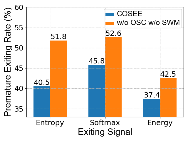
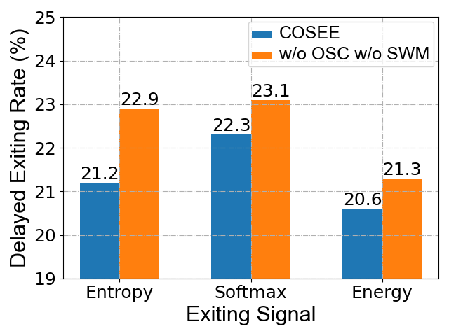
In this section, we conduct a statistical analysis of failure cases to assess the reliability of exiting decisions. There are two types of failure cases: first, the model may prematurely emit samples with incorrect early predictions by underestimating their difficulty, which degrades task performance; second, the model may delay the exiting of samples with correct early predictions by overestimating their difficulty, which prolongs inference time. Both types can negatively impact the model’s performance-efficiency trade-off. Accordingly, we define two metrics to statistically analyze these two types of failure cases, respectively.
-
•
Premature Exiting Rate: the ratio of ”exit” decisions made when the internal classifier predicts incorrectly.
-
•
Delayed Exiting Rate: the ratio of ”continue” decisions made when the internal classifier predicts correctly.
Exiting decisions are considered reliable only when both the Premature and Delayed Exiting Rate are sufficiently low. Figure 11 presents the failure cases statistics for COSEE and the conventional training method under various exiting signals in the SST-2 task. We observe that, compared to the conventional training method, our COSEE significantly reduces both the Premature and Delayed Exiting Rate across various exiting signals. This suggests that our COSEE facilitates the reliability of exiting decisions during inference by improving the training of multi-exit networks.