Logic-Constrained Shortest Paths for Flight Planning

Logic-Constrained Shortest Paths for Flight Planning

Abstract

The Logic-Constrained Shortest Path Problem (LCSP) combines a one-to-one shortest path problem with satisfiability constraints imposed on the routing graph. This setting arises in flight planning, where air traffic control (ATC) authorities are enforcing a set of traffic flow restrictions (TFRs) on aircraft routes in order to increase safety and throughput. We propose a new branch and bound-based algorithm for the LCSP.

The resulting algorithm has three main degrees of freedom: the node selection rule, the branching rule and the conflict. While node selection and branching rules have been long studied in the MIP and SAT communities, most of them cannot be applied out of the box for the LCSP. We review the existing literature and develop tailored variants of the most prominent rules. The conflict, the set of variables to which the branching rule is applied, is unique to the LCSP. We analyze its theoretical impact on the B&B algorithm.

In the second part of the paper, we show how to model the Flight Planning Problem with TFRs as an LCSP and solve it using the branch and bound algorithm. We demonstrate the algorithm’s efficiency on a dataset consisting of a global flight graph and a set of around 20000 real TFRs obtained from our industry partner Lufthansa Systems GmbH. We make this dataset publicly available. Finally, we conduct an empirical in-depth analysis of node selection rules, branching rules and conflicts. Carefully choosing an appropriate combination yields an improvement of an order of magnitude compared to an uninformed choice.

Index terms— Flight Planning, Traffic Flow Restriction, Shortest Path, Logical Constraints, Branch and Bound

Declaration of interest— none

1 Introduction

The problem of routing an aircraft from a source airport to a target airport while minimizing the operational cost is called the Flight Planning Problem (FPP) and its multiple variants and constraints have been thoroughly studied in the literature [1, 2, 3, 4, 5, 6, 7, 8]. FPP is a time-dependent one-to-one shortest path problem defined on a directed graph called an airway network with arc cost functions that depend on fuel consumption, weather, and overflight costs. The two input airports are called an origin-destination pair or, in short, an OD pair.

A cornerstone for commercial aircraft routing systems is the handling of so-called Traffic Flow Restrictions (TFR) imposed on the airway network. A TFR can, for example, specify that any aircraft that enters Germany using a node on the frontier with Switzerland and heads to the southern part of the UK must leave the European mainland via Bruges. This mandatory rule gives the air traffic controllers some predictability and enables a single controller to survey more aircraft simultaneously. That is why Flight Planning solvers need to compute optimal routes that adhere to the TFR system. Otherwise, the computed routes are not accepted by air traffic controllers.

TFRs are stated as propositional formulae that can be formulated in disjunctive normal form (DNF) where the literals correspond to nodes and arcs in the airway network. Currently, there are around $20\,000$ active TFRs that are updated every day. The TFR example above exhibits a general algorithmic problem arising in TFR handling: the resolution (after Bruges) of a rule can be geographically far away from its activation (entering Germany via Switzerland). Suppose two subpaths $p$ and $q$ meet in Germany while computing a route from Croatia to the UK. Assume $p$ entered Germany via Switzerland and $q$ did not. Moreover, let $q$ be more expensive than $p$ when both paths meet. State-of-the-art shortest path algorithms would at this point discard $q$ because it is more expensive. In our situation, however, we cannot discard $q$ because $p$ is forced to leave the European mainland via Bruges and this might result in a more expensive route at the end. The high amount of TFRs in real-world scenarios thus invalidates solution approaches in which every subpath has a logical subsystem attached to it [5, 4, 7]. In such approaches, subpaths only become comparable via their cost when their logical systems involve the same TFRs. This causes an exponential number of incomparable paths to be stored until shortly before the target airport is reached, only to keep a single path as an optimal solution.

In this paper, we model the flight planning problem with traffic flow restrictions as a Logic-Constrained Shortest Path Problem (LCSP) and suggest a branch and bound (B&B) algorithm to solve it. In every node of the B&B tree, an FPP instance is solved without considering TFRs. The resulting path is then evaluated w.r.t. the TFRs and the resulting logical infeasibilities are used to branch. This black box approach circumvents the above-mentioned memory consumption and running time issues caused by the incomparability of paths. Across world regions, the distribution of TFRs is heterogeneous. For example, there is a large amount of TFRs in Central Europe and the Persian Gulf but very few in Australia or Southern Africa (cf. Fig. 1). For many OD pairs, our algorithm thus solves the LCSP instances in the root node of the B&B tree creating very little overhead compared to a standard FPP search.

Since our approach repeatedly recomputes shortest paths, we can make use of one of the several dynamic shortest path algorithms in the literature [9, 10, 11, 12, 13, 14, 15]. These approaches enable us to warm-start the shortest-path queries in the B&B tree. They are meant to avoid the re-exploration of the search space (graph) on, e.g., a route from Australia to Europe, if the only TFR violations are close to the destination airport.

Figure 1: The upper figure depicts all 19300 airway segments that are contained in at least one TFR. We can see that adherence to the North Atlantic Organized Track System is enforced using TFRs. The lower figure shows all 11386 waypoints that are contained either directly or via an airway segment in at least one TFR. A density distribution of these waypoints in the projective plane was calculated using Gaussian kernel density estimation. It was used to color the waypoints with blue indicating areas with a low density of TFRs and red indicating areas with a high density of TFRs.

Shortest path problems with logical constraints have been studied on occasion in the literature. Aloul et al. [16] propose a pseudo-Boolean formulation for the shortest path problem that lends itself to the integration of logical constraints. They obtain poor run times even on small graphs and even in the absence of logical constraints. Nishino et al. [17] propose a framework in which logical constraints are formulated as binary decision diagrams (BDDs). TFRs are, however, not given as BDDs but as propositional formulae and even a minimum size BDD can be exponential in the size of the propositional formula [18]. The formal language constrained shortest path problems (FLCSP) [19] demands that the shortest path is accepted by a formal language. For context-free languages, it can be solved in polynomial time by dynamic programming, while it is NP-hard for context-sensitive languages [19]. Euler et al. [20] combine the (regular) formal language constrained shortest path problem and a non-linear resource constrained shortest path problem [21] to compute public routes subject to constraints imposed by fares.

The LCSP is a generalization of the path with forbidden pairs problem (FPSP) and hence NP-hard [22], even on directed acyclic graphs.

1.1 Contribution

In this paper, we make three contributions. First, we formalize the Logic-Constrained Shortest Path Problem on acyclic directed graphs and present a B&B-based algorithm to solve it. Second, we adapt several branching strategies from the MIP and SAT communities for the LCSP and evaluate their performance on a large-scale flight planning problem. Third, we make the problem data available to the community. It consists of a realistic world-wide airway network, its corresponding set of $18\,239$ TFRs, and a simple aircraft model that ensures that realistic optimal routes are computed.

Remark 1.1.

Airway networks are not acyclic. However, given an OD-pair, it is a common technique in flight planning to make the routing subgraph acyclic, as arcs pointing in the direction of the departure airport are not needed. This preprocessing is handy when dealing with LCSP instances. We need to rule out that paths resolve logical constraints by flying cycles. This is certainly not allowed and would undermine the Air Traffic Controller’s motivation to file certain TFRs. For example, if flying over a direct connection between two nodes is only allowed after $8$ pm, an aircraft must not cycle around until the so called DIRECT is enabled. In the following, we hence consider all directed graphs to be acyclic.

2 An Algorithm for the Logic-Constrained Shortest Path Problem

We consider a directed acyclic graph (DAG) $G=(V,A)$ and a propositional formula $\Phi$ over a set of propositional variables $X$. Some variables $Y\subseteq X$ correspond to arcs in $G$ via a bijection $\rho:A\to Y$. We call variables in $Y$ graph variables and variables in $Z:=X\backslash Y$ free variables.

2.1 Notation for Propositional Logic

W.l.o.g., we assume $\Phi$ to be in conjunctive normal form (CNF), i.e., $\Phi$ is a conjunction of clauses and each clause is a disjunction of literals $l\in\bigcup_{x\in X}\{x,\neg x\}$. This assumption is justified since any propositional formula can be transformed into a CNF in linear time using the Tseitin encoding [23]. The resulting formula contains additional variables representing subformulae, but the size increase is linear w.r.t. the original size of $\Phi$. Indexing clauses with $I$ and the literals in a clause $i\in I$ with $J_{i}$, $\Phi$ can be written in set notation as

$$\Phi=\left\{\left\{l_{ij}:j\in J_{i}\right\}\ :\ i\in I\right\}.$$ (1)

A set of literals $T\subseteq\bigcup_{x\in X}\{x,\neg x\}$ is called an assignment $T$ if it does not contain a contradiction, i.e., for all $l\in T$ we have $\neg l\not\in T$. An assignment assigns truth values to the variables $X$, i.e., $x\in X$ is assigned true if $x\in T$ and assigned false if $\neg x\in T$. If neither $x\in T$ nor $\neg x\in T$, the variable $x$ is called unassigned. An assignment $T$ is complete if it assigns all variables, i.e, $|T|=|X|$.

Using the notation from [24], we may condition $\Phi$ on some literal $l$ by letting

$$\Phi|l:=\left\{\alpha\backslash\{\neg l\}\ :\ \alpha\in\Phi,l\not\in\alpha\right\},$$ (2)

i.e., in $\Phi|l$ all clauses containing $l$ are deleted and $\neg l$ is removed from the remaining ones. All other clauses remain unchanged.

For an assignment $T$, we let $\Phi|T:=\Phi|l_{1}|\dots|l_{k}$ for any ordering $(l_{1},\dots,l_{k})$ of $T$. The expression is well-defined, since conditioning is order-invariant.

Finally, an assignment $T$ satisfies $\Phi$ if $\Phi|T=\emptyset$. Specifically, it satisfies a clause $\alpha$ if $\{\alpha\}|T=\emptyset$. If there is no assignment that satisfies $\Phi$, it is unsatisfiable. If $\Phi|T$ contains the empty clause $\{\}$, it contradicts $\Phi$ certifying that no assignment $T^{\prime}\supseteq T$ can satisfy $\Phi$.

2.2 The Logic-Constrained Shortest Path Problem

The formula $\Phi$ determines feasibility of paths in $G$ in the following way: Every path $p$ induces a unique assignment $T_{p}:=\{\rho(a):a\in p\}\cup\{\neg\rho(a):a\not\in p\}$. This assignment assigns all graph variables $Y$ and leaves the free variables $Z$ unassigned. We say that a path $p$ and an assignment $T$ agree if $p$ induces $T\cap Y$. The path $p$ satisfies $\Phi$ if there exists a complete assignment $T$ that agrees with $p$ and satisfies $\Phi$.

Definition 2.1 (The Logic-Constrained Shortest Path Problem).

An instance of the Logic-Constrained Shortest Path Problem (LCSP), denoted $(G,\Phi,\rho,s,t)$, consists of a non-negatively weighted acyclic directed graph $G=(V,A,w)$ with weights $w_{a}$, $a\in A$, two nodes $s,\,t\in V$, a CNF formula $\Phi$ over propositional variables $X=Y\cupdot Z$, and a bijection $\rho:A\to Y$. A path’s cost is the sum of the weights of the path’s arcs. The set of feasible paths from $s$ to $t$ is denoted by $P_{s,t}(\Phi)$ and contains all paths that satisfy $\Phi$. Then, the LCSP is to find an $s$-$t$-path $p\in P_{s,t}(\Phi)$ of minimal cost.

The LCSP is NP-hard. This follows directly from the NP-hardness of the shortest path problem with forbidden pairs (SPFP) [22]. The SPFP asks for an $s,t$-path in a graph that does not contain any pair of nodes from a list of pairs. An SPFP instance can be transformed into an LCSP instance in which all clauses in $\Phi$ have size two in polynomial time. Thus, the NP-hardness of the SPFP on DAGs implies the NP-hardness of LCSP.

Input : LCSP instance $(G,\Phi,\rho,s,t)$

Output : A cost minimal path $p^{*}\in P_{s,t}(\Phi)$

$p^{*}\leftarrow\mathrm{NULL}$;

  // Incumbent, let $w(\mathrm{NULL}):=\infty$

$Q\leftarrow\{\emptyset\}$;

  // Queue of assignments representing subproblems; initialized with the empty assignment $\emptyset$

1 while $Q\neq\emptyset$ do

   $T\leftarrow Q.\textnormal{{selectNode}}()$;

    // See Section 3.1.

2   $Q.\textnormal{{deque}}(T)$;

3   $\textnormal{{propagated}}\leftarrow false$;

   /* The assignment $T$ generates logical implications that simplify $\Phi|T$. It also generates arc deletions in $G_{|T}$ which in turn generate new implications in $T$. This loop generates these implications and deletions iteratively. */

4   while $\neg\textnormal{{propagated}}$ do

5    

    $T\leftarrow\textnormal{{propagate}}(\Phi|T)$;

      // See Section 2.5.

6     if $\{\}\in\Phi|T$ then // Contradiction found in $\Phi|T$

7       goto Algorithm 1;

8      

9      

      $G_{|T}\leftarrow\textnormal{{enforce}}(G,T)$;

        // See Section 2.6.

10      

11      if  $\{a\in A\backslash A(G_{|T}):\rho(a)\in T\}\neq\emptyset$ then // Contradiction from from enforcing $T$ in $G_{|T}$

12         goto Algorithm 1;

13        

14        

        $\mathcal{L}\leftarrow\{a\in A\backslash A(G_{|T}):\neg\rho(a)\not\in T\}$;

          // Implications found from enforcing $T$ in $G_{|T}$

15         $T\leftarrow T\cup\{\neg\rho(a):a\in\mathcal{L}\}$;

16         if $\mathcal{L}=\emptyset$ then

17           $\textnormal{{propagated}}\leftarrow true$;

18          

19          

20          

21          $p\leftarrow\textnormal{{shortestPath}}(G_{|T},s,t)$;

22           if $p\neq\mathrm{NULL}$ and $w(p)<w(p^{*})$ then

23             $\mathcal{T}\leftarrow T\cup T_{p}$;

24            

25            if SAT($\Phi|\mathcal{T}$) then

26              $p^{*}\leftarrow p$;

27              

28               else

                $x\leftarrow\textnormal{{chooseVariable}}(X\backslash T)$;

                  // See Section 3.2 and Section 3.3.

29                 $Q.\textnormal{{append}}(T\cup\{x\})$;

30                 $Q.\textnormal{{append}}(T\cup\{\neg x\})$;

31                

32                

33                

34                 return $p^{*}$;

Algorithm 1 Branch and bound algorithm for the LCSP.

2.3 A B&B algorithm for the LCSP

We derive a B&B algorithm for the LCSP from the following two observations: First, given an LCSP instance $(G,\Phi,\rho,s,t)$ and a (partial) assignment $T$, it is possible to construct a subgraph $G_{|T}$ of $G$ in which all $s,t$-paths agree with $T$. This means that if for some $y\in Y$ the literal $\neg y$ is in $T$ no $s$-$t$-path may contain $\rho^{-1}(y)$. Otherwise, if $y$ is in $T$, any $s$-$t$-path in $G_{|T}$ contains the arc $\rho^{-1}(y)$. This can be achieved by deleting a carefully chosen set of arcs from $G$. We call this procedure the enforcement of $T$. For now, we postpone the details on enforcement to Section 2.6.

Second, $\Phi$ can be simplified to the equisatisfiable formula $\Phi|T$ that contains no variable assigned by $T$. Combined, this allows us to derive a new LCSP instance that assumes all literals in $T$ to be assigned and a corresponding shortest path relaxation.

Definition 2.2 (Subproblems associated with $T$).

Consider an LCSP instance as in Definition 2.1 and an assignment $T{}$ of $\Phi$. The graph induced by $T$, denoted by $G_{|T}$, is the subgraph of $G=(V,A)$ obtained by enforcing every arc that is set to true in $T$ and forbidding every arc that is set to false. We denote by $A(G_{|T})\subseteq A$ the arc set of $G_{|T}$. Then, $(G_{|T},\Phi|T,\rho,s,t)$ is a new LCSP instance called the subproblem induced by $T$. We call the One-to-One Shortest Path instance $(G_{|T},s,t)$ the shortest path relaxation induced by $T$.

The algorithm works by repeatedly selecting a subproblem $(G_{|T},\Phi|T,\rho,s,t)$ from a queue of subproblems, generating the subgraph $G_{|T}$, and then solving the shortest path relaxation $(G_{|T},s,t)$.

Clearly, an optimal solution $p$ to $(G_{|T},s,t)$ may not satisfy $\Phi|T$. When this happens, our algorithm chooses an unassigned variable $x\in X$, branches, and creates two new subproblems $(G_{|T\cup\{x\}},\Phi|T\cup\{x\},\rho,s,t)$ and $(G_{|T\cup\{\neg x\}},\Phi|T\cup\{\neg x\},\rho,s,t)$.

Both the variable assignment in the branching step and the enforcement of $T$ might cause logical implications in $\Phi|T$. These implications further simplify $\Phi|T$ and may even lead to contradictions. Deriving these implications is called propagation and is discussed in detail in Section 2.5. Before solving the shortest path relaxation, the algorithm alternates between a propagation and an enforcement step until no further progress can be made.

In the following, we give a detailed description of the complete algorithm. The pseudocode can be found in Algorithm 1. The subroutines are explained in Sections 2.5, 2.7 and 2.6.

2.3.1 Initialization

The algorithm maintains an incumbent path $p^{*}\in P_{s,t}(\Phi)$ and, implicitly, a B&B tree. Each node in the tree corresponds to an assignment $T$ of $\Phi$. A queue $Q$ stores the nodes that have not yet been processed. The root node of the B&B tree corresponds to the empty assignment, which we denote by $\emptyset$. It is pushed to $Q$ in Algorithm 1.

2.3.2 Main Loop

In Algorithm 1, an unprocessed assignment $T$ is selected from $Q$ using a node selection rule (Section 3.1) and dequeued in Algorithm 1. In Algorithm 1, a propagation heuristic on $\Phi|T$ assigns additional literals in $T$, thereby simplifying $\Phi|T{}$ (see Section 2.5). If $\Phi|T$ then contains the empty clause $\{\}$, $\Phi|T$ is unsatisfiable, certifying infeasibility of the subproblem $(G_{|T},\Phi|T,\rho,s,t)$.

If no logical infeasibility is detected, we build the shortest path instance $(G_{|T},s,t)$ associated to $T$ in Algorithm 1. This is done by deleting arcs from $G$ that conflict with the literals in $T$. The procedure is explained in detail in Section 2.6. The remaining $s,t$-paths in $G_{|T}$ are precisely those agreeing with $T$ (cf. Proposition 2.2).

For any deleted arc $a\in A\backslash A(G_{|T})$, $\rho(a)$ must be assigned false in $T$. If any such arcs exists that is assigned true in $T$, we have found a contradiction in $T$ and the current subproblem is infeasible. This is checked in Algorithm 1. Then, the unassigned $\phi(a)$ variables are assigned false in $T$ in Algorithms 1 and 1. This may trigger new propagations such that we return to Algorithm 1. This process is repeated until either infeasibility is detected or no new propagations can be made.

Then, the shortest path instance $(G_{|T},s,t)$ is solved in Algorithm 1. Let $p$ be the solution obtained for $(G_{|T},s,t)$. If $p=\mathrm{NULL}$, $s$ and $t$ are disconnected in $G_{|T}$ implying that there exists no path that agrees with $T$. Again, we find $(G_{|T},\Phi|T,\rho,s,t)$ to be infeasible. Otherwise, if $w(p)<w(p^{*})$, we compute the union $\mathcal{T}$ of $T$ and the assignment $T_{p}$ induced by $p$ in Algorithm 1. By construction of $G_{|T}$, $\mathcal{T}$ contains no contradiction and is hence an assignment. In Algorithm 1, we check whether $p\in P_{s,t}(\Phi|\mathcal{T})$ . Recall that $\mathcal{T}$ contains $T_{p}$ and since $T_{p}$ is an assignment induced by a path, it assigns all graph variables. Hence, $\Phi|\mathcal{T}$ contains only free variables, and, to determine whether $p\in P_{s,t}(\Phi|\mathcal{T})$, it suffices to solve a pure SAT problem over the formula $\Phi|\mathcal{T}$. If $\Phi|\mathcal{T}$ is satisfiable, $p$ satisfies $\Phi$ and it becomes the new incumbent $p^{*}$ (Algorithm 1). If $\Phi|\mathcal{T}$ is unsatisfiable, we select any variable $y$ not yet in $T$ and add two new assignments $T\cup\{y\}$ and $T\cup\{\neg y\}$ to the queue (Algorithm 1, Algorithm 1).

2.4 Termination

The algorithm terminates when the queue $Q$ is found to be empty at the beginning of an iteration of the main loop. When this happens, the incumbent path $p^{*}$ is returned (Algorithm 1).

Proposition 2.1.

Algorithm 1 solves the LCSP.

Proof.

If the check in Algorithm 1 never fails, Algorithm 1 will enumerate all complete assignments $T$ that satisfy $\Phi$ and, for each $T$, compute a cost minimal $s,t$-path in $G_{|T}$. If the check in Algorithm 1 fails, either $G_{|T}$ is disconnected or any $s,t$-path in $G_{|T}$ has higher weight than $p^{*}$. Both hold for any $G_{|T^{\prime}}$ with $T^{\prime}\supset T$ as well. Hence, $T$ need no longer be considered. ∎

2.5 Propagation

The goal in Algorithm 1 is to strengthen the current subproblem by assigning additional variables in $T$ and thereby simplify $\Phi|T$. To do so, we employ unit propagation which is the core propagation technique at the heart of Davis–Putnam–Logemann–Loveland (DPLL) [25] and conflict-driven clause learning (CDCL) SAT solvers [26, 27, 28]. The technique searches for a unit clause in $\Phi|T$, i.e, a clause containing only one literal $l$. As adding $\neg l$ to $T$ would generate the empty clause, we can then replace $\Phi|T$ by $\Phi|T\cup\{l\}$. By doing so, clauses containing $l$ are fulfilled, and, most importantly, clauses containing $\neg l$ decrease in size and can become unit clauses. This procedure is repeated until no more unit clauses are found.

Unit propagation is sound, i.e., it generates new valid clauses but not refutation-complete, i.e., it might be unable to produce the empty clause even if $\Phi|T$ is unsatisfiable [29]. Depending on the problem structure, it may be worthwhile to employ a refutation-complete resolution method, e.g, linear resolution [30].

On free variables in $Z$, we may also perform pure literal elimination [25], i.e., if a literal $l$ appears in $\Phi|T$ but not its negation $\neg l$, we can set $T\leftarrow T\cup\{l\}$. This technique does not extend to graph variables, as assigning them has an effect on the routing graph $G_{|T}$.

2.6 Enforcing Literals and Shortest Path Search

In Algorithm 1 of Algorithm 1, $\textnormal{{enforce}}(G,T)$ builds a subgraph $G_{|T}$ of $G$ in which all $s,t$-paths agree with $T$. This is ensured as follows: For literals $\neg y$, we delete $\rho^{-1}(y)$ from the arc set $A$. For literals $y$, we enforce $\rho^{-1}(y)$ to be contained in every $s,t$-path by deleting a set of alternative arcs. As $G$ is acyclic, we compute a topological order $t:V\mapsto\mathbb{N}$ of $V$ in linear time w.r.t. $G$’s size [31]. Then, to enforce $\rho^{-1}(y)=(u,v)$, we delete all arcs $\delta^{+}(u)\backslash\{(u,v)\}$ as well as all arcs $(i,j)$ with $t(i)<t(u)$ and $t(j)>t(u)$. For an example, see Fig. 2.

Proposition 2.2.

The $s,t$-paths in $G_{|T}$ are exactly those agreeing with $T$.

Proof.

For each $\neg y\in T$, $\rho^{-1}(y)$ is deleted in $G_{|T}$. For each $y\in T$, $\rho^{-1}(y)$ is a bridge separating $s$ and $t$ and hence part of any $s,t$-path in $G_{|T}$. Let $(u,v)$ be an arc deleted in $G_{|T}$. By the topological sorting, no $s,t$-path agreeing with $T$ may use one of the deleted edges. ∎

In Algorithm 1, $\textnormal{{shortestPath}}(G_{|T},s,t)$ solves the shortest path relaxation $(G_{|T},s,t)$ by computing a shortest $s,t$-path $p$ in $G_{|T}$. Here, any shortest path algorithm may be used. Note that, to speed up the algorithm, any (sub)path processed in the shortest path algorithm that exceeds the costs of the incumbent $p^{*}$ can be neglected.

The shortest path search can be performed using a dynamic shortest path algorithm in the following way: The shortest path search manages a single shortest path tree and keeps a reference to the last assignment $T^{\prime}$ and graph $G_{|T^{\prime}}$ on which a shortest $s,$-path was calculated. When a shortest path search on $G_{|T}$ is triggered for a new assignment $T$, all differences between $G_{|T}$ and $G_{|T^{\prime}}$ are processed in the initialization phase of the algorithm. Then, the main phase is started to obtain a shortest path tree for $G_{|T}$. Since $T$ need not be a predecessor of $T^{\prime}$ in the B&B-tree, the new graph $G_{|T}$ may contain inserted and deleted arcs with respect to $G_{|T^{\prime}}$. There are several options available in the literature [9, 10, 11, 12, 13] that can deal with arc insertions and deletions. The best choice, however, depends heavily on the graph structure [14, 15] such that no general recommendation can be made here.

Finally, for some assignment $T$, the shortest path computed in Algorithm 1 may be identical to the one computed in its parent node, denoted by $\mathrm{parent}(T)$. Before running $\textnormal{{shortestPath}}(G_{|T})$, we hence check whether

$$\operatorname*{arg\,min}_{p\in P_{s,t}(\Phi|\mathrm{parent}(T))}w(p)\in G_{|T}.$$ (3)

If the condition holds, the path $p$ is optimal in the parent node and feasible in the current node. It is hence optimal in the current node, and the shortest path search is skipped.

Figure 2: Left: Acyclic graph $D$ in which the arc $(v_{2},v_{4})$ is enforced. Right: Topological sorting of $D$.

2.7 Validation and Conflict Generation

The shortest path $p$ computed in Algorithm 1 induces an assignment $T_{p}$. By construction of $G_{|T}$, $p$ agrees with $T$. Hence, it agrees with $\mathcal{T}:=T\cup T_{p}$ (Algorithm 1). Since $T_{p}$ assigns all graph variables, $\mathcal{T}$ does as well, and the formula $\Phi|\mathcal{T}$ contains only free variables. If $\Phi|\mathcal{T}$ is satisfiable, we have hence found a shortest path in $P_{st}(\Phi|\mathcal{T})\subseteq P_{st}(\Phi|T)\subseteq P_{st}(\Phi)$ and can update the incumbent solution $p^{*}$ in Algorithm 1.

If $\Phi|\mathcal{T}$ is unsatisfiable, we need to choose an unassigned variable to branch on. Algorithm 1 is correct for any choice from $X\backslash T$. It is, however, preferable to identify a subset of variables $\mathcal{C}\subset X\backslash T$ that we suspect to be in some way responsible for the unsatisfiability. We call such a set a conflict.

The conflict hence plays a similar role to the set of fractional variables in MIP solving. It is, however, not necessarily unique. It is also not to be confused with the learned conflicts in CDCL solvers, which are formed by variables from $T$.

A conflict can be obtained, for example, as the set of all variables occurring in an unsatisfiable core of $\Phi|T$, that is, a subset of clauses that remains unsatisfiable. Computing unsatisfiable cores is a standard feature of incremental SAT solvers like MiniSAT [32, 33]. As only graph variables lead to new enforcements in the graph, it might be worthwhile to only consider conflicts consisting of graph variables.

Proposition 2.3.

Branching exclusively on graph variables and performing the check in Eq. 3 guarantees that Algorithm 1 computes no shortest $s,t$-path more than once.

Proof.

Let $p$ be a shortest path in both $G_{|T_{1}}$ and $G_{|T_{2}}$ for two assignments $T_{1},T_{2}$ that were derived from the empty assignment by branching exclusively on graph variables. Let $T=T_{1}\cap T_{2}$ be the lowest common ancestor of $T_{1}$ and $T_{2}$ in the B&B tree. The path $p$ must be a feasible $s,t$-path in $G_{|T}$. After branching on any graph variable $y\in Y\backslash T$, $p$ will be infeasible in at least one of the child nodes $T\cup\{y\}$ and $T\cup\{\neg y\}$. W.l.o.g. assume this is $T\cup\{y\}$. Since $G_{|T^{\prime}}\subseteq G_{|T\cup\{y\}}$ for all assignments $T^{\prime}\supseteq T\cup\{y\}$, this also holds for any child node of $T\cup\{y\}$. This means that all assignments for which $p$ is an optimal shortest path must lie on an oriented path in the B&B tree. Therefore, checking Eq. 3 suffices to avoid recomputations of $p$. ∎

Figure 3 shows that branching on graph variables is a necessary condition in Proposition 2.3.

Figure 3: Consider the LCSP instance $(G,\Phi,\rho,s,t)$ given by the above graph $G$, the CNF formula $\Phi=(y\lor z)\land(y\lor\neg z)$ over the variable set $X:=Y\cup Z$ with $Y:=\{o,x,y\}$ and $Z:=\{z\}$ and the the bijection $\rho:\{(sv),(vt),(vt)\}\to Y$ with $\rho(sv)=o$, $\rho(vt)=x$ and $\rho(st)=y$. The shortest path in $G_{|\emptyset}$ is $(s,v,t)$ with a weight of $2$. However, $p$ induces the assignment $\{\neg y\}$ which conflicts with $\Phi$. Branching on $z$ results in two child assignments $\{z\}$ and $\{\neg z\}$ and also $\Phi|\{z\}=y$ and $\Phi|\{\neg z\}=y$. Hence, both yield the shortest path $(s,t)$.

Free variables can be eliminated from a formula $\Phi$ by existential quantification [29]: the formulae $\exists z\Phi:=(\Phi|z)\lor(\Phi|\neg z)$ and $\Phi$ are equisatisfiable, i.e., $\Phi$ is satisfiable if and only if $\exists z\Phi$ is satisfiable. The variable $z$ does not appear in $\exists z\Phi$. After obtaining an assignment $T^{\prime}$ that satisfies $\exists z\Phi$, the value for $z$ can be found by checking whether $T^{\prime}$ satisfies $(\Phi|z)$ or $(\Phi|\neg z)$. If $T^{\prime}$ satisfies $(\Phi|z)$, $T:=T^{\prime}\cup\{z\}$ satisfies $\Phi$. Otherwise, $T:=T^{\prime}\cup\{\neg z\}$ satisfies $\Phi$.

We can hence obtain a conflict in terms of graph variables by considering $\exists\left(Z\backslash T\right)\Phi|\mathcal{T}$ instead of $\Phi|\mathcal{T}$. However, $\exists\left(Z\backslash T\right)\Phi|\mathcal{T}$ is in general of exponential size w.r.t. the size of $\Phi|\mathcal{T}$. We call conflicts $\mathcal{C}\subset Y$ graph conflicts; all other conflicts are called non-graph conflicts.

3 Node Selection and Branching Rules

In Algorithm 1, we have two important degrees of freedom: the node selected for processing in Algorithm 1 and the branching decision in Algorithm 1. It is well known in the SAT and MIP communities that selecting the right node to branch on has a significant impact on the size of the search tree [34, 24]. Variable choices for branching are referred to as branching rules [34] in the MIP community and as variable selection heuristics [29] in the SAT community.

In the following, we recap various node selection and branching rules from both communities and adapt them for the LCSP. In Section 5, we evaluate their performance.

3.1 Node Selection

Depth-first search (DFS) [35] selects a child of the current node. If there is none, it backtracks until a child is found. DFS aims to quickly improve the primal bound as feasible solutions are usually more likely to appear deep in the B&B tree [36] but neglects to consider improvements to the dual bound. For pure feasibility problems, as, e.g. SAT, it is hence the preferred strategy [24, 34].

In B&B trees for MIP, the (LP) subproblem in a node differs only little from the one in the node’s parent node. Using DFS node selection hence allows for an especially efficient resolving of the subproblem [34]. If a dynamic shortest path is used in Algorithm 1, a similar effect may appear for the LCSP.

Most-feasible search [37] focuses on primal improvements as well. In MIP solving, it selects the node with the smallest sum of fractional values in its LP solution. We adapt it for Algorithm 1 by choosing a node whose parent’s shortest path solution violates the smallest number of clauses.

Best-first search selects the node with the lowest dual bound first, aiming to improve the global dual bound. For a fixed branching order, best-first search (with appropriate tie-breaking) minimizes the size of the search tree [34]. Best-first search with plunging aims to combine the advantages of depth-first search and best-first search. We select a child of the current node, or, if there is none, a sibling. If neither exists, best-first search is applied [34].

More sophisticated methods like best-projection search (following Linderoth and Savelsbergh [36] due to Hajian and Mitra [38] and Hirst [39]) and the best-estimate search rule [40] try to estimate the objective value of feasible solutions contained in the subtree at a candidate node [34].

Best-estimate search relies on the computation of pseudocosts. Pseudocosts are based on a measure of fractionality of individual variables in an LP solution. The best-estimate search rule hence cannot be applied to LCSP. Instead, we adopt best-projection search, which requires only a global measure for the infeasibility of a solution. As in most-feasible search, we measure infeasibility in a node $i$ by the number of clauses $v_{i}$ its path $p_{i}$ violates. We then select the node $j$ from $Q$ for whose parent node $i$ the expression

$$w(p_{i})+\left(\frac{w(p^{*})-w(p^{0})}{v_{0}}\right)v_{i}$$ (4)

is minimized. In Eq. 4, the term $\left(w\left(p^{*}\right)-w\left(p^{0}\right)\right)/v_{0}$ represents an estimate of the change in the objective obtained by a unit change in infeasibility [36].

3.2 MIP-inspired Branching Rules

MIP branching rules choose a variable among the fractional variables in the current LP solution. For the LCSP, this corresponds to choosing an unassigned variable that is part of a conflict. Classical rules are strong branching [41] and pseudocost branching [40] as well as combinations thereof, for example reliability branching [34]. The current state-of-the-art [42, 43], hybrid branching [44], extends reliability branching with domain reduction rules and conflict-based variable scoring. Pseudocost branching and its derivatives rely on a measure of fractionality of individual variables in an LP solution. They are therefore not applicable for the LCSP. Instead, we will focus on strong branching. In full strong branching, we consider all variables contained in a conflict. Let $T_{up}(x):=T\cup\{x\}$ and $T_{down}(x):=T\cup\{\neg x\}$ be the up and down branches for any such variable $x$. In Algorithm 1, after performing unit propagation (Algorithm 1), enforcement (Algorithm 1), and the shortest path search (Algorithm 1), we either derive infeasibility or find two paths $p_{up}$ and $p_{down}$. For $i\in\{\text{up},\text{down}\}$, we let $\gamma_{i}:=w(p_{i})-w(p)$ with $w(p_{i}):=\infty$ in case of infeasibility. We select the branching variable using the product rule [34]

$$\operatorname{score}\left(x\right)=\max\left(\epsilon,\gamma_{up}\right)\max\left(\epsilon,\gamma_{down}\right).$$ (5)

The parameter $\epsilon>0$ avoids the score collapsing to zero if no improvement was made in one branch. Full strong branching results in small search trees at the expense of computing additional subproblems to compute $\gamma_{i}$, usually resulting in a slower overall search [45]. Therefore, strong branching with working limits [34] stops evaluating variables if no improvement to the score has been made after $L\left(1-\xi\right)$ evaluations [43, 46]. Here, $L$ is called the look-ahead parameter, and $\xi$ is the fraction of uninitialized unsolved nodes in the conflict. MIP solvers usually also limit the number of Simplex iterations [34], which is not applicable here.

3.3 SAT-inspired Branching Rules

Nowadays, SAT variable selection appears to be studied exclusively for CDCL solvers, where the best rules all are based on learned clauses [24]. These rules are often derived from the variable state independent decaying sum rule (VSIDS) [24], first introduced with the solver Chaff [27]. VSIDS keeps a score for each variable and branches on variables of the highest score. When a conflict is found, CDCL solvers learn a new clause via an implication graph that is usually far smaller than the current assignment. The score of variables in this clause is then incremented (bumped). Scores are initialized with the number of occurrences of a variable in clauses. In regular intervals, they are multiplied with a decay factor. This avoids branching on variables that are no longer significant in the current region of the search tree. We cannot employ VSIDS out of the box, as learning clauses would involve repeated resolves of the shortest path problem, which is computationally too expensive. Note also that, in SAT, the conflict is found in the current assignment. In Algorithm 1, a conflict is caused by the shortest path solution and involves variables that are not in the assignment. We adopt VSIDS as follows: When the empty clause is derived in Algorithm 1, we bump all assigned variables. When the assignment $\mathcal{T}$ induced by the shortest path in Algorithm 1 results in an unsatisfiable formula $\Phi|\mathcal{T}$, we bump all variables in the assignment and the conflict. We call this modified rule conflict variables decaying sum.

Branching rules have historically also been studied for DPLL solvers [25]; see [47] for an overview. We adopt two rules: The simple maximum occurrence in minimum size clauses (MOMS) rule [47] branches on the variable that appears the most in clauses of minimum size. It serves as a rough approximation of the potential strength of unit propagation triggered by this variable.

The unit propagation rule (UP) [48, 49], in contrast, explicitly computes the number of variable propagations. The score of a variable is evaluated following Eq. 5 with $\gamma_{up},\gamma_{down}$ set to the number of propagations in the up and down branch, respectively. If infeasibility is detected in the up (down) branch, we let $\gamma_{up}:=\infty$ ($\gamma_{down}:=\infty$). Here, UP can be seen as a relaxation of strong branching. The rationale is that unit propagation leads to deleted arcs in $G$, which will in turn drive up the cost of a shortest path.

Two variants of the unit propagation rule are conceivable for Algorithm 1: Given an assignment $T$ and a candidate variable $x\in X$ in Algorithm 1, the shallow unit propagation rule (SUP) computes $\textnormal{{propagate}}(\Phi|T\cup\{l\})$ for $l\in\{x,\neg x\}$. In contrast, deep unit propagation (DUP) runs the full propagation and enforcement loop in Algorithms 1 to 1 , i.e, it also considers additional propagations that are caused by enforcements in the graph. In SUP, infeasibility can be detected if the empty clause is derived during unit propagation. In DUP, infeasibility can additionally be found by the check in Algorithm 1.

In modern SAT solvers, most time is spent on unit propagation. UP is hence considered too computationally expensive to be worthwhile [47]. Due to the invocation of a shortest path search in every node, this assessment does no longer hold for the LCSP, however.

4 Application: Flight Planning Subject to Traffic Flow Restrictions

We discuss the Flight Planning Problem with Traffic Flow Restrictions as this paper’s application of the LCSP. A projected airway network $D^{\mathrm{proj}}$ is a directed graph representing the two-dimensional projection of a $3$-dimensional aircraft routing graph $D^{3d}$. Vertices in $D^{\mathrm{proj}}$ correspond to coordinates on Earth. Thus, the distance between two vertices is well-defined as the great circle distance (gcd) between them. In flight planning, the distance between the departure and the destination airport is usually not an objective. However, commonly used objectives like the fuel consumption or the duration correlate with the flight’s distance.

The (implicit) routing graph $D^{3d}$ is obtained by copying $D^{\mathrm{proj}}$ in every flight level. A flight level is an altitude at which commercial aircraft are allowed to cruise between vertices that are adjacent in $D^{\mathrm{proj}}$. The set of available flight levels $L$ is part of our dataset.

For climbing and descending from vertex $u$ at level $\ell$ to vertex $v$ at level $\ell^{\prime}$ it is not only necessary that $u$ and $v$ are adjacent in $D^{\mathrm{proj}}$. The constant speed and climbing rate of the considered aircraft need to be such that the altitude difference $\Delta_{\ell,\ell^{\prime}}$ is flyable in less than the distance between $u$ and $v$ in $D^{\mathrm{proj}}$ (cf. Eq. 13 in Section 5.2).

The costs of the cruise, climb, and descend maneuvers depend on the aircraft weight [8], the weather conditions [2], and overflight costs [1, 3], all of which are not relevant in our LCSP setting because the TFRs do not depend on them. We thus work with easy-to-model cost functions (cf. Eqs. 11 and 12 in Section 5.2) to guarantee reproducible and usable algorithms and results.

Traffic flow restrictions (TFRs) are logical constraints imposed on $D^{3d}$. Clearly, the calculation of cost minimal routes between two airports in $D^{3d}$ s.t. no TFR is violated gives rise to an LCSP instance (cf. Section 1). TFRs are given as a conjunction of restrictions. Each restriction is in disjunctive normal form, i.e., it is a disjunction of clauses. Literals in these clauses correspond to arrival or departure events, arcs or vertices at specific height intervals. They don’t correspond to arcs in $D^{3d}$, but instead to sets of arcs and also vertices. Adapting Algorithm 1 is straightforward.

We transform the traffic flow restrictions $\Phi^{\prime}$ over the graph variables $Y$ into a CNF formula $\Phi$ using the standard Tseitin transformation [23]. As discussed in Section 2, this leads to the introduction of free variables $Z$ that do not correspond to arcs or vertices in $G$. The transformation is performed as follows: We begin with an empty CNF formula $\Phi$. For each restriction $R$ in $\Phi^{\prime}$, which can be written as

$$R=(l_{11}\land\dots\land l_{1k_{1}})\lor\dots\lor(l_{r1}\land\dots\land l_{rk_{r}}),$$ (6)

we introduce free variables $C_{1},\dots C_{r}$ to $Z$, add $C_{1}\lor\dots\lor C_{r}$ to $\Phi$ and, for each $i\in 1,\dots,r$, we add the clauses

$$C_{i}\lor\neg l_{i1}\lor\dots\lor\neg l_{ik_{i}}\text{ and }\bigwedge\limits_{j\in 1,\dots,k_{i}}\neg C_{i}\lor l_{ij}$$ (7)

via conjunction to $\Phi$. Equation 7 implies

$$C_{i}\Leftrightarrow(l_{i1}\land\dots\land l_{ik_{i}})\quad\quad\forall i\in 1,\dots,r,$$ (8)

i.e, we can identify the (DNF) clause $l_{i1}\land\dots\land l_{ik_{i}}$ with the variable $C_{i}$ and write $l_{ij}\in C_{i}$ for any $l_{ij}$ with $j\in 1,\dots,k_{i}$.

Applying this procedure yields a CNF formula $\Phi$ that is equisatisfiable to $\Phi^{\prime}$ but not equivalent. Still, any complete assignment that satisfies $\Phi^{\prime}$ trivially induces a (partial) assignment that satisfies $\Phi$ and that, by Eq. 7, can be transformed into a complete assignment in linear time. In particular, this allows us to uniquely extend any assignment $\mathcal{T}=T\cup T_{p}$ induced by $p$ to a complete assignment. Checking satisfiability of $\Phi|\mathcal{T}$ in Algorithm 1 then reduces to checking whether $\Phi|\mathcal{T}$ is the empty set.

If $\Phi|\mathcal{T}$ is not empty, we can thus easily derive the conflict $\mathcal{C}$ by listing all clauses in $\Phi|T$ that $\mathcal{T}$ does not satisfy, i.e,

$$\mathcal{C}:=\{y:y\in\alpha\text{ or }\neg y\in\alpha\text{ for some }\alpha\in\Phi|T\text{ with }\{\alpha\}|\mathcal{T}\neq\emptyset\}.$$ (9)

At the beginning of the search, when the assignment contains few variables, the structure of $\Phi$ implies that any conflict as defined in Eq. 9 will mainly contain free variables. This might not be ideal as they are local to a single restriction and thus unlikely to cause many propagations globally. In contrast, graph variables may appear in many restrictions and can additionally be connected by implications derived from the structure of $G$. Furthermore, branching on free variables tends to produce an unbalanced structure of enforcements in $G$. Following Eq. 8, enforcing $C_{i}$ leads to the enforcement of $l_{i1},\dots,l_{ik_{i}}$ but enforcing $\neg C_{i}$ may not lead to any propagations that can be enforced in $G$. Finally, by Proposition 2.3 only branching on graph variables guarantees that no path is repeated. This strongly suggests expressing conflicts in terms of graph variables only. By Eq. 8, it is straightforward to obtain the graph conflict

$$\mathcal{C}_{|Y}:=(\mathcal{C}\cap Y)\cup\{y\in z:z\in\mathcal{C}\cap Z\}.$$ (10)

4.1 Dynamic Shortest Path Search

We solve the SP-relaxations $(D^{\mathrm{proj}}_{|T},s,t)$ using a variant of the Lifelong Planning $\text{A}^{\star}$ algorithm ($\text{LPA}^{\star}$) [13]. $\text{LPA}^{\star}$ is a dynamic shortest path algorithm combining $\text{A}^{\star}$ search [50] with ideas from the Dynamic-SWFP algorithm [10]. We tailor the algorithm to the specific structure of airway networks.

For the FPP with real aircraft performance functions, appropriate heuristics for $\text{A}^{*}$ are available in the literature [8]. Using our simplified aircraft model, we define the heuristic $h(\mathbf{v})$ for a vertex $\mathbf{v}\in V(D^{3d})$ as an underestimator of the fuel consumption of reaching the target from $\mathbf{v}$. It is calculated based on the great circle distance between $\mathbf{v}$ and the target, assuming the optimal flight level.

$\text{LPA}^{\star}$ maintains two labels for each vertex in $\mathbf{v}\in V(D^{3d})$ , a distance estimate $d(\mathbf{v})$ and a look-ahead estimate $rhs(\mathbf{v}):=\operatorname*{arg\,min}_{\mathbf{u}\in\delta^{-}(\mathbf{v})}d(\mathbf{u})+w_{\mathbf{u}\mathbf{v}}$. A vertex $\mathbf{v}\in V(D^{3d})$ is inconsistent if $d(\mathbf{v})\neq rhs(\mathbf{v})$. An inconsistent vertex is overconsistent if $d(\mathbf{v})>rhs(\mathbf{v})$ and underconsistent otherwise. $\text{LPA}^{\star}$ maintains a priority queue of inconsistent vertices $\mathbf{v}$ ordered by $\min(d(\mathbf{v}),rhs(\mathbf{v}))+h(\mathbf{v})$.

Let $T_{0},\dots,T_{r}$ be the sequence of assignments in order of their extraction from the queue in Algorithm 1 of Algorithm 1. The invocation of $\text{LPA}^{\star}$ on $G_{|T_{0}}$ is equivalent to an $A^{\star}$ search.

Each subsequent search on $G_{|T_{i}},0<i\leq r$ then begins with an initialization phase. First, we record the symmetric difference $\mathcal{D}$ of $A(G_{|T_{i-1}})$ and $A(G_{|T_{i}})$. For each arc $(\mathbf{u},\mathbf{v})\in\mathcal{D}$, we update the value $rhs(\mathbf{v})$. All pairs that become inconsistent by this operation are added to the priority queue (of $\text{LPA}^{\star}$).

During the main phase of $\text{LPA}^{\star}$, inconsistent vertices $\mathbf{v}$ are extracted from the priority queue of $\text{LPA}^{\star}$. If $\mathbf{v}$ is overconsistent, its distance label $d(\mathbf{v})$ is set to $rhs(\mathbf{v})$. If it is underconsistent, it is set to $\infty$. Then, $rhs(\mathbf{u})$ is updated for all $\mathbf{u}$ in the out-neighborhood of $\mathbf{v}$. If $\mathbf{v}$ was overconsistent, we only need to compute $\min(rhs(\mathbf{u}),d(\mathbf{v})+w_{\mathbf{v}\mathbf{u}})$ to obtain the new value of $rhs(\mathbf{u})$. Otherwise, however, the recomputation requires the full iteration over the in-neighborhood of $\mathbf{u}$.

The graph $D^{3d}$ is characterized by large neighborhoods: The in-neighborhood $\delta^{-}(\mathbf{u})$ of $\mathbf{u}=(u,\ell)\in V(D^{3d})$ is of size $L\delta^{-}(u)$. In our data set, we have $L=181$ flight levels. Moreover, there is no guarantee that the distance labels of vertices in $\delta^{-}(\mathbf{u})$ are correct when $rhs(\mathbf{u})$ is calculated and $rhs(\mathbf{u})$ might be recomputed many times before it reaches its correct value.

We avoid this issue by modifying a trick that Bauer and Wagner [14] adapted from Narvaez et al. [12] for Dynamic-SWFP [10]. Let $\mathcal{B}$ be the shortest path tree calculated in $D^{3d}_{|T_{i-1}}$ in the $i-1$’th invocation of $\text{LPA}^{\star}$. In the initialization phase, for any deleted arc $(\mathbf{u},\mathbf{v})\in A(D^{3d}_{|T_{i-1}})\backslash A(D^{3d}_{|T_{i}})$ with $(\mathbf{u},\mathbf{v})\in\mathcal{B}$, we identify the subtree $\mathcal{B}^{\prime}$ of $\mathcal{B}$ rooted at $\mathbf{v}$. For each $\mathbf{u}\in\mathcal{B}^{\prime}$, we set the distance label $d(\mathbf{u})$ to infinity. In a second step, we recompute $rhs(\mathbf{v})$ for all $\mathbf{v}$ for which $d(\mathbf{v})$ was set to infinity. In contrast to Bauer and Wagner [14], we do not propagate inserted arcs along the search tree. With these changes, each vertex’s in-neighborhood is iterated at most once, namely in the initialization phase, and in the main phase only overconsistent vertices are encountered.

5 Computational Experiments

In the following, we evaluate the branching and node selection rules from Section 3 on a real-world airway network and TFR system obtained from our industry partner Lufthansa Systems GmbH. All input data and experimental results from this section are available in the supplementary material [51]. Real aircraft performance functions are not part of our dataset. Instead, we use an artificial aircraft model described in Section 5.2.

5.1 Input Data

Our $2$d airway network $D^{\mathrm{proj}}$ has $138\,923$ vertices and $962\,145$ arcs covering the whole globe. Together with $181$ available flight levels at different altitudes, the $2$d airway network defines an implicit $3$d airway network $D^{3d}$ with roughly $25$ million vertices and $51$ billion arcs. Due to the network’s large size, we only keep $D^{\mathrm{proj}}$ in storage and create only necessary parts of $D^{3d}$ on the fly.

Our TFR system consists of $18\,238$ TFRs from our industry partner’s system, that were active at some point during the 24 hours after February 22, 2022 22:00, which is the departure time of all flights in our experiments. The latest TFRs are also published by Eurocontrol [52].

For each $s,t$-pair, we compute a fuel consumption minimal trajectory in a subgraph of $D^{3d}$ in which every vertex fulfills $\mathtt{gcd}(s,v)+\mathtt{gcd}(v,t)\leq 1.2\mathtt{gcd}(s,t)$. All TFRs outside the resulting search space are dropped. Per $s,t$-pair, we thus considered a TFR system with on average 4615 restrictions on 9032 variables. After assigning arrival and departure variables, we applied the Tseitin transformation, resulting in a CNF formula with 15533 variables and 30964 clauses on average.

5.2 PedRicAir, a naive aircraft performance model

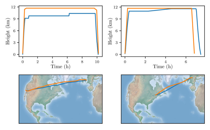
Figure 4: Height profile and skypath of PedricAir (orange) compared to two historic trajectories flown with real aircraft (blue). Left: American Airlines Flight 137 from London Heathrow Airport to Los Angeles International Airport on March 27th 2022. Right: Lufthansa flight 478 from Frankfurt Airport to Montréal Pierre Elliott Trudeau International Airport on March 30th 2022. Flight data courtesy to FlightRadar24.

On $D^{3d}$, we compute flight trajectories using the simplified aircraft PedRicAir. The model is basic, but it ensures realistic horizontal and vertical flight profiles. Thus, the set of relevant TFRs for PedRicAir’s trajectories is similar to the set of relevant TFRs in practice.

Figure 5: Speed triangle. The projected speed $v_{\mathtt{proj}}$ is needed to calculate the top of climb points when climbing along an arc. The descent case behaves symmetrically.

Figure 6: Visualization of a climb maneuver from a level $\ell$ to a higher level $\ell^{\prime}$. The reference/projected arc is $a=(u,v)$ with length $d_{uv}$.

In Fig. 4, we compare the trajectories obtained using PedricAir with those flown by real aircraft in the past.

For our aircraft, we assume a constant speed of Mach $0.7$ which is equivalent to $v=240.1\frac{m}{s}$. Thus, the duration for flying along an arc $a$ with length $d_{a}$, specified in kilometers, at speed $v$ is

$$\mathtt{duration}(a)=10^{3}\frac{d_{a}}{v}\unit{s}.$$ (11)

An optimal cruise level, which we assume to be flight level $181$ at altitude $$11\,300$\unit{m}$, is a flight level at which cruising for a given length yields a minimal fuel consumption. In this section, we denote this flight level by $\ell^{*}$. According to [53] a typical consumption of a commercial aircraft is $0.03{\frac{kg}{km}}$ per seat. If we assume that our aircraft can transport $200$ passengers, this gives us a fuel consumption of $f=6\frac{kg}{km}$, which we assume to be attained when cruising at level $\ell^{*}$. For any flight level $\ell$ and an arc $a$ with length $d_{a}$, specified in kilometers, the cruise consumption of our aircraft along $a$ is given by

$$\mathtt{consumption}(a)=d_{a}\cdot f\cdot 1.01^{|\ell^{*}-\ell|}\unit{kg}.$$ (12)

The typical consumption $f$ specified in [53] refers to the consumption of a commercial aircraft along a whole flight.

Climb and Descent

We fix the climb and descent rate of our aircraft to be $\delta=2.500\unit{\frac{ft}{min}}=12.7\unit{\frac{m}{s}}$ and only allow it to perform step climbs.

Suppose the aircraft is about to climb along the projected arc $a=(u,v)$ from level $\ell$ at $u$ to level $\ell^{\prime}$ at $v$. The length of $a$ is given in meters as $d_{a}$, and we denote the altitude difference between $\ell$ and $\ell^{\prime}$ by $\Delta_{\ell,\ell^{\prime}}$. Since the climb velocity of the aircraft is constant, the climb procedure takes exactly $\mathtt{climb}_{\ell,\ell^{\prime}}:=\frac{\Delta_{\ell,\ell^{\prime}}}{\delta}$ seconds. As shown in Figure 6, we denote the projected speed of the aircraft in meters per second by $v_{\mathtt{proj}}$. Hence, the aircraft has $\frac{d_{a}}{v_{\mathtt{proj}}}$ seconds to climb from $\ell$ to $\ell^{\prime}$ and the climb procedure is only allowed if

$$\mathtt{climb}_{\ell,\ell^{\prime}}\leq\frac{d_{a}}{v_{\mathtt{proj}}}.$$ (13)

Most often, the above inequality is not tight. This explains the step in the step climb procedure: after reaching level $\ell^{\prime}$ along arc $a$, the aircraft continues cruising at this level until $v$ at level $\ell^{\prime}$ is reached. Figure 6 shows an example. The point at which the aircraft stops climbing is called top of climb (TOC). Projected on the surface, $d_{\mathtt{climb}(\ell,\ell^{\prime})}:=v_{\mathtt{proj}}\cdot\mathtt{climb}_{\ell,\ell^{\prime}}$ meters are flown during the climb phase and thus, to reach $v$ at level $\ell^{\prime}$ the aircraft has to cruise for $d_{uv}-d_{\mathtt{climb}(\ell,\ell^{\prime})}$ meters.

The duration of the whole traversal of the arc while climbing is derived in a straightforward way from $v$, $\delta$, and the calculated TOC.

For the consumption, we assume that a climb from $\ell$ to $\ell^{\prime}$ during $d$ meters consumes as much as cruising $d$ meters at level $\lfloor\frac{\mathtt{alt}_{\ell}+\mathtt{alt}_{\ell^{\prime}}}{2}\rfloor$. During descent from $\ell$ to $\ell^{\prime}$, we assume a consumption equal to the consumption while cruising at the source level $\ell$.

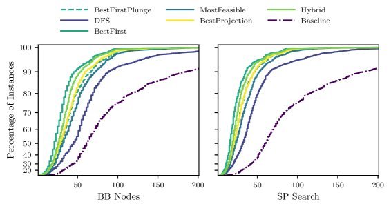
Figure 7: Cumulative distribution plot of solved instances per number of B&B nodes (left) and actual performed shortest path queries (right) for the DFS, best-first search, most-feasible search and best-first search with plunging node selection rules. We truncated the $x$-axis after 200 nodes, at which point 99.9% of all instances are solved using best-first search node selection.

5.3 Experiments

We conducted two experiments to evaluate the performance of the node selection and branching rules described in Section 3 in Algorithm 1. Additionally, we evaluate the overall impact of choosing appropriate node selection and branching rules, by comparing against a baseline configuration. The baseline consists of DFS node selection, which is the standard in SAT solving, together with an uninformed ad-hoc branching rule that simply branches on the first literal in the smallest violated clause (clause). It hence branches on non-graph conflicts.

In the first experiment, we fix SUP branching on graph variables as the branching rule and benchmark different node selection rules against each other. We evaluate the DFS, most-feasible search, best-first search, best-projection search, and the best-first search with plunging node selections rules.

In the second experiment, we fix the best-first search node selection rule and benchmark different branching strategies. We evaluate the MOMS, Strong Branching, CVDS, SUP, DUP, and clause branching rules. We applied MOMS, CVDS, SUP, and DUP on standard conflicts (9) as well as on graph conflicts (10). Strong branching was applied with working limits and only to graph conflicts, as it performed poorly on non-graph conflicts in preliminary experiments. The choice of the fixed branching rule in the first experiment and the fixed node selection rule in the second experiment is motivated by the respective methods’ strong performance in preliminary experiments.

All experiments were run on workstations with a 2 Ghz Intel(R) Xeon(R) Gold 6338 CPU and 120 GB RAM. Algorithm 1 was implemented in C++20 and compiled with gcc 12.20.

5.4 Instances

Our instance set is defined by the subset of all $s,t$-pairs between 466 large international airports [51]. From this set, we exclude 545 $s,t$-pairs that are not flyable in the airway network. For example, landing in Innsbruck, Austria, or overflying the Himalaya are known to be challenging operations in flight planning. Addressing these is beyond the scope of the paper. In total, $216\,145$ $s,t$-pairs remain. The hardness of these instances varies greatly due to the uneven distribution of TFRs across the globe (Fig. 1). Some instances require several hundred B&B nodes to even obtain a feasible solution, whereas others are not affected by TFRs at all. In fact, using the baseline configuration of Algorithm 1 (see Section 5.3), $81.47$% of the instances are solved directly in the root node and $95.43$% are solved in less than 10 nodes. We consider these instances trivial and drop them from further consideration. On the remaining $9869$ instances, we perform our experiments. All results are available in the online appendix [51].

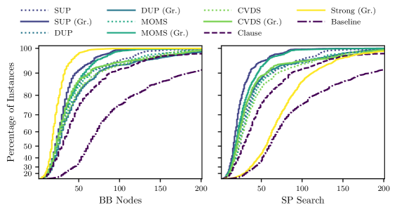
Figure 8: Cumulative distribution plot of solved instances per number of B&B nodes (left) and performed shortest path queries (right) for different branching rules. We truncated the $x$-axis after 200 nodes, at which point 99.9% of all instances are solved using SUP branching on graph conflicts.

5.5 Results

In the following analysis, we filter out any instances that are consistently easy, that is, all instances that are solved in less than $50$ nodes in all studied combinations of branching and node selection rules, including the baseline. We hence consider a data set of 2260 instances.

Using a real aircraft model, the run time of Algorithm 1 is heavily dominated by the shortest path queries. This is because the computation of arc costs (weather and weight-dependent duration and consumption) is a complex task that cannot be precomputed. The most relevant performance measure to evaluate node selection and branching rules is thus the number of calls to the shortest path algorithm and the total number of shortest path iterations, which we measure by the performed arc relaxations. We provide all performance measures, including the number of B&B nodes and run times, in A. Even though we use the simplified PedRicAir aircraft model, the shortest path search still accounts for more than 75% of the run time in all settings.

Figures 7 and 8 depict the cumulative frequency of solved instances over the number of nodes and SP searches for the node selection and branching rule experiment, respectively. Best-first search, which aims at improvements in the dual bound, is the best node selection rule regarding all performance measures. It requires 44.86% fewer B&B nodes, 43.85% fewer SP searches, and 39.29% fewer arc relaxations than DFS, which performs worst. For MIP, using DFS for node selection leads to a higher similarity between subproblems and thus faster subproblem handling. This advantage may even compensate for the larger tree size [54]. Such an advantage cannot be observed for the LCSP: While DFS (${73.56}\mathrm{e}{6}$) requires fewer arc relaxations per shortest path search than best-first search (${79.54}\mathrm{e}{6}$), the effect is only slight and does not translate into a reduction in the total number of arc relaxations. After DFS, the second-worst performance (w.r.t. arc relaxations and SP searches) is achieved by the most-feasible search rule. Both of these rules aim at finding feasible solutions fast.

The remaining node selection rules hybrid search, best-projection search, and best-first search with plunging all aim for a compromise between primal and dual improvements. This sophistication does not pay off: In Fig. 7, we can see that the cumulative frequency of solved instances is for all three rules contained in the band spanned by the most-feasible search and best-first search rules. Moreover, among those three, the best performing rule is hybrid search, which is most similar to best-first search.

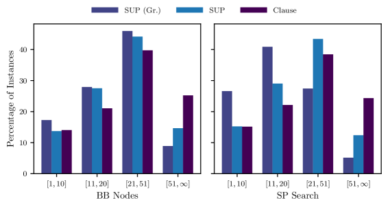
Figure 9: Comparison of the best branching rule SUP on non-graph and graph conflicts using best-first search node selection with the clause branching rule. We plot the percentage of instances solved depending on the number of B&B nodes (left) and on the shortest path queries (right).

The branching rule that attains the least number of B&B nodes is, unsurprisingly, strong branching. This is paid for by computing the most SP queries, making it unsuitable for the realistic flight planning application. Overall, the best-performing branching rule is SUP on graph conflicts, which performs $43$% fewer SP searches and $17.00$% fewer arc relaxations than the baseline branching rule clause.

The second-lowest number of SP searches is attained by MOMS on graph conflicts, which requires $12.94$% more searches than SUP. The lower computational effort of MOMS does not make up for this difference: SUP is still $9.50$% faster, an effect that will be more pronounced for realistic airplane models, and uses $12.46$% fewer arc relaxations. CVDS, applied to graph or non-graph conflicts, outperforms the baseline branching rule clause. It is, however, surpassed by the simpler rules SUP and MOMS that have been abandoned in the SAT community. This may be due to the relatively small B&B trees we observe, which disadvantage learning-based rules. We note that we did not attempt to tune the parameters of CVDS.

SUP performs better than DUP in both the number of SP searches and arc relaxations. This result surprises, given that SUP is essentially a relaxation of DUP. We attribute this to the following reason: SUP performs a single round of unit propagation. This ensures that only unit propagations are counted that can be directly derived from enforcing/forbidding an arc in the current path. In contrast, DUP performs multiple rounds of unit propagation and enforcement in the graph. Enforcing an arc leads to the deletion of all arcs that could be used to bypass it w.r.t the topological sorting on $G_{|T}$. Such arcs may lie in parts of $G_{|T}$ that are far away and never considered in the shortest path search. Their deletion may consequently trigger unit propagations in irrelevant clauses that are not violated by any computed path. In the DUP rule, these unit propagations are counted towards a candidate variable’s score and hence steer the search away from more productive branching decisions.

Proposition 2.3 suggests branching on graph conflicts. Indeed, compared to branching on non-graph conflicts, it reduces the number of SP searches by between $6.51$% (DUP) and $30.11$% (SUP). We illustrate this difference for SUP in Fig. 9.

When branching on graph conflicts, the number of arc relaxations per shortest path search increases by between $16.23$% (MOMS) and $35.25$% (SUP). This behavior can be explained as follows: First, branching on non-graph conflicts produces larger trees, and the size of routing graphs $G_{|T}$ correlates negatively with its depth in the B&B tree. Second, a non-graph conflict (Eq. 9) contains free variables that represent whole subformulae of a TFR. Assigning a truth value to such a subformula then leads to the assignment of multiple graph variables via unit propagation. This consequently leads to more enforcements in the routing graph than if branching were done on graph conflicts. As DUP chooses a branching variable that causes the most unit propagations, the effect is most prominent for this rule. When branching on non-graph conflicts, CVDS ($3.85$%) and DUP ($11.32$%) require fewer arc relaxations in total, even though they produce larger B&B trees. This favors the second explanation.

The least number of arc relaxations is still attained by SUP branching on graph conflicts. Here, the effect of branching on graph conflicts on the number of SP searches outweighs the increased effort for solving the shortest path subproblem.

Combining the SUP branching rule, the best-first search node selection rule and branching on graph conflicts appears to be the best configuration of Algorithm 1. Compared to the baseline of DFS node selection with clause branching, it obtains an overall reduction of $75$% in the number of SP searches.

Finally, we consider the $70$ most difficult instances (see Table 3), that is, instances that require more than 300 B&B nodes for any branching rule. On this instance set, the number of SP searches even decreases by $93$% compared to the baseline. Using the above configuration, Algorithm 1 is clearly fit for commercial application: It performs only $22.52$ SP searches and requires only a run time of $129$s in the geometric mean.

6 Conclusion

We proposed a Branch&Bound (B&B) algorithm for the Logic-Constrained Shortest Path Problem. The algorithm allows for the easy adaptation of techniques from the MIP and SAT communities as branching rules and unit propagation. These techniques, however, require careful reevaluation as conventional wisdom no longer applies in the LCSP setting. The strongest branching rule for the LCSP, SUP, for example, is generally considered inadequate in the SAT community. We applied our algorithm to the flight planning problem with traffic flow restrictions and benchmarked it on large-scale $3$d instances with numerous mandatory traffic flow restrictions. Choosing the right combination of techniques reduces the number of shortest path searches required to solve an instance by up to an order of magnitude on the most complicated Flight Planning instances. The obtained run times make the algorithm clearly fit for commercial application.

Appendix A Computation Results

Table 1: Computation results for all node selection rules. We report the geometric mean and maximum of the number of B&B nodes and SP queries as well as the time spent in total and on SP queries. In all cases apart from the baseline (Baseline), SUP branching on graph conflicts was used.

	Nodes		SP		Time			Arc Relax. ($\times{1}\mathrm{e}{6}$)
Node Selection Rule	Mean	Max	Mean	Max	Total (s)	SP (s)	SP(%)	Total	per SP
DFS	35.73	463	26.98	371	197.40	185.51	93.98	1984.78	73.56
MostFeasible	27.92	333	21.32	255	178.14	169.10	94.93	1782.94	83.65
BestFirst	19.70	261	15.15	201	119.66	113.67	94.99	1204.94	79.54
BestFirstPlunge	28.85	291	21.18	225	164.25	155.07	94.41	1764.73	83.33
Hybrid	23.06	262	17.63	202	140.64	133.56	94.97	1398.18	79.29
Projection	24.87	323	19.02	250	156.64	148.48	94.79	1534.77	80.68
Baseline	62.93	791	60.60	780	396.33	375.58	94.76	3776.24	62.31

Table 2: Computation results for all branching rules. We report the geometric mean and maximum of the number of B&B nodes and SP queries, the time spent in total and on SP queries, and the number of arc relaxations. In all cases apart from the baseline, best-first search node selection was used.

	Nodes		SP		Time			Arc Relax. ($\times{1}\mathrm{e}{6}$)
Branching Rule	Mean	Max	Mean	Max	Total (s)	SP (s)	SP(%)	Total	Per SP
SUP	22.71	499	21.68	308	131.85	125.47	95.16	1274.98	58.81
SUP (Gr.)	19.70	261	15.15	201	120.16	114.06	94.92	1204.94	79.54
DUP	21.91	499	20.72	304	175.07	139.26	79.55	1343.78	64.85
DUP (Gr.)	25.16	449	19.37	358	194.12	148.21	76.35	1495.85	77.24
MOMS	23.20	497	22.13	412	157.76	150.79	95.58	1531.60	69.21
MOMS (Gr.)	20.77	233	17.11	177	139.20	132.78	95.39	1376.45	80.44
CVDS	23.38	499	22.33	362	151.10	144.27	95.48	1438.33	64.40
CVDS (Gr.)	22.09	665	19.81	552	154.95	148.52	95.85	1493.75	75.41
Clause	27.57	663	26.61	537	158.69	150.88	95.08	1451.69	54.56
Strong (Gr.)	15.18	129	49.28	557	305.75	286.53	93.71	2481.50	50.36
Baseline	62.93	791	60.60	780	396.33	375.58	94.76	3776.24	62.31

Table 3: Computation results for the 70 most difficult instances. We include all instances that require more than 300 B&B Nodes for at least one configuration, including the baseline. We report the geometric mean and maximum of the number of B&B nodes and SP queries, the time spent in total and on SP queries, and the number of arc relaxations. In all cases apart from the baseline, best-first search node selection was used.

	Nodes		SP		Time			Arc Relax. ($\times{1}\mathrm{e}{6}$)
Branching Rule	Mean	Max	Mean	Max	Total (s)	SP (s)	SP(%)	Total	Per SP
SUP	45.23	499	41.86	308	151.43	138.24	91.29	1230.78	29.40
SUP (Gr.)	30.83	261	22.52	201	137.92	129.29	93.75	1344.62	59.71
DUP	43.05	499	39.50	304	261.05	147.24	56.40	1193.25	30.21
DUP (Gr.)	42.64	449	31.00	358	242.72	172.80	71.20	1499.56	48.37
MOMS	50.08	497	45.26	412	192.45	175.68	91.29	1522.01	33.63
MOMS (Gr.)	33.88	233	27.26	174	161.93	152.18	93.97	1485.67	54.49
CVDS	57.49	499	52.79	362	182.76	162.97	89.18	1325.06	25.10
CVDS (Gr.)	41.03	665	35.35	552	186.07	175.72	94.44	1466.35	41.48
Clause	85.80	663	79.56	537	267.12	238.16	89.16	1599.08	20.10
Strong (Gr.)	19.81	129	58.71	557	308.93	286.44	92.72	2051.72	34.95
Baseline	349.29	791	323.38	780	1349.53	1201.00	88.99	9898.61	30.61

References

- Blanco et al. [2016a] M. Blanco, R. Borndörfer, N.-D. Hoang, A. Kaier, T. Schlechte, S. Schlobach, The Shortest Path Problem with Crossing Costs, Technical Report 16-70, Zuse Institute Berlin, Takustr. 7, 14195 Berlin, 2016a. URL: urn:nbn:de:0297-zib-61240.
- Blanco et al. [2016b] M. Blanco, R. Borndörfer, N.-D. Hoang, A. Kaier, A. Schienle, T. Schlechte, S. Schlobach, Solving time dependent shortest path problems on airway networks using super-optimal wind, in: M. Goerigk, R. F. Werneck (Eds.), 16th Workshop on Algorithmic Approaches for Transportation Modelling, Optimization, and Systems (ATMOS 2016), volume 54 of Open Access Series in Informatics (OASIcs), Schloss Dagstuhl – Leibniz-Zentrum für Informatik, Dagstuhl, Germany, 2016b, pp. 12:1–12:15. doi:10.4230/OASIcs.ATMOS.2016.12.
- Blanco et al. [2017] M. Blanco, R. Borndörfer, N. D. Hoàng, A. Kaier, P. Maristany de las Casas, T. Schlechte, S. Schlobach, Cost projection methods for the shortest path problem with crossing costs, in: G. D’Angelo, T. Dollevoet (Eds.), 17th Workshop on Algorithmic Approaches for Transportation Modelling, Optimization, and Systems (ATMOS 2017), volume 59 of OpenAccess Series in Informatics (OASIcs), Schloss Dagstuhl–Leibniz-Zentrum fuer Informatik, Dagstuhl, Germany, 2017, pp. 15:1–15:14. doi:10.4230/OASIcs.ATMOS.2017.15.
- Knudsen et al. [2017] A. N. Knudsen, M. Chiarandini, K. S. Larsen, Constraint handling in flight planning, in: J. C. Beck (Ed.), Principles and Practice of Constraint Programming, Springer International Publishing, Cham, 2017, pp. 354–369. doi:10.1007/978-3-319-66158-2_23.
- Knudsen et al. [2018] A. N. Knudsen, M. Chiarandini, K. S. Larsen, Heuristic variants of search for 3d flight planning, in: W.-J. van Hoeve (Ed.), Integration of Constraint Programming, Artificial Intelligence, and Operations Research, Springer International Publishing, Cham, 2018, pp. 361–376. doi:10.1007/978-3-319-93031-2_26.
- Schienle et al. [2019] A. Schienle, P. Maristany de las Casas, M. Blanco, A Priori Search Space Pruning in the Flight Planning Problem, in: V. Cacchiani, A. Marchetti-Spaccamela (Eds.), 19th Symposium on Algorithmic Approaches for Transportation Modelling, Optimization, and Systems (ATMOS 2019), volume 75 of Open Access Series in Informatics (OASIcs), Schloss Dagstuhl – Leibniz-Zentrum für Informatik, Dagstuhl, Germany, 2019, pp. 8:1–8:14. doi:10.4230/OASIcs.ATMOS.2019.8.
- Kühner [2020] A. Kühner, Shortest Paths with Boolean Constraints, Master’s thesis, Freie Universität Berlin, Department of Mathematics, 2020.
- Blanco et al. [2022] M. Blanco, R. Borndörfer, P. Maristany de las Casas, An A* algorithm for flight planning based on idealized vertical profiles, in: M. D’Emidio, N. Lindner (Eds.), 22nd Symposium on Algorithmic Approaches for Transportation Modelling, Optimization, and Systems (ATMOS 2022), volume 106 of Open Access Series in Informatics (OASIcs), Schloss Dagstuhl – Leibniz-Zentrum für Informatik, Dagstuhl, Germany, 2022, pp. 1:1–1:15. doi:10.4230/OASIcs.ATMOS.2022.1.
- Ramalingam and Reps [1996a] G. Ramalingam, T. Reps, An incremental algorithm for a generalization of the shortest-path problem, Journal of Algorithms 21 (1996a) 267–305. URL: https://www.sciencedirect.com/science/article/pii/S0196677496900462. doi:10.1006/jagm.1996.0046.
- Ramalingam and Reps [1996b] G. Ramalingam, T. Reps, On the computational complexity of dynamic graph problems, Theoretical Computer Science 158 (1996b) 233–277. URL: https://www.sciencedirect.com/science/article/pii/0304397595000798. doi:10.1016/0304-3975(95)00079-8.
- Frigioni et al. [2000] D. Frigioni, A. Marchetti-Spaccamela, U. Nanni, Fully dynamic algorithms for maintaining shortest paths trees, Journal of Algorithms 34 (2000) 251–281. URL: https://www.sciencedirect.com/science/article/pii/S0196677499910489. doi:10.1006/jagm.1999.1048.
- Narvaez et al. [2000] P. Narvaez, K.-Y. Siu, H.-Y. Tzeng, New dynamic algorithms for shortest path tree computation, IEEE/ACM Transactions on Networking 8 (2000) 734–746. doi:10.1109/90.893870.
- Koenig et al. [2004] S. Koenig, M. Likhachev, D. Furcy, Lifelong planning , Artificial Intelligence 155 (2004) 93–146. URL: https://www.sciencedirect.com/science/article/pii/S000437020300225X. doi:10.1016/j.artint.2003.12.001.
- Bauer and Wagner [2009] R. Bauer, D. Wagner, Batch dynamic single-source shortest-path algorithms: An experimental study, in: J. Vahrenhold (Ed.), Experimental Algorithms, Springer Berlin Heidelberg, Berlin, Heidelberg, 2009, pp. 51–62. doi:10.1007/978-3-642-02011-7_7.
- D’Andrea et al. [2014] A. D’Andrea, M. D’Emidio, D. Frigioni, S. Leucci, G. Proietti, Experimental evaluation of dynamic shortest path tree algorithms on homogeneous batches, in: J. Gudmundsson, J. Katajainen (Eds.), Experimental Algorithms, Springer International Publishing, Cham, 2014, pp. 283–294. doi:10.1007/978-3-319-07959-2_24.
- Aloul et al. [2006] F. A. Aloul, B. A. Rawi, M. Aboelaze, Identifying the shortest path in large networks using boolean satisfiability, in: 2006 3rd International Conference on Electrical and Electronics Engineering, 2006, pp. 1–4. doi:10.1109/ICEEE.2006.251924.
- Nishino et al. [2015] M. Nishino, N. Yasuda, S.-i. Minato, M. Nagata, BDD-constrained search: A unified approach to constrained shortest path problems, Proceedings of the AAAI Conference on Artificial Intelligence 29 (2015). doi:10.1609/aaai.v29i1.9373.
- Bryant [1986] R. E. Bryant, Graph-based algorithms for boolean function manipulation, IEEE Transactions on Computers 100 (1986) 677–691. doi:10.1109/TC.1986.1676819.
- Barrett et al. [2000] C. Barrett, R. Jacob, M. Marathe, Formal-language-constrained path problems, SIAM J. Comput. 30 (2000) 809–837. doi:10.1137/S0097539798337716.
- Euler et al. [2024] R. Euler, N. Lindner, R. Borndörfer, Price optimal routing in public transportation, EURO Journal on Transportation and Logistics 13 (2024) 100128. doi:https://doi.org/10.1016/j.ejtl.2024.100128.
- Parmentier [2019] A. Parmentier, Algorithms for non-linear and stochastic resource constrained shortest path, Mathematical Methods of Operations Research 89 (2019) 281–317. URL: https://doi.org/10.1007/s00186-018-0649-x. doi:10.1007/s00186-018-0649-x.
- Gabow et al. [1976] H. N. Gabow, S. N. Maheshwari, L. J. Osterweil, On two problems in the generation of program test paths, IEEE Transactions on Software Engineering SE-2 (1976) 227–231. doi:10.1109/TSE.1976.233819.
- Tseitin [1983] G. S. Tseitin, On the complexity of derivation in propositional calculus, in: J. H. Siekmann, G. Wrightson (Eds.), Automation of Reasoning: 2: Classical Papers on Computational Logic 1967–1970, Springer Berlin Heidelberg, Berlin, Heidelberg, 1983, pp. 466–483. doi:10.1007/978-3-642-81955-1_28.
- Biere and Fröhlich [2015] A. Biere, A. Fröhlich, Evaluating cdcl variable scoring schemes, in: M. Heule, S. Weaver (Eds.), Theory and Applications of Satisfiability Testing – SAT 2015, Springer International Publishing, Cham, 2015, pp. 405–422. doi:10.1007/978-3-319-24318-4\_29.
- Davis et al. [1962] M. Davis, G. Logemann, D. Loveland, A machine program for theorem-proving, Communications of the ACM 5 (1962) 394–397. doi:10.1145/368273.368557.
- Marques Silva and Sakallah [1996] J. Marques Silva, K. Sakallah, Grasp-a new search algorithm for satisfiability, in: Proceedings of International Conference on Computer Aided Design, 1996, pp. 220–227. doi:10.1109/ICCAD.1996.569607.
- Moskewicz et al. [2001] M. W. Moskewicz, C. F. Madigan, Y. Zhao, L. Zhang, S. Malik, Chaff: engineering an efficient sat solver, in: Proceedings of the 38th Annual Design Automation Conference, DAC ’01, Association for Computing Machinery, New York, NY, USA, 2001, p. 530–535. doi:10.1145/378239.379017.
- Ryan [2004] L. Ryan, Efficient algorithms for clause-learning SAT solvers, Master’s thesis, Simon Fraser University, 2004.
- Biere et al. [2021] A. Biere, M. Heule, H. van Maaren, T. Walsh (Eds.), Handbook of Satisfiability - Second Edition, volume 336 of Frontiers in Artificial Intelligence and Applications, IOS Press, 2021. doi:10.3233/FAIA336.
- Loveland [1970] D. W. Loveland, A linear format for resolution, in: M. Laudet, D. Lacombe, L. Nolin, M. Schützenberger (Eds.), Symposium on Automatic Demonstration, Springer Berlin Heidelberg, Berlin, Heidelberg, 1970, pp. 147–162. doi:10.1007/BFb0060630.
- Kahn [1962] A. B. Kahn, Topological sorting of large networks, Commun. ACM 5 (1962) 558–562. doi:10.1145/368996.369025.
- Eén and Sörensson [2003] N. Eén, N. Sörensson, An extensible sat-solver, in: International conference on theory and applications of satisfiability testing, Springer, 2003, pp. 502–518. doi:10.1007/978-3-540-24605-3_37.
- Marques-Silva et al. [2021] J. Marques-Silva, I. Lynce, S. Malik, Conflict-driven clause learning, in: [29], 2021, pp. 133 –182. doi:10.3233/FAIA336.
- Achterberg [2007] T. Achterberg, Constraint Integer Programming, Ph.D. thesis, Technische Universität Berlin, 2007.
- Dakin [1965] R. J. Dakin, A tree-search algorithm for mixed integer programming problems, The Computer Journal 8 (1965) 250–255. doi:10.1093/comjnl/8.3.250.
- Linderoth and Savelsbergh [1999] J. T. Linderoth, M. W. P. Savelsbergh, A computational study of search strategies for mixed integer programming, INFORMS Journal on Computing 11 (1999) 173–187. doi:10.1287/ijoc.11.2.173.
- Wojtaszek and Chinneck [2010] D. T. Wojtaszek, J. W. Chinneck, Faster mip solutions via new node selection rules, Computers & Operations Research 37 (2010) 1544–1556. URL: https://www.sciencedirect.com/science/article/pii/S0305054809003074. doi:10.1016/j.cor.2009.11.011.
- Hajian and Mitra [1995] M. Hajian, G. Mitra, Design and testing of an integrated branch and bound algorithm for piecewise linear and discrete programming problems, Technical Report, Technical Report TR/01/95, Brunel, the University of West London, London, 1995.
- Hirst [1969] J. Hirst, Features required in branch and bound algorithms for (0-1) mixed integer linear programming, Privately circulated manuscript (1969).
- Benichou et al. [1971] M. Benichou, J. M. Gauthier, P. Girodet, G. Hentges, G. Ribiere, O. Vincent, Experiments in mixed-integer linear programming, Mathematical Programming 1 (1971) 76–94. doi:10.1007/BF01584074.
- Applegate et al. [1995] D. Applegate, R. Bixby, V. Chvátal, W. Cook, Finding cuts in the tsp (a preliminary report), 1995.
- Gamrath and Schubert [2018] G. Gamrath, C. Schubert, Measuring the impact of branching rules for mixed-integer programming, in: N. Kliewer, J. F. Ehmke, R. Borndörfer (Eds.), Operations Research Proceedings 2017, Springer International Publishing, Cham, 2018, pp. 165–170. doi:10.1007/978-3-319-89920-6_23.
- Bolusani et al. [2024] S. Bolusani, M. Besançon, K. Bestuzheva, A. Chmiela, J. Dionísio, T. Donkiewicz, J. van Doornmalen, L. Eifler, M. Ghannam, A. Gleixner, et al., The scip optimization suite 9.0, arXiv preprint (2024). arXiv:arXiv:2402.17702.
- Achterberg and Berthold [2009] T. Achterberg, T. Berthold, Hybrid branching, in: W.-J. van Hoeve, J. N. Hooker (Eds.), Integration of AI and OR Techniques in Constraint Programming for Combinatorial Optimization Problems, Springer Berlin Heidelberg, Berlin, Heidelberg, 2009, pp. 309–311. doi:10.1007/978-3-642-01929-6_23.
- Dey et al. [2024] S. S. Dey, Y. Dubey, M. Molinaro, P. Shah, A theoretical and computational analysis of full strong-branching, Mathematical Programming 205 (2024) 303–336. doi:10.1007/s10107-023-01977-x.
- Mexi et al. [2024] G. Mexi, S. Shamsi, M. Besançon, P. Le Bodic, Probabilistic lookahead strong branching via a stochastic abstract branching model, in: B. Dilkina (Ed.), Integration of Constraint Programming, Artificial Intelligence, and Operations Research, Springer Nature Switzerland, Cham, 2024, pp. 56–73. doi:10.1007/978-3-031-60599-4_4.
- Lagoudakis and Littman [2001] M. G. Lagoudakis, M. L. Littman, Learning to select branching rules in the DPLL procedure for satisfiability, Electronic Notes in Discrete Mathematics 9 (2001) 344–359. doi:10.1016/S1571-0653(04)00332-4, lICS 2001 Workshop on Theory and Applications of Satisfiability Testing (SAT 2001).
- Crawford and Auton [1996] J. M. Crawford, L. D. Auton, Experimental results on the crossover point in random 3-sat, Artificial Intelligence 81 (1996) 31–57. doi:10.1016/0004-3702(95)00046-1, frontiers in Problem Solving: Phase Transitions and Complexity.
- Li and Anbulagan [1997] C. M. Li, A. Anbulagan, Heuristics based on unit propagation for satisfiability problems, in: Proceedings of the 15th International Joint Conference on Artifical Intelligence - Volume 1, IJCAI’97, Morgan Kaufmann Publishers Inc., San Francisco, CA, USA, 1997, p. 366–371.
- Hart et al. [1968] P. E. Hart, N. J. Nilsson, B. Raphael, A formal basis for the heuristic determination of minimum cost paths, IEEE Transactions on Systems Science and Cybernetics 4 (1968) 100–107. doi:10.1109/TSSC.1968.300136.
- Euler and Maristany de las Casas [2024] R. Euler, P. Maristany de las Casas, Supplementary material, Zenodo repository, 2024. doi:10.5281/zenodo.14391762.
- Eurocontrol [2024] Eurocontrol, Rad general description, 2024. URL: https://www.nm.eurocontrol.int/RAD/, [accessed 21.11.2024].
- Kühn [2024] M. Kühn, Fuel consumption of the 50 most used passenger aircraft, 2024. doi:10.7910/DVN/4CYNKA.
- Achterberg et al. [2005] T. Achterberg, T. Koch, A. Martin, Branching rules revisited, Operations Research Letters 33 (2005) 42–54. URL: https://www.sciencedirect.com/science/article/pii/S0167637704000501. doi:10.1016/j.orl.2004.04.002.