Chaotic dynamics and fractal geometry
in ring lattice systems of non-chaotic Rulkov neurons

Abstract

This paper investigates the complex dynamics and fractal attractors that emerge from 60-dimensional ring lattice systems of electrically coupled non-chaotic Rulkov neurons. Although networks of chaotic Rulkov neurons are well-studied, systems of non-chaotic Rulkov neurons have not been extensively explored due to the piecewise complexity of the non-chaotic Rulkov map. We find rich dynamics emerge from the electrical coupling of regular spiking Rulkov neurons, including chaotic spiking, chaotic bursting, and complete chaos. We also discover general trends in the maximal Lyapunov exponent among different ring lattice systems as the electrical coupling strength between neurons is varied. By means of the Kaplan-Yorke conjecture, we also examine the fractal geometry of the chaotic attractors of the ring systems and find various correlations and differences between the fractal dimensions of the attractors and the chaotic dynamics on them.

I Introduction

Biological neurons are well-known to exhibit a wide variety of interesting dynamic behaviors, including non-chaotic and chaotic spiking and bursting [1]. Since the pioneering work of Hodgkin and Huxley [2], many continuous-time neuron models have been developed in an attempt to model the complex behavior of biological neurons [3, 4, 5, 6]. In order to capture the dynamics of neurons with fast bursts of spikes on top of slow oscillations, many of these models are slow-fast dynamical systems [7, 8, 9, 10, 11, 12]. However, these systems of nonlinear differential equations are often unwieldy to work with, posing a significant computational obstacle in modeling the behavior of many neuron systems [13]. As a result, some discrete-time neuron models have been proposed, such as Rulkov’s simple two-dimensional slow-fast models [14, 15].

These models, often called the chaotic and non-chaotic Rulkov models [16], are capable of modeling both chaotic and non-chaotic spiking and bursting behaviors, and they are computationally efficient, allowing for the study of neuron systems with a complex architecture. The chaotic Rulkov model has been well-studied in the literature [16, 17, 18, 19, 20, 21], but in this paper, we will focus on the non-chaotic Rulkov model, which also produces rich and interesting dynamics. As expected, the most direct application of the (non-chaotic) Rulkov map is in modeling neuronal dynamics [14], but it has also shown application in stability analysis [22], control of chaos [23], symbolic analysis [24], machine learning [25], information patterns [26], and digital watermarking [27]. Therefore, it is a worthwhile system to study purely for its dynamical and geometrical properties.

The non-chaotic Rulkov map is defined by the following iteration function :

$$\begin{pmatrix}x_{k+1}\\ y_{k+1}\end{pmatrix}=\begin{pmatrix}f(x_{k},y_{k};\alpha)\\ y_{k}-\mu(x_{k}-\sigma)\end{pmatrix},$$ (1)

where $f$ is the piecewise function

$$f(x,y;\alpha)=\begin{cases}\alpha/(1-x)+y,&x\leq 0\\ \alpha+y,&0<x<\alpha+y\\ -1,&x\geq\alpha+y\end{cases}.$$ (2)

Here, $\mathbf{x}_{k}=(x_{k},y_{k})$ is the state of the system at time step $t=k$, $x$ is the fast variable representing the voltage of the neuron, $y$ is the slow variable, and $\alpha$, $\sigma$, and $\mu$ are parameters. To make $y$ a slow variable, we need $0<\mu\ll 1$, so we choose the standard value of $\mu=0.001$.

In experiments, biologists can alter the behavior of biological neurons by injecting the cell with a direct electrical current through an electrode [14]. Modeling an injection of current from a DC voltage source requires a slight modification of the Rulkov iteration equation in Eq. 1:

$$\begin{pmatrix}x_{k+1}\\ y_{k+1}\end{pmatrix}=\begin{pmatrix}f(x_{k},y_{k}+\beta_{k};\alpha)\\ y_{k}-\mu(x_{k}-\sigma_{k})\end{pmatrix},$$ (3)

where the parameters $\beta_{k}$ and $\sigma_{k}$ model a time-varying injected current.

In this paper, we are interested in lattice systems of coupled non-chaotic Rulkov neurons. So far, networks of coupled chaotic Rulkov neurons have received much attention, especially regarding the synchronization of chaotic Rulkov neuron networks. For example, existing studies include two chaotic Rulkov neurons coupled with chemical synapses [29], two chaotic Rulkov neurons with a chemical synaptic and inner linking coupling [30], the complete synchronization of an electrically coupled chaotic Rulkov neuron network [31], and synchronization in a master-slave network structure of chaotic Rulkov neurons [32]. However, coupled systems of non-chaotic Rulkov neurons have not nearly received as much attention due to the complexity of the piecewise function $f$ present in the non-chaotic Rulkov map (Eq. 2). Here, we are interested in lattice structures of non-chaotic Rulkov neurons that are electrically coupled with a flow of current. Specifically, say we have some coupled Rulkov neurons with states $\mathbf{x}_{i}$, where $i$ denotes the neuron index. Then, mirroring Eq. 3, we define the iteration function of the $i$th coupled neuron to be

$$\begin{pmatrix}x_{i,k+1}\\ y_{i,k+1}\end{pmatrix}=\begin{pmatrix}f(x_{i,k},y_{i,k}+\mathfrak{C}_{i,x}(k);\alpha_{i})\\[2.00749pt] y_{i,k}-\mu x_{i,k}+\mu[\sigma_{i}+\mathfrak{C}_{i,y}(k)]\end{pmatrix},$$ (4)

where $\mathbf{x}_{i,k}$ is the state of the neuron $\mathbf{x}_{i}$ at the time step $k$. The coupling parameters $\mathfrak{C}_{i,x}(t)$ and $\mathfrak{C}_{i,y}(t)$ depend on the structural arrangement of the system’s neurons in physical space, as well as the electrical coupling strength (or coupling conductance) $g^{e}$ between the neurons.

In electrically coupled neuron systems, the difference in the voltages, or fast variables, of two adjacent neurons is what results in a flow of current between them. For this reason, we model the electrical coupling parameters $\mathfrak{C}_{i,x}(t)$ and $\mathfrak{C}_{i,y}(t)$ to be proportional to the difference between the voltage of a given neuron $\mathbf{x}_{i}$ and the voltages of its adjacent neurons $\mathbf{x}_{j}$. Specifically, the electrical coupling parameters of the neuron $\mathbf{x}_{i}$ are defined to be

$$\mathfrak{C}_{i,x}(t)=\frac{\beta^{c}_{i}}{|\mathcal{N}_{i}|}\sum_{j\in\mathcal{N}_{i}}g^{e}_{ji}(x_{j,t}-x_{i,t}),$$ (5)

$$\mathfrak{C}_{i,y}(t)=\frac{\sigma^{c}_{i}}{|\mathcal{N}_{i}|}\sum_{j\in\mathcal{N}_{i}}g^{e}_{ji}(x_{j,t}-x_{i,t}),$$ (6)

where $\mathcal{N}_{i}$ is the set of neurons that are adjacent to $\mathbf{x}_{i}$ and $g^{e}_{ji}$ is the electrical coupling strength from $\mathbf{x}_{j}$ to $\mathbf{x}_{i}$ [16].

In this paper, we investigate a ring lattice structure of neurons inspired by Refs. [33, 34]. Specifically, we are interested in a ring of $\zeta$ electrically coupled non-chaotic Rulkov neurons $\mathbf{x}_{0},\mathbf{x}_{1},\ldots,\mathbf{x}_{\zeta-1}$, each having a flow of current with its neighbor. Osipov et al. [35] qualitatively describe the dynamics of a similar Rulkov ring lattice system, noting the emergence of complex dynamics from Rulkov neurons in the non-chaotic spiking regime. In this paper, we build on this work with a quantitative analysis of the chaotic dynamics of three ring lattice systems, each with different individual neuron behaviors. We find that the piecewise function $f$ present in the iteration function of each neuron in the ring yields an impressively complex Jacobian matrix. Using this, we explore the dynamics of these systems in greater generality over a wide range of electrical coupling strength values through a computation of the systems’ maximal Lyapunov exponents. We also analyze the fractal geometry of the high-dimensional chaotic attractors of the systems and how they change as the electrical coupling strength varies. Finally, we explore the links between the dynamics on the attractors and the attractors’ fractalization.

This paper is organized as follows. In Sec. II, we describe the model and the three systems of interest, then we present our qualitative and quantitative analysis of their complex dynamics. In Sec. III, we overview the Kaplan-Yorke conjecture and use it to approximate the fractal dimensions of the systems’ attractors in 60-dimensional state space. Finally, in Sec. IV, we summarize our results and give implications and suggestions for future research.

Figure 1: Visualization of a ring of $\zeta=30$ Rulkov 1 neurons

II The model and dynamics

The model we investigate in this paper is a ring lattice of $\zeta$ electrically coupled non-chaotic Rulkov neurons. This lattice structure is visualized in Fig. 1 for $\zeta=30$, where neurons are represented by blue points and the electric coupling connections are shown in gold.

To calculate the coupling parameters for each of these neurons, let $\beta^{c}_{i}=\sigma^{c}_{i}=1$ for simplicity. We will also assume that all couplings are equivalent and symmetric: $g^{e}=g^{e}_{ji}$ for all $i\neq j$. Because of the circular nature of this lattice system, we can write $\mathcal{N}_{i}$ as

$$\mathcal{N}_{i}=\{\mathbf{x}_{(i-1)\bmod\zeta},\mathbf{x}_{(i+1)\bmod\zeta}\},$$ (7)

which accounts for the fact that $\mathcal{N}_{0}=\{\mathbf{x}_{\zeta-1},\mathbf{x}_{1}\}$ and $\mathcal{N}_{\zeta-1}=\{\mathbf{x}_{\zeta-2},\mathbf{x}_{0}\}$. Then, from Eqs. 5 and 6, the coupling parameters of this ring system are

$$\begin{split}\mathfrak{C}_{i}&=\mathfrak{C}_{i,x}=\mathfrak{C}_{i,y}\\ &=\frac{g^{e}}{2}[(x_{(i-1)\bmod\zeta}-x_{i})+(x_{(i+1)\bmod\zeta}-x_{i})]\\ &=\frac{g^{e}}{2}[x_{(i-1)\bmod\zeta}+x_{(i+1)\bmod\zeta}-2x_{i}].\end{split}$$ (8)

The state vector of this entire ring system with all $\zeta$ neurons can be written as

$$\mathbf{X}=\begin{pmatrix}X^{[1]}\\ X^{[2]}\\ X^{[3]}\\ X^{[4]}\\ \vdots\\[3.01125pt] X^{[2\zeta-1]}\\ X^{[2\zeta]}\end{pmatrix}=\begin{pmatrix}x_{0}\\ y_{0}\\ x_{1}\\ y_{1}\\ \vdots\\ x_{\zeta-1}\\ y_{\zeta-1}\end{pmatrix},$$ (9)

where $X^{[p]}$ is the $p$th dimension of the state vector $\mathbf{X}$. The state space of this ring lattice system is $2\zeta$-dimensional since we have one slow variable and one fast variable for each of the $\zeta$ neurons in the ring. Plugging the coupling parameters (Eq. 8) into the general iteration function for coupled Rulkov maps (Eq. 4) for each neuron in the ring yields the $2\zeta$-dimensional iteration function for the system:

$$\begin{gathered}\mathbf{F}(\mathbf{X})=\begin{pmatrix}F^{[1]}(x_{0},y_{0},x_{1},y_{1},\ldots,x_{\zeta-1},y_{\zeta-1})\\[4.015pt] F^{[2]}(x_{0},y_{0},x_{1},y_{1},\ldots,x_{\zeta-1},y_{\zeta-1})\\[4.015pt] F^{[3]}(x_{0},y_{0},x_{1},y_{1},\ldots,x_{\zeta-1},y_{\zeta-1})\\[4.015pt] F^{[4]}(x_{0},y_{0},x_{1},y_{1},\ldots,x_{\zeta-1},y_{\zeta-1})\\[4.015pt] \vdots\\[4.015pt] F^{[2\zeta-1]}(x_{0},y_{0},x_{1},y_{1},\ldots,x_{\zeta-1},y_{\zeta-1})\\[4.015pt] F^{[2\zeta]}(x_{0},y_{0},x_{1},y_{1},\ldots,x_{\zeta-1},y_{\zeta-1})\end{pmatrix}\\[7.11317pt] =\begin{pmatrix}f\Big{(}x_{0},y_{0}+\frac{g^{e}}{2}(x_{\zeta-1}+x_{1}-2x_{0});\alpha_{0}\Big{)}\\[4.015pt] y_{0}-\mu x_{0}+\mu\Big{[}\sigma_{0}+\frac{g^{e}}{2}(x_{\zeta-1}+x_{1}-2x_{0})\Big{]}\\[4.015pt] f\Big{(}x_{1},y_{1}+\frac{g^{e}}{2}(x_{0}+x_{2}-2x_{1});\alpha_{1}\Big{)}\\[4.015pt] y_{1}-\mu x_{1}+\mu\Big{[}\sigma_{1}+\frac{g^{e}}{2}(x_{0}+x_{2}-2x_{1})\Big{]}\\[4.015pt] \vdots\\[4.015pt] f\Big{(}x_{\zeta-1},y_{\zeta-1}+\frac{g^{e}}{2}(x_{\zeta-2}+x_{0}-2x_{\zeta-1});\alpha_{\zeta-1}\Big{)}\\[4.015pt] y_{\zeta-1}-\mu x_{\zeta-1}+\mu\Big{[}\sigma_{\zeta-1}+(x_{\zeta-2}+x_{0}-2x_{\zeta-1})\Big{]}\end{pmatrix}.\vskip 7.11317pt\end{gathered}$$ (10)

We perform our computational analysis on systems with the architecture displayed in Fig. 1: rings of $\zeta=30$ Rulkov neurons. Because each of these neurons has one slow and one fast variable (see Eq. 9), the state spaces of these systems are 60-dimensional. We present the results from our analysis of the dynamics that emerge from three different systems, where

1. different neurons have different $x_{i,0}$ values but the same $y_{i,0}$, $\sigma_{i}$, and $\alpha_{i}$ values,

2. different neurons have different $x_{i,0}$ and $\sigma_{i}$ values but the same $y_{i,0}$ and $\alpha_{i}$ values,

3. and different neurons have different $x_{i,0}$, $\sigma_{i}$, and $\alpha_{i}$ values but the same $y_{i,0}$ values.

We do not consider the case where different neurons have with different $y_{i,0}$ values because different evolutions of the slow variable are accounted for by different values of $\sigma_{i}$ [14].

In Appx. A, we detail a sketch of the derivation of the Jacobian matrix of these systems (Eq. 16). Given some initial state $\mathbf{X}_{0}$, we generate an orbit $O(\mathbf{X}_{0})$ and calculate the Jacobian matrix of the system $J(\mathbf{X})$ at each $\mathbf{X}\in O(\mathbf{X}_{0})$. We then use the QR factorization method detailed in Refs. [36, 37, 38, 39] to compute the 60 Lyapunov exponents of the orbit. We use the maximal Lyapunov exponent to gauge chaotic dynamics in this section, and we use the entire Lyapunov spectrum for our analysis in Sec. III.

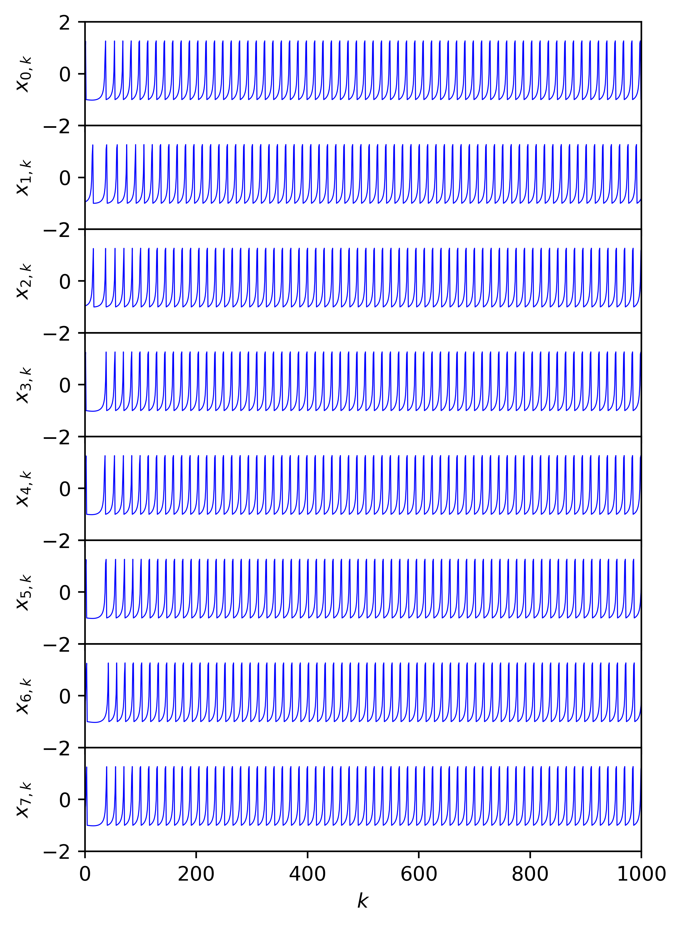
(a) $g^{e}=0$, $\lambda_{1}\approx-0.0938$

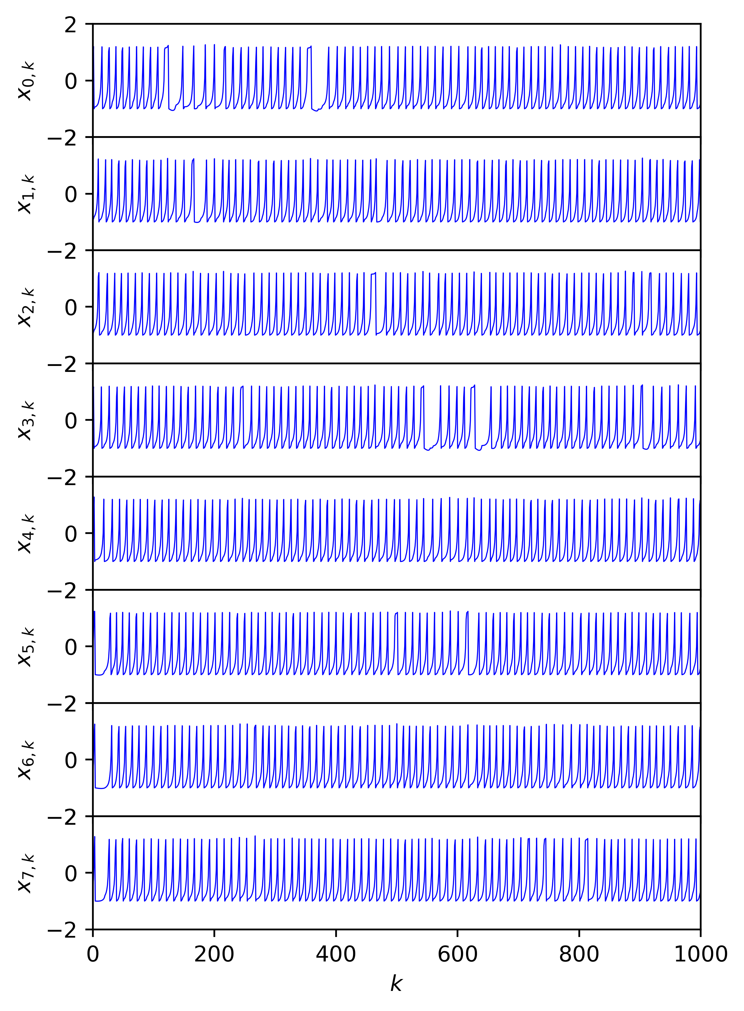
(b) $g^{e}=0.05$, $\lambda_{1}\approx 0.0491$

(c) $g^{e}=0.25$, $\lambda_{1}\approx 0.0595$

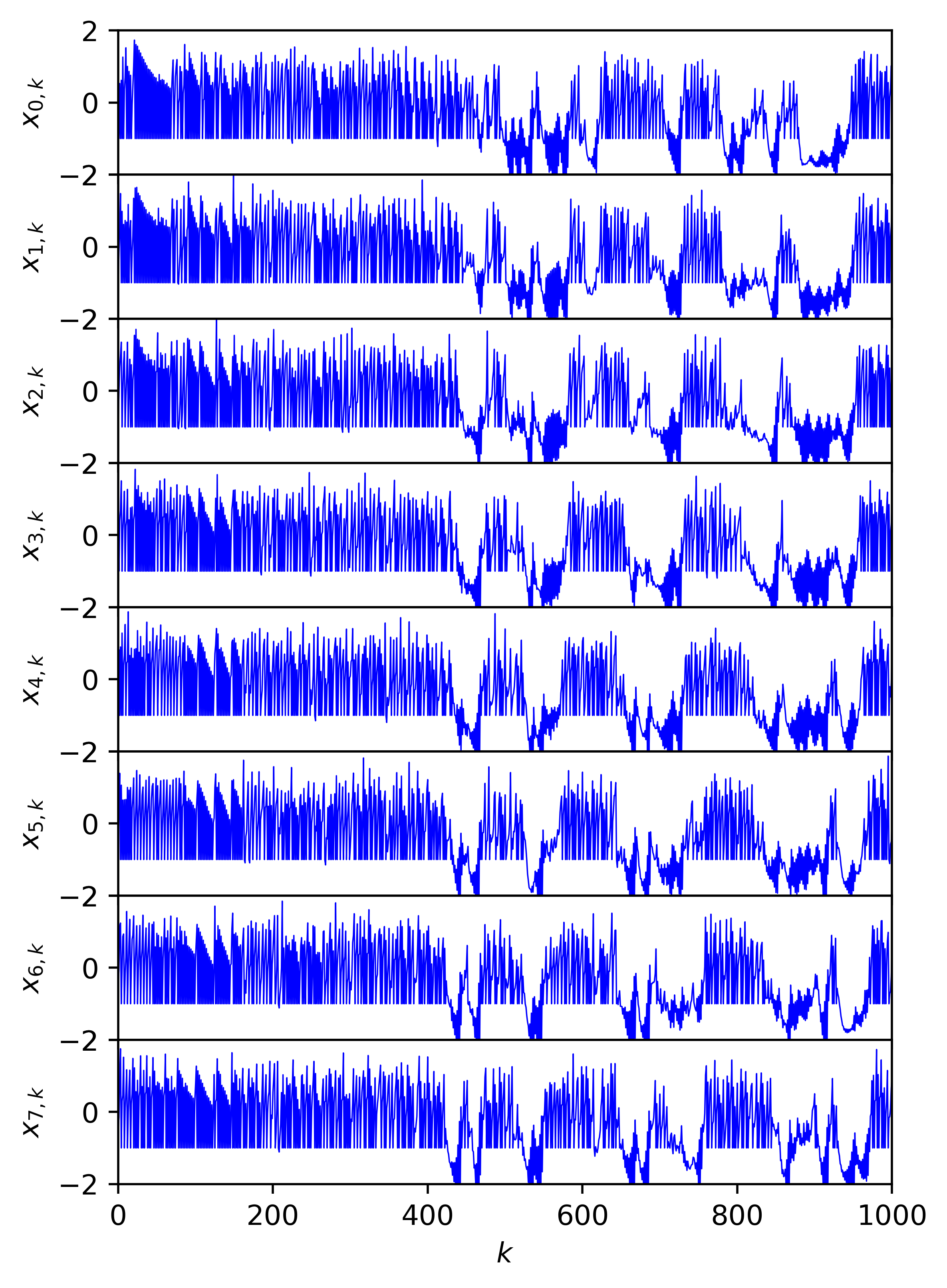
(d) $g^{e}=1$, $\lambda_{1}\approx 0.1694$

Figure 2: Graphs of the fast variable orbits of the first eight neurons in the first ring lattice system, with $x_{i,0}\in(-1,1)$, $y_{i,0}=-3.25$, $\sigma_{i}=-0.5$, and $\alpha_{i}=4.5$

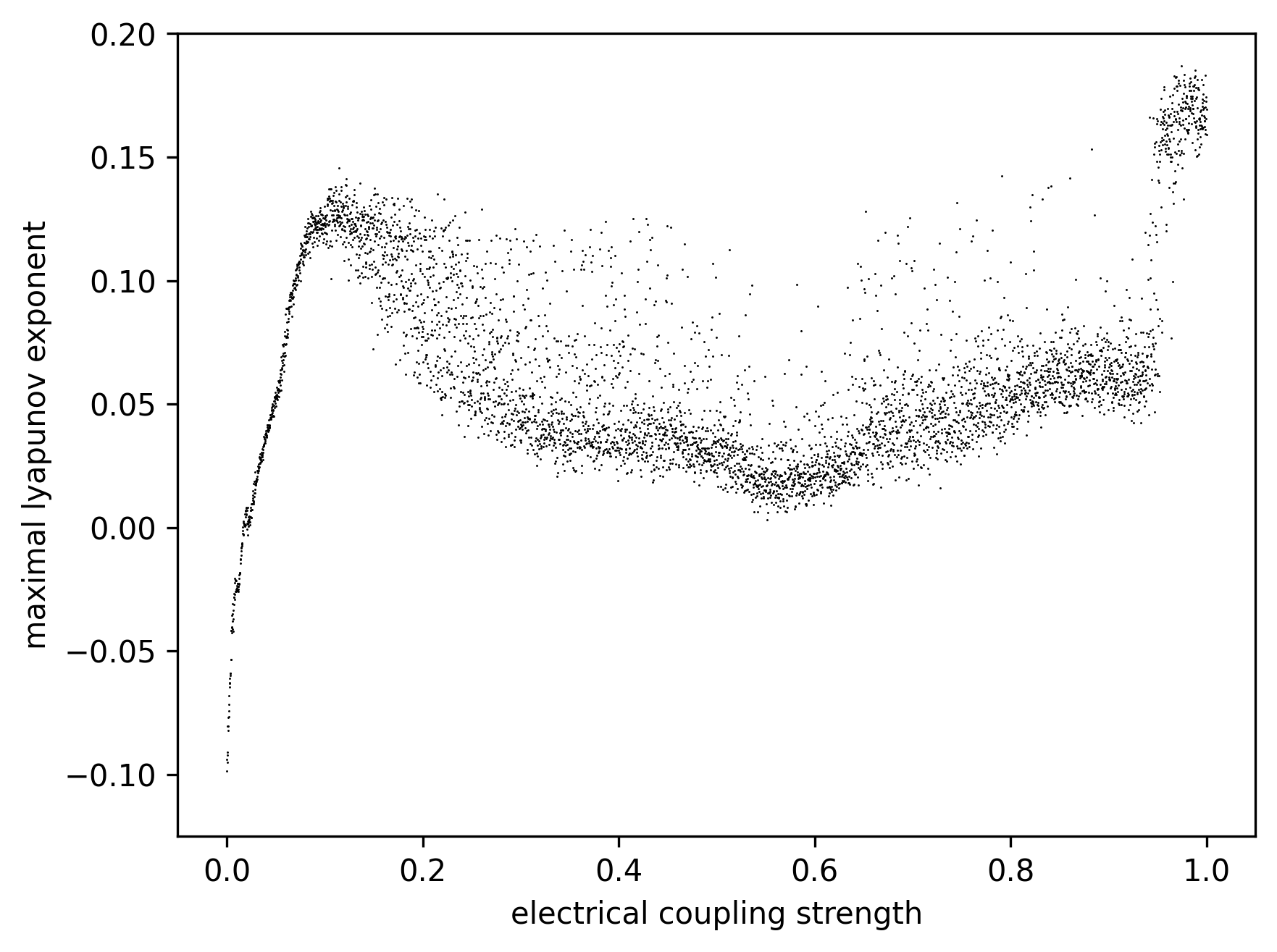
Figure 3: Graph of the maximal Lyapunov exponent $\lambda_{1}$ against the electrical coupling strength $g^{e}$ for the first ring lattice system, with $x_{i,0}\in(-1,1)$, $y_{i,0}=-3.25$, $\sigma_{i}=0.5$, and $\alpha_{i}=4.5$

We will now present our results detailing the dynamics that emerge from the first ring system (different $x_{i,0}$ values, same $y_{i,0}$, $\sigma_{i}$, and $\alpha_{i}$ values). We choose parameters $\sigma_{i}=-0.5$ and $\alpha_{i}=4.5$ for all of the neurons. Additionally, we set the initial slow variable values for all of the neurons to be $y_{i,0}=-3.25$. However, setting the initial fast variable values to be equal would be pointless because then the neurons would have identical dynamics, resulting in no current flow between them. Instead, we choose $x_{i,0}$ variables randomly from the interval $(-1,1)$ .

In Fig. 2, we graph the first thousand iterations of the fast variable orbits of the first eight Rulkov neurons in the ring. We start with uncoupled neurons $g^{e}=0$ in Fig. 2(a), where these neurons with identical parameters are all out of phase in the non-chaotic spiking domain. As expected, because there is no current flow and all of the individual Rulkov neurons are spiking regularly, the maximal Lyapunov exponent $\lambda_{1}$ is negative. When the electrical coupling strength is raised to $g^{e}=0.05$ (Fig. 2(b)), the neurons still spike relatively periodically, but there are some irregularities when one voltage happens to catch onto another. This small $g^{e}$ is enough to make the system chaotic, with $\lambda_{1}\approx 0.0491>0$. Next, we raise the coupling strength significantly to $g^{e}=0.25$, where the ring system now exhibits synchronized chaotic bursting (Fig. 2(c)). This aligns with other computational neuron modelings, where the bursts generally happen in sync with each other but the individual spikes within the bursts are chaotic and unsynchronized [14, 15]. Finally, we take the coupling strength to the extreme with $g^{e}=1$ in Fig. 2(d), where complete chaos ensues ($\lambda_{1}\approx 0.1694$) due to each Rulkov neuron having an overwhelming influence on its nearest neighbors.

A natural question to ask is how the maximal Lyapunov exponent changes as $g^{e}$ is varied, a graph of which is displayed in Fig. 3 for this first system. We notice that the maximal Lyapunov exponents are rather erratic for $g^{e}>0.1$, covering a wide range of values over a small domain of $g^{e}$ values. However, there do exist some general trends. Because the individual neurons in this system are non-chaotic, $\lambda_{1}$ values initially start below zero. As current starts to flow, the range of chaotic spiking is reached (e.g. Fig. 2(b)), where the $\lambda_{1}$ values quickly become positive and reach a maximum. Then, as the synchronized chaotic bursting regime is reached (e.g. Fig. 2(c)), the $\lambda_{1}$ values become much more erratic but exhibit an overall downward trend, which can be attributed to the non-chaotic silence between bursts of spikes. As we reach the extreme values of $g^{e}$ towards the right side of the graph (e.g. Fig. 2(d)), $\lambda_{1}$ shoots up to high and hyperchaotic values.

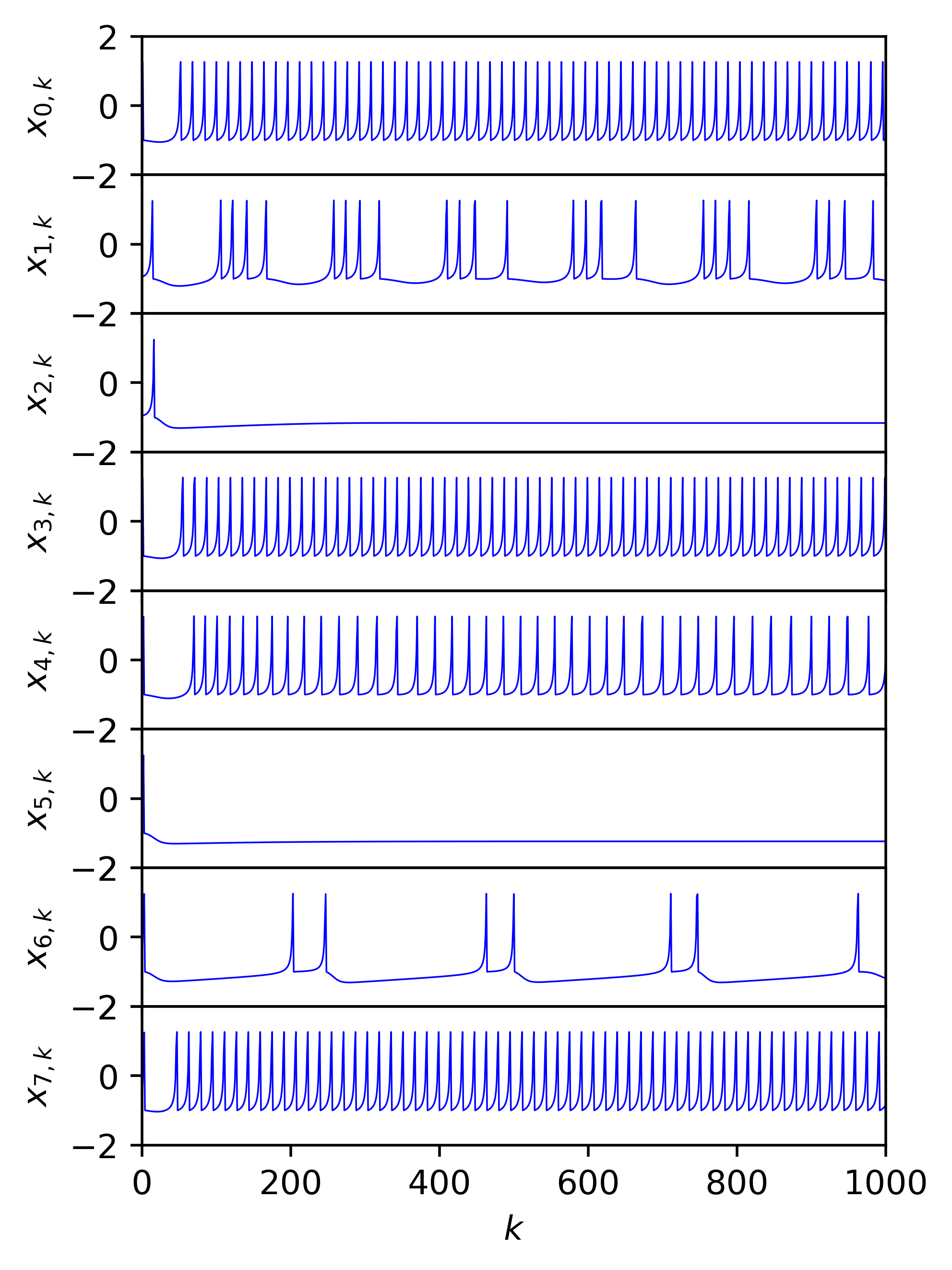
(a) $g^{e}=0$, $\lambda_{1}\approx 0.0644$

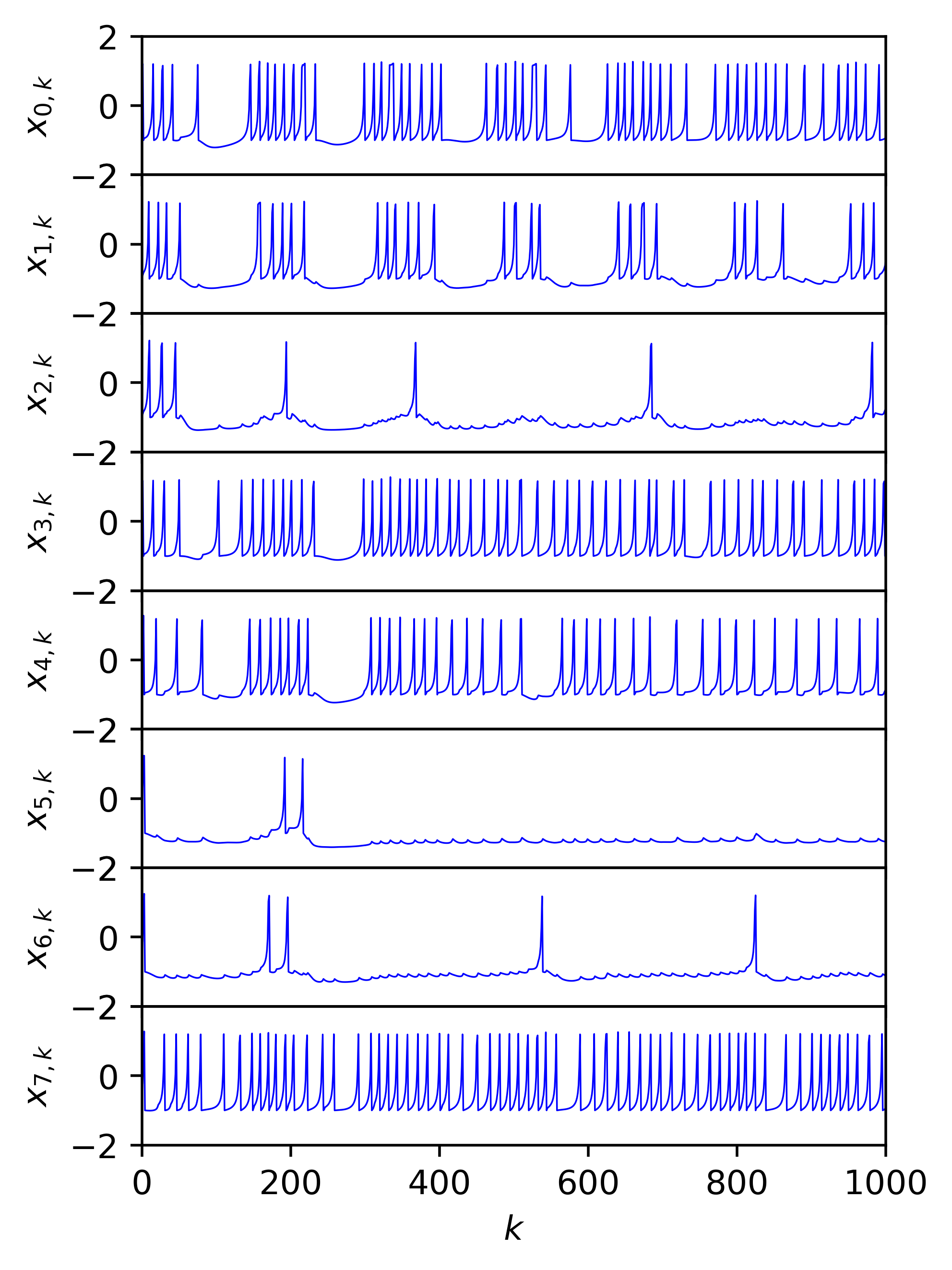
(b) $g^{e}=0.05$, $\lambda_{1}\approx 0.0686$

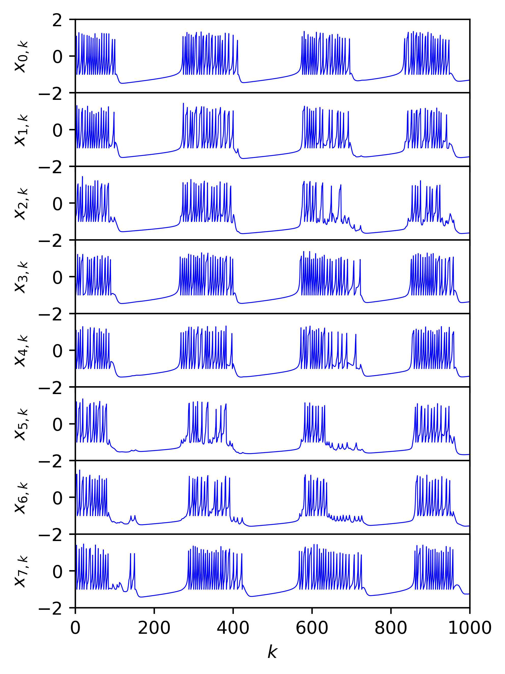
(c) $g^{e}=0.25$, $\lambda_{1}\approx 0.0663$

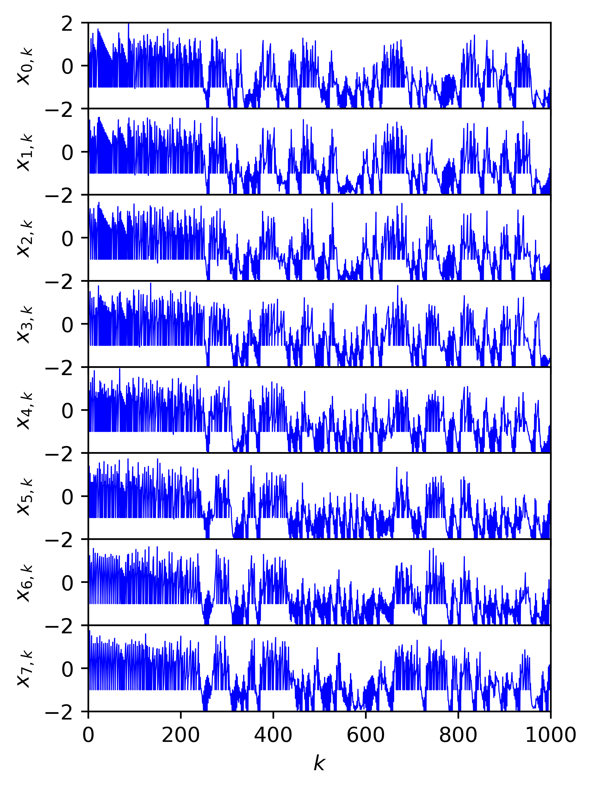
(d) $g^{e}=1$, $\lambda_{1}\approx 0.2003$

Figure 4: Graphs of the fast variable orbits of the first eight neurons in the second ring system, with $x_{i,0}\in(-1,1)$, $y_{i,0}=-3.25$, $\sigma_{i}\in(-1.5,-0.5)$, and $\alpha_{i}=4.5$

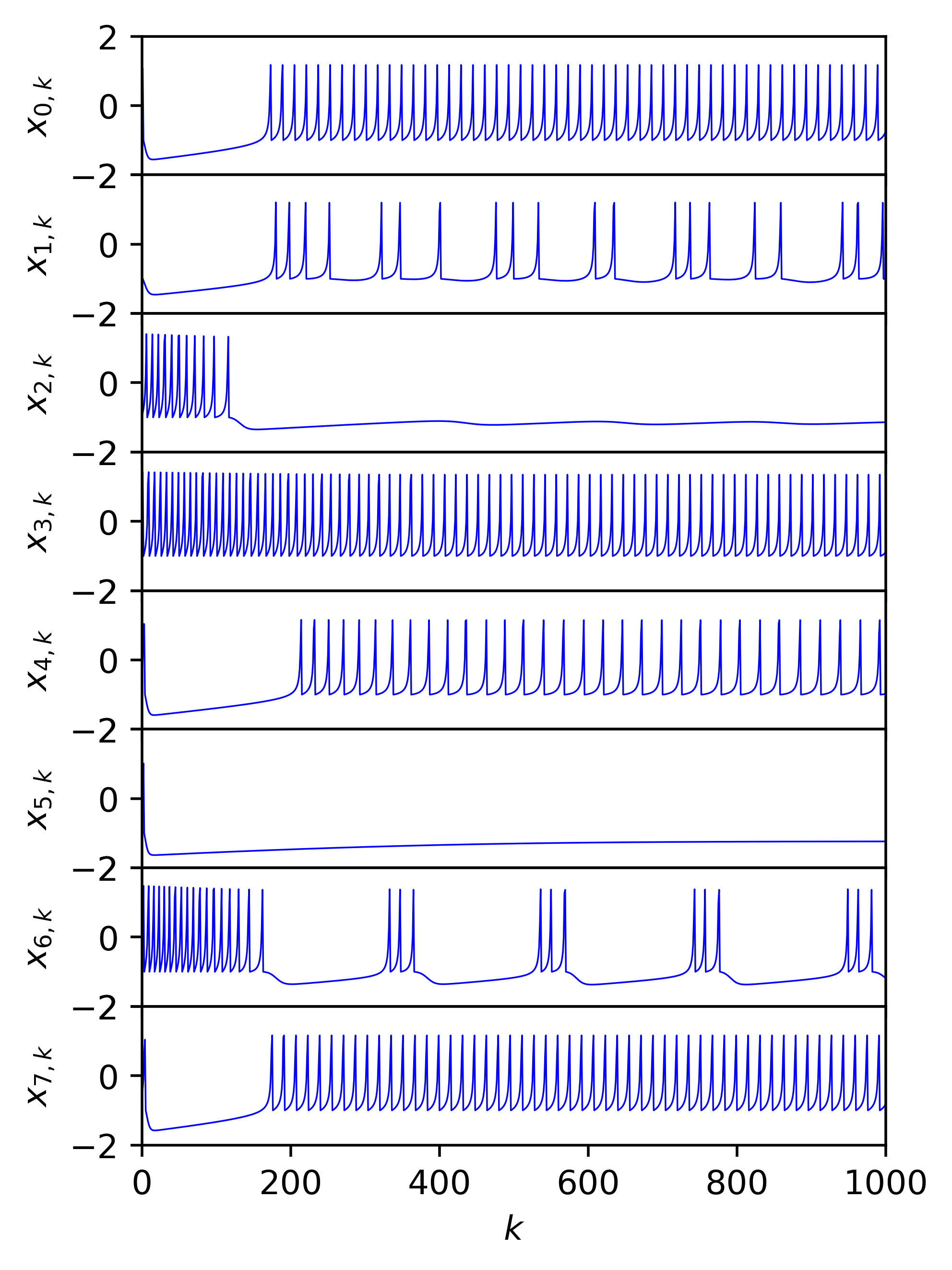
(a) $g^{e}=0$, $\lambda_{1}\approx 0.0469$

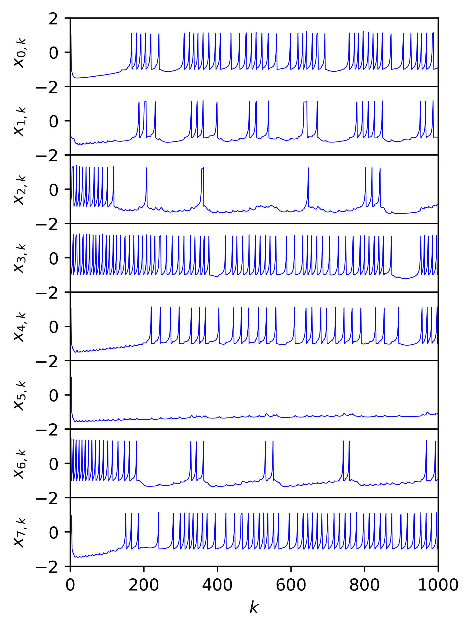
(b) $g^{e}=0.05$, $\lambda_{1}\approx 0.0563$

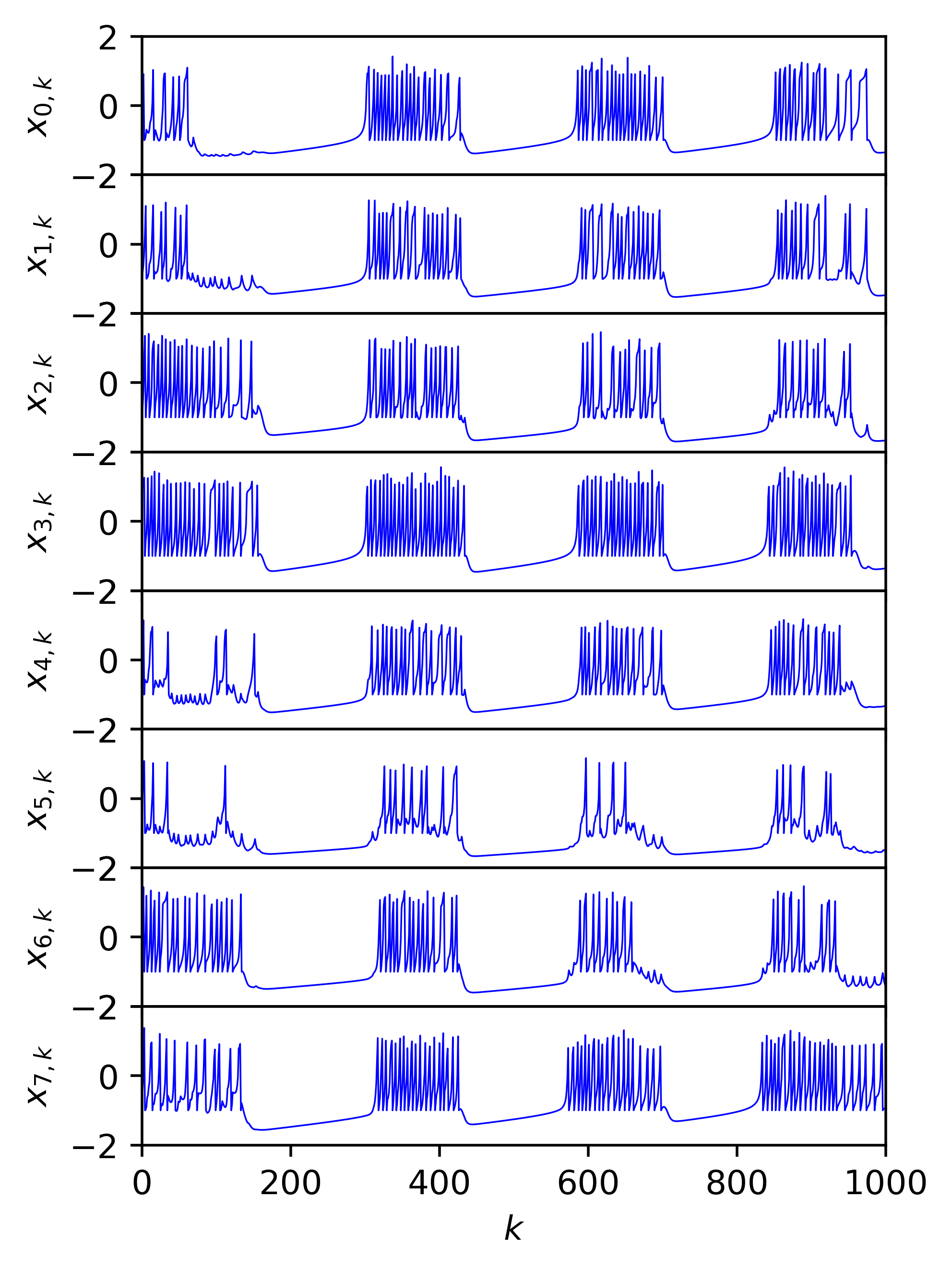
(c) $g^{e}=0.25$, $\lambda_{1}\approx 0.0633$

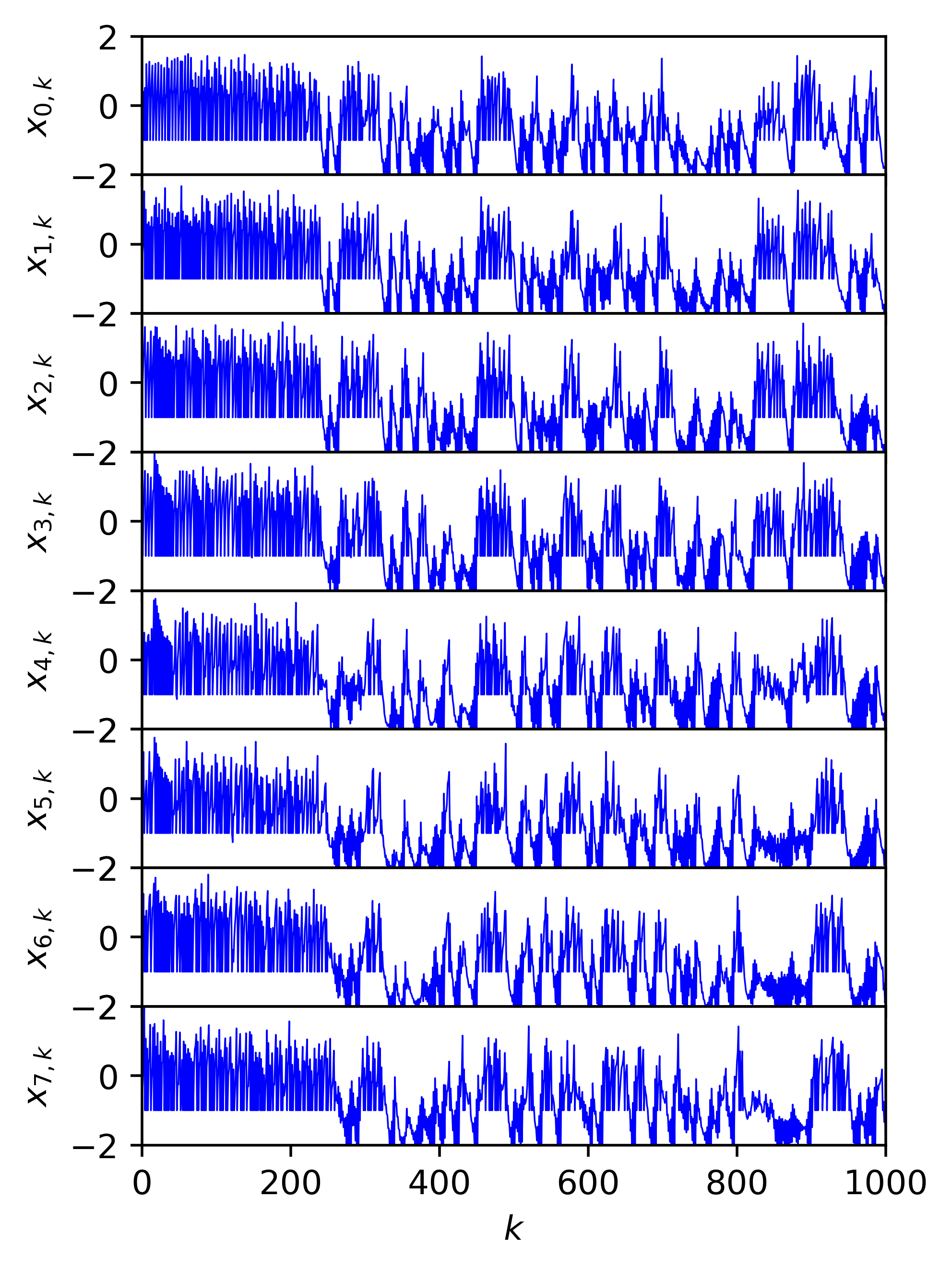
(d) $g^{e}=1$, $\lambda_{1}\approx 0.2053$

Figure 5: Graphs of the fast variable orbits of the first eight neurons in the third ring system, with $x_{i,0}\in(-1,1)$, $y_{i,0}=-3.25$, $\sigma_{i}\in(-1.5,-0.5)$, and $\alpha_{i}\in(4.25,4.75)$

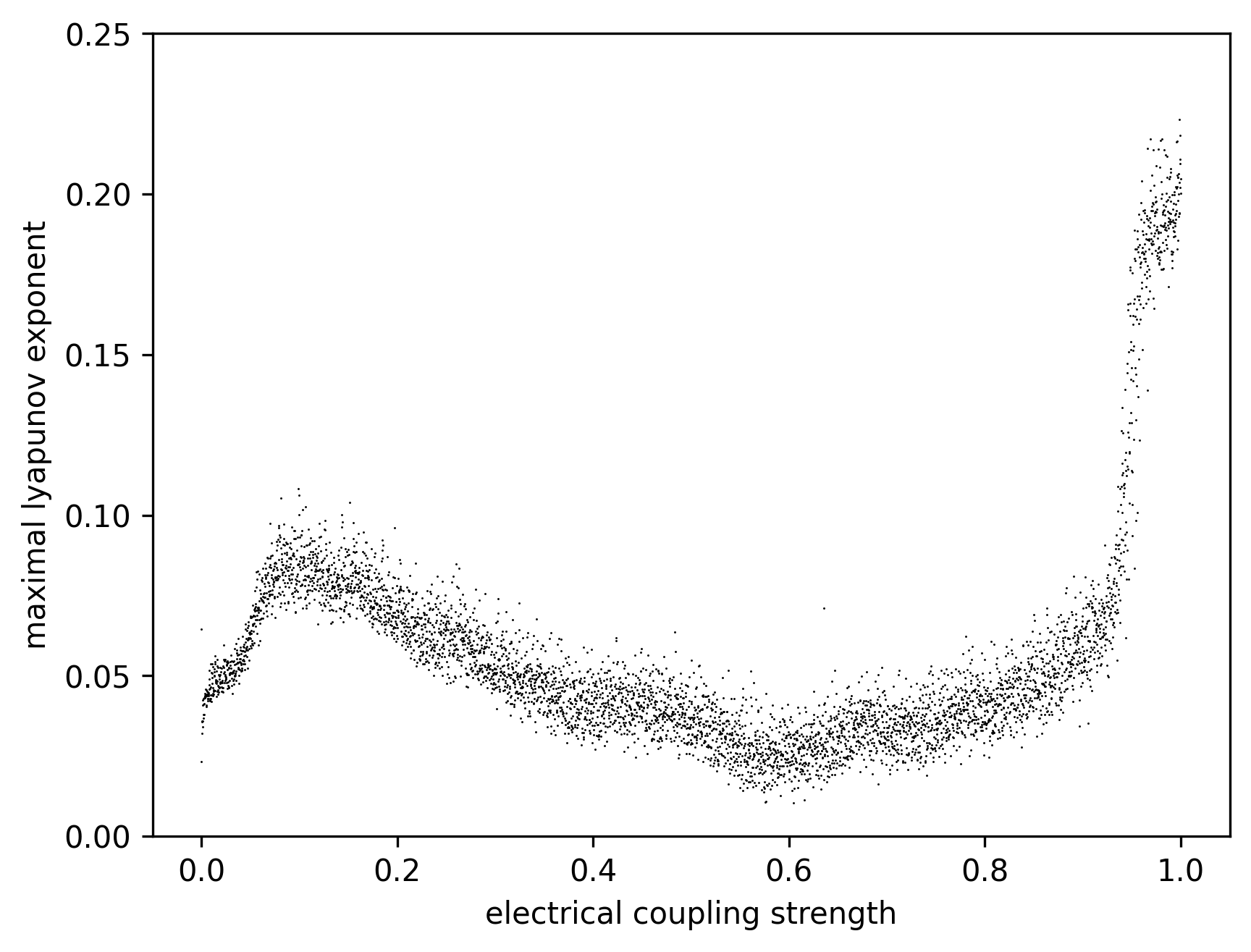
(a) Second system (random $\sigma_{i}$)

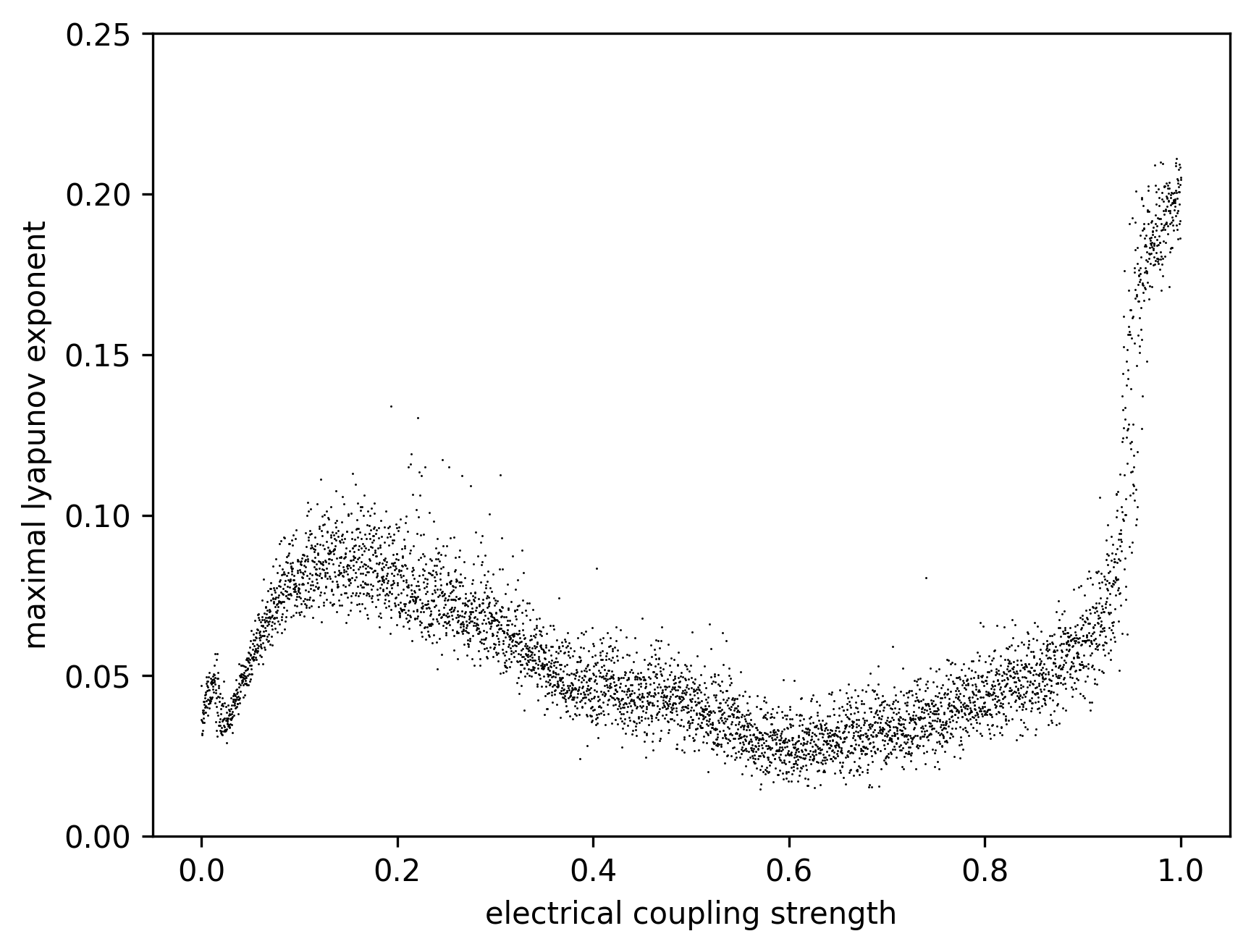
(b) Third system (random $\sigma_{i}$ and $\alpha_{i}$)

Figure 6: Graphs of the maximal Lyapunov exponent $\lambda_{1}$ against the electrical coupling strength $g^{e}$ for the second and third ring systems

We will now examine the second and third ring systems of interest, where different neurons in the ring have different parameters. The second system keeps the same randomly distributed $x_{i,0}$ values (Eq. 17), the same $y_{i,0}=-3.25$ values, and the same $\alpha_{i}=4.5$ values, but it has randomly chosen $\sigma_{i}$ values from the interval $(-1.5,-0.5)$ (Eq. 18). With these parameters, different individual neurons are in the silence, spiking, and bursting domains [14], which can be seen in the visualization of the uncoupled neuron system’s dynamics (Fig. 4(a)).

Finally, the third system we analyze is one where we keep the randomly distributed $x_{i,0}$ and $\sigma_{i}$ values, keep $y_{i,0}=-3.25$, but randomly choose $\alpha_{i}$ values from the interval $(4.25,4.75)$ (Eq. 19). This further varies the distribution of possible behaviors between different neurons in the system. This can be seen in the dynamics of the uncoupled neuron system (Fig. 5(a)), where some neurons exhibit rapid spiking, some burst occasionally, and some are silent.

In Figs. 4 and 5, we graph the fast variable orbits of the first eight neurons in the ring using the same electrical coupling strength values as the first system: $g^{e}=0,0.05,0.25,1$. Comparing both of these systems to the first system, similar patterns emerge among them. For $g^{e}=0.05$, the adjacent neurons start to have some effect on each other, but the overall dynamical picture remains the same. Raising the electrical coupling strength up to $g^{e}=0.25$, all the neurons undergo synchronized chaotic bursting, and going to the extreme $g^{e}=1$, complete chaos ensues. An interesting observation that is even clearer in these visualizations is neurons’ direct influence on their adjacent partners. For instance, in Figs. 4(b) and 5(c), spiking in one neuron is reflected in adjacent neurons with smaller spikes during a period of silence.

Fig. 6 presents a visualization of the maximal Lyapunov exponents of these two systems for many values of $g^{e}$. An evident difference when comparing these graphs to the graph in Fig. 3 is that $\lambda_{1}>0$ for all the $g^{e}$ values. This is because even when the neurons are uncoupled, some of the individual neurons in the ring are chaotic. However, the graphs of the maximal Lyapunov exponents for all three of our systems have similar shapes, the major differences being when the neurons are weakly coupled and operating under their own parameters. Past this weak coupling domain, all three graphs in Figs. 3 and 6 follow the increase up to chaotic spiking, the swoop down as synchronized chaotic bursts occur, and the shoot up as the extreme values of $g^{e}$ are approached. Therefore, despite making individual neurons exhibit drastically different dynamics from their neighbors, coupling makes the systems exhibit similar dynamics.

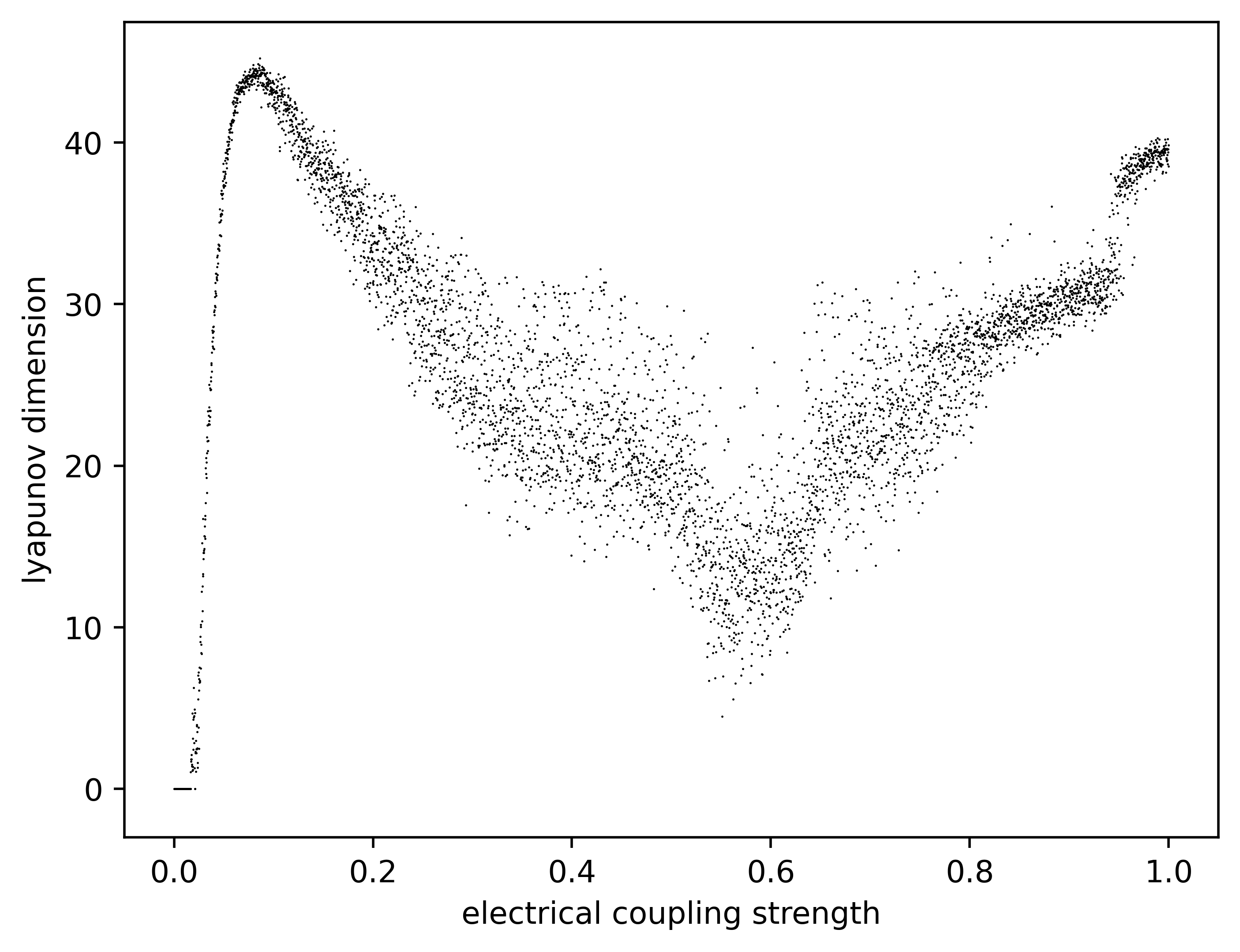
(a) First ring lattice system

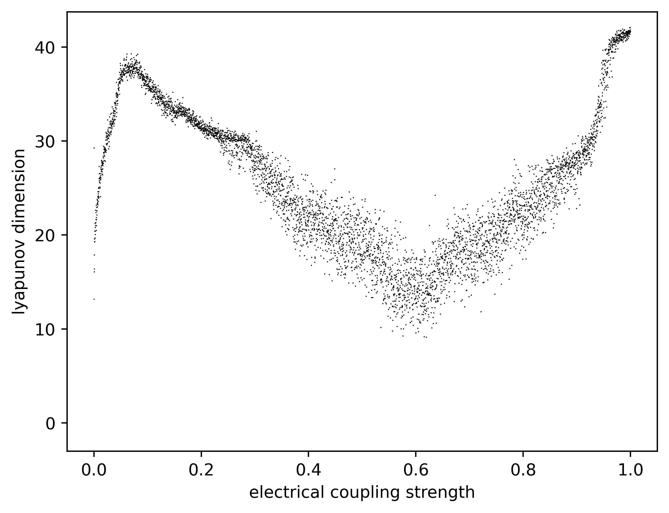
(b) Second ring lattice system

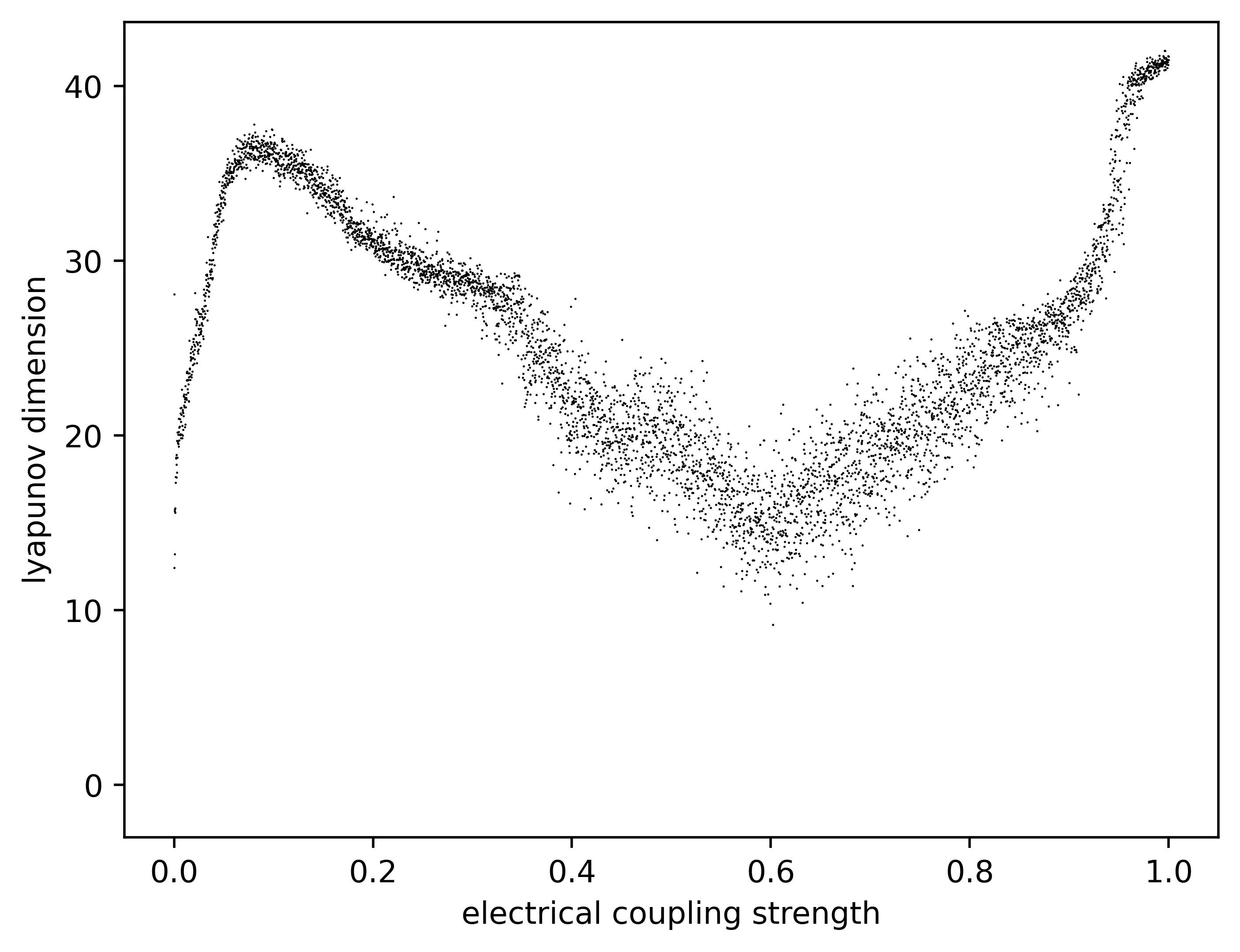
(c) Third ring lattice system

Figure 7: Graphs of the Lyapunov dimension $d_{l}$ against the electrical coupling strength $g^{e}$ for three ring lattice systems of $\zeta=30$ electrically coupled Rulkov neurons

III Fractal geometry of attractors

In Sec. II, we found that the three Rulkov neuron ring lattice systems that we examined nearly always exhibit chaotic dynamics with positive maximal Lyapunov exponents. Therefore, we can conclude that these systems evolve towards some chaotic attractor in 60-dimensional state space. Of course, we cannot visualize a geometrical object embedded in 60-dimensional space, so in this section, we will present a brief analysis of the geometry of these strange attractors by approximating their fractal dimensions using the Kaplan-Yorke conjecture, which asserts that the Lyapunov spectrum of the orbit on an attractor is directly related to the attractor’s dimension [41]. Assuming that the Lyapunov spectrum is ordered from greatest to least, let $\kappa$ be the largest index such that

$$\sum_{i=1}^{\kappa}\lambda_{i}\geq 0.$$ (11)

Then, the Lyapunov dimension $d_{l}$ is defined as

$$d_{l}=\kappa+\frac{1}{|\lambda_{\kappa+1}|}\sum_{i=1}^{\kappa}\lambda_{i}.$$ (12)

The Kaplan-Yorke conjecture states that the Lyapunov dimension of an attractor is equal to its true fractal dimension $d$ [42].

Using the full Lyapunov spectrums of the ring lattice systems we computed in Sec. II, we can calculate the Lyapunov dimensions of the three systems using Eqs. 11 and 12. Then, we can make graphs similar to the ones in Figs. 3 and 6 by plotting the values of $d_{l}$ for many different values of $g^{e}$, which is displayed in Fig. 7.

We can immediately see that all the chaotic attractors of these three systems are fractal since are spread out among different real values, not sticking to any defined integers. The only true integer dimensions in these graphs are at the very left of Fig. 7(a), where there are some attractors that have dimension 0. These are associated with the non-chaotic periodic orbit attractors at the left of Fig. 3, which consist of a finite number of zero-dimensional points. One example of these orbits is displayed in the regular spiking of Fig. 2(a). Another notable observation is that these attractors take up a sizable amount of state space. Because the state space of this system is so large, we might expect the attractors to take up only a small fraction of it, but instead, the strange attractors take up a substantial portion of it for many values of $g^{e}$, with some of the largest of these attractors taking up close to 45 of the 60 total dimensions.

Comparing Fig. 7 to the graphs of $\lambda_{1}$ vs. $g^{e}$ in Figs. 3 and 6, we can see that the Lyapunov dimension $d_{l}$ follows a similar pattern of increasing through the chaotic spiking domain, decreasing as the neurons start to burst in sync with each other, then increasing again as complete chaos is reached. This is to be expected because the Lyapunov dimension is calculated directly from the set of Lyapunov exponents. There is also a similarity in how the $d_{l}$ and $\lambda_{1}$ values are distributed across the different systems. Specifically, the $\lambda_{1}$ values are more erratic and spread out in the first system than they are in the second and third systems, which is also reflected in the $d_{l}$ values to some degree. Namely, the values of $d_{l}$ in Fig. 7(a) are more vertically spread out in the synchronized bursting domain. However, there are some very clear differences between the trends of the maximal Lyapunov exponent $\lambda_{1}$ and the Lyapunov dimension $d_{l}$. The most apparent difference is in comparing the peaks of the $\lambda_{1}$ vs. $g^{e}$ graphs and the $d_{l}$ vs. $g^{e}$ graphs, with both peaks in both graphs being associated with chaotic spiking around $g^{e}=0.1$ and complete chaos around $g^{e}=1$. In the $\lambda_{1}$ vs. $g^{e}$ graphs, the peak in the region of complete chaos is always higher than the peak in the region of chaotic spiking, a fact that is extremely apparent in Fig. 6 (the second and third ring systems), where the peaks on the right dwarf the peaks on the left. However, in the graphs of $d_{l}$ vs. $g^{e}$, the peaks are similar in height, and in Fig. 7(a) (the first ring system), the left peak is actually higher than the right peak. This means that, for this system, the chaotic spiking attractor that appears when the electrical coupling strength is relatively small takes up more state space than the attractor that appears when the electrical coupling strength is very large, which is a somewhat surprising result. This comparison makes it clear that although $\lambda_{1}$ quantifies how chaotic the ring lattice attractors are, it does not directly correlate to their size or strangeness. For that, as the Kaplan-Yorke conjecture indicates, we need the entire Lyapunov spectrum.

IV Conclusions

We investigated the dynamics and geometry that emerged from a model consisting of a ring of electrically coupled non-chaotic Rulkov neurons. We performed numerical simulations of the dynamics of three ring lattice systems of $\zeta=30$ neurons and found that a variety of chaotic behaviors emerged from individual non-chaotic neurons, observing chaotic spiking, synchronized chaotic bursts, and complete chaos. By calculating the $2\zeta\times 2\zeta$ Jacobian matrix, we quantified the chaos of the ring systems by computing their maximal Lyapunov exponents for many different electrical coupling strength values. Using a QR factorization method of computing the entire Lyapunov spectrums of the systems, we approximated the fractal dimensions of the attractors in 60-dimensional state space by means of the Kaplan-Yorke conjecture. We found that all the chaotic attractors of the three systems were fractal and that for some electrical coupling strength values, the attractors took up significant portions of 60-dimensional state space. Comparing the Lyapunov dimensions of the ring lattice systems to their maximal Lyapunov exponents, we also found that while the Lyapunov dimensions followed a similar pattern of increasing and decreasing as we varied the electrical coupling strength, the two quantities were not directly associated with each other.

Our study in ring lattice systems of non-chaotic Rulkov neurons sets a precedent for how the chaotic dynamics and fractal geometry of different neuron lattice models may be analyzed and quantified. Specifically, our calculation of the complex Jacobian matrix of the ring model can be naturally extended to more complex lattices of neurons, such as a mesh, torus, or sphere, as well as an all-to-all coupled system. Although these have been studied in the context of a mean field of chaotic Rulkov neurons [15], this has never been done with the more experimentally applicable electrical coupling of Rulkov neurons to the best of our knowledge. With more current connections, we suspect that more interesting hyperchaotic dynamics may appear. Additional research may be done in trying to observe these complex dynamics in real neurons, building on the existing experimental work with coupled biological neurons [43, 44, 45].

Appendix A Jacobian matrix derivation

In this appendix, we outline a sketch of the derivation of the Jacobian matrix for a Rulkov ring lattice system governed by the iteration function in Eq. 10 . Specifically, we derive the $mp$th entry of $J(\mathbf{X})$:

$$J_{mp}(\mathbf{X})=\frac{\partial F^{[m]}}{\partial X^{[p]}}.$$ (13)

From Eq. 9, it is clear that when $p$ is odd, we are differentiating with respect to the fast variable of the neuron with index $i=(p-1)/2$, and when $p$ is even, we are differentiating with respect the slow variable of the neuron with index $i=p/2-1$. Similarly, from Eq. 10, when $m$ is odd, we are differentiating the piecewise fast variable function $f$ of the neuron with index $i=(m-1)/2$, and when $m$ is even, we are differentiating the slow variable function of the neuron with index $i=m/2-1$.

Let us first consider even $m$, or $m\bmod 2=0$. By Eqs. 4 and 8, the slow variable iteration function for neuron $i=m/2-1$ is

$$F^{[m]}=y_{m/2-1}-\mu x_{m/2-1}+\mu\Bigg{[}\sigma_{m/2-1}+\frac{g^{e}}{2}(x_{(m/2-2)\bmod\zeta}+x_{(m/2)\bmod\zeta}-2x_{m/2-1})\Bigg{]}.$$ (14)

This function only depends on $y_{m/2-1}$, $x_{m/2-1}$, $x_{(m/2-2)\bmod\zeta}$, and $x_{(m/2)\bmod\zeta}$, so the derivative with respect to any other variable will vanish. Therefore, we need only determine the values of $p$ that will make $X^{[p]}$ equal one of these variables that yield a non-vanishing derivative, where careful attention must be paid to the values of $m$ that are near the loop-around point of the ring.

For odd $m$ ($m\bmod 2=1$), we are differentiating the fast variable iteration function of neuron $i=(m-1)/2$. Therefore, by Eqs. 2, 4, and 8,

$$\begin{split}F^{[m]}&=f(x_{(m-1)/2},y_{(m-1)/2}+\mathfrak{C}_{(m-1)/2};\alpha_{(m-1)/2})\\[7.11317pt] &=\begin{cases}\frac{\alpha_{(m-1)/2}}{1-x_{(m-1)/2}}+y_{(m-1)/2}+\frac{g^{e}}{2}(x_{[(m-3)/2]\bmod\zeta}+x_{[(m+1)/2]\bmod\zeta}-2x_{(m-1)/2}),&x_{(m-1)/2}\leq 0\vskip 14.22636pt\\ \alpha_{(m-1)/2}+y_{(m-1)/2}+\frac{g^{e}}{2}(x_{[(m-3)/2]\bmod\zeta}+x_{[(m+1)/2]\bmod\zeta}-2x_{(m-1)/2}),&0<x_{(m-1)/2}<\alpha_{(m-1)/2}\\ &+y_{(m-1)/2}+\mathfrak{C}_{(m-1)/2}\vskip 14.22636pt\\ -1,&x_{(m-1)/2}\geq\alpha_{(m-1)/2}\\ &+y_{(m-1)/2}+\mathfrak{C}_{(m-1)/2}\\ \end{cases}.\end{split}$$ (15)

In the case where $x_{(m-1)/2}\leq 0$, the only variables present are $y_{(m-1)/2}$, $x_{(m-1)/2}$, $x_{[(m-3)/2]\bmod\zeta}$, and $x_{[(m+1)/2]\bmod\zeta}$, so we can systematically determine the values of $p$ that yield non-zero derivatives in a similar fashion to the odd $m$ function. In the case where $0<x_{(m-1)/2}<\alpha_{(m-1)/2}+y_{(m-1)/2}+\mathfrak{C}_{(m-1)/2}$, we have different non-zero derivatives since the function piece is different, but this piece depends on the same variables as the first piece, so the same relevant $p$ values apply. In the case where $x_{(m-1)/2}\geq\alpha_{(m-1)/2}+y_{(m-1)/2}+\mathfrak{C}_{(m-1)/2}$, the derivative with respect to any variable is trivial. Putting all of this together yields the Jacobian entry $J_{mp}(\mathbf{X})$ central to the Lyapunov spectrum calculation for a Rulkov ring lattice system:

$$J_{mp}(\mathbf{X})=\begin{cases}\begin{cases}\begin{cases}1,&\hskip 9.24706pt\text{if }p=m+1,\\ \frac{\alpha_{(m-1)/2}}{(1-x_{(m-1)/2})^{2}}-g^{e},&\hskip 9.24706pt\text{if }p=m,\\ g^{e}/2,&\begin{cases}\text{if }p=m-2,\\ \phantom{if}\text{ and }m\neq 1,\\ \text{or }p=2\zeta-1,\\ \phantom{if}\text{ and }m=1,\\ \text{or }p=m+2,\\ \phantom{if}\text{ and }m\neq 2\zeta-1,\\ \text{or }p=1,\\ \phantom{if}\text{ and }m=2\zeta-1,\end{cases}\\ 0,&\hskip 9.24706pt\text{otherwise,}\end{cases}\text{for }x_{(m-1)/2}\leq 0,\\ \\ \\ \begin{cases}1,&\hskip 63.30754pt\text{if }p=m+1,\\ -g^{e},&\hskip 63.30754pt\text{if }p=m,\\ g^{e}/2,&\hskip 54.06006pt\begin{cases}\text{if }p=m-2,\\ \phantom{if}\text{ and }m\neq 1,\\ \text{or }p=2\zeta-1,\\ \phantom{if}\text{ and }m=1,\\ \text{or }p=m+2,\\ \phantom{if}\text{ and }m\neq 2\zeta-1,\\ \text{or }p=1,\\ \phantom{if}\text{ and }m=2\zeta-1,\end{cases}\stackunder{\text{for $0<x_{(m-1)/2}<\alpha_{(m-1)/2}$}}{\text{$+y_{(m-1)/2}+\mathfrak{C}_{(m-1)/2},$}}\\ 0,&\hskip 63.30754pt\text{otherwise,}\end{cases}\\ \\ \\ 0,\hskip 190.20659pt\text{for}\stackunder{x_{(m-1)/2}\geq\alpha_{(m-1)/2}}{+y_{(m-1)/2}+\mathfrak{C}_{(m-1)/2},}\\ \end{cases}&\text{when }m\bmod 2=1\\ \\ \\ \begin{cases}1,&\hskip 19.0633pt\text{if }p=m\\ -\mu(1+g^{e}),&\hskip 19.0633pt\text{if }p=m-1\\ \mu g^{e}/2,&\hskip 9.81622pt\begin{cases}\text{if }p=m-3\\ \phantom{if}\text{ and }m\neq 2\\ \text{or }p=2\zeta-1\\ \phantom{if}\text{ and }m=2\\ \text{or }p=m+1\\ \phantom{if}\text{ and }m\neq 2\zeta\\ \text{or }p=1\\ \phantom{if}\text{ and }m=2\zeta\end{cases}\\ 0,&\hskip 19.0633pt\text{otherwise,}\end{cases}&\text{when }m\bmod 2=0\end{cases}.$$ (16)

Appendix B Random initial states and parameters

In all three ring lattice systems we studied, we used random initial states and parameters. In this appendix, we list these random values for the sake of reproducibility of results. We use the notation $\bm{\alpha}=(\alpha_{1},\ldots,\alpha_{\zeta})$ and $\bm{\sigma}=(\sigma_{1},\ldots,\sigma_{\zeta})$

In all three ring lattice systems, we use the initial state

$$\begin{split}\mathbf{X}_{0}&=(0.68921784,-3.25,-0.94561073,-3.25,-0.95674631,-3.25,0.91870134,-3.25,\\ &\mathrel{\phantom{=}}-0.32012381,-3.25,-0.23746836,-3.25,-0.43906743,-3.25,-0.48671017,-3.25,\\ &\mathrel{\phantom{=}}-0.37578533,-3.25,-0.00613823,-3.25,0.25990663,-3.25,-0.54103868,-3.25,\\ &\mathrel{\phantom{=}}0.12110471,-3.25,0.71202085,-3.25,0.689336,-3.25,-0.03260047,-3.25,\\ &\mathrel{\phantom{=}}-0.90907325,-3.25,0.93270227,-3.25,0.51953315,-3.25,-0.46783677,-3.25,\\ &\mathrel{\phantom{=}}-0.96738424,-3.25,-0.50828432,-3.25,-0.60388469,-3.25,-0.56644705,-3.25,\\ &\mathrel{\phantom{=}}-0.42772621,-3.25,0.7716625,-3.25,-0.60336517,-3.25,0.88158364,-3.25,\\ &\mathrel{\phantom{=}}0.0269842,-3.25,0.42512831,-3.25),\end{split}$$ (17)

with $x_{i,0}\in(-1,1)$.
In the second and third ring systems, we use the $\bm{\sigma}$ vector

$$\begin{split}\bm{\sigma}&=(-0.63903048,-0.87244087,-1.16110093,-0.63908737,-0.73103576,-1.23516699,\\ &\mathrel{\phantom{=}}-1.09564519,-0.57564289,-0.75055299,-1.01278976,-0.61265545,-0.75514189,\\ &\mathrel{\phantom{=}}-0.89922568,-1.24012127,-0.87605023,-0.94846269,-0.78963971,-0.94874874,\\ &\mathrel{\phantom{=}}-1.31858036,-1.34727902,-0.7076453,-1.10631486,-1.33635792,-1.48435264,\\ &\mathrel{\phantom{=}}-0.76176103,-1.17618267,-1.10236959,-0.66159308,-1.27849639,-0.9145025),\end{split}$$ (18)

with $\sigma_{i}\in(-1.5,-0.5)$.
In the third ring system, we use the $\bm{\alpha}$ vector

$$\begin{split}\bm{\alpha}&=(4.31338267,4.3882788,4.6578449,4.67308374,4.28873181,4.26278301,\\ &\mathrel{\phantom{=}}4.73065817,4.29330435,4.44416548,4.66625973,4.26243104,4.65881579,\\ &\mathrel{\phantom{=}}4.68086764,4.44092086,4.49639124,4.55500032,4.33389054,4.38869161,\\ &\mathrel{\phantom{=}}4.57278526,4.62717616,4.62025928,4.49780551,4.46750298,4.49561326,\\ &\mathrel{\phantom{=}}4.66902393,4.60858869,4.6027906,4.40563641,4.54198743,4.49388045),\end{split}$$ (19)

with $\alpha_{i}\in(4.25,4.75)$.

References

- Izhikevich [1999] E. M. Izhikevich, Neural excitability, spiking and bursting, International Journal of Bifurcation and Chaos 10, 1171 (1999).
- Hodgkin and Huxley [1952] A. L. Hodgkin and A. F. Huxley, A quantitative description of membrane current and its application to conduction and excitation in nerve, The Journal of Physiology 117, 500 (1952).
- Chay [1985] T. R. Chay, Chaos in a three-variable model of an excitable cell, Physica D: Nonlinear Phenomena 16, 233 (1985).
- Buchholtz et al. [1992] F. Buchholtz, J. Golowasch, I. R. Epstein, and E. Marder, Mathematical model of an identified stomatogastric ganglion neuron, Journal of Neurophysiology 67, 332 (1992).
- Izhikevich [2003a] E. M. Izhikevich, Simple model of spiking neurons, IEEE Transactions on Neural Networks 14, 1569 (2003a).
- FitzHugh [1961] R. FitzHugh, Impulses and physiological states in theoretical models of nerve membrane, Biophysical Journal 1, 445–466 (1961).
- Hindmarsh and Rose [1984] J. L. Hindmarsh and R. M. Rose, A model of neuronal bursting using three coupled first order differential equations, Proceedings of the Royal Society B 221, 87 (1984).
- Rinzel [1987] J. Rinzel, A formal classification of bursting mechanisms in excitable systems (Springer, Berlin, Heidelberg, 1987) pp. 267–281.
- Izhikevich and Hoppensteadt [2004] E. M. Izhikevich and F. Hoppensteadt, Classification of bursting mappings, International Journal of Bifurcation and Chaos 14, 3847 (2004).
- Izhikevich [2003b] E. Izhikevich, Simple model of spiking neurons, IEEE Transactions on Neural Networks 14, 1569 (2003b).
- Courbage et al. [2007] M. Courbage, V. I. Nekorkin, and L. V. Vdovin, Chaotic oscillations in a map-based model of neural activity, Chaos 17 (2007).
- Omelchenko et al. [2011] I. Omelchenko, M. Rosenblum, and A. Pikovsky, Synchronization of slow-fast systems, The European Physical Journal Special Topics 191, 3 (2011).
- Izhikevich [2004] E. Izhikevich, Which model to use for cortical spiking neurons?, IEEE Transactions on Neural Networks 15, 1063 (2004).
- Rulkov [2002] N. F. Rulkov, Modeling of spiking-bursting neural behavior using two-dimensional map, Physical Review E 65 (2002).
- Rulkov [2001] N. F. Rulkov, Regularization of synchronized chaotic bursts, Physical Review Letters 86, 183 (2001).
- Ibarz et al. [2011] B. Ibarz, J. M. Casado, and M. A. F. Sanjuán, Map-based models in neuronal dynamics, Physics Reports 501, 1 (2011).
- de Vries [2001] G. de Vries, Bursting as an emergent phenomenon in coupled chaotic maps, Physical Review E 64 (2001).
- Luo et al. [2024] D. Luo, C. Wang, Q. Deng, and Y. Sun, Dynamics in a memristive neural network with three discrete heterogeneous neurons and its application, Nonlinear Dynamics (2024).
- Min et al. [2024] F. Min, G. Zhai, S. Yin, and J. Zhong, Switching bifurcation of a Rulkov neuron system with relu-type memristor, Nonlinear Dynamics 112 (2024).
- Bao et al. [2023] H. Bao, K. Li, J. Ma, Z. Hua, Q. Xu, and B. Bao, Memristive effects on an improved discrete Rulkov neuron model, Science China Technological Sciences 66 (2023).
- de Pontes et al. [2008] J. de Pontes, R. Viana, S. Lopes, C. Batista, and A. Batista, Bursting synchronization in non-locally coupled maps, Physica A: Statistical Mechanics and its Applications 387 (2008).
- Wang and Cao [2015] C. Wang and H. Cao, Stability and chaos of Rulkov map-based neuron network with electrical synapse, Communications in Nonlinear Science and Numerical Simulation 20 (2015).
- López et al. [2023] J. López, M. Coccolo, R. Capeáns, and M. A. Sanjuán, Controlling the bursting size in the two-dimensional Rulkov model, Communications in Nonlinear Science and Numerical Simulation 120 (2023).
- Budzinski et al. [2021] R. Budzinski, S. Lopes, and C. Masoller, Symbolic analysis of bursting dynamical regimes of Rulkov neural networks, Neurocomputing 441 (2021).
- Ge and Cao [2021] P. Ge and H. Cao, Intermittent evolution routes to the periodic or the chaotic orbits in Rulkov map featured, Chaos 31 (2021).
- Njitacke et al. [2024] Z. T. Njitacke, C. N. Takembo, G. Sani, N. Marwan, R. Yamapi, and J. Awrejcewicz, Hidden and self-excited firing activities of an improved Rulkov neuron, and its application in information patterns, Nonlinear Dynamics 112 (2024).
- Ding et al. [2024] D. Ding, Y. Niu, Z. Yang, J. Wang, W. Wang, M. Wang, and F. Jin, Extreme multi-stability and microchaos of fractional-order memristive Rulkov neuron model considering magnetic induction and its digital watermarking application, Nonlinear Dynamics 112 (2024).
- Note [1] In the original paper that introduces the Rulkov map [14], the parameter is used, but we use the slightly modified form from Ref. [16].
- Hu and Cao [2016] D. Hu and H. Cao, Stability and synchronization of coupled Rulkov map-based neurons with chemical synapses, Communications in Nonlinear Science and Numerical Simulation 35, 105 (2016).
- Rakshit et al. [2018] S. Rakshit, A. Ray, B. K. Bera, and D. Ghosh, Synchronization and firing patterns of coupled Rulkov neuronal map, Nonlinear Dynamics 94, 785–805 (2018).
- Sun and Cao [2016] H. Sun and H. Cao, Complete synchronization of coupled Rulkov neuron networks, Nonlinear Dynamics 84, 2423–2434 (2016).
- Marghoti et al. [2023] G. Marghoti, F. A. S. Ferrari, R. L. Viana, S. R. Lopes, and T. de Lima Prado, Coupling dependence on chaos synchronization process in a network of Rulkov neurons, International Journal of Bifurcation and Chaos 33 (2023).
- Banerjee et al. [2017] R. Banerjee, B. K. Bera, D. Ghosh, and S. K. Dana, Enhancing synchronization in chaotic oscillators by induced heterogeneity, The European Physical Journal Special Topics 226, 1893–1902 (2017).
- Chen et al. [2008] H. Chen, J. Zhang, and J. Liu, Enhancement of neuronal coherence by diversity in coupled Rulkov-map models, Physica A: Statistical Mechanics and its Applications 387, 1071 (2008).
- Osipov et al. [2005] G. V. Osipov, M. V. Ivanchenko, J. Kurths, and B. Hu, Synchronized chaotic intermittent and spiking behavior in coupled map chains, Physical Review E 71 (2005).
- Eckmann and Ruelle [1985] J.-P. Eckmann and D. Ruelle, Ergodic theory of chaos and strange attractors, Reviews of Modern Physics 57, 617 (1985).
- Sandri [1996] M. Sandri, Numerical calculation of Lyapunov exponents, The Mathematica Journal 6, 78 (1996).
- Le [2024] B. Le, Describing chaotic systems (2024), arXiv:2407.07919 [math.GM] .
- Le and Gandhi [2024] B. B. Le and N. A. Gandhi, Exploring geometrical properties of chaotic systems through an analysis of the Rulkov neuron maps (2024), arXiv:2406.08385 [nlin.CD] .
- Note [2] The specific random initial states and parameters we use are listed in Appx. B.
- Kaplan and Yorke [1979] J. L. Kaplan and J. A. Yorke, Chaotic behavior of multidimensional difference equations, Functional Differential Equations and Approximation of Fixed Points 730, 204–227 (1979).
- Nichols et al. [2003] J. M. Nichols, M. D. Todd, M. Seaver, S. T. Trickey, L. M. Pecora, and L. Moniz, Controlling system dimension: A class of real systems that obey the Kaplan–Yorke conjecture, Proceedings of the National Academy of Sciences 100, 15299 (2003).
- Elson et al. [1998] R. C. Elson, A. I. Selverston, R. Huerta, N. F. Rulkov, M. I. Rabinovich, and H. D. I. Abarbanel, Synchronous behavior of two coupled biological neurons, Physical Review Letters 81, 5692 (1998).
- Abarbanel et al. [1996] H. D. I. Abarbanel, R. Huerta, M. I. Rabinovich, N. F. Rulkov, P. F. Rowat, and A. I. Selverston, Synchronized action of synaptically coupled chaotic model neurons, Neural Computation 8, 1567–1602 (1996).
- Varona et al. [2001] P. Varona, J. J. Torres, H. D. I. Abarbanel, M. I. Rabinovich, and R. C. Elson, Dynamics of two electrically coupled chaotic neurons: Experimental observations and model analysis, Biological Cybernetics 84, 91 (2001).
- Note [3] For a full derivation, see Sec. 7.2 of Ref. [39].