6D Rigid Body Localization and Velocity Estimation via Gaussian Belief Propagation

Niclas Führling, , Volodymyr Vizitiv, ,
Kuranage Roche Rayan Ranasinghe, , Hyeon Seok Rou,
Giuseppe Thadeu Freitas de Abreu
David González G.,  and Osvaldo Gonsa
N. Führling, K. R. R. Ranasinghe, H. S. Rou and G. T. F. de Abreu are with the School of Computer Science and Engineering, Constructor University, Campus Ring 1, 28759, Bremen, Germany (e-mails: [nfuehrling, kranasinghe, hrou, gabreu]@constructor.university).V. Vizitiv is with the George R. Brown School of Engineering and Computing, Rice University, 6100 Main Street, Houston, Texas, USA (email: vv38@rice.edu).D. González G. and O. Gonsa are with Continental Automotive Technologies GmbH, Guerickestrasse 7, 60488, Frankfurt am Main, Germany (e-mails: david.gonzalez.g@ieee.org, osvaldo.gonsa@continental-corporation.com).Parts of this article have been accepted to the 2025 IEEE Wireless Communications and Networking Conference (WCNC) [1] (Corresponding author: V. Vizitiv) 0000-0003-1942-8691 0009-0002-9451-8216 0000-0002-6834-8877 0000-0003-3483-7629 0000-0002-5018-8174 0000-0003-2090-8481 0000-0001-5452-8159
Abstract
{outline}

We propose a novel message-passing solution to the sixth-dimensional (6D) moving rigid body localization (RBL) problem, in which the three-dimensional (3D) translation vector and rotation angles, as well as their corresponding translational and angular velocities, are all estimated by only utilizing the relative range and Doppler measurements between the “anchor” sensors located at an 3D (rigid body) observer and the “target” sensors of another rigid body. The proposed method is based on a bilinear Gaussian belief propagation (GaBP) framework, employed to estimate the absolute sensor positions and velocities using a range- and Doppler-based received signal model, which is then utilized in the reconstruction of the RBL transformation model, linearized under a small-angle approximation. The method further incorporates a second bivariate GaBP designed to directly estimate the 3D rotation angles and translation vectors, including an interference cancellation (IC) refinement stage to improve the angle estimation performance, followed by the estimation of the angular and the translational velocities. The effectiveness of the proposed method is verified via simulations, which confirms its improved performance compared to equivalent state-of-the-art (SotA) techniques.

Index Terms:
Rigid body localization (RBL), Message Passing, 6D Localization, Attitude Estimation.

I Introduction

Recent years have seen great advancements in wireless sensor technologies, which are capable of detecting environmental parameters such as temperature, pressure, luminosity, humidity and the strength of electric signals, that are used in applications ranging from monitoring and control, to smart factories, to Internet-of-Things (IoT), to positioning systems [2, 3, 4] and more. In fact, many wireless sensor network (WSN) applications either require or can be improved under the knowledge of accurate location information, such that the sensor location problem has been studied extensively [5, 6].

More recent sensing-related applications such as virtual reality (VR), extended reality (XR), robotics and autonomous vehicles, however, require not only precise location information of individual sensors, but also the orientation of the various sensors associated to a given body or object [7, 8], giving rise to a variation of the positioning problem known as rigid body localization (RBL) [9, 10, 11, 12, 13, 14], where the relative position of sets of sensors is fixed according to a rigid conformation, whose translation and rotation (i.e., orientation or attitude) must be estimated.

Several effective strategies exists to estimate the location and attitude of objects, including computer vision-based techniques, which focus on feature extraction and posture estimation [15, 16], usually based on image/video signals; and inertial measurement unit (IMU)-based techniques, which leverage information from accelerometers, gyroscopes, and magnetometers [17, 18]. A problem of computer-vision approaches is, however, that they typically require high volumes of data and rely on high-complexity methods, which limits their application. In turn, IMU-based methods are often unreliable or inaccurate, requiring frequent sensor re-calibrations, not to mention the aid of external radio technology, which to some extent defeats the self-reliant idea behind the approach.

In contrast to the latter, the RBL concept considered here [9, 10, 11, 12, 13, 14] aims to generalize the traditional localization paradigm, and exploits range measurements between sensors on the rigid body and a set of anchor sensors at known positions [19, 20], to estimate the location, orientation (and possibly the shape) of rigid bodies. Earlier state-of-the-art (SotA) contributions on such RBL approach are, however, based on either algebraic methods leveraging multidimensional scaling (MDS) [21] or semidefinite relaxation (SDR) [22, 23], both of which have a cubic computational complexity at least. And although least squares methods [24, 25, 26] have been used to lower the complexity of the RBL problem, these techniques have in common the fact that they only take into account stationary scenarios, in the sense that they seek to estimate only the translation and the orientation ($i.e.$, the pose) of the rigid body, respectively defined as the distance and the rotation matrix of the rigid body relative to a given reference.

In contrast, in RBL schemes suitable to moving scenarios one must, in addition to pose, also estimate the corresponding angular and translational velocities. Unfortunately, existing moving RBL solutions are either of low complexity but low precision, as is the case of the alternating minimization-based method proposed in [27], or of high precision but also of high complexity, such as the SDR method of [28].

An example of a well-balanced solution – $i.e.$, namely, with both high precision and low complexity – for both stationary and moving RBL is, however, the method proposed in [11], where preliminary position estimates for each sensor is first obtained from range measurements using a least-squares formulation based on the linearized model described in [29], followed by the extraction of rotation and translation parameters via singular value decomposition (SVD)-based analysis and finally a conformation-enforcing refinement based on an Euler angles formulation, solved via a weighted least squares (WLS) approach. However, this stationary RBL technique is further extended into a two stage solution for the moving RBL scenario, in which the preliminary range-based position estimation stage is upgraded to include also velocity estimates for each sensor obtained from Doppler measurements, followed by the estimation of angular and translational velocities using the linearized model described in [30].

The capitalizing feature of the method in [11] to handle both the stationary and moving RBL problems similarly is thanks to the linearized error model described in [29] and [30]. However, the least-squares formulation and two stage approach adopted can limit performance [31] compared to message-passing methods [32], which are well known to achieve low complexity while maintaining a good performance especially in problems with coupled variables, which can be solved not only via alternating methods [33], but also jointly via bilinear techniques [34, 35, 36].

In light of the above, and inspired by former message passing based localization approaches [37, 38, 39], we propose here a series of novel algorithms to solve the stationary and moving RBL problems described in the article. First, two methods for the location and velocity estimation of sensors in three-dimensional (3D) space are produced. In particular, the techniques, labeled Algorithms 1 and 3, respectively, are designed for the estimation of sensor positions from range measurements, as well as sensor velocities from Doppler measurements. Then, two bivariate linear Gaussian belief propagation (GaBP) algorithms are offered for the stationary and moving RBL problems. Those contributions, dubbed Algorithms 2 and 4, respectively, are capable of estimating the 3D rotation angles and translation distances, and respectively the 3D angular and translational velocities, utilizing range/Doppler measurements and the estimated sensor position and velocities from Algorithms 1 and 2 by leveraging bilinear GaBP over a small-angle modification of the linearized system models of [30] and [29], with the rigid body conformation constraint directly incorporated. The bivariate methods in Algorithms 4 and 3, respectively, are shown to outperform the SotA two-stage RBL methods in terms of parameter estimation performance, while retaining low computational complexity.

The contributions of the article are summarized as follows:

  1. 1.

    A new linear GaBP algorithm for the estimation of 3D sensor positions via range measurements;

  2. 2.

    A linear GaBP algorithm for the estimation of 3D sensor velocities via Doppler measurements;

  3. 3.

    A bivariate GaBP algorithm for the estimation of 3D rotation angles and translation distances of a rigid body via range measurements and estimated sensor positions;

  4. 4.

    A bivariate GaBP algorithm for the estimation of 3D angular and translational velocities of a moving rigid body via Doppler measurements and estimated velocities.

The remainder of the article is structured as follows: the system and measurement models, as well as the formulation of the fundamental RBL estimation problem, are described in Section II. The proposed reformulation leveraging a linearized small angle model and the RBL conformation constraints for stationary RBL is presented in Section III, where the derivation of the corresponding message passing rules for the proposed GaBP estimator of the translation and rotation parameters are also elaborated. Section IV then presents the equivalent of the latter for the moving RBL problem, and finally Section V compares the performance of the proposed methods against SotA techniques, both via numerical simulations and a complexity and convergence analysis.

II Rigid Body Localization System Model

II-A Rigid Body System Model

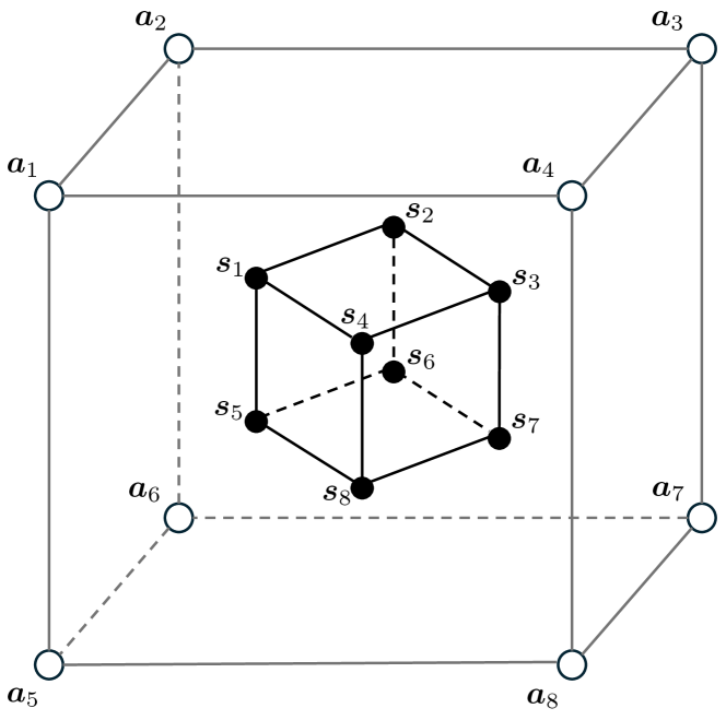
Consider a scenario where a rigid body consisting of $N$ sensors is surrounded by a total of $M$ reference sensors (hereafter referred simply as anchors), as illustrated in Figure 1. Each sensor and anchor is described by a $3\times 1$ vector consisting of its x-,y-,z-coordinates in the 3D Euclidean space, respectively denoted by $\bm{c}_{n}\in\mathbb{R}^{3\times 1}$ for $n=\{1,\ldots,N\}$ and $\bm{a}_{m}\in\mathbb{R}^{3\times 1}$ for $m=\{1,\ldots,M\}$. The initial sensor structure in the rigid body is consequently defined by a conformation matrix $\bm{C}=\left[\bm{c}_{1},\bm{c}_{2},\ldots,\bm{c}_{N}\right]\in\mathbb{R}^{3\times N}$ at the reference frame (local axis) of the rigid body.

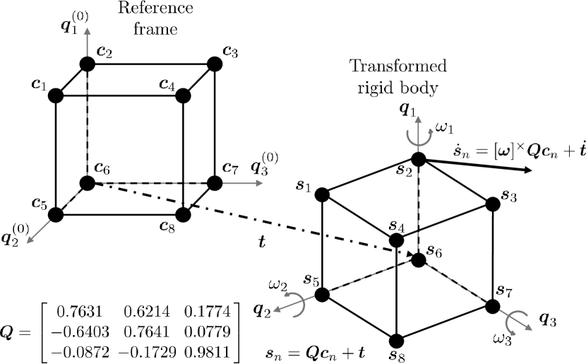
A transformation of the rigid body in 3D space can be fully defined by a translation and rotation, respectively described by the translation vector $\bm{t}\triangleq[t_{x},t_{y},t_{z}]^{\mathsf{T}}\in\mathbb{R}^{3\times 1}$ consisting of the translation distances in each axis, and a 3D rotation matrix111The rotation matrix $\bm{Q}$ is part of the special orthogonal group such that $SO(3)=\left\{\bm{Q}\in\mathbb{R}^{3\times 3}:\bm{Q}^{\mathsf{T}}\bm{Q}=\mathbf{I},~{}\mathrm{det}(\bm{Q})=1\right\}$ [10] . $\bm{Q}\in\mathbb{R}^{3\times 3}$ given by

$\displaystyle\bm{Q}\triangleq\!\text{\scalebox{0.875}{$\overbrace{\left[\begin{array}[]{@{}c@{\;\,}c@{\;\,}c@{}}\cos\theta_{z}&-\sin\theta_{z}&0\\ \sin\theta_{z}&\cos\theta_{z}&0\\ 0&0&1\\ \end{array}\right]}^{\triangleq\,\bm{Q}_{z}\in\,\mathbb{R}^{3\times 3}}\!\cdot\!\overbrace{\left[\begin{array}[]{@{}c@{\;\,}c@{\;\,}c@{}}\cos\theta_{y}&0&\sin\theta_{y}\\ 0&1&0\\ -\sin\theta_{y}&0&\cos\theta_{y}\\ \end{array}\right]}^{\triangleq\,\bm{Q}_{y}\in\,\mathbb{R}^{3\times 3}}\!\cdot\!\overbrace{\left[\begin{array}[]{@{\,}c@{\;\,}c@{\;\,}c@{\!}}1&0&0\\ 0&\cos\theta_{x}&-\sin\theta_{x}\\ 0&\sin\theta_{x}&\cos\theta_{x}\\ \end{array}\right]}^{\triangleq\bm{Q}_{x}\in\,\mathbb{R}^{3\times 3}}$}}\!,$ (10)
Refer to caption
Figure 1: An illustration of the anchor and rigid body sensor structures, in which a cubic rigid body ($N=8$) is surrounded by a cubic deployment of anchors ($M=8$).
Refer to caption
Figure 2: An illustration of a moving rigid body, whose location has a 3D rotation $\bm{Q}$ and a translation $\bm{t}$ from the reference frame333The reference frame is generally not at the origin, but since a rigid body rotation is only relative to its previous orientation, setting the reference frame to the origin, $i.e.$, making $\bm{Q}^{(0)}\triangleq\mathbf{I}_{3\times 3}$, can be done without loss of generality (w.l.g.)., as determined by equation (11). The velocity $\bm{\dot{s}}_{n}$ of the $n$-th sensor as a function of the angular velocity $\bm{\omega}$ and translational velocity $\bm{\dot{t}}$, as determined by equation (12), is also illustrated.

where $\bm{Q}_{x},\,\bm{Q}_{y},\,\bm{Q}_{z}\in\mathbb{R}^{3\times 3}$ are the roll, pitch, and yaw rotation matrices about the x-,y-,z-axes by rotation angles of $\theta_{x},\theta_{y},\theta_{z}\in[-180^{\circ},180^{\circ}]$ degrees, respectively.

In light of the above, the transformed coordinates of the $n$-th sensor after the rotation and translation is described by

$$\bm{s}_{n}=\bm{Q}\bm{c}_{n}+\bm{t}\in\mathbb{R}^{3\times 1},$$ (11)

which is applied identically to all $N$ sensors of the rigid body, as illustrated in Figure 3.

The latter system model for stationary rigid bodies can be extended to moving rigid bodies by introducing the angular velocity vector $\bm{\omega}\triangleq\left[\omega_{1},\omega_{2},\omega_{3}\right]^{\mathsf{T}}\in\mathbb{R}^{3\times 1}$, and the translational velocity vector $\bm{\dot{t}}\triangleq[\dot{t}_{x},\dot{t}_{y},\dot{t}_{z}]^{\mathsf{T}}\in\mathbb{R}^{3\times 1}$, such that the velocity of the $n$-th sensor can be expressed as

$$\dot{\bm{s}}_{n}=[\bm{\omega}]^{\times}\bm{Q}\bm{c}_{n}+\dot{\bm{t}}\in\mathbb{R}^{3\times 1},$$ (12)

where $[\cdot]^{\times}$ is the cross product operator for matrices [10], which maps the angular velocity vector $\bm{\omega}$ to a skew-symmetric matrix, given by

$$[\bm{\omega}]^{\times}=\left[\begin{array}[]{ccc}0&-\omega_{3}&\omega_{2}\\ \omega_{3}&0&-\omega_{1}\\ -\omega_{2}&\omega_{1}&0\end{array}\right]\in\mathbb{R}^{3\times 3}.$$ (13)

II-B Sensor Range Measurement Model

Consider the problem of performing RBL using pairwise range measurements between anchors and sensors, assumed to be available at the anchors, and which are described by

$$\tilde{d}_{m,n}=d_{m,n}+w_{m,n}=\left\|\bm{a}_{m}-\bm{s}_{n}\right\|_{2}+w_{m,n}\in\mathbb{R},$$ (14)

with corresponding squared range measurements modeled as

$$\tilde{d}_{m,n}^{2}=\left\|\bm{a}_{m}-\bm{s}_{n}\right\|_{2}^{2}+2d_{m,n}w_{m,n}+w_{m,n}^{2}\in\mathbb{R}.$$ (15)

In the above, $d_{m,n}\triangleq\left\|\bm{a}_{m}-\bm{s}_{n}\right\|_{2}$ is the true Euclidean distance between the $m$-th anchor and the $n$-th sensor, and $w_{m,n}\sim\mathcal{N}(0,\sigma_{w}^{2})$ is the independent and identically distributed (i.i.d.) additive white Gaussian noise (AWGN) of variance $\sigma_{w}^{2}$ affecting the range measurement, which, following [11, 30, 29], can be reformulated in terms of a linear relation with a composite ranging noise $\xi_{n}\in\mathbb{R}$ given by

$$\xi_{m,n}=\tilde{d}_{m,n}^{2}-\left\|\bm{a}_{m}\right\|^{2}_{2}-\left\|\bm{s}_{n}\right\|^{2}_{2}+2\bm{a}_{m}^{\mathsf{T}}\bm{s}_{n}\approx 2d_{m,n}w_{m,n},$$ (16)

where the second-order noise term $w_{m,n}^{2}$ is neglected.

Stacking equation (16) for all $M$ anchors and reformulating as a linear system on the $n$-th unknown sensor variable yields

$\displaystyle\bm{y}_{n}\!$ $\displaystyle\triangleq\!\!\!\begin{bmatrix}\!\tilde{d}_{1,n}^{2}\!\!-\!\left\|\bm{a}_{1}\right\|^{2}_{2}\!\\ \!\vdots\\ \tilde{d}_{M,n}^{2}\!\!-\!\left\|\bm{a}_{M}\right\|^{2}_{2}\\ \end{bmatrix}\!\!\!=\!\!\!\underbrace{\begin{bmatrix}\!-2\bm{a}_{1}^{\mathsf{T}},&\!\!\!\!1\;\\ \!\vdots&\!\!\!\!\vdots~{}\\ \!-2\bm{a}_{M}^{\mathsf{T}},&\!\!\!\!1\;\\ \end{bmatrix}}_{\triangleq\,\bm{G}\,\in\,\mathbb{R}^{M\!\times\!4}}\!\!\!\!\!\!\!\overbrace{\!\begin{bmatrix}\bm{s}_{n}\\[4.30554pt] ||\bm{s}_{n}||_{2}^{2}\end{bmatrix}\!}^{~{}~{}~{}\triangleq\,\bm{x}_{n}\,\in\,\mathbb{R}^{4\!\times\!1}}\!\!\!\!\!\!+\!\!\!\!\!\!\underbrace{\!\begin{bmatrix}\!\xi_{1,n}\!\\ \!\vdots\!\\ \!\xi_{M,n}\!\\ \end{bmatrix}\!}_{\triangleq\,\bm{\xi}_{n}\,\in\,\mathbb{R}^{M\!\times\!1}}\!\!\!\!\!\!\!\in\!\mathbb{R}^{M\times 1}\!.$

In the latter representation of the observed data vector $\bm{y}_{n}\in\mathbb{R}^{M\times 1}$, we have implicitly defined an effective channel matrix and $\bm{G}$ $\in\mathbb{R}^{M\times 4}$, which is constructed from range measurements and anchor positions; the vector $\bm{x}_{n}\in\mathbb{R}^{4\times 1}$ which contains the unknown coordinates of the $n$-sensor, as well as its distance to the origin; and a vector $\bm{\xi}_{n}\in\mathbb{R}^{M\times 1}$, which gathers the composite noise quantities defined in equation (16).

As hinted in the introduction, the linear system in equation (LABEL:eq:linear_sys) can be leveraged for the estimation of the unknown sensor coordinate vector $\bm{s}_{n}$ and sensor position norm $||\bm{s}||_{2}^{2}$ in $\bm{x}_{n}$, from which equation (11) can be invoked for the translation and rotation extraction via Procrustes analysis or other classical algorithms [9]. We shall return to this idea in Section III.

II-C Sensor Doppler Measurement Model

In addition to the sensor range measurement model relating to the sensor positions, under the assumption of moving rigid bodies and the corresponding sensors, the Doppler measurement information between the anchors and sensors can also be measured, whose relationship is given by

$$\tilde{\nu}_{m,n}=\nu_{m,n}+\epsilon_{m,n}=\frac{\left(\bm{s}_{n}-\bm{a}_{m}\right)^{\mathsf{T}}}{d_{m,n}}\dot{\bm{s}}_{n}+\epsilon_{m,n}\in\mathbb{R},$$ (18)

where ${\nu}_{m,n}\triangleq\frac{\left(\bm{s}_{n}-\bm{a}_{m}\right)^{\mathsf{T}}}{d_{m,n}}\dot{\bm{s}}_{n}\in\mathbb{R}$ is the true Doppler shift between $m$-th anchor and $n$-th sensor, and $\epsilon_{m,n}\sim\mathcal{N}(0,\sigma_{\epsilon}^{2})$ is the i.i.d. AWGN of the Doppler measurement with noise variance $\sigma_{\epsilon}^{2}$.

Multiplying the Doppler measurements of equation (18) with the earlier range measurements of equation (14) yields

$$\tilde{d}_{m,n}\tilde{\nu}_{m,n}\!=\!\bm{s}_{n}^{\mathsf{T}}\dot{\bm{s}}_{n}\!-\!\bm{a}_{m}^{\mathsf{T}}\dot{\bm{s}}_{n}+{\nu}_{m,n}{w}_{m,n}+{d}_{m,n}\epsilon_{m,n}\in\mathbb{R},$$ (19)

which can also be reformulated in terms of a composite Doppler noise $\zeta_{n}\in\mathbb{R}$, given by

$$\zeta_{m,n}\!=\!\tilde{d}_{m,n}\tilde{\nu}_{m,n}\!-\!\bm{s}_{n}^{\mathsf{T}}\dot{\bm{s}}_{n}\!+\!\bm{a}_{m}^{\mathsf{T}}\dot{\bm{s}}_{n}\approx{\nu}_{m,n}{w}_{m,n}\!+\!{d}_{m,n}\epsilon_{m,n}\!\in\!\mathbb{R},$$ (20)

where the second-order noise term $w_{m,n}^{2}$ can be considered negligible [11, 30, 29] and is therefore omitted.

Finally, stacking equation (20) for all $M$ anchors and reformulating as a linear system on the $n$-th unknown sensor variable yields

$\displaystyle\bm{\dot{y}}_{n}\!$ $\displaystyle\triangleq\!\!\!\begin{bmatrix}\!\tilde{d}_{1,n}\tilde{\nu}_{1,n}\\ \!\vdots\\ \tilde{d}_{M,n}\tilde{\nu}_{M,n}\\ \end{bmatrix}\!\!\!=\!\!\!\underbrace{\begin{bmatrix}\!-\bm{a}_{1}^{\mathsf{T}},&\!\!\!\!1\;\\ \!\vdots&\!\!\!\!\vdots~{}\\ \!-\bm{a}_{M}^{\mathsf{T}},&\!\!\!\!1\;\\ \end{bmatrix}}_{\triangleq\,\bm{\dot{G}}\,\in\,\mathbb{R}^{M\!\times\!4}}\!\!\!\!\!\!\!\overbrace{\!\begin{bmatrix}\bm{\dot{s}}_{n}\\[4.30554pt] \bm{s}_{n}^{\mathsf{T}}\bm{\dot{s}}_{n}\end{bmatrix}\!}^{~{}~{}~{}\triangleq\,\bm{\dot{x}}_{n}\,\in\,\mathbb{R}^{4\!\times\!1}}\!\!\!\!\!\!+\!\!\!\!\!\!\underbrace{\!\begin{bmatrix}\!\zeta_{1,n}\!\\ \!\vdots\!\\ \!\zeta_{M,n}\!\\ \end{bmatrix}\!}_{\triangleq\,\bm{\zeta}_{n}\,\in\,\mathbb{R}^{M\!\times\!1}}\!\!\!\!\!\!\!\in\!\mathbb{R}^{M\times 1}\!,$

where $\bm{\dot{y}}_{n}\in\mathbb{R}^{M\times 1}$ and $\bm{\dot{G}}$ $\in\mathbb{R}^{M\times 4}$ are respectively the observed data vector and effective channel matrix constructed from the measured ranges, Doppler shifts and anchor positions, $\bm{\dot{x}}_{n}\in\mathbb{R}^{4\times 1}$ is the unknown sensor velocity vector, and $\bm{\zeta}_{n}\in\mathbb{R}^{M\times 1}$ is the vector of composite noise variables, whose elements are given by equation (20).

The linear system in equation (LABEL:eq:linear_sys_mov) can be leveraged for the estimation of the unknown sensor velocity vector $\bm{\dot{s}}_{n}$ and the multiplication of sensor position and velocity $\bm{s}_{n}^{\mathsf{T}}\bm{\dot{s}}_{n}$ in $\bm{\dot{x}}_{n}$, from which the unknown rigid body transformation variables can be estimated in a similar fashion to the range measurement-based approach in system.

III Proposed Rigid Body Localization

In this section, we propose a low-complexity position and transformation estimator for RBL, in light of the system model derived in Section II and by leveraging the GaBP message passing framework. Specifically, an initial GaBP is derived to solve the position-explicit system in equation (LABEL:eq:linear_sys) to obtain sensor coordinates. Then, in possession of the initial position estimate, a second GaBP is derived on the rigid body transformation parameter-explicit system in equation (28), to obtain the final estimate of the 3D rotation angles $\bm{\theta}$ and translation vector $\bm{t}$.

III-A Stationary Transformation Parameter-based System Model

In this section, we build upon equation (LABEL:eq:linear_sys) towards a reformulation that expresses system variables directly in terms of the RBL transformation parameters, i.e., the 3D rotation angles $\bm{\theta}\triangleq[\theta_{x},\theta_{y},\theta_{z}]^{\mathsf{T}}\in\mathbb{R}^{3\times 1}$ and translation vector $\bm{t}$ [12]. To that end, we first apply a small-angle approximation444For practical rigid body tracking applications, subsequent transformation estimations can be assumed to be performed within a sufficiently short time period, such that the change in rotation angle is small. [10] onto the rotation matrix of equation (10), obtained by leveraging $\cos\theta\approx 1$ and $\sin\theta\approx\theta$, which yields

$\displaystyle~{}~{}~{}~{}\bm{Q}\approx\!\!\left[\begin{array}[]{ccc}1&\theta_{z}&-\theta_{y}\\ -\theta_{z}&1&\theta_{x}\\ \theta_{y}&-\theta_{x}&1\end{array}\right]\in\mathbb{R}^{3\times 3},$ (25)

which in turn can be vectorized into a linear system directly in terms of the Euler angles [11], namely

$\displaystyle\mathrm{vec}(\bm{Q})=\bm{\gamma}+\bm{L}\bm{\theta}=\overbrace{\begin{bmatrix}1&0&0&0&1&0&0&0&1\end{bmatrix}^{\!\mathsf{T}}}^{\triangleq\,\bm{\gamma}\,\in\,\mathbb{R}^{9\times 1}}$ (26)
$\displaystyle+\underbrace{\begin{bmatrix}0&1&0&-1&0&0&0&0&0\\ 0&0&-1&0&0&0&1&0&0\\ 0&0&0&0&0&1&0&-1&0\\ \end{bmatrix}^{\!\mathsf{T}}\!\!\!}_{\triangleq\,\bm{L}\,\in\,\mathbb{R}^{9\times 3}}\cdot\!\begin{bmatrix}\theta_{x}\\ \theta_{y}\\ \theta_{z}\end{bmatrix}\!\!.$

Then substituting equation (26) into equations (11) and (16) and rearranging the terms yields the following alternate representation of the composite noise

$\displaystyle\xi_{n}\!=$ $\displaystyle\tilde{d}_{m,n}^{2}\!-\!\left\|\bm{a}_{m}\right\|^{2}_{2}\!-\!\left\|\bm{s}_{n}\right\|^{2}_{2}\!+\!2\!\left[\bm{c}_{n}^{\mathsf{T}}\otimes\bm{a}_{m}^{\mathsf{T}}\right]\!\bm{\gamma}\!+\!2\!\left[\bm{c}_{n}^{\mathsf{T}}\otimes\bm{a}_{m}^{\mathsf{T}}\right]\!\bm{L}\bm{\theta}$ (27)
$\displaystyle+2\bm{a}_{m}^{\mathsf{T}}\bm{t},\in\mathbb{R},\!\!$

where the matrix product vectorization identity $\mathrm{vec}(\mathbf{XYZ})=(\mathbf{Z}^{\mathsf{T}}\otimes\mathbf{X})\mathrm{vec}(\mathbf{Y})$ has been used, with $\otimes$ denoting the Kronecker product operator.

In light of the above, the fundamental system can be rewritten leveraging the linearization of equation (27),

$$\bm{z}_{n}=\bm{H}_{\theta}\!\cdot\!\bm{\theta}+\bm{H}_{t}\!\cdot\!\bm{t}+\bm{\xi}_{n}\in\mathbb{R}^{M\times 1},$$ (28a)
with
$$\bm{z}_{n}\!=\!\!\left[\!\!\begin{array}[]{c}\tilde{d}_{1,n}^{2}-\left\|\bm{a}_{1}\right\|^{2}_{2}-\left\|\bm{s}_{n}\right\|^{2}_{2}+2\left[\bm{c}_{n}^{\mathsf{T}}\otimes\bm{a}_{1}^{\mathsf{T}}\right]\!\bm{\gamma}\\[4.30554pt] \vdots\\[4.30554pt] \tilde{d}_{M,n}^{2}-\left\|\bm{a}_{M}\right\|^{2}_{2}-\left\|\bm{s}_{n}\right\|^{2}_{2}+2\left[\bm{c}_{n}^{\mathsf{T}}\otimes\bm{a}_{M}^{\mathsf{T}}\right]\!\bm{\gamma}\end{array}\!\!\right]\!\!\in\mathbb{R}^{M\times 1},$$ (28b)
and
$\displaystyle\bm{H}_{\theta}\!=\!\!\left[\begin{array}[]{c}\!\!\!\!\!-2\!\left[\bm{c}_{i}^{\mathsf{T}}\otimes\bm{a}_{1}^{\mathsf{T}}\right]\!\bm{L}\!\!\!\\ \vdots\\[2.15277pt] \!\!\!\!-2\!\left[\bm{c}_{i}^{\mathsf{T}}\otimes\bm{a}_{M}^{\mathsf{T}}\right]\!\bm{L}\!\!\!\end{array}\right]\!\!\in\!\mathbb{R}^{M\times 3}\!,~{}\bm{H}_{t}\!=\!\!\left[\begin{array}[]{c}\!\!\!\!-2\bm{a}_{1}^{\mathsf{T}}\!\!\!\!\\ \vdots\\ \!\!\!\!-2\bm{a}_{M}^{\mathsf{T}}\!\!\!\end{array}\right]\!\!\in\!\mathbb{R}^{M\times 3}\!,$ (28i)

where $\bm{z}_{n}\in\mathbb{R}^{M\times 1}$ is the effective observed data vector, and $\bm{H}_{\theta}\in\mathbb{R}^{M\times 3}$ and $\bm{H}_{t}\in\mathbb{R}^{M\times 3}$ are respectively the effective channel matrices for the unknown rotation and translation variables, and $\bm{\xi}_{n}\in\mathbb{R}^{M\times 1}$ is the vector of composite noise variables from equation (16).

III-B Linear GaBP for Sensor Position Estimation

In what follows, we will derive the step-by-step GaBP message-passing rules for RBL based on the linear model of equation (LABEL:eq:linear_sys). Since the derivation is identical for each $n$-th sensor node, we shall for the sake of convenience temporarily drop the subscript n in the quantities $\bm{y}_{n}$, $\bm{x}_{n}$ and $\bm{\xi}_{n}$ in equation (LABEL:eq:linear_sys), such that we can define the elements of each of these vectors respectively as $\bm{y}_{n}\to\bm{y}=\left[y_{1},\ldots,y_{m},\ldots,y_{M}\right]^{\mathsf{T}},\in\mathbb{R}^{M\times 1}$, $\bm{x}_{n}\to\bm{x}=\left[x_{1},\ldots,x_{k},\ldots,x_{K+1}\right]^{\mathsf{T}},\in\mathbb{R}^{K+1\times 1}$, with $k=\{1,\ldots,K\!+\!1\}$ where $K$ is the dimension of the space, and $\bm{\xi}_{n}\to\bm{\xi}=\left[\xi_{1},\ldots,\xi_{m},\ldots,\xi_{M}\right]^{\mathsf{T}},\in\mathbb{R}^{M\times 1}$. In addition, let $g_{m,k}$ denote the entries of the matrix $\bm{G}$ $\in\mathbb{R}^{M\times K+1}$.

Under such simplified notation, an estimate of the $k$-th element $x_{k}$ of the position vector $\bm{x}$ of a given $n$-th sensor node, from the $m$-th observation $y_{m}$ of the received signal $\bm{y}$ is given by a soft replica denoted by $\hat{x}_{m,k}^{[j]}$, whose mean-squared-error (MSE) is given by

$$\psi_{m,k}^{[j]}=\mathbb{E}_{\mathsf{x}_{k}}\!\!\left\{\big{|}x_{k}-\hat{x}_{m,k}^{[j]}\big{|}^{2}\right\}=\mathbb{E}_{\mathsf{x}_{k}}\!\!\left\{x_{k}^{2}\right\}-\Big{(}\hat{x}_{m,k}^{[j]}\Big{)}^{\!2}\in\mathbb{R},$$ (29)

where the superscript $(\,\cdot\,)^{[j]}$ denotes a quantity at $j$-th iteration of the GaBP.

The first step of GaBP is the soft interference cancellation (soft-IC) on the $m$-th element of the observed data $y_{m}$ for the estimation of the $k$-th estimated variable, described by

$\displaystyle\tilde{y}_{m,k}^{[j]}$ $\displaystyle=y_{m}-\sum_{i\neq k}g_{m,i}\hat{x}_{m,i}^{[j]}$ (30)
$\displaystyle=g_{m,k}x_{k}+\underbrace{\sum_{i\neq k}g_{m,i}\big{(}x_{i}-\hat{x}_{m,i}^{[j]}\big{)}+\xi_{m}}_{\triangleq\,\alpha_{m,k}^{[j]}\,\in\,\mathbb{R}}\in\mathbb{R},$

where $\tilde{y}_{m,k}^{[j]}\in\mathbb{R}$ is the soft-IC symbol corresponding to the $m$-th element of the observed data vector and the $k$-th element of the position vector, and $g_{m,k}\in\mathbb{R}$ is the $(m,k)$-th element of the effective channel matrix $\bm{G}$ in equation (16).

Assuming that the interference-plus-noise term $\alpha_{m,k}^{[j]}\in\mathbb{R}$ in equation (30) follows a normal distribution under the scalar Gaussian approximation [40], the conditional probability density function (PDF) of $\tilde{y}_{x:m,k}^{[j]}$ can be expressed as

$$p_{\tilde{\mathsf{y}}_{m,k}^{[j]}\mid\mathsf{x}_{k}}\!\Big{(}\tilde{y}_{m,k}^{[j]}\big{|}x_{k}\Big{)}\propto\mathrm{exp}\bigg{[}-\frac{\big{|}\tilde{y}_{m,k}^{[j]}-g_{m,k}x_{k}\big{|}^{2}}{\sigma_{m,k}^{2[j]}}\bigg{]}\!,$$ (31)

whose conditional variance is given by

$$\sigma_{m,k}^{2[j]}=\sum_{i\neq k}|g_{m,i}|^{2}\psi_{m,i}^{[j]}+N_{0}\in\mathbb{R},$$ (32)

where $N_{0}$ is the power of the composite noise quantity described in equation (27).

In hand of the conditional PDFs of the soft-IC symbols, the extrinsic PDF of $x_{k}$ can be obtained via

$$\prod_{i\neq m}p_{\tilde{\mathsf{y}}_{i,k}^{[j]}\mid\mathsf{x}_{k}}\!\!\left(\tilde{y}_{i,k}^{[j]}\mid x_{k}\right)\propto\mathrm{exp}\!\bigg{[}-\frac{\big{|}x_{k}-\bar{x}_{m,k}^{[j]}\big{|}^{2}}{\bar{v}_{m,k}^{[j]}}\bigg{]},$$ (33)

with the extrinsic mean and variance respectively given by

$$\bar{x}_{m,k}^{[j]}=\bar{v}_{m,k}^{[j]}\cdot\sum_{i\neq m}\frac{g_{i,k}\!\cdot\!\tilde{y}_{i,k}^{[j]}}{\sigma_{i,k}^{2[j]}}\in\mathbb{R},$$ (34a)
$$\bar{v}_{m,k}^{[j]}=\bigg{(}\sum_{i\neq m}\frac{|g_{i,k}|^{2}}{\sigma_{i,k}^{2[j]}}\bigg{)}^{\!\!-1}\!\!\!\!\!\in\mathbb{R}.$$ (34b)

The extrinsic mean and variance are subsequently denoised with a classic zero-mean Gaussian denoiser555If an alterative prior distribution of the position variables are assumed, i.e., uniform distribution, a different Bayes-optimal denoiser can be utilized., such that the denoised mean and variance are given by

$$\check{x}_{m,k}^{[j]}=\frac{\phi_{x}\bar{x}_{m,k}^{[j]}}{\phi_{x}+\bar{v}_{m,k}^{[j]}}\in\mathbb{R}~{}\,\text{and}\,~{}\check{\psi}_{m,k}^{[j]}=\frac{\phi_{x}\bar{v}_{m,k}^{[j]}}{\phi_{x}+\bar{v}_{m,k}^{[j]}}\in\mathbb{R},\!\!\!$$ (35)

where $\phi_{x}\in\mathbb{R}$ is the variance of the prior distribution of the position variable.

Finally, the $(j\!+\!1)$-th soft-replica is obtained via the following damped update to prevent error floors caused by early erroneous convergence to a local optima

$\displaystyle\hat{x}_{m,k}^{[j+1]}=\rho\hat{x}_{m,k}^{[j]}+(1-\rho)\check{x}_{m,k}^{[j]},$ (36a)
$\displaystyle\psi_{m,k}^{[j+1]}=\rho{\psi}_{m,k}^{[j]}+(1-\rho)\check{\psi}_{m,k}^{[j]},$ (36b)

where $\rho\in[0,1]$ is a selected damping parameter.

Algorithm 1 : Linear GaBP for Position Estimation
1: Input: $\bm{y}_{n}\!~{}\forall n,\;\bm{G},\;\phi_{x},\;N_{0},\;j_{\mathrm{max}},\;\rho$.
2:
3: Output: $\tilde{x}_{k}\!~{}\forall k$ (for all sensor nodes $\forall n$);
4:
5: Perform $\forall n,m,k:$
6:Initialize $\hat{x}_{m,k}^{[1]}$ and $\psi_{m,k}^{[1]}$;
7:for $j=1$ to $j_{\mathrm{max}}$ do
8:      Compute the soft-IC symbol $\tilde{y}_{m,k}^{[j]}$ via eq. (30);
9:      Compute the conditional variance $\sigma_{m,k}^{2[j]}$ via eq. (32);
10:      Compute the extrinsic mean $\bar{x}_{m,k}^{[j]}$ via eq. (34a);
11:      Compute the extrinsic variance $\bar{v}_{m,k}^{[j]}$ via eq. (34b);
12:      Denoise the beliefs $\check{x}_{m,k}^{[j]},\check{\psi}_{m,k}^{[j]}$ via eq. (35);
13:      Update the soft-replicas with damping via eq. (36); $\check{x}_{m,k}^{[j]}$
14:end for
15:Obtain final consensus estimate $\tilde{x}_{k}$ via eq. (37);

At the end of the GaBP iterations, with the last iteration denoted by $j_{\mathrm{max}}$, the final estimate of the position variable is obtained via a consensus belief combination, given by

$$\tilde{x}_{k}=\left(\sum_{m=1}^{M}\frac{|g_{m,k}|^{2}}{\sigma_{m,k}^{2[j_{\mathrm{max}}]}}\right)^{\!\!\!-1}\!\!\!\left(\sum_{m=1}^{M}\frac{g_{m,k}\cdot\tilde{y}_{m,k}^{[j_{\mathrm{max}}]}}{\sigma_{m,k}^{2[j_{\mathrm{max}}]}}\right)\in\mathbb{R}.$$ (37)

Algorithm 1 summarizes the proposed method for the sensor position estimation without rigid body conformation, based on the range information between the sensors and anchors, ultimately yielding $(K+1)$ elements in $\bm{x}_{n}$ composed of $K$ coordinate estimates of $\mathbf{s}_{n}$ and its absolute norm $||\bm{s}_{n}||_{2}^{2}$.

Subsequently, the estimated position information (norm of the sensor coordinate) can be used to construct the second linear equation of equation (28) incorporating the rigid body conformation in terms of the rotation angles and translation vector, as will be leveraged in the following subsection to derive the second GaBP algorithm to directly estimate the rigid body transformation parameters.

III-C Bivariate GaBP for Transformation Parameter Estimation

While the linear formulation and the message passing rules for the GaBP iterations are very similar to Algorithm 1, in the case of transformation parameter estimation based on equation (28), there exist two sets of variables $\theta_{k}$ with $k\in\{1,\ldots,K\}$ and $t_{\ell}$ with $\ell\in\{1,\ldots,K\}$, such that the GaBP rules are elaborated separately. To elaborate, first soft-IC is performed on the observed information respectively for the angle and translation variables as

$\displaystyle\tilde{z}_{\theta:m,k}^{[j]}$ $\displaystyle=z_{m}-\sum_{i\neq k}h_{\theta:m,i}\hat{\theta}_{m,i}^{[j]}-\sum_{i=1}^{K}h_{t:m,i}\hat{t}_{m,i}^{[j]},$ (38a)
$\displaystyle=h_{\theta:m,k}\theta_{k}+\sum_{i=1}^{K}h_{t:m,i}(t_{i}-\hat{t}_{m,i}^{[j]})$
$\displaystyle\hskip 73.19421pt+\sum_{i\neq k}h_{\theta:m,i}(\theta_{i}-\hat{\theta}_{m,i}^{[j]})+\xi_{m},$
$\displaystyle\tilde{z}_{t:m,\ell}^{[j]}$ $\displaystyle=z_{m}-\sum_{i=1}^{K}h_{\theta:m,i}\hat{\theta}_{m,i}^{[j]}-\sum_{i\neq\ell}h_{t:m,i}\hat{t}_{m,i}^{[j]},$ (38b)
$\displaystyle=h_{t:m,\ell}t_{\ell}+\sum_{i=1}^{K}h_{\theta:m,i}(\theta_{i}-\hat{\theta}_{m,i}^{[j]})$
$\displaystyle\hskip 73.19421pt+\sum_{i\neq\ell}h_{t:m,i}(t_{i}-\hat{t}_{m,i}^{[j]})+\xi_{m}.$

In turn, the conditional PDFs of the soft-IC symbols are given by

$\displaystyle p_{\tilde{\mathrm{z}}_{\theta:m,k}^{[j]}\mid\mathrm{\theta}_{k}}(\tilde{z}_{\theta:m,k}^{[j]}|\theta_{k})$ $\displaystyle\propto\mathrm{exp}\bigg{[}-\frac{|\tilde{z}_{\theta:m,k}^{[j]}-h_{\theta:m,k}\theta_{k}|^{2}}{\sigma_{\theta:m,k}^{2\,[j]}}\bigg{]},$ (39)
$\displaystyle p_{\tilde{\mathrm{z}}_{t:m,\ell}^{[j]}\mid\mathrm{t}_{\ell}}(\tilde{z}_{t:m,\ell}^{[j]}|t_{\ell})$ $\displaystyle\propto\mathrm{exp}\bigg{[}-\frac{|\tilde{z}_{t:m,\ell}^{[j]}-h_{t:m,\ell}t_{\ell}|^{2}}{\sigma_{t:m,\ell}^{2\,[j]}}\bigg{]},$

with conditional variances

$$\sigma_{\theta:m,k}^{2\,[j]}\!=\!\displaystyle\sum\limits_{i\neq k}\big{|}h_{\theta:m,i}\big{|}^{2}\psi_{\theta:m,i}^{[j]}\!+\!\sum\limits_{i=1}^{K}\big{|}h_{t:m,i}\big{|}^{2}\psi_{t:m,i}^{[j]}\!+\!N_{0}\in\mathbb{R},$$ (40a)
$$\sigma_{t:m,\ell}^{2\,[j]}\!=\!\displaystyle\sum\limits_{i=1}^{K}\big{|}h_{\theta:m,i}\big{|}^{2}\psi_{\theta:m,i}^{[j]}\!+\!\sum\limits_{i\neq\ell}\big{|}h_{t:m,i}\big{|}^{2}\psi_{t:m,i}^{[j]}\!+\!N_{0}\in\mathbb{R},$$ (40b)
with the corresponding MSEs given by $\psi_{\theta:m,k}^{[j]}=\mathbb{E}_{\mathsf{\theta}_{k}}\!\big{[}|\theta_{k}-\hat{\theta}_{m,k}^{[j]}|^{2}\big{]}$ and $\psi_{t:m,\ell}^{[j]}=\mathbb{E}_{\mathsf{t}_{\ell}}\!\big{[}|t_{\ell}-\hat{t}_{m,\ell}^{[j]}|^{2}\big{]}$, respectively.

With the conditional PDFs in hand, the extrinsic PDF is obtained as

$\displaystyle\prod_{i\neq m}p_{\tilde{\mathsf{z}}_{\theta:i,k}^{[j]}\mid\mathsf{\theta}_{k}}\left(\tilde{z}_{\theta:i,k}^{[j]}\mid\theta_{k}\right)$ $\displaystyle\propto\mathrm{exp}\bigg{[}-\frac{|\theta_{k}-\bar{\theta}_{m,k}^{[j]}|^{2}}{\bar{v}_{\theta:m,k}^{[j]}}\bigg{]},$ (41)
$\displaystyle\prod_{i\neq m}p_{\tilde{\mathsf{z}}_{t:i,\ell}^{[j]}\mid\mathrm{t}_{\ell}}\left(\tilde{z}_{t:i,\ell}^{[j]}\mid t_{\ell}\right)$ $\displaystyle\propto\mathrm{exp}\bigg{[}-\frac{|t_{\ell}-\bar{t}_{m,\ell}^{[j]}|^{2}}{\bar{v}_{t:m,\ell}^{[j]}}\bigg{]},$

where the corresponding extrinsic means and variances are given by

$\displaystyle\bar{\theta}_{m,k}^{[j]}$ $\displaystyle=\bar{v}_{\theta:m,k}^{[j]}\bigg{(}\sum_{i\neq m}\frac{h_{\theta:i,k}\cdot\tilde{z}_{\theta:i,k}^{[j]}}{\big{(}\sigma_{\theta:i,k}^{[j]}\big{)}^{2}}\bigg{)}\in\mathbb{R},$ (42a)
$\displaystyle\bar{t}_{m,\ell}^{[j]}$ $\displaystyle=\bar{v}_{t:m,\ell}^{[j]}\bigg{(}\sum_{i\neq m}\frac{h_{t:i,\ell}\cdot\tilde{z}_{t:i,\ell}^{[j]}}{\big{(}\sigma_{t:i,\ell}^{[j]}\big{)}^{2}}\bigg{)}\in\mathbb{R},$ (42b)
$\displaystyle\bar{v}_{\theta:m,k}^{[j]}$ $\displaystyle=\bigg{(}\sum_{i\neq m}\frac{|h_{\theta:i,k}|^{2}}{\big{(}\sigma_{\theta:i,k}^{[j]}\big{)}^{2}}\bigg{)}^{\!\!\!-1}\!\!\!\!\in\mathbb{R},$ (43a)
$\displaystyle\bar{v}_{t:m,\ell}^{[j]}$ $\displaystyle=\bigg{(}\sum_{i\neq m}\frac{|h_{t:i,\ell}|^{2}}{\sigma_{t:m,\ell}^{2\,[j]}}\bigg{)}^{\!\!\!-1}\!\!\!\!\in\mathbb{R}.$ (43b)

Finally the denoisers with a Gaussian prior are given by

$\displaystyle\check{\theta}_{m,k}$ $\displaystyle=\frac{\phi_{\theta}\cdot\bar{\theta}_{m,k}^{[j]}}{\phi_{\theta}+\bar{v}_{\theta:m,k}^{[j]}}\in\mathbb{R},$ $\displaystyle\check{t}_{m,\ell}$ $\displaystyle=\frac{\phi_{t}\cdot\bar{t}_{m,\ell}^{[j]}}{\phi_{t}+\bar{v}_{t:m,\ell}^{[j]}}\in\mathbb{R},$ (44a)
$\displaystyle\check{\psi}_{\theta:m,k}$ $\displaystyle=\frac{\phi_{\theta}\cdot\bar{v}_{\theta:m,k}^{[j]}}{\phi_{\theta}+\bar{v}_{\theta:m,k}^{[j]}}\in\mathbb{R},$ $\displaystyle\check{\psi}_{t:m,\ell}$ $\displaystyle=\frac{\phi_{t}\cdot\bar{v}_{t:m,\ell}^{[j]}}{\phi_{t}+\bar{v}_{t:m,\ell}^{[j]}}\in\mathbb{R},$ (44b)
where $\phi_{\theta}$ and $\phi_{t}$ are the variance of the elements in $\bm{\theta}$ and $\bm{t}$.
Algorithm 2 : Double GaBP for RBL Parameter Estimation
1: Input: $\bm{z}_{n}\,(||\bm{s}_{n}||_{2}^{2})\!~{}\forall n,\bm{H}_{\theta},\bm{H}_{t},\phi_{\theta},\phi_{t},N_{0},j_{\mathrm{max}},\rho$.
2:
3: Output: $\tilde{\theta}_{k}$ and $\tilde{t}_{\ell}~{}\forall k,\ell$ (for all sensor nodes $\forall n$);
4:
5: Perform $\forall n,m,k,\ell:$
6:Initialise $\hat{\theta}_{m,k}^{[1]}$, $\hat{t}_{m,\ell}^{[1]}$, $\psi_{\theta:m,k}^{[1]}$, $\psi_{t:m,\ell}^{[1]}$;
7:for $j=1$ to $j_{\mathrm{max}}$ do
8:      Compute soft-IC symbols $\tilde{z}_{\theta:m,k}^{[j]}$, $\tilde{z}_{m,\ell}^{t[j]}$ via eq. (38);
9:      Compute conditional variances $\sigma_{\theta:m,k}^{2\,[j]},\sigma_{t:m,\ell}^{2\,[j]}$ via eq. (40);
10:      Compute extrinsic means $\bar{\theta}_{m,k}^{[j]}$, $\bar{t}_{m,\ell}^{[j]}$ via eq. (42);
11:      Compute extrinsic variances $\bar{v}_{\theta:m,k}^{[j]}$, $\bar{v}_{t:m,\ell}^{[j]}$ via eq. (43);
12:      Denoise the beliefs $\check{\theta}_{m,k},\check{t}_{m,\ell}$ via eq. (44a); $\check{x}_{m,k}^{[j]}$
13:      Denoise the error variances $\check{\psi}_{\theta:m,k}\check{\psi}_{t:m,\ell}$ via eq. (44b); $\check{x}_{m,k}^{[j]}$
14:      Update the soft-replicas with damping as in eq. (36); $\check{x}_{m,k}^{[j]}$
15:end for
16:Obtain final consensus estimates $\tilde{\theta}_{k},\tilde{t}_{\ell}$ via eq. (45);
17:Obtain interference-cancelled system via eq. (46);
18:for $j=1$ to $j_{\mathrm{max}}$ do
19:      Compute soft-IC symbols $\tilde{z}{{}^{\prime}}_{\!\!\theta:m,k}^{[j]}$ via eq. (47);
20:      Compute conditional variances $\sigma_{\theta:m,k}^{2\,[j]}$ via eq. (48);
21:      Compute extrinsic means $\bar{\theta}_{m,k}^{[j]}$ via eq. (42a);
22:      Compute extrinsic variances $\bar{v}_{\theta:m,k}^{[j]}$ via eq. (43a);
23:      Denoise the beliefs $\check{\theta}_{m,k}$ via eq. (44a); $\check{x}_{m,k}^{[j]}$
24:      Denoise the error variances $\check{\psi}_{\theta:m,k}$ via eq. (44b); $\check{x}_{m,k}^{[j]}$
25:      Update the soft-replicas with damping as in eq. (36); $\check{x}_{m,k}^{[j]}$
26:end for
27:Obtain refined consensus estimates $\tilde{\theta}_{k}$ via eq. (LABEL:eq:del_t_final_est_theta);

Subsequently, the soft-replicas are iteratively updated similarly to equation (36), with a damping factor $\rho$, for $j_{\mathrm{max}}$ iterations of the message passing algorithm or a convergence criteria, after which the consensus estimates are obtained as

$\displaystyle\tilde{\theta}_{k}$ $\displaystyle=\bigg{(}\sum_{m=1}^{M}\frac{|h_{\theta:m,k}|^{2}}{\big{(}\sigma_{\theta:m,k}^{[j_{\mathrm{max}}]}\big{)}^{2}}\bigg{)}^{\!\!\!-1}\!\!\bigg{(}\sum_{m=1}^{M}\frac{h_{\theta:m,k}\cdot\tilde{z}_{\theta:m,k}^{[j_{\mathrm{max}}]}}{\big{(}\sigma_{\theta:m,k}^{[j_{\mathrm{max}}]}\big{)}^{2}}\bigg{)}\in\mathbb{R},$
$\displaystyle\tilde{t}_{\ell}$ $\displaystyle=\bigg{(}\sum_{m=1}^{M}\frac{|h_{t:m,\ell}|^{2}}{\big{(}\sigma_{t:m,\ell}^{[j_{\mathrm{max}}]}\big{)}^{2}}\bigg{)}^{\!\!\!-1}\!\bigg{(}\sum_{m=1}^{M}\frac{h_{t:m,\ell}\cdot\tilde{z}_{t:m,\ell}^{[j_{\mathrm{max}}]}}{\big{(}\sigma_{t:m,\ell}^{[j_{\mathrm{max}}]}\big{)}^{2}}\,\bigg{)}\in\mathbb{R}.$

While the message passing rules elaborated by equations (38)-(45) are complete to yield the estimated rotation angles and translaction vectors, due to the effective channel powers of $\bm{H}_{\theta}$ and $\bm{H}_{t}$ in equation (28) where the latter is typically much larger absolute positions of the anchors and sensors666The effective channel powers are highly depedent on the sensor and anchor deployment structure, and for typical indoor sensing scenarios as illustrated in Figure 1, the anchor coordinates are of larger absolute value than the rigid body sensor coordinates, leading to the large power difference.. Such significant difference in effective channel powers lead to good estimation performance of the translation vector elements, but erroneous estimation performance of the rotation angles in a joint estimation described by the GaBP procedure.

This behavior can also be intuitively understood by considering the illustration in Figure 3, where a small rotation of the rigid body is expected to have a less prominent effect on the absolute sensor positions then the translation, as assumed in the system formulation of Section II.

In order to address the aforementioned error behavior of the rotation angle parameters $\bm{\theta}$, we propose an interference cancellation-based approach to remove the components corresponding to the translation of the sensors, and perform the GaBP again only on the rotation angle parameters. Namely, by using the estimated consensus translation vector $\tilde{\bm{t}}\triangleq[\tilde{t}_{1},\tilde{t}_{2},\tilde{t}_{3}]^{\mathsf{T}}\!\in\mathbb{R}^{3\times 1}$ obtained at the end of the GaBP via equation (LABEL:eq:del_t_final_est_t), the interference-cancelled system is given by

$$\bm{z}_{n}^{\prime}\triangleq\bm{z}_{n}-\bm{H}_{t}\tilde{\bm{t}}=\bm{H}_{\theta}\bm{\theta}+\bm{\xi}_{n}\in\mathbb{R}^{M\times 1}.\vspace{-1ex}$$ (46)

The GaBP procedure to estimate the rotation angle parameters $\bm{\theta}$ is identical to the linear GaBP of Algorithm 1, except the factor node equations given by

$$\tilde{z}{{}^{\prime}}_{\!\!\theta:m,k}^{[j]}=z^{\prime}_{m}-\sum_{i\neq k}h_{\theta:m,i}\hat{\theta}_{m,i}^{[j]}\in\mathbb{R},\vspace{-1ex}$$ (47)
$$\sigma_{\theta:m,k}^{2\,[j]}=\sum_{i\neq k}\big{|}h_{\theta:m,i}\big{|}^{2}\psi_{\theta:m,i}^{[j]}+N_{0}\in\mathbb{R},\vspace{-1ex}$$ (48)

which is concatenated with the previously described bivariate GaBP to describe the complete estimation process of the rigid body transformation parameters $\bm{\theta}$ and $\bm{t}$, as summarized by Algorithm 2 above.

IV Proposed Rigid Body Motion Estimation

IV-A Velocity Transformation Parameter-based System Model

In this section, following steps similar to those of the reformulation of the system for stationary RBL carried out in the previous section, we reformulate the fundamental system of equation (LABEL:eq:linear_sys_mov) to express in terms of the moving RBL transformation parameters, i.e., the 3D angular velocity $\bm{\omega}\triangleq\left[\omega_{1},\omega_{2},\omega_{3}\right]^{\mathsf{T}}\in\mathbb{R}^{3\times 1}$ and translational velocity vector $\bm{\dot{t}}\in\mathbb{R}^{3\times 1}$ [12], in order to enable their estimation.

Utilizing the same small-angle approximation [10] as before, the angular velocity matrix $[\bm{\omega}]^{\times}$ in equation (13) can be vectorized and decomposed into a linear system directly in terms of the individual velocities [11], yielding

$\displaystyle\mathrm{vec}([\bm{\omega}]^{\times})$ $\displaystyle=\bm{\Phi}\bm{\omega}~{}\in\mathbb{R}^{9\times 1}$ (49)
$\displaystyle=\underbrace{\begin{bmatrix}0&0&0&0&0&1&0&-1&0\\ 0&0&-1&0&0&0&1&0&0\\ 0&1&0&-1&0&0&0&0&0\\ \end{bmatrix}^{\mathsf{T}}\!\!\!}_{\triangleq\,\bm{\Phi}\,\in\,\mathbb{R}^{9\times 3}}\cdot\!\begin{bmatrix}\omega_{1}\\ \omega_{2}\\ \omega_{3}\end{bmatrix}\!\!.$

Then, substituting equation (49) into equations (12) and (20) and rearranging the terms, the following alternate representation of the composite noise is obtained

$\displaystyle\zeta_{m,n}$ $\displaystyle=\tilde{d}_{m,n}\tilde{\nu}_{m,n}-\bm{s}_{n}^{\mathsf{T}}\bm{\dot{s}}_{n}+\bm{a}_{m}^{\mathsf{T}}\left([\bm{\omega}]^{\times}\bm{Q}\bm{c}_{n}+\bm{\dot{t}}\right)$ (50)
$\displaystyle=\tilde{d}_{m,n}\tilde{\nu}_{m,n}-\bm{s}_{n}^{\mathsf{T}}\bm{\dot{s}}_{n}+\left((\bm{Q}\bm{c}_{n})^{\mathsf{T}}\otimes\bm{a}_{m}^{\mathsf{T}}\right)\bm{\Phi}\bm{\omega}+\bm{a}_{m}^{\mathsf{T}}\bm{\dot{t}}\in\mathbb{R},$

where the matrix product vectorization identity $\mathrm{vec}(\mathbf{XYZ})=(\mathbf{Z}^{\mathsf{T}}\otimes\mathbf{X})\mathrm{vec}(\mathbf{Y})$ has been used.

In light of the above, similar as before, the fundamental system can be rewritten leveraging the linearization of equation (50), leading to

$$\bm{u}_{n}\!=\!\!\left[\!\!\begin{array}[]{c}\tilde{d}_{1,n}\tilde{\nu}_{1,n}-\bm{s}_{n}^{\mathsf{T}}\dot{\bm{s}}_{n}\\[-4.30554pt] \vdots\\ \tilde{d}_{M,n}\tilde{\nu}_{M,n}-\bm{s}_{n}^{\mathsf{T}}\dot{\bm{s}}_{n}\end{array}\!\!\right]=\bm{B}_{\omega}\!\cdot\!\bm{\omega}+\bm{B}_{\dot{t}}\!\cdot\!\dot{\bm{t}}+\bm{\zeta}_{n}\in\mathbb{R}^{M\times 1},$$ (51a)
with
$\displaystyle\bm{B}_{\omega}\!\triangleq\!\!\left[\begin{array}[]{c}-\left((\bm{Q}\bm{c}_{n})^{\mathsf{T}}\otimes\bm{a}_{1}^{\mathsf{T}}\right)\bm{\Phi}\\ \vdots\\[2.15277pt] -\left((\bm{Q}\bm{c}_{n})^{\mathsf{T}}\otimes\bm{a}_{M}^{\mathsf{T}}\right)\bm{\Phi}\end{array}\right]\!\!\in\!\mathbb{R}^{M\times 3}\!,$ (51e)
and
$\displaystyle\bm{B}_{\dot{t}}\!\triangleq\!\!\left[\begin{array}[]{c}-\bm{a}_{1}^{\mathsf{T}}\\ \vdots\\ -\bm{a}_{M}^{\mathsf{T}}\end{array}\right]\!\!\in\!\mathbb{R}^{M\times 3}\!,$ (51i)

where $\bm{u}_{n}\in\mathbb{R}^{M\times 1}$ is the effective observed data vector, and $\bm{B}_{\omega}\in\mathbb{R}^{M\times 3}$ and $\bm{B}_{\dot{t}}\in\mathbb{R}^{M\times 3}$ are respectively the effective channel matrices for the unknown angular velocity and translational velocity variables, while $\bm{\zeta}_{n}\in\mathbb{R}^{M\times 1}$ is the vector of composite noise variables from equation (20).

IV-B Linear GaBP for Sensor Velocity Estimation

From the similarity of the structure of the systems in Sections IV-A and Section III-B, it is evident that a linear GaBP can be applied to each $n$-th sensor to form a system of corresponding linear equations. Again, for the sake of notational simplicity, we shall drop subscript n while stressing that the derivations to follow apply to each $n$-th sensor node. To be precise, the estimation of the velocity vector $\bm{\dot{x}}_{n}$ corresponding to any given $n$-th sensor node in equation (LABEL:eq:linear_sys_mov), here temporarily denoted by $\bm{\dot{x}}\triangleq[\dot{x}_{1},\ldots,\dot{x}_{K+1}]^{\mathsf{T}}\in\mathbb{R}^{(K+1)\times 1}$, with $k\in\{1,\ldots,K+1\}$ where $K$ is the dimension of the space, is given by the collection of soft replicas for each of its $k$-th element $\dot{x}_{k}$ for each $m$-th observation, which are denoted by $\hat{\dot{x}}_{m,k}^{[j]}$, whose MSE is defined as

$$\dot{\psi}_{m,k}^{[j]}=\mathbb{E}_{\mathsf{\dot{x}}_{k}}\!\!\left\{\big{|}\dot{x}_{k}-\hat{\dot{x}}_{m,k}^{[j]}\big{|}^{2}\right\}=\mathbb{E}_{\mathsf{\dot{x}}_{k}}\!\!\left\{\dot{x}_{k}^{2}\right\}-\hat{\dot{x}}_{m,k}^{2\,[j]}\in\mathbb{R},$$ (52)

where the superscript $(\,\cdot\,)^{[j]}$ denotes the variable at $j$-th iteration of the GaBP.

First, the soft-IC on the $m$-th element of the observed data $y_{m}$ for the estimation of the $k$-th estimated variable is described by

$\displaystyle\tilde{\dot{y}}_{m,k}^{[j]}$ $\displaystyle=\dot{y}_{m}-\sum_{i\neq k}\dot{g}_{m,i}\hat{\dot{x}}_{m,i}^{[j]}$ (53)
$\displaystyle=\dot{g}_{m,k}\dot{x}_{k}+\underbrace{\sum_{i\neq k}\dot{g}_{m,i}\Big{(}\dot{x}_{i}-\hat{\dot{x}}_{m,i}^{[j]}\Big{)}+\xi_{m}}_{\triangleq\,\beta_{m,k}^{[j]}\,\in\,\mathbb{R}}\in\mathbb{R},$

where $\tilde{\dot{y}}_{m,k}^{[j]}\in\mathbb{R}$ is the soft-IC symbol corresponding to the $m$-th element of the observed data vector and the $k$-th element of the velocity vector and $\dot{g}_{m,k}\in\mathbb{R}$ is the $(m,k)$-th element of the effective channel matrix $\bm{\dot{G}}$ in equation (20).

It can be observed that the GaBP steps are equivalent to the ones presented in Section III-B. In what follows, we shall therefore be brief and described the steps adjusted to the new corresponding linear system of equations succintly.

The conditional PDF of $\tilde{\dot{y}}_{\dot{x}:m,k}^{[j]}$ is given by

$$p_{\tilde{\mathsf{\dot{y}}}_{m,k}^{[j]}\mid\mathsf{\dot{x}}_{k}}\!\Big{(}\tilde{\dot{y}}_{m,k}^{[j]}\big{|}\dot{x}_{k}\Big{)}\propto\mathrm{exp}\!\bigg{[}-\frac{\big{|}\tilde{\dot{y}}_{m,k}^{[j]}-\dot{g}_{m,k}\dot{x}_{k}\big{|}^{2}}{\sigma_{\dot{x}:m,k}^{2[j]}}\bigg{]}\!,$$ (54)

whose conditional variance is given by

$$\sigma_{m,k}^{2[j]}=\sum_{i\neq k}|\dot{g}_{m,i}|^{2}\dot{\psi}_{m,i}^{[j]}+N_{0}\in\mathbb{R},$$ (55)

where $N_{0}$ is the power of the composite noise $\xi_{n}$ described in equation (50).

The extrinsic PDF of $\dot{x}_{k}$ is written as

$$\prod_{i\neq m}p_{\tilde{\mathsf{\dot{y}}}_{i,k}^{[j]}\mid\mathsf{\dot{x}}_{k}}\!\!\left(\tilde{\dot{y}}_{i,k}^{[j]}\mid\dot{x}_{k}\right)\propto\mathrm{exp}\!\bigg{[}-\frac{\big{|}\dot{x}_{k}-\bar{\dot{x}}_{m,k}^{[j]}\big{|}^{2}}{\bar{v}_{m,k}^{[j]}}\bigg{]},$$ (56)

with the extrinsic mean and variance respectively given by

$$\bar{\dot{x}}_{m,k}^{[j]}=\bar{v}_{m,k}^{[j]}\cdot\sum_{i\neq m}\frac{\dot{g}_{i,k}\!\cdot\!\tilde{\dot{y}}_{i,k}^{[j]}}{\sigma_{i,k}^{2[j]}}\in\mathbb{R},$$ (57a)
$$\bar{v}_{m,k}^{[j]}=\bigg{(}\sum_{i\neq m}\frac{|\dot{g}_{i,k}|^{2}}{\sigma_{i,k}^{2[j]}}\bigg{)}^{\!\!-1}\!\!\!\!\!\in\mathbb{R}.$$ (57b)

The denoised mean and variance are given by

$$\check{\dot{x}}_{m,k}^{[j]}=\frac{\phi_{\dot{x}}\bar{\dot{x}}_{m,k}^{[j]}}{\phi_{\dot{x}}+\bar{v}_{m,k}^{[j]}}\in\mathbb{R}~{}\,\text{and}\,~{}\check{\dot{\psi}}_{m,k}^{[j]}=\frac{\phi_{\dot{x}}\bar{v}_{m,k}^{[j]}}{\phi_{\dot{x}}+\bar{v}_{m,k}^{[j]}}\in\mathbb{R}.\!\!\!$$ (58)

The $(j+1)$-th soft-replica is obtained via

$\displaystyle\hat{\dot{x}}_{m,k}^{[j+1]}=\rho\hat{\dot{x}}_{m,k}^{[j]}+(1-\rho)\check{\dot{x}}_{m,k}^{[j]},$ (59a)
$\displaystyle\dot{\psi}_{m,k}^{[j+1]}=\rho{\dot{\psi}}_{m,k}^{[j]}+(1-\rho)\check{\dot{\psi}}_{m,k}^{[j]}.$ (59b)

Finally, the estimate of the position variable is obtained via

$$\tilde{\dot{x}}_{k}=\bigg{(}\sum_{m=1}^{M}\frac{|\dot{g}_{m,k}|^{2}}{\sigma_{m,k}^{2[j_{\mathrm{max}}]}}\bigg{)}^{\!\!\!-1}\!\!\!\bigg{(}\sum_{m=1}^{M}\frac{\dot{g}_{m,k}\cdot\tilde{\dot{y}}_{m,k}^{[j_{\mathrm{max}}]}}{\sigma_{m,k}^{2[j_{\mathrm{max}}]}}\bigg{)}\in\mathbb{R}.\vspace{1ex}$$ (60)

Algorithm 3 summarizes the proposed method for the sensor velocity estimation without rigid body conformation, based on the range information between the sensors and anchors, ultimately yielding $(K+1)$ elements in $\bm{\dot{x}}_{n}$ composed of $K$ velocity estimates of $\mathbf{\dot{s}}_{n}$ and the multiplication of sensor position and velocity $\bm{s}_{n}^{\mathsf{T}}\bm{\dot{s}}_{n}$.

Algorithm 3 : Linear GaBP for Velocity Estimation
1: Input: $\bm{\dot{y}}_{n}\!~{}\forall n,\;\bm{\dot{G}},\;\phi_{\dot{x}},\;N_{0},\;j_{\mathrm{max}},\;\rho$.
2:
3: Output: $\tilde{\dot{x}}_{k}\!~{}\forall k$ (for all sensor nodes $\forall n$);
4:
5: Perform $\forall n,m,k:$
6:Initialize $\hat{\dot{x}}_{m,k}^{[1]}$ and $\dot{\psi}_{m,k}^{[1]}$;
7:for $j=1$ to $j_{\mathrm{max}}$ do
8:      Compute the soft-IC symbol $\tilde{\dot{y}}_{m,k}^{[j]}$ via eq. (53);
9:      Compute the conditional variance $\sigma_{m,k}^{2[j]}$ via eq. (55);
10:      Compute the extrinsic mean $\bar{\dot{x}}_{m,k}^{[j]}$ via eq. (57a);
11:      Compute the extrinsic variance $\bar{v}_{m,k}^{[j]}$ via eq. (57b);
12:      Denoise the beliefs $\check{\dot{x}}_{m,k}^{[j]},\check{\dot{\psi}}_{m,k}^{[j]}$ via eq. (58);
13:      Update the soft-replicas with damping via eq. (59); $\check{\dot{x}}_{m,k}^{[j]}$
14:end for
15:Obtain final consensus estimate $\tilde{\dot{x}}_{k}$ via eq. (60);

Subsequently, the estimated multiplication of sensor position and velocity can be used to construct the second linear equation of equation (51) incorporating the rigid body conformation in terms of the angular velocity and translational velocity, as will be leveraged in the following subsection to derive the second GaBP algorithm to directly estimate the moving rigid body transformation parameters.

IV-C Bivariate GaBP for Velocity Parameter Estimation

Similar to Algorithm 2 of Section III-C, in the case of velocity parameter estimation from equation (51), there exist two sets of variables $\omega_{k}$ with $k\in\{1,\ldots,K\}$ and $\dot{t}_{\ell}$ with $\ell\in\{1,\ldots,K\}$, such that the GaBP rules are elaborated separately. Again, it can be noticed that the individual steps of the GaBP solution are identical to the ones in Section III-C, applied to the new adjusted system model. Thus, the new steps will shortly be summarized hereafter.

The soft-IC for the angular and translational velocity variables is given by

$\displaystyle\tilde{u}_{\omega:m,k}^{[j]}$ $\displaystyle=u_{m}-\sum_{i\neq k}b_{\omega:m,i}\hat{\omega}_{m,i}^{[j]}-\sum_{i=1}^{K}b_{\dot{t}:m,i}\hat{\dot{t}}_{m,i}^{[j]},$ (61a)
$\displaystyle=b_{\omega:m,k}\omega_{k}+\sum_{i=1}^{K}b_{\dot{t}:m,i}(\dot{t}_{i}-\hat{\dot{t}}_{m,i}^{[j]})$
$\displaystyle\hskip 73.19421pt+\sum_{i\neq k}b_{\omega:m,i}(\omega_{i}-\hat{\omega}_{m,i}^{[j]})+\zeta_{m},$
$\displaystyle\tilde{u}_{\dot{t}:m,\ell}^{[j]}$ $\displaystyle=u_{m}-\sum_{i=1}^{K}b_{\omega:m,i}\hat{\omega}_{m,i}^{[j]}-\sum_{i\neq\ell}b_{\dot{t}:m,i}\hat{\dot{t}}_{m,i}^{[j]},$ (61b)
$\displaystyle=b_{\dot{t}:m,\ell}\dot{t}_{\ell}+\sum_{i=1}^{K}b_{\omega:m,i}(\omega_{i}-\hat{\omega}_{m,i}^{[j]})$
$\displaystyle\hskip 64.58313pt+\sum_{i\neq\ell}b_{\dot{t}:m,i}(\dot{t}_{i}-\hat{\dot{t}}_{m,i}^{[j]})+\zeta_{m}.$

In turn, the soft-IC symbol conditional PDFs are given by

$\displaystyle p_{\tilde{\mathrm{u}}_{\omega:m,k}^{[j]}\mid\mathrm{\omega}_{k}}(\tilde{u}_{\omega:m,k}^{[j]}|\omega_{k})$ $\displaystyle\propto\mathrm{exp}\bigg{[}-\frac{|\tilde{u}_{\omega:m,k}^{[j]}-b_{\omega:m,k}\omega_{k}|^{2}}{\sigma_{\omega:m,k}^{2\,[j]}}\bigg{]},$ (62)
$\displaystyle p_{\tilde{\mathrm{u}}_{\dot{t}:m,\ell}^{[j]}\mid\mathrm{\dot{t}}_{\ell}}(\tilde{u}_{\dot{t}:m,\ell}^{[j]}|\dot{t}_{\ell})$ $\displaystyle\propto\mathrm{exp}\bigg{[}-\frac{|\tilde{u}_{\dot{t}:m,\ell}^{[j]}-b_{\dot{t}:m,\ell}\dot{t}_{\ell}|^{2}}{\sigma_{\dot{t}:m,\ell}^{2\,[j]}}\bigg{]},$

with the corresponding conditional variances defined as

$\displaystyle\sigma_{\omega:m,k}^{2\,[j]}$ $\displaystyle=\sum_{i\neq k}\big{|}b_{\omega:m,i}\big{|}^{2}\psi_{\omega:m,i}^{[j]}+\sum_{i=1}^{K}\big{|}b_{\dot{t}:m,i}\big{|}^{2}\psi_{\dot{t}:m,i}^{[j]}+N_{0},$
$\displaystyle\sigma_{\dot{t}:m,\ell}^{2\,[j]}$ $\displaystyle=\sum_{i=1}^{K}\big{|}b_{\omega:m,i}\big{|}^{2}\psi_{\omega:m,i}^{[j]}+\sum_{i\neq\ell}\big{|}b_{\dot{t}:m,i}\big{|}^{2}\psi_{\dot{t}:m,i}^{[j]},$ (63b)
and the corresponding MSEs $\psi_{\omega:m,k}^{[j]}=\mathbb{E}_{\mathsf{\omega}_{k}}\!\big{[}|\omega_{k}-\hat{\omega}_{m,k}^{[j]}|^{2}\big{]}$ and $\psi_{\dot{t}:m,\ell}^{[j]}=\mathbb{E}_{\mathsf{\dot{t}}_{\ell}}\!\big{[}|\dot{t}_{\ell}-\hat{\dot{t}}_{m,\ell}^{[j]}|^{2}\big{]}$.

The extrinsic PDF is obtained as

$\displaystyle\prod_{i\neq m}p_{\tilde{\mathsf{u}}_{\omega:i,k}^{[j]}\mid\mathsf{\omega}_{k}}\left(\tilde{u}_{\omega:i,k}^{[j]}\mid\omega_{k}\right)$ $\displaystyle\propto\mathrm{exp}\bigg{[}-\frac{|\omega_{k}-\bar{\omega}_{m,k}^{[j]}|^{2}}{\bar{v}_{\omega:m,k}^{[j]}}\bigg{]},$ (64)
$\displaystyle\prod_{i\neq m}p_{\tilde{\mathsf{u}}_{\dot{t}:i,\ell}^{[j]}\mid\mathrm{\dot{t}}_{\ell}}\left(\tilde{u}_{\dot{t}:i,\ell}^{[j]}\mid\dot{t}_{\ell}\right)$ $\displaystyle\propto\mathrm{exp}\bigg{[}-\frac{|\dot{t}_{\ell}-\bar{\dot{t}}_{m,\ell}^{[j]}|^{2}}{\bar{v}_{\dot{t}:m,\ell}^{[j]}}\bigg{]},$

where the corresponding extrinsic means and variances are defined to be

$\displaystyle\bar{\omega}_{m,k}^{[j]}$ $\displaystyle=\bar{v}_{\omega:m,k}^{[j]}\bigg{(}\sum_{i\neq m}\frac{b_{\omega:i,k}\cdot\tilde{u}_{\omega:i,k}^{[j]}}{\big{(}\sigma_{\omega:i,k}^{[j]}\big{)}^{2}}\bigg{)}\in\mathbb{R},$ (65a)
$\displaystyle\bar{\dot{t}}_{m,\ell}^{[j]}$ $\displaystyle=\bar{v}_{\dot{t}:m,\ell}^{[j]}\bigg{(}\sum_{i\neq m}\frac{b_{\dot{t}:i,\ell}\cdot\tilde{u}_{\dot{t}:i,\ell}^{[j]}}{\big{(}\sigma_{\dot{t}:i,\ell}^{[j]}\big{)}^{2}}\bigg{)}\in\mathbb{R},$ (65b)
$\displaystyle\bar{v}_{\omega:m,k}^{[j]}$ $\displaystyle=\bigg{(}\sum_{i\neq m}\frac{|b_{\omega:i,k}|^{2}}{\big{(}\sigma_{\omega:i,k}^{[j]}\big{)}^{2}}\bigg{)}^{\!\!\!-1}\!\!\!\!\in\mathbb{R},$ (66a)
$\displaystyle\bar{v}_{\dot{t}:m,\ell}^{[j]}$ $\displaystyle=\bigg{(}\sum_{i\neq m}\frac{|b_{\dot{t}:i,\ell}|^{2}}{\sigma_{\dot{t}:m,\ell}^{2\,[j]}}\bigg{)}^{\!\!\!-1}\!\!\!\!\in\mathbb{R}.$ (66b)

Finally, the denoisers with a Gaussian prior are given by

$\displaystyle\check{\omega}_{m,k}$ $\displaystyle=\frac{\phi_{\omega}\cdot\bar{\omega}_{m,k}^{[j]}}{\phi_{\omega}+\bar{v}_{\omega:m,k}^{[j]}}\in\mathbb{R},$ $\displaystyle\check{\dot{t}}_{m,\ell}$ $\displaystyle=\frac{\phi_{\dot{t}}\cdot\bar{\dot{t}}_{m,\ell}^{[j]}}{\phi_{\dot{t}}+\bar{v}_{\dot{t}:m,\ell}^{[j]}}\in\mathbb{R},$ (67a)
$\displaystyle\check{\psi}_{\omega:m,k}$ $\displaystyle=\frac{\phi_{\omega}\cdot\bar{v}_{\omega:m,k}^{[j]}}{\phi^{\omega}+\bar{v}_{\omega:m,k}^{[j]}}\in\mathbb{R},$ $\displaystyle\check{\psi}_{\dot{t}:m,\ell}$ $\displaystyle=\frac{\phi_{\dot{t}}\cdot\bar{v}_{\dot{t}:m,\ell}^{[j]}}{\phi_{\dot{t}}+\bar{v}_{\dot{t}:m,\ell}^{[j]}}\in\mathbb{R},$ (67b)

where $\phi_{\omega}$ and $\phi_{\dot{t}}$ are the element-wise variances of $\bm{\omega}$ and $\bm{\dot{t}}$.

The $(j+1)$-th soft-replica is obtained via a damped update, described by

$\displaystyle\hat{x}_{m,k}^{[j+1]}=\rho\hat{x}_{m,k}^{[j]}+(1-\rho)\check{x}_{m,k}^{[j]},$ (68a)
$\displaystyle\psi_{m,k}^{[j+1]}=\rho{\psi}_{m,k}^{[j]}+(1-\rho)\check{\psi}_{m,k}^{[j]}.$ (68b)

Finally, after $j_{\mathrm{max}}$ iterations the consensus estimates are obtained from

$\displaystyle\tilde{\omega}_{k}$ $\displaystyle=\bigg{(}\sum_{m=1}^{M}\frac{|b_{\omega:m,k}|^{2}}{\big{(}\sigma_{\omega:m,k}^{[j_{\mathrm{max}}]}\big{)}^{2}}\bigg{)}^{\!\!\!-1}\!\!\bigg{(}\sum_{m=1}^{M}\frac{b_{\omega:m,k}\cdot\tilde{u}_{\omega:m,k}^{[j_{\mathrm{max}}]}}{\big{(}\sigma_{\omega:m,k}^{[j_{\mathrm{max}}]}\big{)}^{2}}\bigg{)}\in\mathbb{R},$
$\displaystyle\tilde{\dot{t}}_{\ell}$ $\displaystyle=\bigg{(}\sum_{m=1}^{M}\frac{|b_{\dot{t}:m,\ell}|^{2}}{\big{(}\sigma_{\dot{t}:m,\ell}^{[j_{\mathrm{max}}]}\big{)}^{2}}\bigg{)}^{\!\!\!-1}\!\bigg{(}\sum_{m=1}^{M}\frac{b_{\dot{t}:m,\ell}\cdot\tilde{u}_{\dot{t}:m,\ell}^{[j_{\mathrm{max}}]}}{\big{(}\sigma_{\dot{t}m,\ell}^{[j_{\mathrm{max}}]}\big{)}^{2}}\,\bigg{)}\in\mathbb{R}.$

Using the estimated consensus translational velocity vector $\tilde{\bm{\dot{t}}}\triangleq[\tilde{\dot{t}}_{1},\tilde{\dot{t}}_{2},\tilde{\dot{t}}_{3}]^{\mathsf{T}}\!\in\mathbb{R}^{3\times 1}$ obtained at the end of the GaBP via equation (LABEL:eq:del_t_final_est_t), the interference-cancelled system is given by

$$\bm{u}_{n}^{\prime}\triangleq\bm{u}_{n}-\bm{B}_{\dot{t}}\tilde{\bm{\dot{t}}}=\bm{B}_{\omega}\bm{\omega}+\bm{\zeta}_{n}\in\mathbb{R}^{M\times 1}.\vspace{-1ex}$$ (70)

The GaBP procedure to estimate the angular velocity parameters $\bm{\omega}$ is identical to the linear GaBP in Algorithm 3, where the post-interference cancellation (IC) factor node equations are given by

$$\tilde{u}{{}^{\prime}}_{\!\!\omega:m,k}^{[j]}=u^{\prime}_{m}-\sum_{i\neq k}b_{\omega:m,i}\hat{\omega}_{m,i}^{[j]}\in\mathbb{R},\vspace{-1ex}$$ (71)
$$\sigma_{\omega:m,k}^{2\,[j]}=\sum_{i\neq k}\big{|}b_{\omega:m,i}\big{|}^{2}\psi_{\omega:m,i}^{[j]}+N_{0}\in\mathbb{R},$$ (72)

which is then again concatenated with the previous bivariate GaBP to describe the complete estimation process for the rigid body transformation parameters $\bm{\omega}$ and $\bm{\dot{t}}$, as summarized by Algorithm 4.

Algorithm 4 : Double GaBP for Moving Rigid Body Motion Parameter Estimation
1: Input: $\bm{u}_{n}\,\bm{s}_{n},\bm{\dot{s}}_{n}\!~{}\forall n,\bm{B}_{\omega},\bm{B}_{\dot{t}},\phi_{\omega},\phi_{\dot{t}},N_{0},j_{\mathrm{max}},\rho$.
2:
3: Output: $\tilde{\omega}_{k}$ and $\tilde{\dot{t}}_{\ell}~{}\forall k,\ell$ (for all sensor nodes $\forall n$);
4:
5: Perform $\forall n,m,k,\ell:$
6:Initialise $\hat{\omega}_{m,k}^{[1]}$, $\hat{\dot{t}}_{m,\ell}^{[1]}$, $\psi_{\omega:m,k}^{[1]}$, $\psi_{\dot{t}:m,\ell}^{[1]}$;
7:for $j=1$ to $j_{\mathrm{max}}$ do
8:      Compute soft-IC symbols $\tilde{u}_{\omega:m,k}^{[j]}$, $\tilde{u}_{\dot{t}:m,\ell}^{[j]}$ via eq. (61);
9:      Compute extrinsic means $\bar{\omega}_{m,k}^{[j]}$, $\bar{\dot{t}}_{m,\ell}^{[j]}$ via eq. (65);
10:      Compute extrinsic variances $\bar{v}_{\omega:m,k}^{[j]}$, $\bar{v}_{\dot{t}:m,\ell}^{[j]}$ via eq. (66);
11:      Denoise the beliefs $\check{\omega}_{m,k},\check{\dot{t}}_{m,\ell}$ via eq. (67a); $\check{x}_{m,k}^{[j]}$
12:      Denoise the error variances $\check{\psi}_{\omega:m,k},\check{\psi}_{\dot{t}:m,\ell}$ via eq. (67b);
13:      Update the soft-replicas with damping as in eq. (68); $\check{x}_{m,k}^{[j]}$
14:end for
15:Obtain final consensus estimates $\tilde{\omega}_{k},\tilde{\dot{t}}_{\ell}$ via eq. (69);
16:Obtain interference-cancelled system via eq. (70);
17:for $j=1$ to $j_{\mathrm{max}}$ do
18:      Compute soft-IC symbols $\tilde{u}{{}^{\prime}}_{\!\!\omega:m,k}^{[j]}$ via eq. (71);
19:      Compute conditional variances $\big{(}\sigma_{\omega:m,k}^{[j]}\big{)}^{2}$ via eq. (72);
20:      Compute extrinsic means $\bar{\omega}_{m,k}^{[j]}$ via eq. (65a);
21:      Compute extrinsic variances $\bar{v}_{\omega:m,k}^{[j]}$ via eq. (66a);
22:      Denoise the beliefs $\check{\omega}_{m,k}$ via eq. (67a); $\check{x}_{m,k}^{[j]}$
23:      Denoise the error variances $\check{\psi}_{\omega:m,k}$ via eq. (67b); $\check{x}_{m,k}^{[j]}$
24:      Update the soft-replicas with damping as in eq. (68); $\check{x}_{m,k}^{[j]}$
25:end for
26:Obtain refined consensus estimates $\tilde{\omega}_{k}$ via eq. (LABEL:eq:omega_t_dot_final_est_theta);

V Performance Analysis

V-A RBL Parameter Estimation Performance Against the SotA

In this section, we present simulation results to demonstrate the effectiveness of the proposed multi-stage GaBP-based approach for RBL. Specifically, we compare the estimation performance of the two stages of the proposed approaches: a) the sensor position estimation via linear GaBP in Algorithm 1, and the RBL transformation parameter estimation via bivariate GaBP and interference cancellation-based refinement GaBP concatenated in Algorithm 2 for a stationary rigid body, and b) the sensor velocity estimation via Algorithm 3, and the RBL velocity parameter estimation via Algorithm 4 for a moving rigid body. The performance is compared against the relevant SotA RBL solution, where the time of arrival (TOA)-based sensor position estimation is performed via the approach in [29], the joint time difference of arrival (TDOA) and frequency difference of arrival (FDOA)-based sensor velocity estimation is performed via the approach in [30] and the RBL parameter estimation is performed via [11].

The simulation setup is the scenario illustrated in Figure 1, where the rigid body is composed of $N=8$ sensors positioned at the vertices of a unit cube at the origin, with sensor positions described by the conformation matrix given by

$$\bm{C}\!=\!\!\leavevmode\resizebox{169.11153pt}{}{$\left[\begin{array}[]{lllllllc}-0.5&\!\phantom{-}0.5&\!\phantom{-}0.5&\!-0.5&\!-0.5&\!\phantom{-}0.5&\!-0.5&\!\phantom{-}0.5\\ -0.5&\!-0.5&\!\phantom{-}0.5&\!\phantom{-}0.5&\!-0.5&\!-0.5&\!\phantom{-}0.5&\!\phantom{-}0.5\\ -0.5&\!-0.5&\!-0.5&\!-0.5&\!\phantom{-}0.5&\!\phantom{-}0.5&\!\phantom{-}0.5&\!\phantom{-}0.5\end{array}\right]$}\!\!\in\!\mathbb{R}^{3\times 8}\!,$$

and the $M=8$ anchors are positioned at the vertices of a larger cube (i.e., room), where the anchor conformation matrix $\bm{A}\in\mathbb{R}^{3\times 8}$ is given by

$$\bm{A}\!=\!\!\leavevmode\resizebox{164.77771pt}{}{$\left[\begin{array}[]{lllllllc}-10&\!\phantom{-}10&\!\phantom{-}10&\!-10&\!-10&\!\phantom{-}10&\!-10&\!\phantom{-}10\\ -10&\!-10&\!\phantom{-}10&\!\phantom{-}10&\!-10&\!-10&\!\phantom{-}10&\!\phantom{-}10\\ -10&\!-10&\!-10&\!-10&\!\phantom{-}10&\!\phantom{-}10&\!\phantom{-}10&\!\phantom{-}10\end{array}\right]$}\!\!\in\!\mathbb{R}^{3\times 8}\!.$$

The RBL rotation angles $\theta_{x},\theta_{y},\theta_{z}$ follow a zero-mean Gaussian distribution of variance $\phi_{\theta}=10$, and the RBL translation vector elements also follow a zero-mean Gaussian distribution of variance $\phi_{t}=5$. The RBL parameters in the moving scenario follow a zero-mean Gaussian distribution of variance $\phi_{\omega}=10$ for the angular velocity and a variance of $\phi_{\dot{t}}=5$ for the translational velocity.

Refer to caption
Figure 3: RMSE of the proposed linear GaBP algorithm for sensor position estimation (Alg. 1) and the SotA method of [29], for various range errors $\sigma$.

The performance is assessed using the RMSE defined as

$$\mathrm{RMSE}=\sqrt{\frac{1}{E}\sum_{i=1}^{E}\|\hat{\bm{x}}^{[i]}-{\bm{x}}\|_{2}^{2}},$$ (73)

where $\hat{\bm{x}}^{[i]}$ is the RBL parameter vector (position, angle, or translation) estimated during the $i$-th Monte-Carlo simulation, $\bm{x}$ is the true RBL parameter vector, and $E=10^{4}$ is the total number of independent Monte-Carlo experiments used for the analysis, and is evaluated for different noise standard deviations $\sigma$ of equation (14) and (18), defined as $\sigma\!=\!\sigma_{w}\!=\!0.1\sigma_{\epsilon}$.

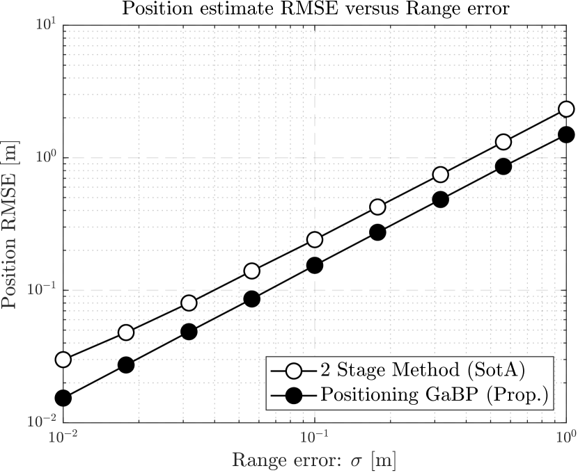
Firstly, for the stationary scenario, Figure 3 illustrates the sensor position estimation performance of the proposed Algorithm 1 and the SotA closed-form solution of [29] for different noise standard deviations, also referred to as range error in meters. It can be observed that the proposed linear GaBP method outperforms the SotA approach for all range error regimes, which suggests that already the proposed preliminary positioning method can be used as an initializer for other SotA methods to perform RBL parameter extraction. In addition, Figures 5 and 5 illustrate the estimation performance of the rigid body translation vector and rotation angles respectively.

Refer to caption
Figure 4: RMSE of the proposed bivariate GaBP algorithm for rigid body translation estimation (Alg. 2) and the SotA method of [11], for various range errors $\sigma$.
Refer to caption
Figure 5: RMSE of the proposed bivariate GaBP algorithm for rigid body rotation angle estimation (Alg. 2) and the SotA method of [11], for various range errors $\sigma$.

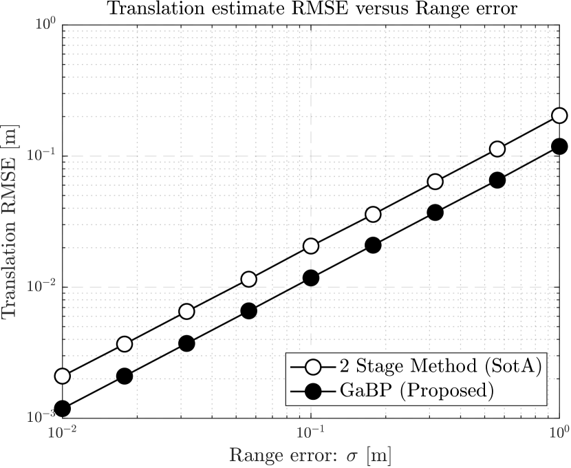
As mentioned in Section III, the translation parameter can be effectively estimated via the proposed bivariate GaBP of Algorithm 2 in light of the channel power difference effect, which is highlighted by the result of Figure 5. It can be seen that the proposed bivariate GaBP algorithm outperforms the SVD-based SotA approach [11] in terms of the rotation angle estimation, for all regimes of range error.

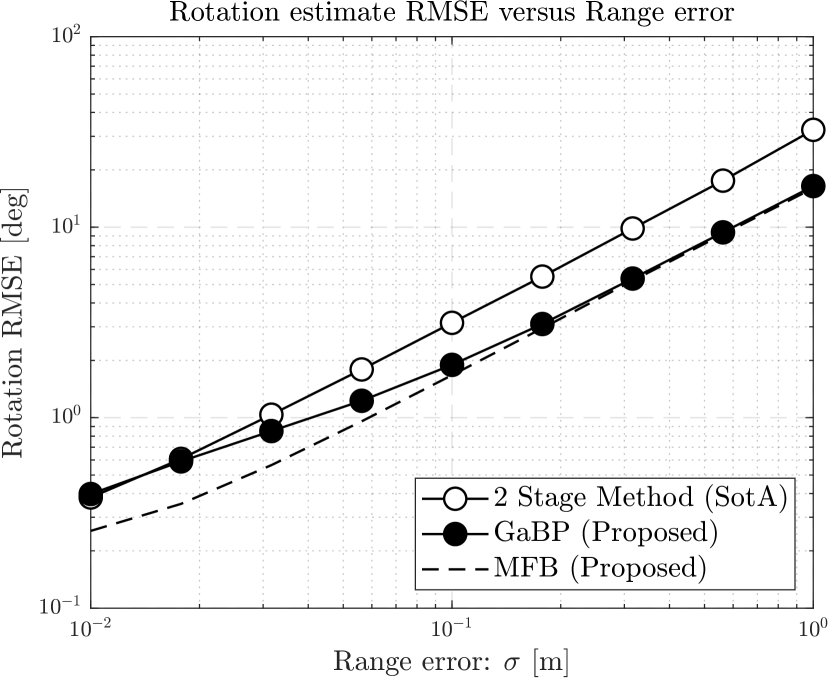
Finally, Figure 5 illustrates the estimation performance of the rotation angles of the rigid body transformation. It can be seen that the estimation performance of the proposed concatenated GaBP also exhibits superiority to the SotA method, similarly to the behavior of the positioning and translation estimation performance. Due to the aforementioned channel power scaling effect which causes the noise power to become more prominent in the estimation of the variables for small range error regimes, the performance of the proposed method can be seen to approach the performance of the SotA in Figure 5. This trend is due to the common error floor usually seen in belief propagation algorithms at smaller error regions, which can be further optimized via procedures such as adaptive damping [41].

Additionally, the ideal behavior of the proposed algorithm is illustrated via the matched filter bound (MFB) of the GaBP algorithm, which shows the expected superiority over all noise ranges, also illustrating that for high noise, the proposed method indeed reaches the optimal performance.

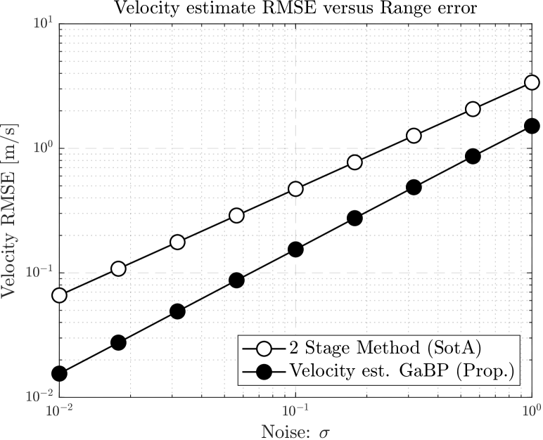
Next, the second set of results evaluates the performance of the proposed rigid body motion estimation algorithms within the moving rigid body scenario. First, Figure 7 illustrates the RMSE of the sensor velocity estimates of Algorithm 3 compared to the SotA solution of [30]. It can be observed that the proposed method outperforms the SotA in all velocity errors with a large performance gain.

Refer to caption
Figure 6: RMSE of the proposed linear GaBP algorithm for sensor velocity estimation (Alg. 3) and the SotA method of [30], for various noise levels $\sigma$.
Refer to caption
Figure 7: RMSE of the proposed bivariate GaBP algorithm for rigid body translational velocity estimation (Alg. 4) and the SotA method of [11], for various noise levels $\sigma$.
Refer to caption
Figure 8: RMSE of the proposed bivariate GaBP algorithm for rigid body angular velocity estimation (Alg. 4) and the SotA method of [11], for various noise levels $\sigma$.

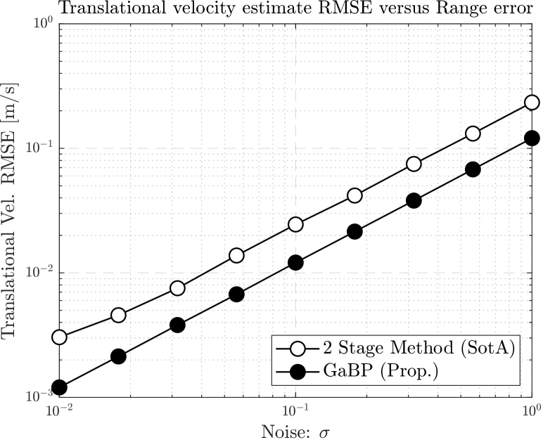
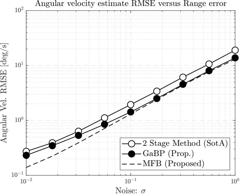
Finally, Figures 7 and 8 show the performance of the estimate velocity parameters, $i.e.$, the angular velocity and the translational velocity. In Figure 7, the translational velocity estimate of the proposed method in Algorithm 4 is compared to the SotA method of [11]. It can be observed that as previously, the proposed method outperforms the SotA for all range errors. In turn, Figure 8 illustrates the performance of the angular velocity estimation, where similar to the stationary rotation estimation results, the proposed method outperforms the SotA for all range errors, with a larger gain reaching the MFB for high noise and a smaller gain for low noise.

V-B Convergence Behavior and Complexity Analysis

Here, the performance of the proposed RBL parameter estimation algorithms are further assessed in terms of the computational complexity and convergence behavior, which is thoroughly investigated in [42, 43, 44], and compared against the SotA methods.

Refer to caption
Figure 9: Convergence of the proposed algorithms for a noise level of $\sigma=10^{-1}$.
TABLE I: Complexity and Runtime
Method Complexity Runtime
Prop. Stationary Linear GaBP (Alg. 1) $O(NMK)$ $0.15$ms
Prop. Moving Linear GaBP (Alg. 3) $O(NMK)$ $0.14$ms
SotA Position/Velocity Est. [30] $O(MNK^{2})$ $1.6$ms
Prop. Stationary Double GaBP (Alg. 2) $O(NMK^{2})$ $1.1$ms
SotA Stationary Parameter Est. [11] $O(K^{3}+MN)$ $0.24$ms
Prop. Moving Double GaBP (Alg. 4) $O(NMK^{2})$ $1$ms
SotA Moving Parameter Est. [11] $O(K^{3}+MN)$ $0.39$ms

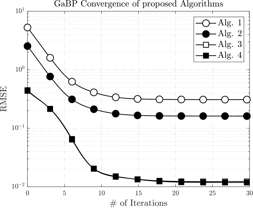
First, Figure 9 illustrates the convergence behaviour of the four proposed algorithms, where it can be observed that all four algorithms converge very efficiently, with the bivariate Algorithm 1 and 3 converging slightly faster and to a higher estimation accuracy than the two linear algorithms. It should also be noted that since the SotA algorithms are not iterative, a convergence analysis comparison is not relevant.

Finally, the computational complexities of the proposed algorithms have been outlined in Table I in terms of the complexity order on the system size parameters using the well-known Big-O notation, as well as a convenient measure of practical runtimes in seconds simulated via an ordinary computer.

VI Conclusion

We presented a novel and efficient framework for solving the sixth-dimensional (6D) RBL problem, for under stationary and moving i.e., estimation of 3D location and 3D rotation, as well as corresponding translation and angular velocities, via a series of tailored GaBP message passing estimators. First, a linear GaBP for the sensor position estimation based on the obtained range estimates from the wireless sensors is derived, from which the RBL system is reformulated via the small-angle approximation to enable the construction of a second bivariate GaBP which is capable of directly estimating the rotation angles and the translation distances. Next, Doppler measurements were obtained, designing a system of linear equations that can be used to estimate the sensor velocity via a linear GaBP, followed by the estimation of angular and translational velocity by the construction of another bivariate GaBP. The proposed RBL method is shown to outperform the SotA method in all of the position, rotation, translation, sensor velocity, angular velocity and translational velocity estimation performance, in addition to the complexity advantage highlighted by the analysis.

References

  • [1] V. Vizitiv, H. S. Rou, N. Führling, and G. T. F. de Abreu, ”Belief Propagation-based Rotation and Translation Estimation for Rigid Body Localization,” arXiv preprint arXiv:2407.09232, 2024.
  • [2] M. A. Jamshed, K. Ali, Q. H. Abbasi, M. A. Imran, and M. Ur-Rehman, “Challenges, Applications, and Future of Wireless Sensors in Internet of Things: A Review,” IEEE Sensors Journal, vol. 22, no. 6, pp. 5482–5494, 2022.
  • [3] D. Kandris, C. Nakas, D. Vomvas, and G. Koulouras, “Applications of Wireless Sensor Networks: An Up-to-Date Survey,” Applied System Innovation, vol. 3, no. 1, p. 14, 2020.
  • [4] J. Lee, S. C. Ahn, and J.-I. Hwang, “A Walking-in-Place Method for Virtual Reality using Position and Orientation Tracking,” Sensors, vol. 18, no. 9, p. 2832, 2018.
  • [5] N. Patwari, J. Ash, S. Kyperountas, A. Hero, R. Moses, and N. Correal, “Locating the Nodes: Cooperative Localization in Wireless Sensor Networks,” IEEE Signal Processing Magazine, vol. 22, no. 4, pp. 54–69, 2005.
  • [6] F. Gustafsson and F. Gunnarsson, “Mobile Positioning using Wireless Networks: Possibilities and Fundamental Limitations Based on Available Wireless Network Measurements,” IEEE Signal Processing Magazine, vol. 22, no. 4, pp. 41–53, 2005.
  • [7] T.-L. Yang, A.-X. Liu, Q. Jin, Y.-F. Luo, H.-P. Shen, and L.-B. Hang, “Position and Orientation Characteristic Equation for Topological Design of Robot Mechanisms,” Journal of Mechanical Design, vol. 131, no. 2, p. 021001, 2008.
  • [8] W. Whittaker and L. Nastro, “Utilization of Position and Orientation Data for Preplanning and Real Time Autonomous Vehicle Navigation,” in IEEE/ION Position, Location, And Navigation Symposium, 2006.
  • [9] D. W. Eggert, A. Lorusso, and R. B. Fisher, “Estimating 3-D Rigid Body Transformations: A Comparison of Four Major Algorithms,” Machine Vision and Applications, vol. 9, no. 5, pp. 272–290, 1997.
  • [10] J. Diebel, “Representing Attitude: Euler Angles, Unit Quaternions, and Rotation Vectors,” Matrix, vol. 58, no. 15-16, pp. 1–35, 2006.
  • [11] S. Chen and K. C. Ho, “Accurate Localization of a Rigid Body Using Multiple Sensors and Landmarks,” IEEE Transactions on Signal Processing, vol. 63, no. 24, pp. 6459–6472, 2015.
  • [12] L. Zha, D. Chen, and G. Yang, “3D Moving Rigid Body Localization in the Presence of Anchor Position Errors,” 2021.
  • [13] Q. Yu, Y. Wang, Y. Shen, and X. Shi, “Cooperative Multi-Rigid-Body Localization in Wireless Sensor Networks Using Range and Doppler Measurements,” IEEE Internet of Things Journal, 2023.
  • [14] N. Führling, H. S. Rou, G. T. F. de Abreu, D. G. G., and O. Gonsa, “Enabling Next-Generation V2X Perception: Wireless Rigid Body Localization and Tracking,” 2024. [Online]. Available: https://arxiv.org/abs/2408.00349
  • [15] W. Chaoyi, Y. Hua, T. Song, Z. Xue, R. Ma, N. Robertson, and H. Guan, “Fine-Grained Pose Temporal Memory Module for Video Pose Estimation and Tracking,” in IEEE International Conference on Acoustics, Speech and Signal Processing (ICASSP).   IEEE, 2021.
  • [16] Y. Xiang, T. Schmidt, V. Narayanan, and D. Fox, “PoseCNN: A Convolutional Neural Network for 6D Object Pose Estimation in Cluttered Scenes,” arXiv preprint arXiv:1711.00199, 2017.
  • [17] F. Aghili and A. Salerno, “Driftless 3-D Attitude Determination and Positioning of Mobile Robots By Integration of IMU With Two RTK GPSs,” IEEE/ASME Transactions on Mechatronics, vol. 18, no. 1, pp. 21–31, 2013.
  • [18] J. Zhao, “A Review of Wearable IMU (inertial-measurement-unit)-based Pose Estimation and Drift Reduction Technologies,” in Journal of Physics: Conference Series, vol. 1087.   IOP Publishing, 2018.
  • [19] A. Alcocer, P. Oliveira, A. Pascoal, R. Cunha, and C. Silvestre, “A Dynamic Estimator on SE(3) using Range-Only Measurements,” in IEEE Conference on Decision and Control, 2008.
  • [20] S. Sand, A. Dammann, and C. Mensing, Positioning in Wireless Communications Systems, 1st ed.   Wiley Publishing, 2014.
  • [21] A. Pizzo, S. P. Chepuri, and G. Leus, “Towards Multi-Rigid Body Localization,” in IEEE International Conference on Acoustics, Speech and Signal Processing (ICASSP), 2016.
  • [22] J. Jiang, G. Wang, and K. C. Ho, “Accurate Rigid Body Localization via Semidefinite Relaxation Using Range Measurements,” IEEE Signal Processing Letters, vol. 25, no. 3, pp. 378–382, 2018.
  • [23] G. Wang and K. C. Ho, “Accurate Semidefinite Relaxation Method for 3-D Rigid Body Localization using AOA,” in IEEE International Conference on Acoustics, Speech and Signal Processing (ICASSP), 2020.
  • [24] S. P. Chepuri, G. Leus, and A.-J. van der Veen, “Rigid Body Localization Using Sensor Networks,” IEEE Transactions on Signal Processing, vol. 62, no. 18, pp. 4911–4924, 2014.
  • [25] B. Zhou, L. Ai, X. Dong, and L. Yang, “DOA-based Rigid Body Localization Adopting Single Base Station,” IEEE Communications Letters, vol. 23, no. 3, pp. 494–497, 2019.
  • [26] Y. Wang, G. Wang, S. Chen, K. C. Ho, and L. Huang, “An Investigation and Solution of Angle Based Rigid Body Localization,” IEEE Transactions on Signal Processing, vol. 68, pp. 5457–5472, 2020.
  • [27] Q. Yu, Y. Wang, Y. Shen, and X. Shi, “Cooperative Multi-Rigid-Body Localization in Wireless Sensor Networks using Range and Doppler Measurements,” IEEE Internet of Things Journal, vol. 10, no. 24, pp. 22 748–22 763, 2023.
  • [28] J. Jiang, G. Wang, and K. C. Ho, “Sensor Network-based Rigid Body Localization via Semi-Definite Relaxation using Arrival Time and Doppler Measurements,” IEEE Transactions on Wireless Communications, vol. 18, no. 2, pp. 1011–1025, 2019.
  • [29] Z. Ma and K. Ho, “TOA Localization in the Presence of Random Sensor Position Errors,” in IEEE International Conference on Acoustics, Speech and Signal Processing (ICASSP), 2011.
  • [30] K. Ho and W. Xu, “An Accurate Algebraic Solution for Moving Source Location using TDOA and FDOA Measurements,” IEEE Transactions on Signal Processing, vol. 52, no. 9, pp. 2453–2463, 2004.
  • [31] T. Vaskevicius and N. Zhivotovskiy, “Suboptimality of Constrained Least Squares and Improvements via Non-Linear Predictors,” Bernoulli, 2023.
  • [32] O. Y. Feng, R. Venkataramanan, C. Rush, and R. J. Samworth, A Unifying Tutorial on Approximate Message Passing, ser. Foundations and Trends in Communications and Information Theory.   Now Publishers Inc, Jun. 28 2022.
  • [33] X. Zhu, Y. Ma, X. Li, and T. Li, “Alternating Subspace Approximate Message Passing,” 2024. [Online]. Available: https://arxiv.org/abs/2407.07436
  • [34] J. T. Parker, P. Schniter, and V. Cevher, “Bilinear Generalized Approximate Message Passing—Part I: Derivation,” IEEE Transactions on Signal Processing, vol. 62, no. 22, pp. 5839–5853, 2014.
  • [35] ——, “Bilinear Generalized Approximate Message Passing—Part II: Applications,” IEEE Transactions on Signal Processing, vol. 62, no. 22, pp. 5854–5867, 2014.
  • [36] T. Takahashi, H. Iimori, K. Ando, K. Ishibashi, S. Ibi, and G. T. F. de Abreu, “Bayesian Receiver Design via Bilinear Inference for Cell-Free Massive MIMO with Low-Resolution ADCs,” IEEE Transactions on Wireless Communications, vol. 22, no. 7, pp. 4756–4772, 2023.
  • [37] W. Yuan, N. Wu, B. Etzlinger, H. Wang, and J. Kuang, ”Cooperative Joint Localization and Clock Synchronization Based on Gaussian Message Passing in Asynchronous Wireless Networks,” IEEE Transactions on Vehicular Technology, vol. 65, no. 9, pp. 7258–7273, 2016.
  • [38] D. Jin, F. Yin, C. Fritsche, F. Gustafsson, and A. M. Zoubir, ”Bayesian Cooperative Localization Using Received Signal Strength With Unknown Path Loss Exponent: Message Passing Approaches,” IEEE Transactions on Signal Processing, vol. 68, pp. 1120–1135, 2020.
  • [39] Z. Yu, J. Li, Q. Guo, and J. Ding, ”Efficient Direct Target Localization for Distributed MIMO Radar With Expectation Propagation and Belief Propagation,” IEEE Transactions on Signal Processing, vol. 69, pp. 4055–4068, 2021.
  • [40] A. Chockalingam and B. S. Rajan, Large MIMO Systems.   Cambridge University Press, 2014.
  • [41] J. Vila, P. Schniter, S. Rangan, F. Krzakala, and L. Zdeborová, “Adaptive Damping and Mean Removal for the Generalized Approximate Message Passing Algorithm,” in IEEE International Conference on Acoustics, Speech and Signal Processing (ICASSP), 2015.
  • [42] Q. Su and Y.-C. Wu, ”Convergence Analysis of the Variance in Gaussian Belief Propagation,” IEEE Transactions on Signal Processing, vol. 62, no. 19, pp. 5119–5131, 2014.
  • [43] Q. Su and Y.-C. Wu, ”On Convergence Conditions of Gaussian Belief Propagation,” IEEE Transactions on Signal Processing, vol. 63, no. 5, pp. 1144–1155, 2015.
  • [44] B. Li, Q. Su, and Y.-C. Wu, ”Fixed Points of Gaussian Belief Propagation and Relation to Convergence,” IEEE Transactions on Signal Processing, vol. 67, no. 23, pp. 6025–6038, 2019.