Quantum sampling on a quantum annealer for large volumes in the strong coupling limit for gauge group U(3)

Abstract

In our previous studies [1, 2], we confirmed that a quantum annealer can be used for importance sampling of gauge theories. In this paper, we extend the previous results to larger 2-dimensional and 4-dimensional lattices to generate ensembles for ${\rm U}(3)$ gauge theory in the strong coupling limit. We make use of the D-Wave quantum annealer to generate histograms for sub-lattices, and use the Metropolis-Hastings algorithm to determine thermodynamic observables and their dependence on the physical parameters on large volumes. We benchmark our results to those obtained from classical Monte Carlo simulations.

I Introduction

Quantum annealers are promising devices for ensemble generation in statistical physics and field theory. The examples of quantum sampling range from boson sampling [3] to sampling proteins [4]. Also, many different methods are on the market for quantum annealers: the noisy Gibbs sampler [5], methods to investigate phase transition [6], hybrid approach [7], and the annealer as a quantum thermal sampler [8]. Quantum sampling of statistical ensembles requires however an additional step to obtain ensembles according to the target equilibrium distribution that depends on the physical parameters of the investigated theory [9, 10, 11]. On a classical computer, via a Monte Carlo, importance sampling is realized e.g. by the Metropolis algorithm. In our effective theory, which is governed by a constraint on admissible configurations, ensemble generation is a difficult task, specifically at low temperature. In contrast, on a quantum annealer, the admissible configurations can be generated easily with the so-called QUBO formalism which is independent of the temperature.

The scope of this paper is to address larger volumes compared to our previous studies [1, 2]. We use the D-wave advantage system that has the Pegasus topology [12] and consists of 5600 physical qubits. This system can only accommodate small lattice volumes. Large volumes, on the other hand, require an alternative scheme that can sample smaller sub-volumes, or sub-lattices. The central idea of our work is to make use of an iterative scheme that embeds sub-lattices in parallel with specific boundaries that are fixed by the previous quantum sampling step. This scheme ultimately allows us to generate larger volume configurations.

After short introduction about the effective theory in Sec. II, we explain the technical aspects to address large volumes in Sec. III. We present our results on the volume and parameter dependence of observables in Sec. IV.

II Effective theory of Lattice QCD

Our effective theory is derived from staggered fermions in the strong coupling limit, which is well known to have a dual representation in terms of integer-valued dual variables [13]. These dual variables consist of so-called monomers $m(n)$ and dimers $d_{\nu}(n)$ (with $n$ a lattice coordinate) for ${\rm U}(3)$ gauge theory, and also baryonic world-lines, which have to be included for ${\rm SU}(3)$ gauge theory. We have studied ${\rm SU}(3)$ in [2] but in this work we restrict ourselves to ${\rm U}(3)$ for simplicity. As explained detail in [1], the integer-valued dual variables can be mapped to a binary vector $x$ which can be adapted for the quadratic unconstrained binary optimization (QUBO) formalism:

$$\chi^{2} =x^{T}Qx\,,$$

$$Q =W+p(A^{T}A+diag(2b\cdot A))\,.$$ (1)

Here $Q$ is the quadratic QUBO matrix generated by the weight matrix $W$ that is determined from the effective action, as well as $A$ that incorporates the constraints that stem from the Grassmann integration of the quarks. The penalty factor $p$ favors ($p\gg 1$) or disfavors ($p\ll 1$) the constraint over the weight matrix. As we explain in more detail in the next section, we embed in parallel $2\times 2$ sub-lattices such that for each sub-lattice different boundaries $b$ are applied. More precisely, the weight matrix of $Q$ is determined for ${\rm U}(3)$ gauge group via

$$M =\left(\begin{array}[]{cc}-2\log(2m_{q})+\log(2)&\log(3)\\ 0&-\log(2m_{q})\\ \end{array}\right)$$ (4)

$$D_{s} =\left(\begin{array}[]{cc}\log(12)&0\\ 0&\log(3)\\ \end{array}\right)$$ (7)

$$D_{t} =\left(\begin{array}[]{cc}\log(12)-4\log(\gamma)&0\\ 0&\log(3)-2\log(\gamma)]\\ \end{array}\right)$$ (10)

$$W =diag(M,M,M,M,D_{s},D_{s},D_{t},D_{t})$$ (11)

and the constraint and boundary are given by

$$A =\left(\begin{array}[]{cccccccccccccccc}2&1&0&0&0&0&0&0&2&1&0&0&2&1&0&0\\ 0&0&2&1&0&0&0&0&2&1&0&0&0&0&2&1\\ 0&0&0&0&2&1&0&0&0&0&2&1&2&1&0&0\\ 0&0&0&0&0&0&2&1&0&0&2&1&0&0&2&1\\ \end{array}\right)$$ (16)

$$b =(3-d_{ext}^{(1)},3-d_{ext}^{(2)},3-d_{ext}^{(3)},3-d_{ext}^{(4)})\,,$$ (17)

where $d_{ext}^{(x)}$ corresponds to the number of external dimers. This quantity changes after each update as explained in Sec. III.1.

III Technical development

In order to sample our effective theory on D-wave, we have to map logical qubit $x$ as in Eq. II to the physical qubits with connectivities given by the Pegasus topology. This can be achieved by synchronized combination of physical qubits (”chain”) to form a logical qubit, as discussed in detail in [1]. With 5600 physical qubits available, only small volumes can be sampled at once.

For larger volumes, we use an iterative scheme that only samples disconnected sub-lattices, keeping dimers that are not part of the sub-lattice fixed, see Eq. 17. An example of the decomposition to sub-lattices is given in Fig. 1. Only the degrees of freedom inside the red boxes are sampled, and this is done in parallel to maximize the use of qubits.

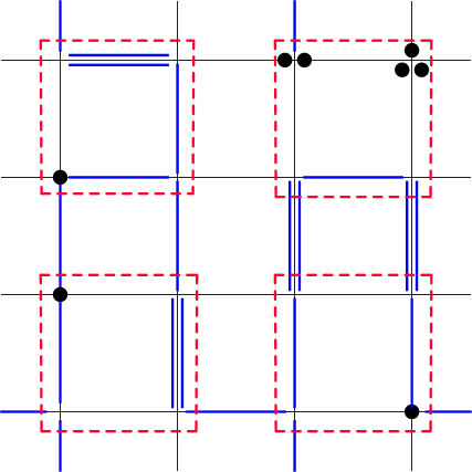
Figure 1: Selecting $2\times 2$ sub volume with fixed boundary condition. Black dots are monomers, blue lines are dimers. Monomers and dimers inside of red boxes are updated in parallel. The Grassmann constraint is required to be satisfied at each site.

III.1 Parallel Sampling scheme

In order to sample all degrees of freedom, we scan all possible sub-lattices, defined by the base point and all directions to span the volume by the sub-lattices, as shown in Table 1.

V	$V_{\text{sub}}$	ind. sub-lat.	base points
$4\times 4$	$2\times 2$	4	4
$8\times 8$	$2\times 2$	16	4
$16\times 16$	$2\times 2$	64	4
$32\times 32$	$2\times 2$	256	4
$4\times 4\times 4$	$2\times 2$	16	12
	$2\times 2\times 2$	8	8
$4\times 4\times 4\times 4$	$2\times 2$	64	24
	$2\times 2\times 2$	32	32
$8\times 8\times 8\times 4$	$2\times 2$	512	24
	$2\times 2\times 2$	256	32

Table 1: Parallelization by sub-lattice sampling. # of ind. sub-lattices corresponds to the number of sub-lattices sampled in parallel. # of base points is the number of sites in sub-lattice. For one volume sweep, it is required to sample sub-lattices in parallel for every base point.

We choose the sub-lattices of size $2\times 2$ (square sampling), and of size $2\times 2\times 2$ (cube sampling). Clearly, the sub-lattice dimension $d_{s}$ has to be smaller or equal to the dimension $d$ of the lattice volume. For $d_{s}<d$, we have to loop through $\binom{d}{d_{s}}$ sets of directions to sample the full volume. For $2\times 2$ sub-lattices, 16 logical qubits are required per sub-lattice and for $2\times 2\times 2$ sub-lattice, 40 logical qubits. Since the number of sub-lattices is $V/V_{sub}$, the number of logical qubits for lattice size $V=N_{s}^{(d-1)}\times N_{t}$ is $2V(1+d/2)$ with $d$ the dimension of the volume. If the lattice is too large, we choose randomly a maximal subset of sub-lattices ($2\times 2$: 170, $2\times 2\times 2$: 45) to sample in parallel. This results in a block-diagonal form of the QUBO matrix $Q$. The quantum annealer then solves for $x$ in a fixed amount of time regardless of how many qubits are used in the parallelization.

It is sufficient to sample every degree of freedom by sequentially going through all base points that define the location of sub-lattice. The number of base points on a $d$-dimensional lattice is obtained by the binomial coefficient

$$V_{sub}\times\binom{d}{d_{s}}\,.$$ (18)

The solution vector for a new base point depends on the previous solution vector because the fixed boundary $b$ ($d^{(x)}_{ext}$) in Eq. (17) changes after each update. For the square sampling, we have $({N_{c}}+1)^{4}$ (256 for ${N_{c}}=3$) and for cube sampling we have $({N_{c}}+1)^{8}$ (65536 for ${N_{c}}=3$) distinct sets of $b$. While sampling, we store all generated configurations into histograms. This is feasible for the square update (see Fig. 2), but for the cube update the larger number of boundaries precludes us.

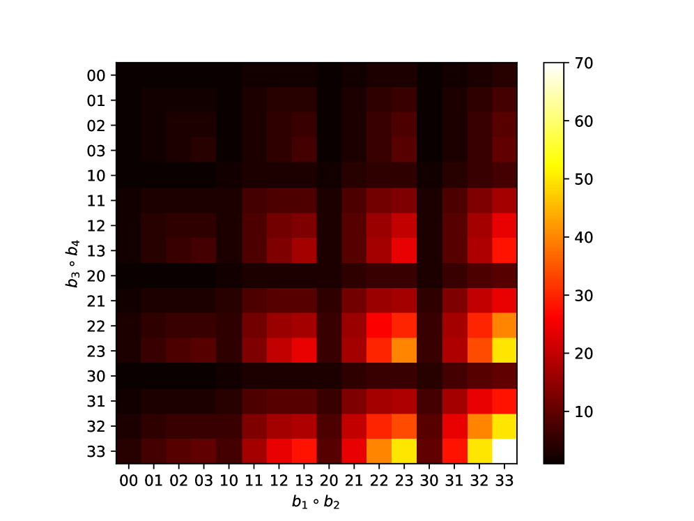
Figure 2: Number of configurations for each boundary condition for the square sampling $(b_{1},b_{2},b_{3},b4)$. The color coding reflects the multiplicity of configurations per boundary. For details see App. A

The quantum annealer produces a distribution of valid configurations that depend on the penalty factor $p$ of the QUBO matrix defined in Eq. (II), as well as hyper parameters that we discuss in detail in the next section. We classify the valid solution vectors per sub-lattice into histograms for each set of boundary conditions $b$, and sort them by monomer number $M$ and number of temporal dimers $D_{t}$, which encode the quark mass and temperature dependence. As the set of generated histograms $h_{p}(b,M,Dt)$ will depend on both the physical parameters and in particular the penalty factor $p$, the histogram is an estimate of the true distribution $h_{true}(b,M,Dt)$ that we obtain from exact enumeration (see Fig. 2 and App. A. We will discuss in Sec. III.3 and III.4 two methods to correct the histograms to obtain valid results.

$$\underbrace{\left(\begin{array}[]{c}\color[rgb]{1,0,0}{x_{1}^{(1)}}\\ \hline\cr\color[rgb]{0,0,1}{x_{2}^{(1)}}\\ \hline\cr\vdots\\ \hline\cr\color[rgb]{0,0,1}{x_{n-1}^{(1)}}\\ \hline\cr\color[rgb]{1,0,0}{x_{n}^{(1)}}\\ \end{array}\right)\,,\left(\begin{array}[]{c}\color[rgb]{0,0,1}{x_{1}^{(2)}}\\ \hline\cr\color[rgb]{0,0,1}{x_{2}^{(2)}}\\ \hline\cr\vdots\\ \hline\cr\color[rgb]{1,0,0}{x_{n-1}^{(2)}}\\ \hline\cr\color[rgb]{1,0,0}{x_{n}^{(2)}}\\ \end{array}\right)\,,\left(\begin{array}[]{c}\color[rgb]{0,0,1}{x_{1}^{(3)}}\\ \hline\cr\color[rgb]{0,0,1}{x_{2}^{(3)}}\\ \hline\cr\vdots\\ \hline\cr\color[rgb]{1,0,0}{x_{n-1}^{(3)}}\\ \hline\cr\color[rgb]{0,0,1}{x_{n}^{(3)}}\\ \end{array}\right)\,,\cdots\,,\left(\begin{array}[]{c}\color[rgb]{1,0,0}{x_{1}^{(N)}}\\ \hline\cr\color[rgb]{1,0,0}{x_{2}^{(N)}}\\ \hline\cr\vdots\\ \hline\cr\color[rgb]{0,0,1}{x_{n-1}^{(N)}}\\ \hline\cr\color[rgb]{0,0,1}{x_{n}^{(N)}}\\ \end{array}\right)}_{\text{$N$ solution vectors measured}}$$

Figure 3: Each column corresponds to a solution vector of a block QUBO matrix. The $x_{i}^{(j)}$ is a solution vector for each sub-lattice. We collect $x_{i}^{(j)}$ for fixed $i$ from $j=1,\cdots,N$ with $N$ solution vectors, and check the validity (blue: valid, red: invalid), see Eq. (19)

To be more specific, we measure the $N$ independent solution vectors $x^{(j)}$ ($j=1,\cdots,N$), blocked in $n$ separate sub-lattices $x^{(j)}_{i}$ ($i=1,\cdots,n$), as shown in Fig. 3. The boundary condition is the same for all $j$ at fixed $i$. Since not all configurations are valid in the sense that they fulfill the constraint Eq. (16) (red entries), it may happen that solutions vectors have invalid blocks. $N$ is typically large enough to ensure that for every $j$ there exists several valid sub-lattices $i$ from which we construct the histograms.

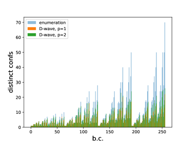
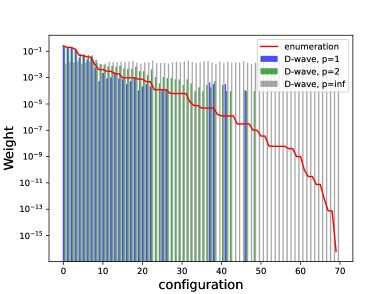
Figure 4: Comparison for $2\times 2$ sub-lattices between exact histograms from enumeration with those generated by D-wave for $p=1$ and $p=2$. Left: Comparison of the multiplicities for 256 different boundaries. Right: Comparison of the weights for a specific boundary (3,3,3,3) for $am_{q}=1.0$ and $\gamma=0.1$, with exact Boltzmann distribution compared to approximate distributions from D-Wave.

In Fig. 4, a comparison of the true histogram $h_{true}(b)$ by exact enumeration and the histogram $h_{p}^{b}$ obtained by the D-Wave quantum annealer for penalty factors $p=1,2,\infty$ is shown. Here, $b$ labels the 256 distinct boundary conditions $b=\{b_{1},\dots b_{4}\}$ in lexicographical order (left). The distribution for a specific boundary condition $b=(3,3,3,3)$ (right) is shown for quark mass $am_{q}=1.0$ and $\gamma=0.1$, now sorted by the Boltzmann weight $e^{-S}$. Both histograms are in good agreement for $p=1$, but this agreement deteriorates for larger $p$. This indicates that we have good overlap between the true and the approximate distributions of the $2\times 2$ sub-lattices, which is important to implement our strategy for large lattice volumes. How to correct the distribution for the small deviations is discussed in Sec. III.3 and III.4.

III.2 Optimizing hyper parameters

To maximize the efficiency of the simulation and obtain correct results, the hyper parameters chain_strength, num_reads, annealing_time should be optimized. Since the mapping from logical qubit to physical qubit is not trivial (we use automatized embedding which uses on average less than 2 physical qubits per logical qubit) it can happen that during the annealing process the embedding becomes invalid and results in broken ”chains”. For submitting a problem to the D-Wave system, one has to provide a value for the chain_strength, which can be chosen to reduce the number of broken chains. However, we cannot arbitrarily increase the value of chain_strength such that no broken chains occur, since too large a value adversely affects the number of obtained valid solutions. Thus some optimization is required.

We optimize the chain_strength to maximize the validity rate $v$, which is the number of valid solution vectors over all solution vectors:

$$v =\frac{1}{Nn}\sum_{j=1}^{N}\sum_{i=1}^{n}x_{i,\text{valid}}^{(j)}\,.$$ (19)

The QUBO matrix is rescaled by $Q_{max}$, which is the maximum absolute value of any element of the QUBO matrix before submitting to the D-wave solver. This results in rescaling the chain_strength to order one. For small values of chain_strength, the number of broken chains is large. As shown in Fig. 5, this results in a small validity rate. With increasing chain_strength, the validity rate grows with maximum around chain_strength is 1.0 to 1.2, depending on penalty factor $p$. Note that the weight matrix $W$ in the QUBO matrix has a block-diagonal structure, whereas the constraint matrix $A$ has long-range connectivity, requiring a larger chain_strength. However, if it is much larger than 1, the validity rate drops again [1].

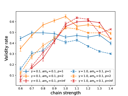
(a) annealing time=100, num_reads=800

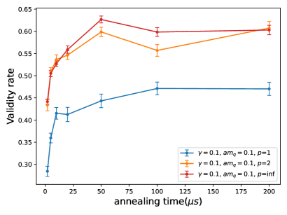
(b) annealing time dependence

Figure 5: The validity rate $v$ as a function of chain_strength on $2\times 2$ sub-lattice with ’3 3 3 3’ boundary condition. For penalty factor $p=1,2$ and infinite. $\gamma=0.1,1$, $am_{q}=0.1$. Right: $\gamma=0.1$, $am_{q}=0.1$

The number $N$ of solution vectors $x$ we request to be generated by the annealer is given by the parameter num_reads. As shown in Fig. 5, we optimize the annealing time per sample. The validity rate is saturated after the annealing time $100\mu s$. As increasing the annealing time, num_reads should be deceased accordingly. Hence we choose an annealing time of $100\mu s$. Since we have limited amount of quantum computing time, to balance the quantum computing time consumption and quality of the solution, we choose $\texttt{num\_reads}=200$. This allows us to generate histograms for more physical parameters.

III.3 Metropolis and Metropolis-Hastings

Although we know the exact distributions of the $2\times 2$ sub-lattices from enumeration, this is of no help with extending to finite periodic lattices: First, analytically extending to larger sub-lattices such as $4\times 4$ is not feasible due the exponential growth of computation involved. Second, a standard Metropolis algorithm attempting to glue the sub-lattices together would produce extremely small acceptance rates of about $0.1\%$ independent of the physical parameters. Alternative classical algorithms such as the Metropolis algorithm using the parallelization scheme as in Fig. 1 and sweeping through the 4 base points gives acceptance rates of about 20% for low temperatures $\gamma=0.1$, with a quark mass dependence as show in Fig. 6 (right).

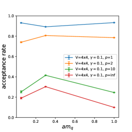
(a) Metropolis-Hastings (D-Wave)
p-dependence

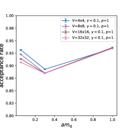
(b) Metropolis-Hastings (D-Wave)
volume-dependence

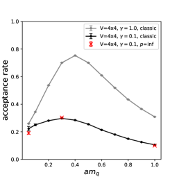
(c) Metropolis (classical)

Figure 6: Comparison of the acceptance rate. Left: for a $4\times 4$ lattice from Metropolis-Hastings, with $2\times 2$ sub-lattice histograms from D-Wave, for various penalty factors $p$. Center: illustrating independence of the acceptance rate of the volume. Right: Metropolis from classical computation, for $\gamma=0.1,1.0$. Metropolis-Hastings for $p=\infty$ reproduces the classical Metropolis acceptance rate.

In contrast, with the approximate distribution for $2\times 2$ sub-lattices measured by D-Wave for penalty factor $p=1$, we cannot incorporate the standard Metropolis algorithm, but have to use the Metropolis-Hastings algorithm:

$$P_{\rm accept} =e^{-S_{\rm new}+S_{\rm old}}\frac{h_{\rm old}}{h_{\rm new}}$$ (20)

with $e^{-S_{\rm new}}$ and $e^{-S_{\rm old}}$ the Boltzmann factors for the new/old configuration, and $h_{\rm new}$ and $h_{\rm old}$ the new/old histograms of the configuration. They are non-trivial: although they have the same boundary condition $b$, they differ in the specific distribution of monomers and dimers within the $2\times 2$ sub-lattice. The proposal probability $P_{\rm proposal}=\frac{h_{\rm old}}{h_{\rm new}}$ for a set of $2\times 2$ updates is not uniform as it is drawn from the measured histogram. As pointed out in Sec. III.1, these histograms have good overlap with the true distribution. Hence we expect that the Metropolis-Hastings algorithm will have a much larger acceptance rate, in particular also for low temperatures. The dependence of the acceptance probability on the penalty factors $p$ is shown in Fig. 6 (left). We can clearly see that $p=1$ has the largest acceptance rate, and that large $p$ will decrease the acceptance rate. In the limit $p\rightarrow\infty$, the weight matrix will not contribute to the QUBO matrix and the $2\times 2$ histograms become flat. Hence, due to $h_{old}=h_{new}$, the proposal probability drops out in the Metropolis-Hastings, which simplifies to standard Metropolis. The acceptance rate will hence be minimal as there is poor overlap with the important configurations given by the physical parameters. As shown in Fig. 6 (c), the $p=\infty$ acceptance rate agrees with the classical Metropolis algorithm. Recall that classical computations are in particular expensive for low temperatures (small $\gamma$), whereas the computational costs for the histograms measured by D-wave do not depend on $\gamma$. Also, the acceptance rate does not depend much on the volume as shown in Fig. 6 (b), as expected.

For the thermodynamic observables such as the chiral condensate and energy density, we show in Fig. 7 the $p$-dependence for $p=1,2,10,\infty$. We clearly see in the inset of Fig. 7 (a) that $p=1$ results in the smallest error, as it has the largest acceptance rate. For the large volume results in the next section, we hence always use $p=1$. We show in Fig. 8 for $p=1$ the volume-dependence of the chiral condensate and the energy density, for $V=4\times 4,8\times 8,16\times 16,32\times 32$ and compare the data with results from a classical computer using the worm algorithm.

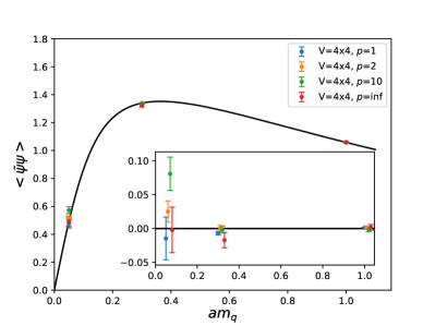
(a) Chiral Condensate at $\gamma=0.1$

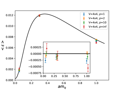
(b) Energy Density at $am_{q}=0.3$

Figure 7: Results from the Metropolis-Hastings algorithm, all for $\gamma=0.1$: chiral condensate (left) and energy density (right) for different $p$-values. The solid lines are analytic results from an exact enumeration. The inset figures show the difference between analytic and the numerical results. For any quark mass, $p=1$ has the smallest error.

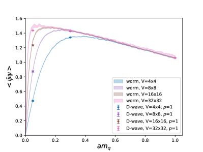
(a) Chiral Condensate at $\gamma=0.1$

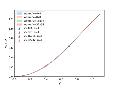
(b) Energy Density at $am_{q}=0.3$

Figure 8: Results of Metropolis-Hastings method for the chiral condensate for $p=1$ at $\gamma=0.1$ (left) and the energy density (right) for $p=1$ at $am_{q}=0.3$ for various 2-dimensional volumes.

III.4 Branching Strategy

Another promising method to correct the histograms that D-Wave provides to obtain valid results is to repeatedly branch into sub-branches, and statistically evaluate each branch to obtain expectation values for the chiral condensate and the energy. The essential idea of the branching strategy is to maximize quantum parallelization. While in the Metropolis-Hastings the same accept-reject step is required, the branching strategy performs accept-reject at each branch.

We start with a specific boundary condition (square sampling) with $b=(3,3,3,3)$, i.e. we choose $2\times 2$ sub-lattices with weights depending on the physical parameters $\gamma$ and $am_{q}$, as shown in Fig. 4 (right). The number of samples $N_{\rm branch}$ defines the branches. The same sample can be chosen multiple times in extreme cases (e.g. $am_{q}$ very large), although this is rare for physical parameters of interest (low temperatures, intermediate and small quark masses).

If we restrict to 2 dimensions, as we have 4 base points for $2\times 2$ sub-lattices, we have to repeat the above procedure 4 times and obtain further sub-branches, in total $N_{\rm branch}^{4}$ branches, each representing a valid configuration. While branching into $i$ sub-branches, the weight factor $w_{i}=e^{-S[i]}/h_{p,i}^{b}$ for each sample with index of depth $i$ multiplies the weight factors for all existing branches, where $h_{p}^{b}$ is the entry of the measured histogram, with $b$ the specific boundary condition. The final weight for each of the $N_{\rm branch}^{4}$ branches is

$$W_{\rm branch}=w_{1}\times w_{2}\times w_{3}\times w_{4}$$ (21)

Ultimately, to correct for bias, we must reweight our observable $\mathcal{O}$,

$$\langle OW_{\rm branch}\rangle/\langle W_{\rm branch}\rangle\ .$$

Unfortunately a limitation of this method so far is that the memory requirement for branching grows exponentially with $N_{\rm branch}$, preventing us from presenting results at this point in time.

IV Results

We have compared different 2-dimensional lattices in Sec. III.3 and extended to 4-dimensional volumes for the thermodynamic observables, as shown in Fig. 9, which includes a $4^{3}\times 4$ and $8^{3}\times 4$ lattice.

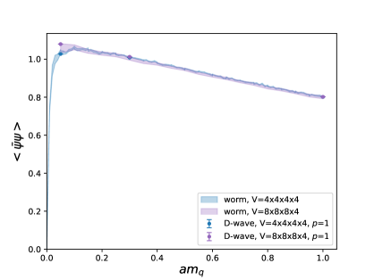
(a) Chiral Condensate at $\gamma=0.1$

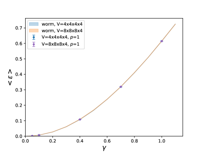
(b) Energy Density at $am_{q}=0.3$

Figure 9: 4-dim. results on $V=4\times 4\times 4\times 4$ and $8\times 8\times 8\times 4$. Left: chiral condensate at $\gamma=0.1$ for $am_{q}=0.05,0.3,1.0$. Right: energy density at $am_{q}=0.3$ for $\gamma=0.05,0.1,0.4,0.7,1.0$.

We are particularly interested in the chiral limit $am_{q}\rightarrow 0$ for the chiral condensate, and the low temperature limit $\gamma\rightarrow 0$ for the energy density, as these limits are particularly interesting from the physics point of view, and expensive with classical computers. We also present “extrapolated results”, for which we use a histogram at fixed quark mass and temperature $\gamma$ and run the Metropolis-Hastings for smaller quark masses and/or temperatures, given that there is still sufficient overlap with the corresponding target distributions. We demonstrated that these extrapolations are under control for all 2-dimensional volumes under investigation: the lattices $4\times 4$, $8\times 8$, $16\times 16$, $32\times 32$, as shown in Fig. 10. As this works remarkably well, we can reduce drastically the number of histograms that have to be generated on the annealer for the set of physical parameters.

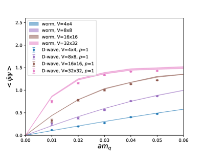
(a) Chiral extrapolation at $\gamma=0.1$

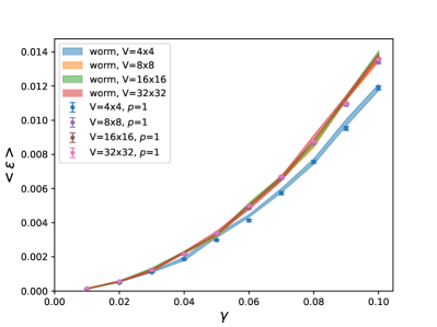
(b) Low temperature extrapolation at $am_{q}=0.3$

Figure 10: Chiral extrapolation (left) from histograms at $am_{q}=0.05$, $\gamma=0.1$, $p=1$, obtained via Metropolis-Hastings for several quark masses $am_{q}\leq 0.05$ and various volumes. Right: low temperature extrapolation from $am_{q}=0.3$, $\gamma=0.1$, $p=1$ for several $\gamma\leq 0.1$. The bands are obtained by worm simulation on the classical computer.

V Conclusion

We developed an algorithm to simulate ${\rm U}(3)$ gauge theory in the strong coupling limit for large 2-dimensional and 4-dimensional volumes on a quantum annealer. In particular, we made use of an hybrid quantum/classical approach, whereby we determined the histograms in the dual variables relevant to the QUBO formalism via the D-Wave quantum annealer, and than ran the Metropolis-Hastings algorithm based on these histograms on a classical computer. We optimized the hyper parameters to reduce the compute time on the annealer, and found optimal values for annealing_time and chain_strength. Also, the penalty factor $p$ that balances the weight matrix and the constraint in the QUBO matrix, for which the quality of the histograms is best was determined to be $p=1$, resulting in large acceptance rates.

Further improvements can be obtained by using the quantum parallelization more extensively and efficiently while branching our sub-lattices. This would require a better understanding of how the number of branches can be optimized with respect to compute time and memory requirement, in particular in four dimension. We are actively investigating this option.

Extending to ${\rm SU}(3)$ and including gauge corrections are another important next step towards a more realistic effective theory of lattice QCD. The first aspect includes baryons while the second aspect includes gluon propagation. The dual representation is well established for both extensions, and again can be mapped on binary vectors. However, these formulations will require more logical qubits. Still, it remains feasible to map the logical qubits required for the QUBO matrix to the physical qubits on the annealer. However, while the histograms required for this work, given square sampling, had $4^{4}$ different boundaries to classify the histograms, these generalizations will require up to $16^{4}$ different boundaries, for which the histograms can no longer be pre-computed on D-wave. Instead they need to be computed during Metroplis-Hastings in between the updates, whenever required. Studying more realistic effective theories will introduce two more physical parameters [14]: the quark chemical potential $\mu_{q}$, and the inverse gauge coupling $\beta$ that is related to the lattice spacing $a$. We will report on our findings using the same approach via histograms determined on the annealer in a subsequent publication.

Appendix A Exact Enumeration

From exact enumeration, we obtain for $2\times 2$ sub-lattices with fixed boundary conditions (the building blocks of square sampling) in total 2350 distinct configurations, that are distributed over 256 distinct boundaries $(b_{1},b_{2},b_{3},b_{4})$, with $b_{i}\in\{0,1,2,3\}$.

If we further distinguish the sub-lattice configurations by its monomer number $M$ and number of temporal dimers $D_{t}$, we obtain refined multiplicities. In the Tab. 2 we give the multiplicities in these sectors $M$, $D_{t}$.

$M$				$D_{t}$				sum
	0	1	2	3	4	5	6
0	16	18	17	10	6	2	1	70
1	48	60	48	28	12	4	0	200
2	92	110	82	40	14	2	0	340
3	132	148	96	40	8	0	0	424
4	153	154	88	26	3	0	0	424
5	148	132	60	12	0	0	0	352
6	124	92	32	4	0	0	0	252
7	88	52	12	0	0	0	0	152
8	54	24	3	0	0	0	0	81
9	28	8	0	0	0	0	0	36
10	12	2	0	0	0	0	0	14
11	4	0	0	0	0	0	0	4
12	1	0	0	0	0	0	0	1
sum	900	800	438	160	43	8	1	2350

Table 2: Multiplicities from exact enumeration on $2\times 2$ sub-lattices with fixed boundary conditions sorted by monomer number $M$ and temporal dimer $D_{t}$

$M$								$B$						sum
	0	1	2	3	4	5	6	7	8	9	10	11	12
0	1	0	4	0	10	0	20	0	19	0	12	0	4	70
1	0	4	0	16	0	40	0	64	0	52	0	24	0	200
2	0	0	10	0	40	0	88	0	116	0	74	0	12	340
3	0	0	0	20	0	72	0	136	0	144	0	52	0	424
4	0	0	0	0	31	0	100	0	158	0	116	0	19	424
5	0	0	0	0	0	40	0	112	0	136	0	64	0	352
6	0	0	0	0	0	0	44	0	100	0	88	0	20	252
7	0	0	0	0	0	0	0	40	0	72	0	40	0	152
8	0	0	0	0	0	0	0	0	31	0	40	0	10	81
9	0	0	0	0	0	0	0	0	0	20	0	16	0	36
10	0	0	0	0	0	0	0	0	0	0	10	0	4	14
11	0	0	0	0	0	0	0	0	0	0	0	4	0	4
12	0	0	0	0	0	0	0	0	0	0	0	0	1	1
sum	1	4	14	36	81	152	252	352	424	424	340	200	70	2350

Table 3: Multiplicities from exact enumeration on $2\times 2$ sub-lattices with fixed boundary conditions sorted by monomer number $M$ and sum of boundary conditions $B=b_{0}+b_{1}+b_{2}+b_{3}$

References

- Kim et al. [2023a] J. Kim, T. Luu, and W. Unger, U(N) gauge theory in the strong coupling limit on a quantum annealer, Phys. Rev. D 108, 074501 (2023a), arXiv:2305.18179 [hep-lat] .
- Kim et al. [2023b] J. Kim, T. Luu, and W. Unger, Testing importance sampling on a quantum annealer for strong coupling SU(3) gauge theory, in 40th International Symposium on Lattice Field Theory (2023) arXiv:2311.07209 [hep-lat] .
- Lund et al. [2017] A. P. Lund, M. J. Bremner, and T. C. Ralph, Quantum sampling problems, BosonSampling and quantum supremacy, npj Quantum Inf. 3, 15 (2017).
- Ghamari et al. [2024] D. Ghamari, R. Covino, and P. Faccioli, Sampling a Rare Protein Transition Using Quantum Annealing, J. Chem. Theor. Comput. 20, 3322 (2024).
- Vuffray et al. [2022] M. Vuffray, C. Coffrin, Y. A. Kharkov, and A. Y. Lokhov, Programmable Quantum Annealers as Noisy Gibbs Samplers, PRX Quantum 3, 020317 (2022), arXiv:2012.08827 [quant-ph] .
- Wild et al. [2021] D. S. Wild, D. Sels, H. Pichler, C. Zanoci, and M. D. Lukin, Quantum sampling algorithms, phase transitions, and computational complexity, Phys. Rev. A 104, 032602 (2021), arXiv:2109.03007 [quant-ph] .
- Jattana [2024] M. S. Jattana, Quantum annealer accelerates the variational quantum eigensolver in a triple-hybrid algorithm, Phys. Scripta 99, 095117 (2024), arXiv:2407.11818 [quant-ph] .
- Izquierdo et al. [2021] Z. G. Izquierdo, T. Albash, and I. Hen, Testing a Quantum Annealer as a Quantum Thermal Sampler, ACM Trans. Quant. Comput. 2, 7 (2021), arXiv:2003.00361 [quant-ph] .
- Sandt and Spatschek [2023] R. Sandt and R. Spatschek, Efficient low temperature Monte Carlo sampling using quantum annealing, Sci. Rep. 13, 6754 (2023).
- Ghamari et al. [2022] D. Ghamari, P. Hauke, R. Covino, and P. Faccioli, Sampling rare conformational transitions with a quantum computer, Sci. Rep. 12, 16336 (2022), arXiv:2201.11781 [quant-ph] .
- Shibukawa et al. [2024] R. Shibukawa, R. Tamura, and K. Tsuda, Boltzmann sampling with quantum annealers via fast Stein correction, Phys. Rev. Res. 6, 043050 (2024), arXiv:2309.04120 [cond-mat.stat-mech] .
- Systems [2019] D.-W. Systems, Pegasus: The Topology of D-Wave Quantum Processors, Tech. Rep. (D-Wave Systems Inc., 2019) https://docs.dwavesys.com/docs/latest/c_gs_4.html#topology-intro-pegasus.
- Rossi and Wolff [1984] P. Rossi and U. Wolff, Lattice QCD With Fermions at Strong Coupling: A Dimer System, Nucl. Phys. B248, 105 (1984).
- Kim et al. [2023c] J. Kim, P. Pattanaik, and W. Unger, Nuclear liquid-gas transition in the strong coupling regime of lattice QCD, Phys. Rev. D 107, 094514 (2023c), arXiv:2303.01467 [hep-lat] .