Dynamic constructions of hyperbolisms
of plane curves:
an automated exploration of geometric loci
Abstract
Hyperbolism of a given curve with respect to a point and a line is an interesting construct, a special kind of geometric locus, not frequent in the literature. While networking between two different kinds of mathematical software, we explore various cases, involving quartics, among them the so-called Külp quartic and topologically equivalent curves, and also an example with a sextic and a curve of degree 12. By a similar but different way, we derive a new construction of a lemniscate of Gerono. First, parametric equations are derived for the curve, then we perform implicitization Gröbner bases packages and using elimination. The polynomial equation which is obtained enables to check irreducibility of the constructed curve.
Thierry Dana-Picard
Jerusalem College of Technology and Jerusalem Michlala College
Jerusalem, Israel
ndp@jct.ac.il
1 Introduction
1.1 The needed dialog between two kinds of mathematical software
Prior to the development of Computer Algebra Systems (CAS) and Dynamic Geometry Software (DGS), mechanical devices were used to draw specific curves [28]; spirographs were among the most popular and enabled to draw epitrochoids and hypotrochoids111See https://mathcurve.com/courbes2d.gb/epitrochoid/epitrochoid.shtml and https://mathcurve.com/courbes2d.gb/hypotrochoid/hypotrochoid.shtml. and other related curves. Here, instead of mechanical devices, we use software, both a DGS (GeoGebra) and a CAS (Maple). The first one enables to construct and explore the curves, their shape and topology, sometimes providing polynomial equations but not always. We use then the CAS in order to perform algebraic computations and derive polynomial equations for the curves under study. Afterwards it is possible to copy-paste the formulas to the DGS and to analyze the curves with its dynamical features. This CAS-DGS collaboration provides a useful environment for the exploration of new constructs, as in [14]. Such a dialog between the two kinds of software has been used for example in [11, 9],and for years has been wished to be more automatic [24].
In this work, the curve are determined first by parametric equations. Implicitization is important, as a polynomial presentation may provide information whether the curve is irreducible or not (see [21], chap. 1). The algebraic part of the work is based on the theory of Gröbner bases and on Elimination; see [7, 27]. We may refer also to [2], in particular for the non familiar reader who can see how to work out elementary examples by running the algorithms ”by hand”. Note that Maple has an implicitize routine in its package algcurves, based on [6]. Irreducibility is also checked with automated methods; see Section 2.
Mathematical objects cannot be grasped with hands, and are approached using numerous registers of representations [17]; the classical registers for plane curves are graphical, numerical and algebraic. Parametric representations and implicit representations as two subregisters of the algebraic one. The study is made rich and efficient by switching between registers, but switching from parametric to implicit and from implicit to parametric are non trivial tasks; see [22, 26, 27, 7]. In some cases, the switch is impossible.
Switching between different representations of plane curves is an important issue, with numerous applications in computer aided design and other fields. In [29], Wang emphasizes the role in computer aided geometric design and modeling. He develops ”an extremely simple method that converts the rational parametric equations for any curve or surface into an implicit equation” (we recommend also the vast bibliography there in the paper) . He uses Gröbner bases, resultants, etc. In our work here, we transform the obtained parametric equations into parametric rational presentations, then into polynomial equations. We use Maple’s PolynomialIdeals package and elimination to derive implicit equations. It is often easier to analyze the topology of a curve using an implicit presentation than a parametric presentation. Anyway, both enable the study and classification of singular points.
1.2 Plane curves defined as geometric loci
Plane algebraic curves are a classical topic, to which numerous books have been devoted, such as [31]. Websites are devoted to curves (and surfaces) such as Mathcurve (http://mathcurve.com). Full catalogues of curves of degree 2,3 and 4 exist, and partial catalogues for degree 6. Some of them are constructed as geometric loci. The bifocal definition of ellipses and hyperbolas is generally the first example met by students. Cassini ovals (also called spiric curves) and Cayley ovals are more advanced examples. Recently, some octic curves (curves defined by polynomials of degree 8) have been described as geometric loci in relation with a classical theorem of plane geometry, namely Thales second theorem [12, 15]. The present paper shows a bunch of curves, more or less classical, appearing as geometric loci by construction of hyperbolisms.
Our concern is the construction and study of plane curves as hyperbolism of classical curves, according to the definition in the Mathcurve website [20]:
Definition 1.1.
The hyperbolism of a curve with respect to a point and a line is the curve , locus of the point defined as follows: given a point on , the line cuts at ; is the projection of on the line parallel to passing by .
Remark 1.2.
Analytically, if the line is given by the equation , the transformation of into can be written ; it is quadratic, so an algebraic curve of degree is transformed into an algebraic curve of degree at most . The 2nd coordinate makes the connection with hyperbolas, whence their name hyperbolism.
By definition, hyperbolisms of curves are a subtopic of geometric loci, which are a classical topic, from middle school to university. The last decades have seen numerous works devoted to automated methods in Geometry, such as [1, 3, 4] and [23], where loci are one of the main topics for which automated methods have been developed, and implemented in GeoGebra-Discovery222A freely downloadable companion to GeoGebra, available fromhttps://github.com/kovzol/geogebra-discovery. A large number of versions of automated commands exist, we use here only a few of them, mostly GeoGebra’s Locus(Point Creating Locus,Point) and Locus(Point Creating Locus,Point). The place holders are called respectively the Tracer and the Mover in the above mentioned papers. The automated command provides a plot of the curve, sometimes also an implicit equation. For this it uses numerical methods. In the companion package GeoGebra-Discovery, this has been supplemented by symbolic algorithms yielding more precise answers. For the algebraic work, we switched to the Maple software, especially for implicitization, but not only.
The notion of a hyperbolism has been presented to a small group of in-service mathematics teachers, learning towards an advanced degree M.Ed. These teachers had previous knowledge including the perpendicular bisector of a segment, a circle, conics, etc. as geometric loci, but almost neither CAS nor DGS literacy. The outcome of their work was double: the development of new perspectives in geometry and acquisition of technological skills. They had neither true and the general atmosphere of the course was to show new mathematical topics in a technology-rich environment and develop technological skills. The feedback was very positive, and true curiosity at work.
2 First easy examples
2.1 Hyperbolism of a circle centered at the point and the line is tangent to the circle
We consider the circle centered at the origin with radius . The line has equation and is thus tangent to the circle . A point is given by where . The line has thus equation and intersects the line at . It follows that the point has coordinates
| (1) |
Equation (1) is a parametric presentation of the geometric locus that we are looking for. Figure 1 shows a screenshot of a GeoGebra session for this question. The requested curve has been obtained using the LocusEquation() command. It could have been obtained also with the LocusEquation(Point Creating Locus Line , Slider ), after entering directly the parametrization (1), but in this case the new construct is independent of what has been done previously.
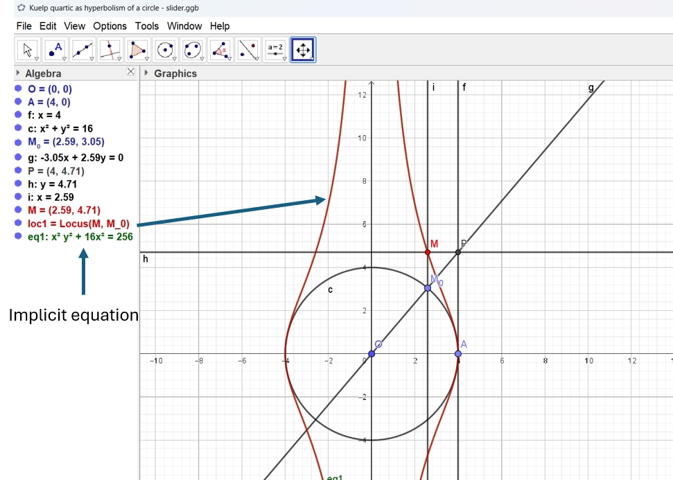
The plots corresponding to the 2 last rows in the algebraic window overlap each other, therefore only one plot is viewed. Nevertheless, they are considered by the software as 2 different objects.
In this session, the radius may be changed, but the equation of the geometric locus remains of the same form. In Figure 1, and the geometric locus has equation
| (2) |
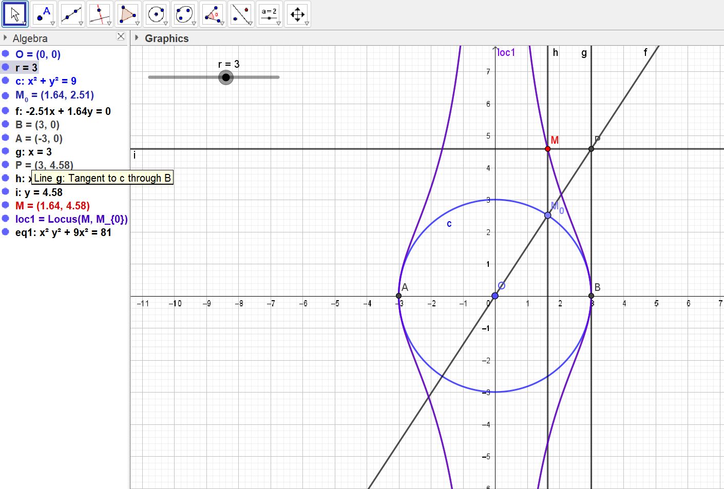
which is identified as the equation of a so-called Külp quartic333A curve studied in 1878 by Külp; see https://mathcurve.com/courbes2d/kulp/kulp.shtml. A GeoGebra session444https://www.geogebra.org/m/md4f8aaa may help to visualize the construct for various values of the radius. Slightly different ways to construct the hyperbolism may be chosen, and for some of them an implicit equation is not available. The user has to modify his protocol to have it ”more geometric” (v.i. Section 4). Sometimes, GeoGebra-Discovery displays a message telling that the construction involves steps which are not supported by the command LocusEquation. In our applet, the tangent has not been constructed directly with its equation, as in Figure 1, but using the Tangent command of the software, which is important as part of a geometric construct; see Figure 2.
In order to derive from Equation (1) a polynomial equation, we use the following substitution, as in [11]:
| (3) |
We apply the following Maple code:
xk := r*cos(t); yk := r*sin(t)/cos(t);
xkrat := subs(cos(t) = (-u^2 + 1)/(u^2 + 1), xk);
ykrat := subs(cos(t) = (-u^2 + 1)/(u^2 + 1),
         subs(sin(t) = 2*u/(u^2 + 1), yk));
p1 := x*denom(xkrat) - numer(xkrat);
p2 := y*denom(ykrat) - numer(ykrat);
J := <p1, p2>;
JE := EliminationIdeal(J, {r, x, y});
The output is an ideal with a unique generator, providing the following equation (for any real ):
| (4) |
Note the dependence of the coefficients in Equation (4) on the radius of the circle. Using Maple’s command evala(AFactor(…), we check that the left hand side in Equation (4) is an irreducible polynomial. This means that the 2 components of the curve described by this equation cannot be distinguished by algebraic means, i.e. they are not 2 distinct components of the curve (see [21], p.17-18).
2.2 Hyperbolism of an ellipse
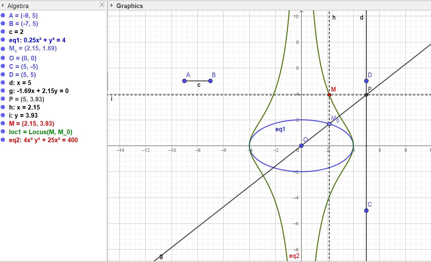
We generalize slightly the situation of subsection 2.1 and consider now an ellipse whose equation is , where and are positive parameters555GeoGebra applets are available at https://www.geogebra.org/m/eqywkwcw and https://www.geogebra.org/m/tfnrwaqh. Here too, the point is the origin. The line has equation , i.e. is tangent to the ellipse and parallel to the axis. A point is given by where . The line has thus equation and intersects the line at . It follows that the point has coordinates
| (5) |
Remark 2.1.
The segment in the upper left corner of Figure 3 comes instead of a slider for a parameter which is involved in the implicit equation of the ellipse. This, in order to have the ellipse dependent on a geometric construct. Actually, the ellipse itself could have been constructed as a geometric loci, but in such a case GeoGebra’s command LocusEquation may provide a plot and an implicit equation, but not the possibility to use the command Point on Object.
We apply a Maple code similar to the code in the previous subsection666Maple’s implicitize command did not always provide an answer.. The output provides an equation for the hyperbolism of the ellipse:
| (6) |
Using the same tool as in previous section, we show that obtained curve is irreducible. Note that it is not a Külp quartic (the coefficient of is not the square of the free coefficient). The equations are quite similar, but not identical. Figure 4 shows how a GeoGebra applet may help to understand that, for various values of the axes of the ellipse, the obtained curves have the same topology. The exploration leads to proving that two curves in this family are obtained from each other by an affinity whose axis is the axis and the direction is perpendicular to it. Moreover, this may be an opportunity to explore in class the similarities and the differences of these quartics, Külp quartic, and also the Witch of Agnesi (which is a cubic).
Remark 2.2.
Denote . We have: and . It is easy to show that the system of equations has no solution (actually solves the system, but the origin does not belongs to the curve). Therefore the curve has no singular point.
Remark 2.3.
Assuming that at inflexion points the curvature is equal to 0, it is possible to look for candidates using the following code:
with(Student[VectorCalculus]);
Curvature(<a*cos(t), b*tan(t), t>, t);
simplify(%);
infl := solve(% = 0, t);
allvalues(infl[1]);
Different issues may appear. First the meanings of in the two packages PolynomialIdeals and VectorCalculus are different, therefore we suggest to introduce the 2nd one only after the first one has been used. Second, the answer for general parameters and may be heavy; it may be wiser to use them with specific values. Finally, this provides values of the parameter which can correspond to points of inflexion, but not only. More verifications are needed.
Remark 2.4.
The given ellipse is the image of the circle whose equation is by the affine transformation . It is easily proven that the quartic obtained here is the image by the same transformation of the Külp quartic found in the previous subsection.
3 Hyperbolism of a circle with respect to a line secant to the circle
3.1 The circle is centered at the origin
Other quartics can be obtained as hyperbolisms of circles.
We consider a circle centered at the origin with radius and the line with equation , where . Figure 5 is a screenshot of a GeoGebra applet777https://www.geogebra.org/m/pwrx2uzf; a related applet is available at https://www.geogebra.org/m/x22etuhc.); the line is a secant to the circle .
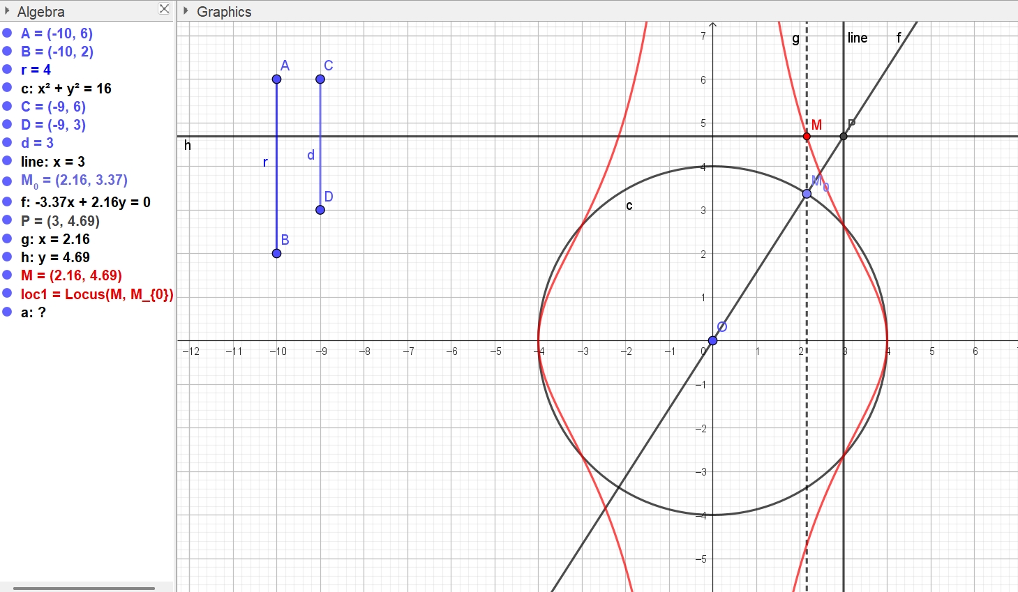
We perform the same construction as in subsection 2.1, and obtain a plot of the geometric locus, but cannot obtain an implicit equation with the command LocusEquation. Therefore, we need to make the algebraic computation using the CAS. Note that, even when changing the value of by changing the length of the corresponding segment AB, the implicit equation is not obtained.
f := -r^2 + x^2 + y^2;
li := y = r*sin(t) + sin(t)*(x - r*cos(t))/cos(t);
yP := subs(x = d, rhs(li));
xM := r*cos(t);
yM := yP;
p1 := x - xM;
p2 := y - yM;
p1 := subs(cos(t) = (-u^2 + 1)/(u^2 + 1), p1);
p2 := subs(cos(t) = (-u^2 + 1)/(u^2 + 1), subs(sin(t) = 2*u/(u^2 + 1), p2));
p1 := simplify(p1*denom(p1));
p2 := simplify(p2*denom(p2));
J := <p1, p2>;
JE := EliminationIdeal(J, {d, r, x, y});
The output provides an implicit equation for the hyperbolism. After simplification, it reads as follows:
| (7) |
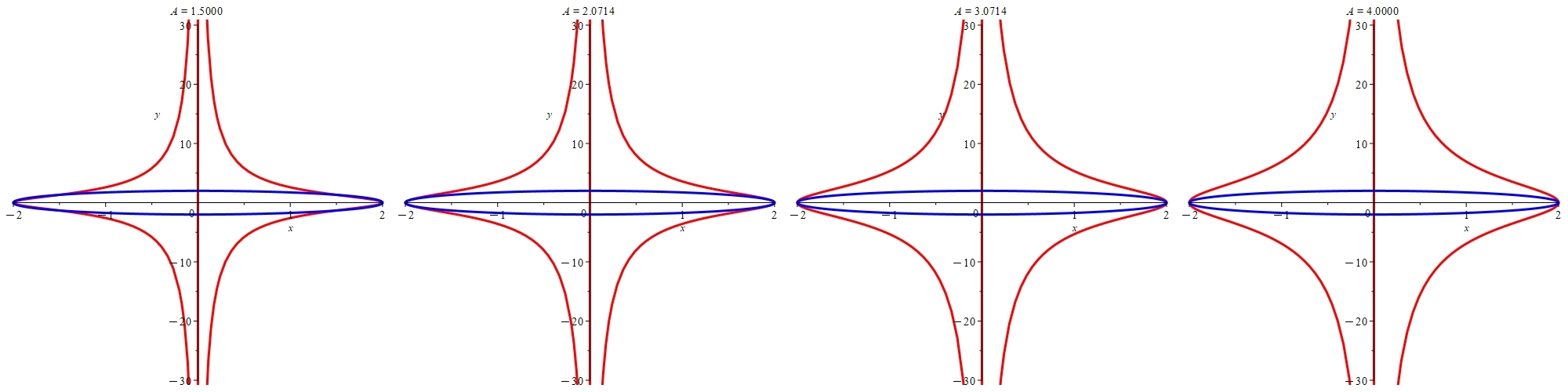
As expected, for , we have Equation (4). Figure 6 shows hyperbolisms of the same circle for 4 different lines whose respective equations are , , and , from the innermost to the outermost curve.
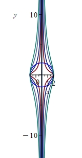
Their differences are emphasized in Figure 7, in an orthogonal but not orthonormal system of coordinates (therefore, the circle does not ”look like” a circle) . These are screenshots of an animation programmed with Maple, with the animate command, as follows:
ac := animate(plot, [[r*cos(t), subs(d = A, yP), t = 0 .. 2*Pi]],
       A = 0.5 .. 4, frames = 50, color = red, thickness = 3)
Here too, as in subsection 2.2, the animation provides a visualization of the fact that for different values of the parameters, the obtained curve has the same topology.
3.2 The circle passes through the origin
We consider now a circle passing through the origin and centered on the axis. The circle has equation . We take a line , where and the point is the origin. The construction is displayed in Figure 8. The segments on the left are used instead of sliders.
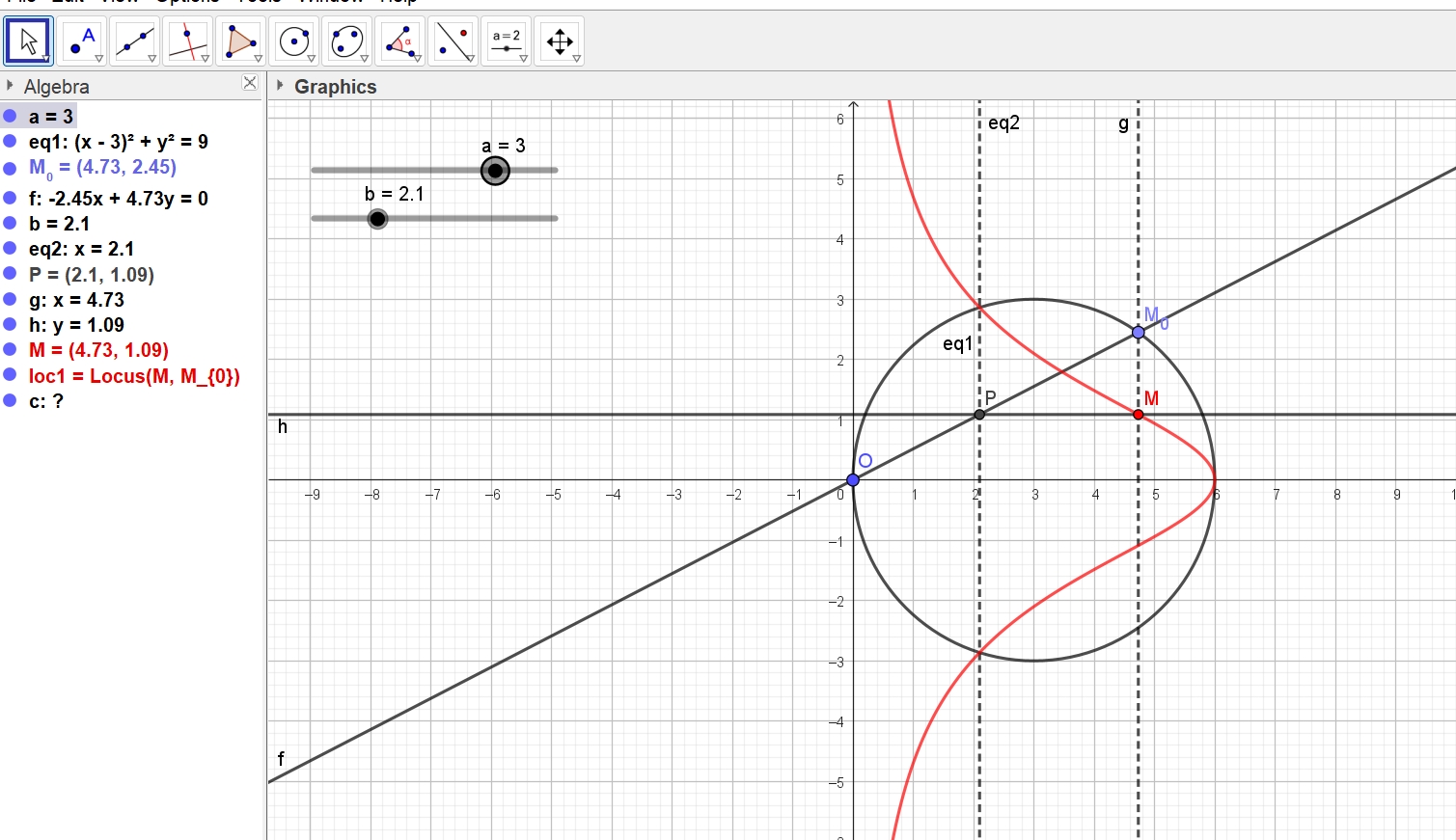
A plot of the geometric locus of the point (the Tracer) when (the Mover) runs over the circle is obtained by the Locus command. Not as in the previous section, the command LocusEquation does not provide an answer. Therefore, algebraic computations have to be performed using the CAS.
First, we derive a parametric presentation for the circle , using the intersection of the circle and of a line through the origin with slope (pay attention that this will be thw generic line )
| (8) |
For the point : if , then and has coordinates
| (9) |
We define polynomials
| (10) |
Let . By elimination of the parameter , we obtain the following implicit equation of degree 3:
| (11) |
Note that for , i.e. the line is tangent to the circle at the end point of a diameter passing by the origin, the curve is a Witch of Agnesi.
4 Piriform quartics
4.1 Hyperbolism of a piriform quartic curve
We refer to [19] for the implicit and parametric presentation of the curve. A piriform curve is a quartic whose equation is
| (12) |
where and are positive parameters. In Figure 9 (a screenshot of a GeoGebra applet888https://www.geogebra.org/m/smcehrzy), these parameters are determined by 2 segments, in order to have a purely geometric construction.
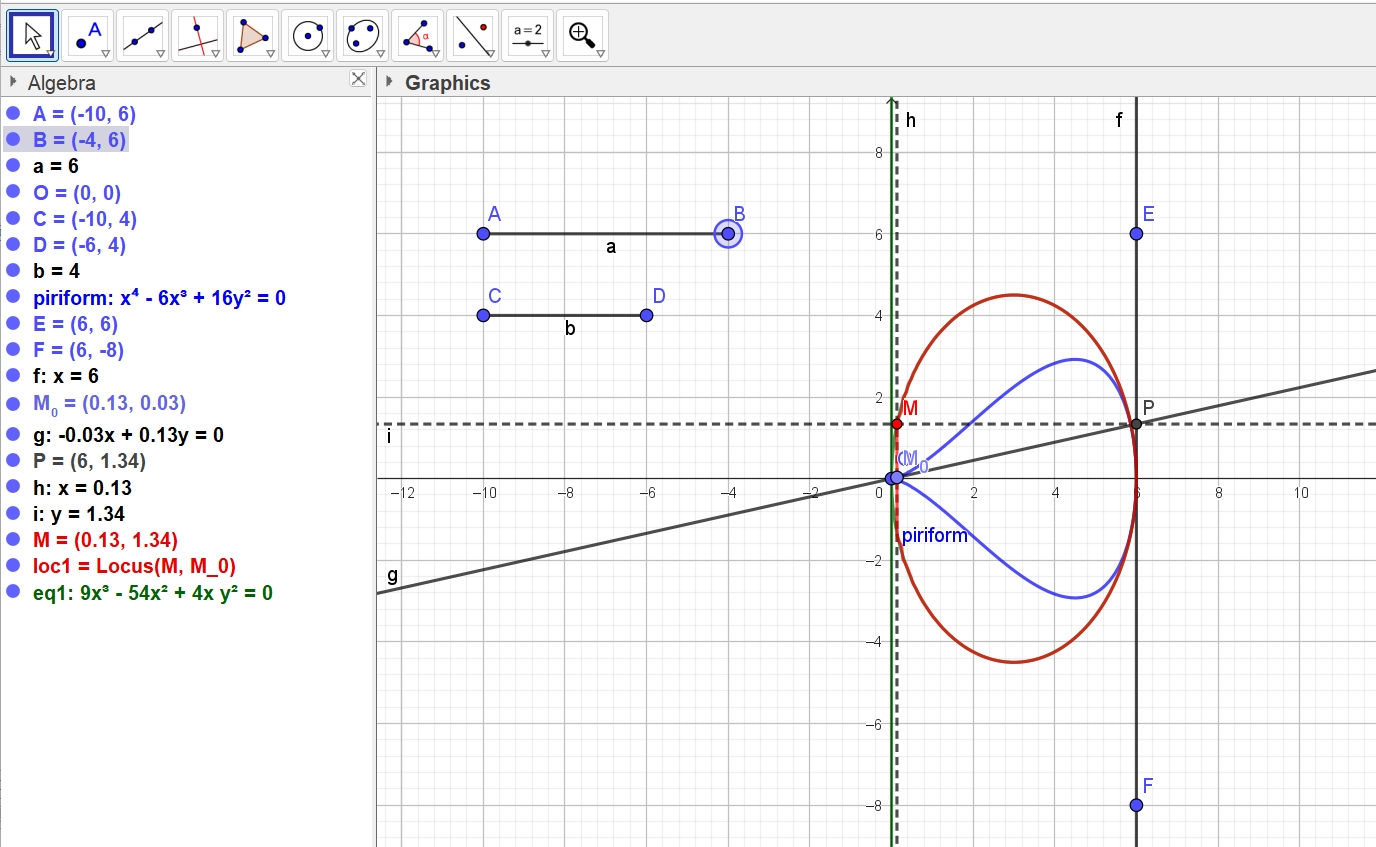
This figure correspond to the case . A plot is obtained and, simultaneously, an implicit equation, which reads as follows:
| (13) |
The factor determines the axis, emphasized in the Figure. This component is irrelevant to the geometric question; it appears because issues related to Zariski topology. Such issues are discussed in [10], and are beyond the scope of the present article. The 2nd factor determines an ellipse, whose equation can be written as follows:
| (14) |
enabling to find the geometric characteristic elements of the ellipse. This is the desired hyperbolism of the piriform curve.
In order to perform the algebraic computations, it is worth to begin with a parametric presentation of the curve . We may use a trigonometric parametrization999It is given at https://mathcurve.com/courbes2d.gb/piriforme/piriforme.shtml.:
| (15) |
but we have to transform it into a rational parametrization. We choose a different way. Any line but the axis through the origin intersects again the curve . Let be the line whose equation is . We use the following Maple code:
pear := b^2*y^2 - x^3*(a - x);
l := -t*x + y;
solve({l = 0, pear = 0}, {x, y});
par := allvalues(%[2]);
The output gives two components, given by:
| (16) |
and
| (17) |
We work now with the first component, the 2nd one can be treated exactly in the same way.
Denote . By construction, we have:
| (18) |
Now we use the following Maple code:
p1 := x - a/2 =sqrt(-4*b^2*t^2 + a^2)/2;
p1 := p1^2;
p1 := lhs(p1) - rhs(p1);
p2 := -a*t + y;
J:=<p1,p2>;
JE := EliminationIdeal(J, {a, b, x, y})
G := Generators(JE)[1];
whose output is the polynomial
| (19) |
We have
| (20) |
Rewriting the equation under the form
| (21) |
which is equivalent to
| (22) |
we identify that the requested curve is an ellipse.
Remark 4.1.
The obtained hyperbolism has been identified as an ellipse by algebraic means. This appears also in the GeoGebra applet, but a slight modification may induce a big change, and the implicit equation may not be obtained. An experimental way to check that the curve is an ellipse consists in marking 5 arbitrary points on the curve (with the Point on Object command) and determine a conic by 5 points on it (there is a button driven command for this). This is a numerical checking, not a symbolic proof, but may enable students to proceed further. Of course, the algebraic computations that we performed with the CAS are a must.
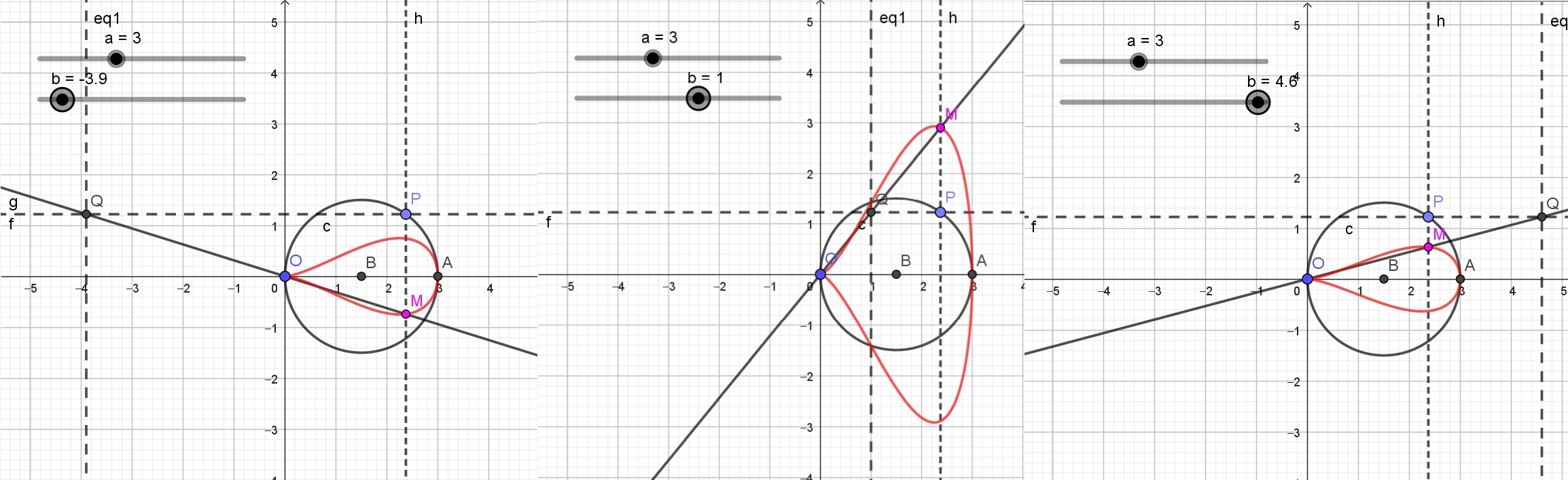
4.2 A piriform curve as antihyperbolism of a circle
The choice of the original curve in previous subsection incites to have a look at piriform curves from another point of view; see [20, 19].
Definition 4.2.
With the notations of Definition 1.1, the inverse transformation is called antihyperbolism.
Screenshots of a GeoGebra applet101010https://www.geogebra.org/m/yfq7wmqz are displayed in Figure 10. Exploration using the sliders show that for , the piriform curve lies inside the circle and is tangent to it at . For , the curve is part inside and part outside of the circle, and is still tangent to the circle at , but from outside.
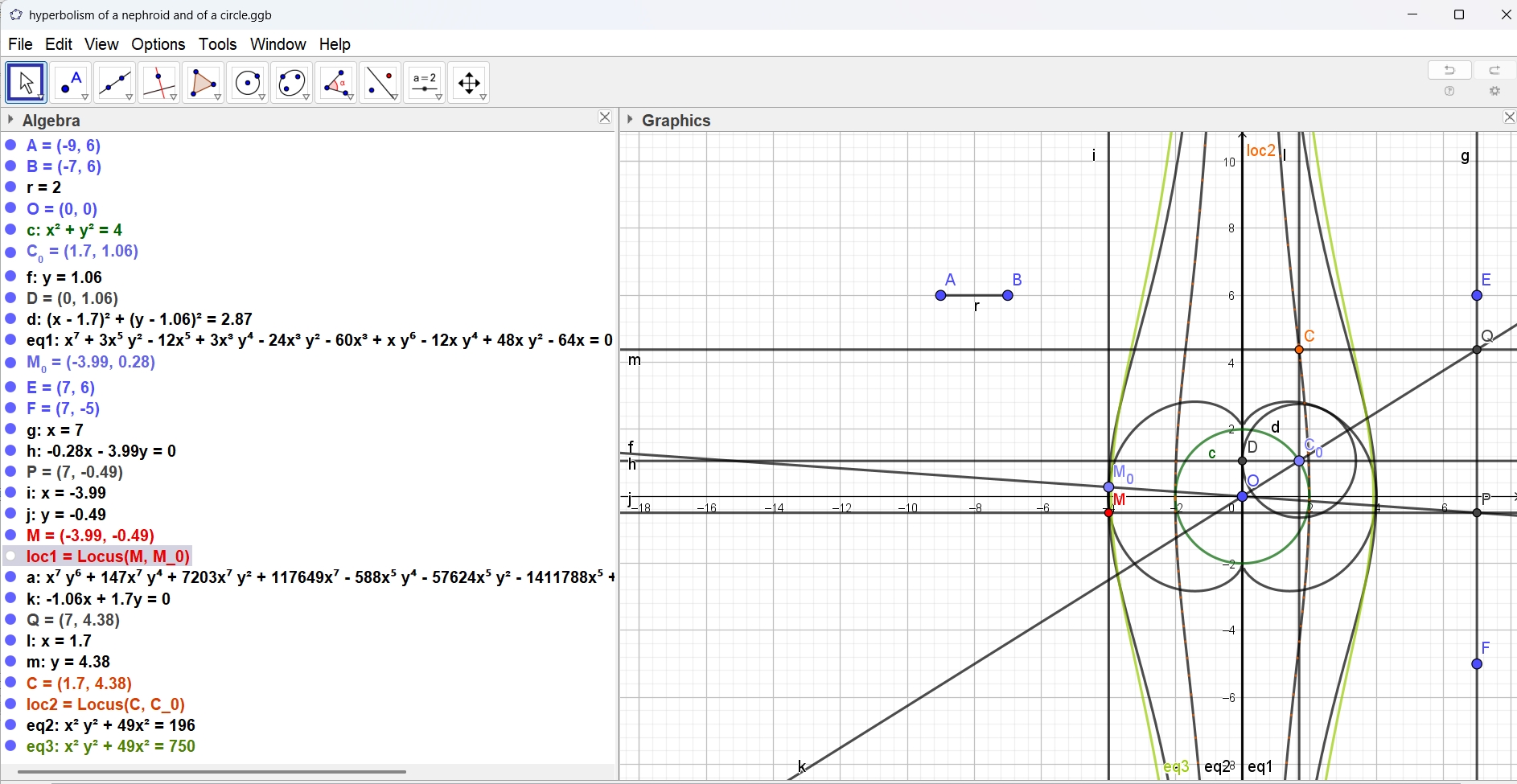
5 Hyperbolism of a nephroid
Let be a circle whose center is at the origin. The envelope of the family of circles centered on and tangent to the axis is a sextic called a nephroid [16]. By that way the curve has been constructed in Figure 11, which is a screenshot of a GeoGebra applet111111https://www.geogebra.org/m/pyhk9qvr. We denote the nephroid by . Later, this figure will enable to compare the hyperbolism of with a hyperbolism of a circle, as described in Subsection 2.1.
A general implicit equation for a nephroid is
| (23) |
where is a positive parameter. The curve can also be described by a parametric presentation
| (24) |
To construct a hyperbolism of with respect to the origin and to a vertical line, we follow the same path as in previous sections. This begins with deriving from Equation (24) a rational parametrization. Applying the substitution in Equation (3), we obtain:
| (25) |
The coordinates of are thus
and the coordinates of are
| (26) |
We run now the following Maple code, similar to what we did already:
p1 := x*denom(xM) - numer(xM);
p2 := y*denom(yM) - numer(yM);
J := <p1, p2>;
JE := EliminationIdeal(J, {a, b, x, y});
G := Generators(JE)[1];
evala(AFactor(G));
The last command is intended to check that the obtained polynomial is irreducible. We have here a polynomial of degree 12, which fits Remark 2.1:
| (27) |
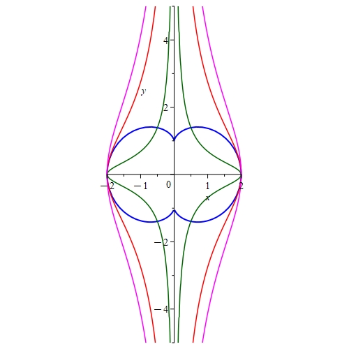
Figure 12 shows the curve for and hyperbolisms with respect to the origin and the line whose equation is for .
6 A construction of a lemniscate
The construction proposed in this section is slightly different from a hyperbolism. Studying at least one case may be an appeal to explore more cases.
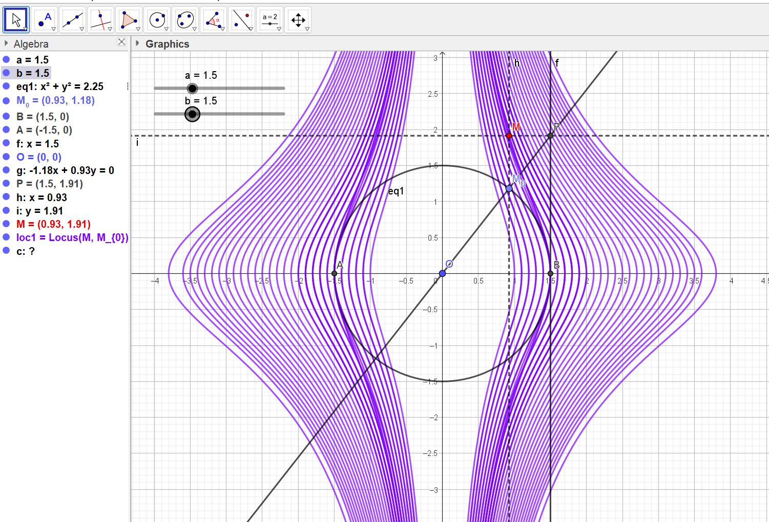
We consider a circle whose center is the origin and radius and a line whose equation is . Take a point on the circle ; the point is the intersection of with the horizontal line through . Then we define to be the point of intersection of the line with the vertical line through . The geometric locus of when runs on is a lemniscate. This is illustrated in Figure 13. The figure shows screenshots of a GeoGebra applet121212https://www.geogebra.org/m/zkgmxume; using the sliders may help to study the family of curves.
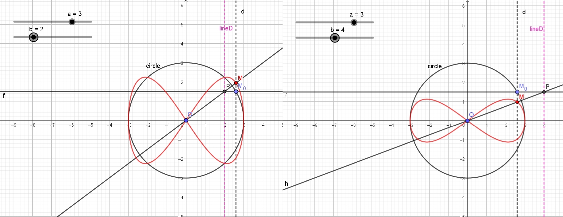
For , the lemniscate lies part out of the circle. For , the lemniscate is bounded by the circle. In both cases, the lemniscate is tangent to the circle at its vertices, i.e. its points on the axis different form the origin.
GeoGebra could not give an implicit equation for the lemniscate, we will look for such an equation via algebraic computations. We choose the same parametrization as above for the circle, i.e. the coordinates of are given by:
| (28) |
Then the coordinates of are
The equation of the line is , whence the coordinates of :
| (29) |
We apply the following code:
p1 := x*denom(xM) - numer(xM);
p2 := y*denom(yM) - numer(yM);
J := <p1, p2>;
JE := EliminationIdeal(J, {a, b, x, y});
G := Generators(JE)[1];
and obtain the polynomial
| (30) |
The vanishing set of in the real plane is called a lemniscate of Gerono.
7 Special features of the curves which have been obtained
In Section 2, the obtained hyperbolisms show common features:
-
1.
The curve has two disjoint components. On the one hand, these components cannot be distinguished by algebraic means as the defining polynomial is irreducible over the field of real numbers. This can be proven using Maple command evala(AFactor(…); the need for that command, and not the ordinary Factor command, has been analyzed in [12].
-
2.
The geometric basis of the construction induces easily that the two components are symmetric about the axis.
-
3.
From the exploration, the axis seems to be an asymptote to both. Actually, this is a consequence of the construction: when the point gets arbitrarily close to the axis, the slope of the line line, and thus coordinate of , tend to infinity.
Actually the origin does not belong to the hyperbolism of the original curve. It can be obtained only if is at the origin, but in this case the line is not defined.
8 Discussion
The 2 first examples may be treated by hand, with students having learnt an elementary course in the spirit of [2].
In this paper, we considered a question in plane geometry, which can look rather simple. Its translation using technology revealed a more complicated situation that foreseen. On the other hand, the mathematics ”behind” the screen are heavier than the general domain announced.
The problem can be understood by a regular High-School student131313Decades ago, such constructions were performed in High-School by hand using paper, pencil and ruler. Only in easy cases, an equation was derived., but the algebraic machinery beneath is then out of reach, as it belongs to Computer Algebra, and uses algorithms from Ring Theory. Moreover, we deal here with curves of higher degree than what High-School students learn, as explained in section 1.
Along the paper, implicitization has been performed using polynomial rings and elimination. Maple has an implicitize command, but we preferred to have our computations more understandable, and not to use this command as a blackbox. The user has no access to the algorithms, but via reading the paper in reference on the help page of the command. One the one hand, an educator has to make a decision between low-level and high level commands (see [13]). On the other hand, what can be done depends on the students’ theoretical background; sometimes it is necessary to use the CAS in order to bypass a lack of knowledge (see [8]).
Moreover, respective affordances of the two kinds of software that we used have been analyzed in the past, and the importance of networking between them has been emphasized [24, 25, 11]. See also [30] for the more recent developments with GeoGebra. Here the strengths of both kinds appeared sometimes different from what we were accustomed. Anyway, it is only natural that for different questions, the respective abilities and strengths of the different kinds of software which are used may vary.
Finally, the lemniscate of Gerono in Section 6 shows that classical constructions can be imitated with slight modifications and lead to software’s broader experience. After all, curiosity is the main engine for exploration and discovery.
References
References
- [1] M. Abanades, F. Botana, A. Montes, T. Recio (2014): An algebraic taxonomy for locus computation in dynamic geometry, Computer Aided Design 56, 22–33. https://doi.org/10.1016/j.cad.2014.06.008
- [2] W. Adams and P. Loustaunau (1994): An Introduction to Gröbner Bases, Graduate Studies in Mathematics 3, American Mathematical Society.
- [3] F. Botana and M. Abánades (2014). Automatic Deduction in (Dynamic) Geometry: Loci Computation, Computational Geometry 47 (1), 75-89.
- [4] J. Blazek and P. Pech (2017) Searching for loci using GeoGebra, International Journal for Technology in Mathematics Education 27, 143–147.
- [5] J.W. Bruce and P.J. Giblin (2012): Curves and Singularities, Cambridge University Press.
- [6] R. Corless, M. Giesbrecht, I. Kotsireas and S. Watt (2001). ”Numerical implicitization of parametric hypersurfaces with linear algebra.” AISC’2000 Proceedings, Madrid, Spain. LNAI 1930, Springer.
- [7] D. Cox, J. Little, D. O’Shea (1992): Ideals, Varieties, and Algorithms: An Introduction to Computational Algebraic Geometry and Commutative Algebra, Undergraduate Texts in Mathematics, NY: Springer, (1992).
- [8] Th. Dana-Picard (2005): Technology as a bypass for a lack of theoretical knowledge, International Journal of Technology in Mathematics Education 11 (3), 101-109
- [9] Th. Dana-Picard (2020). Safety zone in an entertainment park: Envelopes, offsets and a new construction of a Maltese Cross, Electronic Proceedings of the Asian Conference on Technology in Mathematics ACTM 2020, 31-50.
- [10] Th. Dana-Picard and Z. Kovács: Automated determination of isoptics with dynamic geometry, Calculemus, CICM-11 (Conference on Intelligent Computer Mathematics), RISC (Hagenberg, Austria). DOI: https://doi.org/10.13140/RG.2.2.23002.24003
- [11] Th. Dana-Picard and Z. Kovács (2021): Networking of technologies: a dialog between CAS and DGS, The electronic Journal of Mathematics and Technology (eJMT) 15 (1), 43-59, 2021.
- [12] Th. Dana-Picard and T. Recio (2023): Dynamic construction of a family of octic curves as geometric loci, AIMS Mathematics 8 (8), 19461-19476.
- [13] Th. Dana-Picard and J. Steiner (2004): The importance of “low level” CAS commands in teaching Engineering Mathematics, European Journal of Engineering Education 29 (1), 139 -146.
- [14] Th. Dana-Picard, Z. Kovács and W.-C. Yang (2023): Topology of Quartic Loci Resulted From Lines Passing through a Fixed Point and a Conic, CGTA 2023 (Conference on Geometry: Theory and Applications), Kefermarkt, Austria. DOI: https://doi.org/10.13140/RG.2.2.24291.94249
- [15] Th. Dana-Picard and T. Recio (2023): Dynamic construction of a family of octic curves as geometric loci, AIMS Mathematics 8 (8), 19461-19476.
- [16] Th. Dana-Picard and N. Zehavi (2016): Revival of a classical topic in Differential Geometry: the exploration of envelopes in a computerized environment, International Journal of Mathematical Education in Science and Technology 47(6), 938-959.
- [17] R. Duval (2018). Understanding the Mathematical Way of Thinking – The Registers of Semiotic Representations, Springer.
- [18] Ferrarello, D., Mammana, M.F., Pennisi, M., Taranto, E. (2017). Teaching Intriguing Geometric Loci with DGS. In: Aldon, G., Hitt, F., Bazzini, L., Gellert, U. (eds) Mathematics and Technology. Advances in Mathematics Education. Springer, Cham. DOI: https://doi.org/10.1007/978-3-319-51380-5_26
- [19] Ferréol, R. (2017): Piriform Quartic, https://mathcurve.com/courbes2d.gb/piriforme/piriforme.shtml (retrieved November 2024).
- [20] Ferréol, R. (2017): Hyperbolism and Antihyperbolism of a Curve - Newton Transformation, https://mathcurve.com/courbes2d.gb/hyperbolisme/hyperbolisme.shtml
- [21] G. Fischer (2001). Plane Algebraic Curves, Student Mathematical Library 15, American Mathematical Society, 2001.
- [22] X-S. Gao, S-C. Chou (1992). Implicitization of rational parametric equations, Journal of Symbolic Computation 14 (5), 459-470.https://doi.org/10.1016/0747-7171(92)90017-X
- [23] Kovács, Z.; Recio, T.; Vélez, M.P. (2022): Automated reasoning tools with GeoGebra: What are they? What are they good for?, In: P. R. Richard, M. P. Vélez, S. van Vaerenbergh (eds): Mathematics Education in the Age of Artificial Intelligence: How Artificial Intelligence can serve mathematical human learning. Series: Mathematics Education in the Digital Era, Springer,23-44. https://doi.org/10.1007/978-3-030-86909-0_2
- [24] E. Roanes-Lozano, E. Roanes-Macías, M. Villar-Mena (2003): A bridge between dynamic geometry and computer algebra, Math. Comput. Model. 37, 1005–1028. https://doi.org/10.1016/S0895-7177(03)00115-8
- [25] E. Roanes-Lozano, N. Van Labeke, E. Roanes-Macías (2010): Connecting the 3D DGS Calques3D with the CAS Maple, Mathematics and Computers in Simulation 80 (6), 1153–1176.
- [26] Sederberg, Thomas and Anderson, D.C and Goldman, Ronald (1984). Implicit representation of parametric curves and surfaces, Computer Vision, Graphics, and Image Processing 28, 72-84. DOI: https://doi.org/10.1016/0734-189X(84)90140-3
- [27] R. Sendra and F. Winkler (2008): Rational Algebraic Curves: A Computer Algebra Approach, Algorithms and Computation in Mathematics 22, Springer.
- [28] Taimina, D. (2007). Historical Mechanisms for Drawing Curves, in (Amy Shell-Gellasch, edt) Hands on History: A Resource for Teaching Mathematics, 89 - 104, Cambridge University Press. https://doi.org/10.5948/UPO9780883859766.011
- [29] D. Wang (2004). A simple method for implicitizing rational curves and surfaces, Journal of Symbolic Computation 38, 899–914.
- [30] R. Weinhandl, E. Lindenbauer, S. Schallert-Vallaster, J. Pirklbauer, M. Hohenwarter (2024). GeoGebra, a Comprehensive Tool for Learning Mathematics, in (A. Gegenfurtner and I. Kollar, edts) Designing Effective Digital Learning Environments, London: Routledge. DOI: https://doi.org/10.4324/9781003386131
- [31] Yates, R. (1947): A Handbook On Curves And Their Properties, Ann Arbor: J. Edwards.