Multivariate Distributions in Non–Stationary Complex Systems II: Empirical Results for Correlated Stock Markets

Abstract

Multivariate Distributions are needed to capture the correlation structure of complex systems. In previous works, we developed a Random Matrix Model for such correlated multivariate joint probability density functions that accounts for the non–stationarity typically found in complex systems. Here, we apply these results to the returns measured in correlated stock markets. Only the knowledge of the multivariate return distributions allows for a full–fledged risk assessment. We analyze intraday data of 479 US stocks included in the S&P500 index during the trading year of 2014. We focus particularly on the tails which are algebraic and heavy. The non–stationary fluctuations of the correlations make the tails heavier. With the few–parameter formulae of our Random Matrix Model we can describe and quantify how the empirical distributions change for varying time resolution and in the presence of non–stationarity.

1 Introduction

Global developments and ever increasing socio–economic interactions trigger the need to better understand and model complex systems [1, 2]. Large amount of high–quality data is essential for this endeavor. A wealth of data is nowadays available for financial markets making them particularly well suited to develop methods of statistical analysis and new approaches for modeling. Rare events in the tails of the distributions are especially sensitive for systemic risk and stability of a system. In financial markets, the analysis of distributions for individual stocks is of considerable importance for a variety of reasons [3, 4, 5], it is also essential to understand the mechanisms of price formation [6, 7, 8]. With globalization, the interconnectedness of the considered system must be taken into account, market–wide synchronicity and correlations of traders’ actions play a decisive role [9, 10, 11]. Univariate distributions of individual allow statements about the corresponding individual risk. Thus, the shape of those distributions is of interest [3, 4, 5]. Yet, the high correlations in financial markets imply that a univariate assessment of risk is insufficient. In recent years, such a multivariate view moved in the focus, often in the context of stochastic processes [12, 13, 14, 15, 16, 16, 17, 18, 19, 20, 21].

Another important aspect of complex systems is their non–stationarity [11, 22, 23, 24, 25]. The standard deviations or volatilities for individual returns fluctuate seemingly erratically over time [26, 27, 28, 29, 30]. The mutual dependencies such as Pearson correlations or copulas [31, 32, 33, 34, 35, 36] show non–stationarity variations as well and play a particularly important role in states of crisis [22, 37, 38, 39, 40, 41, 42, 43, 44, 45, 46, 47, 48, 49, 50, 51, 52]. The multivariate distributions, i.e. the joint probability density functions of several or even many stock returns are urgently needed to assess and understand the risks of a financial market as a whole.

To carry out a thorough empirical analysis of such multivariate distributions is our first goal. There are various ways to look at multivariate data. Here, we rotate the vector of returns into the eigenbasis of the covariance or correlation matrix. These matrices have spectra featuring a bulk as well as large eigenvalues belonging to industrial sectors and to the entire market. We obtain individual, i.e. univariate distributions for the corresponding linear combinations of returns, which provide a full picture of the multivariate data. By normalizing to the (square root of) the corresponding eigenvalue and overlaying the resulting univariate distributions we arrive at aggregated distributions of high statistical significance. We find a strong influence of non–stationarity.

Our second goal is the comparison of our results to our Random Matrix Model that we discussed in depth in Ref. [53] to which we refer as I in the sequel. It was developed in Refs. [54, 55, 56, 57, 58, 59, 60] and considerably extended in Ref. [61]. The fluctuating correlations in the non–stationary system are modeled by random matrices. The model predicts heavier tails on longer time intervals. We obtained four multivariate model distributions with heavy, mostly algebraic tails which we fit to the data. The data analyzed are well described by our algebraic multivariate return distributions. The results confirm that the non–stationary fluctuations of the correlations lift the tails.

The paper is organized as follows. In Sec. 2, we introduce our empirical data set and the procedure of aggregation. In Sec. 3, we present our empirical distributions and the fits to the model distributions. Moreover, we discuss some caveats relevant for such a large–scale data analysis in Sec. 4. We give our conclusions in Sec. 5.

2 Data and Methods of Statistical Analysis

We describe our data set in Sec. 2.1. To fix the notation and conventions, we briefly sketch the normalization of return time series and data matrices in Sec. 2.2. In Sec. 2.3, we divide long time intervals into epochs to facilitate the analysis of non–stationarity. We discuss the issue of normalization occurring in the separation of time scales. In Sec. 2.4, we briefly introduce two types of Pearson correlation matrices. Rotation and aggregation of multivariate empirical data are explained in Sec. 2.5.

2.1 Data sets

We use the Daily TAQ (Trade and Quote) of the year 2014 from the New York stock exchange (NYSE) [62]. There are different columns specified by timestamp, the bid price which is the maximum a buyer is willing to pay and the ask price which is the minimum a seller is willing to accept. As the number of used stocks is comparatively large stocks across all industrial sectors according to the Global Industry Classification Standard (GICS) [63] are represented, see App. A.1. Since the market operates in the opening and closing hours differently from its main phase, we discard the first and last 10 minutes of each day [64], i.e. we use data from 09:40 (UTC-5) until 15:50 (UTC-5). We select stocks being continually traded on every open day while simultaneously being part of the S$\&$P 500 index in 2014.

There are three days which contain artifactual data for half the day. Those three days are the 3rd of July, the 28th of November and the 24th of December, which are three public holidays on which the NYSE was only open for half a day. We remove the corresponding data but keep the normal (non–artifactual) trading data of (half) the mentioned day.

In addition to the aforementioned data set that we use for our analyses in Secs. 2.5 and 3, we select a second one similar to the data set from Refs. [54, 65] to discuss carefully further aspects of our analysis, see Sec. 4.2. The data set has a daily time resolution with stocks that were listed in the S&P 500 index, see App. A.2. In total, it comprises 308 stocks for a time period ranging from January 23, 1992 to December 31, 2012. This data set lists daily adjusted prices.

2.2 Normalization of returns

Our data contain stock $K$ stocks which we label as $k=1,\ldots,K$. In our analysis, we include $K=479$ stocks. For our analysis in Sec. 3, we derive the observables from the midpoint price as it allows analyses with higher time resolutions compared to stock prices. Importantly, the dynamics of prices and midpoints is comparable. With best ask $a_{k}(t)$ and best bid $b_{k}(t)$ the midpoint price reads

$$m_{k}(t)=\frac{a_{k}(t)+b_{k}(t)}{2}\ ,\hskip 28.45274ptk=1,\ldots,K\ .$$ (II.1)

From the midpoint price, we calculate the logarithmic returns

$$G_{k}(t)=\ln\frac{m_{k}(t+\Delta t)}{m_{k}(t)}\ ,\hskip 28.45274ptk=1,\ldots,K\ .$$ (II.2)

which depend on the chosen return horizon $\Delta t$. We arrange the return time series $G_{k}(t),t=1,\ldots,T$, as the rows of the $K\times T$ data matrix

$$G=\left[\begin{array}[]{ccccc}G_{1}(1)&\cdots&G_{1}(t)&\cdots&G_{1}(T)\\ \vdots&\vdots&\vdots&\vdots&\vdots\\ G_{k}(1)&\cdots&G_{k}(t)&\cdots&G_{k}(T)\\ \vdots&\vdots&\vdots&\vdots&\vdots\\ G_{K}(1)&\cdots&G_{K}(t)&\cdots&G_{K}(T)\end{array}\right]\ .$$ (II.3)

We normalize of each row in Eq. (II.3) to zero mean and unit standard deviation which yields the time series

$$\mathcal{M}_{k}(t)=\frac{G_{k}(t)-\langle G_{k}(t)\rangle_{T}}{\sigma_{k}}\ ,\hskip 28.45274ptk=1,\ldots,K\ .$$ (II.4)

The sample average is defined as

$$\langle f_{k}(t)\rangle_{T}=\frac{1}{T}\sum_{t=1}^{T}f_{k}(t)\ ,$$ (II.5)

such that $\langle G_{k}(t)\rangle$ is the sample mean and

$$\sigma_{k}=\sqrt{\langle\left(G_{k}(t)-\langle G_{k}(t)\rangle_{T}\right)^{2}\rangle_{T}}\,.$$ (II.6)

the sample standard deviation. The resulting $K\times T$ data matrix $\mathcal{M}$ contains the normalized return time series $\mathcal{M}_{k}(t),\ t=1,\ldots,T$, as rows.

We may also normalize the columns of $G$ to zero mean and unit standard deviation $\varrho(t)$. This yields a different type of series in the index $k$, referred to as position series,

$$\mathcal{E}_{k}(t)=\frac{G_{k}(t)-\langle G_{k}(t)\rangle_{K}}{\varrho(t)}$$ (II.7)

with the sample average

$$\langle f_{k}(t)\rangle_{K}=\frac{1}{K}\sum_{k=1}^{K}f_{k}(t)\,.$$ (II.8)

The resulting $K\times T$ data matrix $\mathcal{E}$ contains as columns the normalized return position series $\mathcal{E}_{k}(t),\ k=1,\ldots,K$. Time series provide information on subsequent events in one stock or, more generally, position $k$, while position time series collect the information on all positions at a given time $t$.

2.3 Epochs and long interval

We consider the trading year 2014 with a total of $250$ trading days. To analyze non–stationarity, we separate time scales by dividing the long time interval into many small ones, referred to as epochs as shown in Fig. 1. Anticipating the later discussion, one can try to choose the epoch length such that the effects of non–stationarity are negligible or at least much smaller than across epochs, i.e. on the long time interval. Nevertheless, conceptually this is not a prerequisite for applying our model. For the data under consideration, it turns out reasonable to choose one trading day as epoch length. The longer interval can be one trading year, such that 25 trading days correspond to ten intervals or 50 trading days to five intervals for the whole year, see App. B.1.

Importantly, we calculate the data matrices for the returns separately for each epoch and concatenate those together to obtain the return data matrix for a longer interval, see Sec. 4.2.

Figure 1: Division of the whole year 2014 into epochs and long intervals.

We carry out our analysis for different time resolutions, i. e. $\Delta t=1\,\mathrm{s}$ and $\Delta t=10\,\mathrm{s}$. These two considered return horizons limit the number of data points $T$ that can be chosen for an epoch and for the long interval in our analysis. The number of data points are 22200 per epoch ($\Delta t=1\,\mathrm{s}$) and 2220 per epoch ($\Delta t=10\,\mathrm{s}$). It is very important that we normalize our time series to the considered epoch or interval, see Eq. (II.4).

2.4 Two types of correlation matrices

Since we introduced time and position series, there are two different Pearson correlation matrices. Using the data matrix $\mathcal{M}$, we have the $K\times K$ correlation matrix of the time series

$$C=\frac{1}{T}\mathcal{M}\mathcal{M}^{\dagger}\ ,$$ (II.9)

where we employ $\dagger$ to denote the transpose of a matrix. Here, $T$ stands for the number of data points in either the long interval or in epochs. In the sequel, the sample correlation matrices on the long interval and in the epochs will be denoted $C_{\mathrm{ep}}$ and $C$, respectively. Using the data matrix $\mathcal{E}$, we find the $T\times T$ correlation matrix of the position series matrix,

$$D=\frac{1}{K}\mathcal{E}^{\dagger}\mathcal{E}\ .$$ (II.10)

While $C$ measures the relations between the different stocks, $D$ captures the dependencies in time, i.e. the non–Markovian features. Contrary to some confusing remarks in the literature, $C$ and $D$ are not equivalent. Due to the different normalizations of time and position series, eigenvalues and eigenvectors differ.

2.5 Rotation and aggregation of empirical data

In Eq. (II.4) we introduced the notation $\mathcal{M}_{k}(t)$ for the returns that is then used to calculate the correlation matrices $C_{\mathrm{ep}}$ or $C$. As we wish to analyze multivariate return distributions, it is advised to employ another notation for the returns if they appear as arguments of the distributions, we choose the notation $r_{k}(t)$ such that $r(t)=(r_{1}(t),\ldots,r_{K}(t))$ is the $K$ component vector of returns at a given time $t$. In the sequel, we will simply write $r$, because the steps taken are the same for all times $t$. We recall that the returns $r$ are always normalized on the considered epoch or on the long time interval. As the correlation matrices are real symmetric, all eigenvalues are real. Due to the specific form (II.9), the eigenvalues of a correlation matrix are positive semidefinite, in our case positive definite, since we always work with correlation matrices of full rank. As in the theoretical discussion in I, we diagonalize

$$C=U\Lambda U^{\dagger}\qquad\mathrm{with}\qquad\Lambda=\mathrm{diag}(\Lambda_{1},\ldots,\Lambda_{K})\ ,\quad\Lambda_{k}>0$$ (II.11)

with an an orthogonal matrix $U$. The same applies to $C_{\mathrm{ep}}$ with eigenvalues $\Lambda_{\mathrm{ep},k}$. For the inverse correlation matrices, we then have $C^{-1}=U\Lambda^{-1}U^{\dagger}$. As we work with full–rank correlation matrices, the existence of their inverse is warranted. For the squared Mahalanobis distance [66] we have

$$r^{\dagger}C^{-1}r=r^{\dagger}U=\sum_{k=1}^{K}\frac{\bar{r}_{k}^{2}}{\Lambda_{k}}\qquad\mathrm{with}\qquad\bar{r}_{k}=\sum_{l=1}^{K}U_{lk}r_{l}\ ,$$ (II.12)

see I, and similarly for $C_{\mathrm{ep}}$. The linear combinations $\bar{r}_{k}$, are the returns rotated into the eigenbasis of the correlation or covariance, respectively, matrix.

By sampling, we then work out the empirical univariate distributions $p^{(\mathrm{rot},k)}(\bar{r}_{k})$ of the rotated returns $\bar{r}_{k}$. These $K$ distributions provide full information on the multivariate system, because all linear combinations differ. To accumulate statistics, we can normalize to the square root of the corresponding eigenvalue,

$$\widetilde{r}_{k}=\frac{\bar{r}_{k}}{\sqrt{\Lambda_{k}}},$$ (II.13)

or $\Lambda_{\mathrm{ep},k}$, respectively, and lump together all $K$ distributions. We refer to this averaging procedure as aggregation. It yields a statistically highly significant univariate empirical distribution which facilitates a careful study of the tail behavior.

Figure 2 shows the univariate distributions of the rotated returns $p^{(\mathrm{rot},k)}(\bar{r}_{k})$ derived from the Daily TAQ data set with $\Delta t=1\,\mathrm{s}$, see Sec. 2.1.

\begin{overpic}[width=368.57964pt]{Images/Year2014_RotationRet_AllEigenval1stLargest2ndLargestkthRow.pdf} \put(50.0,2.0){\makebox(0.0,0.0)[]{\large rotated return}} \put(1.0,35.0){\makebox(0.0,0.0)[]{\rotatebox{90.0}{\large pdf}}} \end{overpic}

Figure 2: Empirical distributions of the rotated returns $p^{(\mathrm{rot},k)}(\bar{r}_{k})$ for the whole year of 2014 with $\Delta t=1\,\mathrm{s}$. Distributions corresponding to the largest eigenvalue (blue) and second largest eigenvalue (red) are highlighted.

\begin{overpic}[width=368.57964pt]{Images/Year2014_RotationRet_+10Largest-version2.pdf} \put(50.0,2.0){\makebox(0.0,0.0)[]{\large rotated return}} \put(1.0,35.0){\makebox(0.0,0.0)[]{\rotatebox{90.0}{\large pdf}}} \end{overpic}

Figure 3: Empirical distributions of the rotated returns $p^{(\mathrm{rot})}(\bar{r}_{k})$ corresponding to the ten largest eigenvalues for the whole year of 2014 with $\Delta t=1\,\mathrm{s}$. Distributions corresponding to the largest eigenvalue (blue) and second largest eigenvalue (red) are highlighted.

\begin{overpic}[width=368.57964pt]{Images/Year2014_RotationRet_+10Smallest-version2.pdf} \put(50.0,2.0){\makebox(0.0,0.0)[]{\large rotated return}} \put(1.0,35.0){\makebox(0.0,0.0)[]{\rotatebox{90.0}{\large pdf}}} \end{overpic}

Figure 4: Empirical distributions of the rotated returns $p^{(\mathrm{rot})}(\bar{r}_{k})$ distributions corresponding to the ten smallest eigenvalues for the whole year of 2014 with $\Delta t=1\,\mathrm{s}$.

\begin{overpic}[width=368.57964pt]{Images/FigCorrMatSpectrum_2014.pdf} \put(70.0,51.0){\Large market} \put(76.0,50.0){\color[rgb]{0,0,1}\vector(1,-1){10.0}} \put(36.0,17.0){\Large industrial sectors} \put(26.0,12.0){\makebox(52.0,5.0)[]{{\color[rgb]{0,0,1}\downbracefill}}} \put(30.0,55.0){\Large bulk} \put(30.0,54.0){\color[rgb]{0,0,1}\vector(-1,-1){9.1}} \put(25.0,36.0){\Large small eigenvalues} \put(30.0,35.0){\color[rgb]{0,0,1}\vector(0,-1){14.5}} \put(50.0,2.0){\makebox(0.0,0.0)[]{\large eigenvalue}} \put(5.0,35.0){\makebox(0.0,0.0)[]{\rotatebox{90.0}{\large pdf}}} \end{overpic}

Figure 5: Spectrum of correlation matrix for the whole year of 2014 with $K=479$ stocks with $\Delta t=1\,\mathrm{s}$.

To zoom into the details, the distributions of the rotated returns corresponding to the largest ten and smallest eigenvalues are depicted in Figs. 3 and 4, respectively. Anticipating the later discussion, an important remark is in order. It is well–known that the spectra of large financial correlation or covariance matrices consist of a rather universal bulk and of outliers which are due to the industrial sectors, the largest one captures the collective motion of the market as a whole [11], see Fig. 5. Even the smallest eigenvalues can separate from the bulk eigenvalues. As expected the univariate distributions of the rotated returns in Fig. 3 corresponding to the ten largest outliers differ from those corresponding to the bulk eigenvalues and thus carry important additional information. Moreover, the distributions corresponding to the largest and second largest eigenvalues are heavier-tailed than the distributions corresponding to the bulk eigenvalues. For the distributions of the rotated returns corresponding to the smallest eigenvalues in Fig. 4, we observe stronger oscillations presumably caused by the discrete nature of the prices due to the tick size [67].

For comparison, it is also instructive to work out the univariate distributions of the normalized, original (unrotated) returns $p^{(\mathrm{orig},k)}(r_{k})$.

\begin{overpic}[width=368.57964pt]{Images/Year2014_NormalizedOriginalRet_TROW.pdf} \put(50.0,2.0){\makebox(0.0,0.0)[]{\large original return}} \put(1.0,35.0){\makebox(0.0,0.0)[]{\rotatebox{90.0}{\large pdf}}} \end{overpic}

Figure 6: Empirical distribution of the normalized, original returns $p^{(\mathrm{orig},k)}(r_{k})$ for the whole year 2014 with $\Delta t=1\,\mathrm{s}$ for stock T. Rowe Price (TROW).

\begin{overpic}[width=368.57964pt]{Images/Year2014_NormalizedOriginalRet.pdf} \put(50.0,2.0){\makebox(0.0,0.0)[]{\large original return}} \put(1.0,35.0){\makebox(0.0,0.0)[]{\rotatebox{90.0}{\large pdf}}} \end{overpic}

Figure 7: Empirical distributions of the normalized, original returns $p^{(\mathrm{orig},k)}(r_{k})$ for all stocks $k=1,\ldots,K$ with $K=479$ for the whole year 2014 with $\Delta t=1\,\mathrm{s}$.

We show a single typical return distribution for a time resolution of $\Delta t=1\,\mathrm{s}$ in Fig. 6. Surprisingly, deep dips give it a fence–like appearance. This shape of the distribution can also be traced back to the tick size as smallest trading unit [67]. Analogous to Fig. 2, we display all $k=1,\ldots,K$, univariate distributions of the normalized, original returns together in Fig. 7. Apart from this very peculiar feature of the univariate distributions for the original returns, it becomes obvious that the univariate distributions for the rotated returns carry much more information, namely on the correlation structure. They depend on the corresponding eigenvalue with a strong influence on the shapes, as see in Figs. 2–4.

3 Comparison of the multivariate model distributions with the data

In Sec. 3.1, we briefly review the process of aggregation and discuss the model distributions for the aggregated empirical ones. In Sec. 3.2, we determine the fit parameters for the epoch distributions of the aggregated returns. Based on the determination of these values, we fit the distributions of the aggregated returns on the long intervals in Sec. 3.3. In Sec. 3.4, we show that these distributions on the long intervals indeed have a stronger tail behavior caused by the fluctuations of the correlation matrices. Furthermore, we take a closer look at the tails in the distributions of the aggregated returns in Sec. 3.5.

3.1 Aggregating the Return Distributions

In Sec. LABEL:I,subsec:agg, we introduced the univariate distributions of the rotated returns. To obtain better statistics for larger return horizon $\Delta t$ we go over to the distributions $p^{(\mathrm{aggr})}(\widetilde{r})$ of the aggregated returns (II.13). This rescaling with the corresponding eigenvalues moves the empirical, univariate distributions of the rotated, unrescaled returns, see Fig. 2, corresponding to different eigenvalues closer together, see Fig. 8.

\begin{overpic}[width=368.57964pt]{Images/Year2014_AggregRet_ALL+1Largest+2Largest.pdf} \put(52.0,0.0){\makebox(0.0,0.0)[]{\large aggregated return}} \put(2.0,35.0){\makebox(0.0,0.0)[]{\rotatebox{90.0}{\large pdf}}} \put(75.0,55.0){\makebox(0.0,0.0)[]{}} \end{overpic}

Figure 8: Empirical distribution of the aggregated returns $p^{(\mathrm{aggr})}(\widetilde{r})$ for the whole year 2014 with $\Delta t=1\,\mathrm{s}$ (black). Empirical distribution $p^{(\mathrm{rot,scal},k)}(\widetilde{r}_{k})$ corresponding to the largest eigenvalue for $k=K$ is displayed in blue color and for second largest eigenvalue for $k=K-1$ in red color.

However, the empirical distributions $p^{(\mathrm{rot,scal},k)}(\widetilde{r}_{k})$ of the rotated and rescaled returns corresponding to the largest and second largest eigenvalues for $k=K$ and $k=K-1$, respectively, are still heavier–tailed than the empirical aggregated distribution of all returns $p^{(\mathrm{aggr})}(\widetilde{r})$. The situation is reminiscent of other statistical situations where one has a null hypothesis as for example in the case of the Marchenko–-Pastur distribution [68]. Here, the distribution of the aggregated returns is the null hypothesis.

In the sequel, we analogously transform the model distribution  (LABEL:I,eq:RotRescAlgebraic) for the epochs and those for the long interval (LABEL:I,eqn:RotRescPGG), (LABEL:I,eqn:RotRescPGA_New), (LABEL:I,eqn:RotRescPAG_New) and (LABEL:I,eqn:RotRescPAA_New) of the rotated returns into distributions of the rotated and rescaled returns. In the formulae, this is done by replacing the eigenvalues $\Lambda_{k}$ with one, as the functional forms of the distributions is the same for all $k$ in the respective model.

3.2 Fits of the aggregated empirical distributions on epochs

When looking at heavy–tailed distributions, one is usually interested in their shapes on two scales, the linear one that emphasizes the region around zero, and the logarithmic one that allows an assessment of the tail–behavior. Thus, we carry out two least square fits for each distributions, a linear and a logarithmic one. We use the normalized $\chi^{2}_{\mathrm{lin}}$ and $\chi^{2}_{\mathrm{ln}}$ [69] as measures for the goodness of the fit.

For two selected epochs, the 8th of December and the 17th of December, we show in Figs. 9 and 10 empirical distributions $p^{(\mathrm{aggr})}(\widetilde{r})$ of the aggregated returns with fits on a logarithmic and a linear scale for $\Delta t=1\,\mathrm{s}$. For $\Delta t=10\,\mathrm{s}$, the same comparisons are depicted in Figs. 11 and 12 for the 20th of December and the 2nd of June, respectively. As expected for intraday data the empirical distributions have strong heavy tails. For a smaller return horizon $\Delta t$, the distributions are heavier–tailed and the distributions shows a higher probability near their centers [5, 70]. For these four different epochs, we obtain very good fits for the distributions of the aggregated returns $p_{\mathrm{A}}^{(\mathrm{aggr})}(\widetilde{r})$. The model parameter $l_{\mathrm{rot}}$ and the fit parameter are listed in App. B.2. Furthermore, we notice that the fit parameters change due to the non-stationarity of the epoch distributions.

By averaging over all fit parameters $l_{\mathrm{rot}}$ for all epoch distributions in 2014, we determine the parameter $\langle l_{\mathrm{rot}}\rangle$ as input for the upcoming discussion of the distributions on the long interval, see App. B.3. The parameters vary for different return horizons $\Delta t$ and also for linear or logarithmic fits.

\begin{overpic}[width=433.62pt]{Images/Fit_22200_DistEpoch_pA_Log_20141208.pdf} \put(18.0,55.0){\noindent\framebox{\parbox{42.67912pt}{Dec 8\\ $\mathsf{\Delta t=1\,s}$}}} \put(50.0,0.0){\makebox(0.0,0.0)[]{\small aggregated return}} \put(2.0,35.0){\makebox(0.0,0.0)[]{\rotatebox{90.0}{\small pdf}}} \put(78.0,55.0){\makebox(0.0,0.0)[]{\Large A}} \end{overpic}

(a)

\begin{overpic}[width=433.62pt]{Images/Fit_22200_DistEpoch_pA_Lin_20141208.pdf} \put(18.0,55.0){\noindent\framebox{\parbox{42.67912pt}{Dec 8\\ $\mathsf{\Delta t=1\,s}$}}} \put(50.0,0.0){\makebox(0.0,0.0)[]{\small aggregated return}} \put(2.0,35.0){\makebox(0.0,0.0)[]{\rotatebox{90.0}{\small pdf}}} \put(78.0,55.0){\makebox(0.0,0.0)[]{\Large A}} \end{overpic}

(b)

Figure 9: Empirical distributions of aggregated returns with $\Delta t=1\,\mathrm{s}$ (black) for epoch December 8, 2014 with $p_{\mathrm{A}}^{(\mathrm{aggr})}(\widetilde{r})$ (red circles), left: for $l_{\mathrm{rot}}=2.936$ on a logarithmic scale, right: for $l_{\mathrm{rot}}=2.742$ on a linear scale.

\begin{overpic}[width=433.62pt]{Images/Fit_22200_DistEpoch_pA_Log_20141217.pdf} \put(18.0,55.0){\noindent\framebox{\parbox{42.67912pt}{Dec 17\\ $\mathsf{\Delta t=1\,s}$}}} \put(50.0,0.0){\makebox(0.0,0.0)[]{\small aggregated return}} \put(2.0,35.0){\makebox(0.0,0.0)[]{\rotatebox{90.0}{\small pdf}}} \put(78.0,55.0){\makebox(0.0,0.0)[]{\Large A}} \end{overpic}

(a)

\begin{overpic}[width=433.62pt]{Images/Fit_22200_DistEpoch_pA_Lin_20141217.pdf} \put(18.0,55.0){\noindent\framebox{\parbox{42.67912pt}{Dec 17\\ $\mathsf{\Delta t=1\,s}$}}} \put(50.0,0.0){\makebox(0.0,0.0)[]{\small aggregated return}} \put(2.0,35.0){\makebox(0.0,0.0)[]{\rotatebox{90.0}{\small pdf}}} \put(78.0,55.0){\makebox(0.0,0.0)[]{\Large A}} \end{overpic}

(b)

Figure 10: Empirical distributions of aggregated returns with $\Delta t=1\,\mathrm{s}$ (black) for epoch December 17, 2014 with $p_{\mathrm{A}}^{(\mathrm{aggr})}(\widetilde{r})$ (red circles), left: for $l_{\mathrm{rot}}=2.688$ on a logarithmic scale, right: for $l_{\mathrm{rot}}=2.351$ on a linear scale.

\begin{overpic}[width=390.25534pt]{Images/Fit_2220_DistEpoch_pA_Log_20140220.pdf} \put(18.0,55.0){\noindent\framebox{\parbox{48.36958pt}{Feb 20\\ $\mathsf{\Delta t=10\,s}$}}} \put(50.0,0.0){\makebox(0.0,0.0)[]{\small aggregated return}} \put(2.0,35.0){\makebox(0.0,0.0)[]{\rotatebox{90.0}{\small pdf}}} \put(78.0,55.0){\makebox(0.0,0.0)[]{\Large A}} \end{overpic}

(a)

\begin{overpic}[width=390.25534pt]{Images/Fit_2220_DistEpoch_pA_Lin_20140220.pdf} \put(18.0,55.0){\noindent\framebox{\parbox{48.36958pt}{Feb 20\\ $\mathsf{\Delta t=10\,s}$}}} \put(50.0,0.0){\makebox(0.0,0.0)[]{\small aggregated return}} \put(2.0,35.0){\makebox(0.0,0.0)[]{\rotatebox{90.0}{\small pdf}}} \put(78.0,55.0){\makebox(0.0,0.0)[]{\Large A}} \end{overpic}

(b)

Figure 11: Empirical distributions of aggregated returns with $\Delta t=10\,\mathrm{s}$ (black) for epoch February 20, 2014 with $p_{\mathrm{A}}^{(\mathrm{aggr})}(\widetilde{r})$ (red circles), left: for $l_{\mathrm{rot}}=3.217$ on a logarithmic scale, right: for $l_{\mathrm{rot}}=3.108$ on a linear scale.

\begin{overpic}[width=433.62pt]{Images/Fit_2220_DistEpoch_pA_Log_20140602.pdf} \put(18.0,55.0){\noindent\framebox{\parbox{48.36958pt}{Jun 2\\ $\mathsf{\Delta t=10\,s}$}}} \put(50.0,0.0){\makebox(0.0,0.0)[]{\small aggregated return}} \put(2.0,35.0){\makebox(0.0,0.0)[]{\rotatebox{90.0}{\small pdf}}} \put(78.0,55.0){\makebox(0.0,0.0)[]{\Large A}} \end{overpic}

(a)

\begin{overpic}[width=433.62pt]{Images/Fit_2220_DistEpoch_pA_Lin_20140602.pdf} \put(18.0,55.0){\noindent\framebox{\parbox{48.36958pt}{Jun 2\\ $\mathsf{\Delta t=10\,s}$}}} \put(50.0,0.0){\makebox(0.0,0.0)[]{\small aggregated return}} \put(2.0,35.0){\makebox(0.0,0.0)[]{\rotatebox{90.0}{\small pdf}}} \put(78.0,55.0){\makebox(0.0,0.0)[]{\Large A}} \end{overpic}

(b)

Figure 12: Empirical distributions of aggregated returns with $\Delta t=10\,\mathrm{s}$ (black) for epoch June 02, 2014 with $p_{\mathrm{A}}^{(\mathrm{aggr})}(\widetilde{r})$ (red circles), left: for $l_{\mathrm{rot}}=3.249$ on a logarithmic scale, right: for $l_{\mathrm{rot}}=3.008$ on a linear scale.

3.3 Fits of the aggregated distributions on the long interval

For all four model distributions on the long interval, we insert the averaged values $\langle l_{\mathrm{rot}}\rangle$ which are between 2 and 4, see App. B.3. By fitting, we determine the remaining parameters $N$ and $L_{\mathrm{rot}}$. Figures 13– 15 display the empirical distributions of the aggregated returns and the corresponding fits on an interval of 25 trading days. We show the fits for all four model distributions in Figs. 13 and 14 for a long interval ranging from the 17th of October to the 20th of November. For both return horizons $\Delta t=1\,\mathrm{s}$ and $\Delta t=10\,\mathrm{s}$, the fits for $\langle p\rangle_{\mathrm{GA}}^{(\mathrm{aggr})}(\widetilde{r})$, $\langle p\rangle_{\mathrm{AG}}^{(\mathrm{aggr})}(\widetilde{r})$ and $\langle p\rangle_{\mathrm{AA}}^{(\mathrm{aggr})}(\widetilde{r})$ outperform the one for $\langle p\rangle_{\mathrm{GG}}^{(\mathrm{aggr})}(\widetilde{r})$. The corresponding fit parameters are listed in App. B.4. Visually, there are hardly any differences between the three better fits, Gaussian-Algebraic performs slightly better than Algebraic-Gaussian and Algebraic-Algebraic on logarithmic and linear scale, see the parameters in App. B.5. Analogous to App. 3.2, the distributions are heavier-tailed and the distributions show a higher probability near their centers for a smaller return horizon. To be consistent in our modeling, we must exclude the Gaussian–Gaussian and the Gaussian–Algebraic cases as we confirmed the validity of the algebraic distribution in the epochs. The Algebraic–Gaussian and Algebraic–Algebaic model distributions perform almost equally well. However, the Algebraic–Algebraic case seems to be slightly favored, we proceed with that choice in the sequel. The fit parameters tend to be larger for a larger return horizon $\Delta t$, see App. B.4. This observation is consistent with Ref. [54] where the Gaussian-Gaussian case was discussed for the fit parameter $N$ which increases for a larger return horizon $\Delta t$. An exception is $L_{\mathrm{rot}}$ for the Algebraic-Algebraic case which decreases for a larger return horizon.

Analogous to the fits on the longer interval of 25 trading days, we also study the empirical distributions of the aggregated returns on a longer interval of 50 trading days, as displayed Figs. 16–17. Qualitatively, the results for this interval length are similar to those for 25 trading days. By averaging all values for a specified fit scale, a fixed return horizon $\Delta t$ and a fixed interval length, we notice a trend. A larger long interval results in a smaller fit parameters for $N$ and $L_{\mathrm{rot}}$. However, the smaller $N$ and $L_{\mathrm{rot}}$ are, the stronger are the fluctuations of correlations and the heavier are the tails. The fit parameters are listed in App. C.

3.4 Comparing the shapes of the distributions on the epochs and on the long interval

We want to demonstrate that distributions of the aggregated returns on longer intervals are heavier–tailed than on shorter ones. To this end, we overlay in Fig. 18 the 250 model distributions $p_{\mathrm{A}}^{(\mathrm{aggr})}(\widetilde{r})$ calculated with the fit parameters for each epoch with the model distribution $\langle p\rangle_{\mathrm{AA}}^{(\mathrm{aggr})}(\widetilde{r})$ from the first long interval for 25 trading days with $\Delta t=1\,\mathrm{s}$. Indeed, the latter one is heavier-tailed than all 250 model distributions on the epochs.

Similarly, we compare the model distributions for the Algebraic–Algebraic case on intervals of 25 and 50 trading days in Fig. 19. We notice that the model distributions on 50 trading day intervals are heavier–tailed. When going from the one–day epochs to the long interval of 25 days, the differences in the distributions are larger as there is a factor of 25 between the lengths of the considered intervals. Here, there is only a factor of two. These results strongly corroborate our model assumption that the fluctuations of the correlation matrices make the tails heavier the longer the considered interval.

\begin{overpic}[width=433.62pt]{Images/Fit_22200_DistInt_pGG_Log_Interval_9.pdf} \put(18.0,55.0){\noindent\framebox{\parbox{42.67912pt}{25 days\\ $\mathsf{\Delta t=1\,s}$}}} \put(50.0,0.0){\makebox(0.0,0.0)[]{\small aggregated return}} \put(2.0,35.0){\makebox(0.0,0.0)[]{\rotatebox{90.0}{\small pdf}}} \put(78.0,55.0){\makebox(0.0,0.0)[]{\Large GG}} \end{overpic}

(a)

\begin{overpic}[width=433.62pt]{Images/Fit_22200_DistInt_pGA_Log_Interval_9.pdf} \put(18.0,55.0){\noindent\framebox{\parbox{42.67912pt}{25 days\\ $\mathsf{\Delta t=1\,s}$}}} \put(50.0,0.0){\makebox(0.0,0.0)[]{\small aggregated return}} \put(2.0,35.0){\makebox(0.0,0.0)[]{\rotatebox{90.0}{\small pdf}}} \put(78.0,55.0){\makebox(0.0,0.0)[]{\Large GA}} \end{overpic}

(b)

\begin{overpic}[width=433.62pt]{Images/Fit_22200_DistInt_pAG_Log_Interval_9.pdf} \put(18.0,55.0){\noindent\framebox{\parbox{42.67912pt}{25 days\\ $\mathsf{\Delta t=1\,s}$}}} \put(50.0,0.0){\makebox(0.0,0.0)[]{\small aggregated return}} \put(2.0,35.0){\makebox(0.0,0.0)[]{\rotatebox{90.0}{\small pdf}}} \put(78.0,55.0){\makebox(0.0,0.0)[]{\Large AG}} \end{overpic}

(c)

\begin{overpic}[width=433.62pt]{Images/Fit_22200_DistInt_pAA_Log_Interval_9.pdf} \put(18.0,55.0){\noindent\framebox{\parbox{42.67912pt}{25 days\\ $\mathsf{\Delta t=1\,s}$}}} \put(50.0,0.0){\makebox(0.0,0.0)[]{\small aggregated return}} \put(2.0,35.0){\makebox(0.0,0.0)[]{\rotatebox{90.0}{\small pdf}}} \put(78.0,55.0){\makebox(0.0,0.0)[]{\Large AA}} \end{overpic}

(d)

Figure 13: Empirical distributions of aggregated returns with $\Delta t=1\,\mathrm{s}$ (black) for the 9th long interval (25 trading days) on a logarithmic scale. Model distributions in red color with Gaussian–Gaussian: $N=0.794$, Gaussian–Algebraic: $L_{\mathrm{rot}}=3.466$, $N=2.436$, Algebraic–Gaussian: $N=2.848$, Algebraic–Algebraic: $L_{\mathrm{rot}}=99.551$, $N=2.906$.

\begin{overpic}[width=433.62pt]{Images/Fit_22200_DistInt_pGG_Lin_Interval_9.pdf} \put(18.0,55.0){\noindent\framebox{\parbox{42.67912pt}{25 days\\ $\mathsf{\Delta t=1\,s}$}}} \put(50.0,0.0){\makebox(0.0,0.0)[]{\small aggregated return}} \put(2.0,35.0){\makebox(0.0,0.0)[]{\rotatebox{90.0}{\small pdf}}} \put(78.0,55.0){\makebox(0.0,0.0)[]{\Large GG}} \end{overpic}

(a)

\begin{overpic}[width=433.62pt]{Images/Fit_22200_DistInt_pGA_Lin_Interval_9.pdf} \put(18.0,55.0){\noindent\framebox{\parbox{42.67912pt}{25 days\\ $\mathsf{\Delta t=1\,s}$}}} \put(50.0,0.0){\makebox(0.0,0.0)[]{\small aggregated return}} \put(2.0,35.0){\makebox(0.0,0.0)[]{\rotatebox{90.0}{\small pdf}}} \put(78.0,55.0){\makebox(0.0,0.0)[]{\Large GA}} \end{overpic}

(b)

\begin{overpic}[width=433.62pt]{Images/Fit_22200_DistInt_pAG_Lin_Interval_9.pdf} \put(18.0,55.0){\noindent\framebox{\parbox{42.67912pt}{25 days\\ $\mathsf{\Delta t=1\,s}$}}} \put(50.0,0.0){\makebox(0.0,0.0)[]{\small aggregated return}} \put(2.0,35.0){\makebox(0.0,0.0)[]{\rotatebox{90.0}{\small pdf}}} \put(78.0,55.0){\makebox(0.0,0.0)[]{\Large AG}} \end{overpic}

(c)

\begin{overpic}[width=433.62pt]{Images/Fit_22200_DistInt_pAA_Lin_Interval_9.pdf} \put(18.0,55.0){\noindent\framebox{\parbox{42.67912pt}{25 days\\ $\mathsf{\Delta t=1\,s}$}}} \put(50.0,0.0){\makebox(0.0,0.0)[]{\small aggregated return}} \put(2.0,35.0){\makebox(0.0,0.0)[]{\rotatebox{90.0}{\small pdf}}} \put(78.0,55.0){\makebox(0.0,0.0)[]{\Large AA}} \end{overpic}

(d)

Figure 14: Empirical distributions of aggregated returns with $\Delta t=1\,\mathrm{s}$ (black) for the 9th long interval (25 trading days) on a linear scale. Model distributions in red color with Gaussian–Gaussian: $N=2.038$, Gaussian–Algebraic: $L_{\mathrm{rot}}=4.425$, $N=5.078$, Algebraic–Gaussian: $N=5.986$, Algebraic–Algebraic: $L_{\mathrm{rot}}=100.355$, $N=6.149$.

\begin{overpic}[width=433.62pt]{Images/Fit_2220_DistInt_pAA_Log_Interval_8.pdf} \put(18.0,55.0){\noindent\framebox{\parbox{48.36958pt}{25 days\\ $\mathsf{\Delta t=10\,s}$}}} \put(50.0,0.0){\makebox(0.0,0.0)[]{\small aggregated return}} \put(2.0,35.0){\makebox(0.0,0.0)[]{\rotatebox{90.0}{\small pdf}}} \put(78.0,55.0){\makebox(0.0,0.0)[]{\Large AA}} \end{overpic}

(a)

\begin{overpic}[width=433.62pt]{Images/Fit_2220_DistInt_pAA_Lin_Interval_8.pdf} \put(18.0,55.0){\noindent\framebox{\parbox{48.36958pt}{25 days\\ $\mathsf{\Delta t=10\,s}$}}} \put(50.0,0.0){\makebox(0.0,0.0)[]{\small aggregated return}} \put(2.0,35.0){\makebox(0.0,0.0)[]{\rotatebox{90.0}{\small pdf}}} \put(78.0,55.0){\makebox(0.0,0.0)[]{\Large AA}} \end{overpic}

(b)

Figure 15: Empirical distributions of aggregated returns with $\Delta t=10\,\mathrm{s}$ (black) for the 8th long interval (25 trading days) with $\langle p\rangle_{\mathrm{AA}}^{(\mathrm{aggr})}(\widetilde{r})$ (red circles), left: for $L_{\mathrm{rot}}=11.032$, $N=10.031$ on a logarithmic scale, right: for $L_{\mathrm{rot}}=13.562$, $N=19.029$ on linear scale.

\begin{overpic}[width=433.62pt]{Images/Fit_50TD_22200_DistInt_pAA_Log_Interval_1.pdf} \put(18.0,55.0){\noindent\framebox{\parbox{48.36958pt}{50 days\\ $\mathsf{\Delta t=1\,s}$}}} \put(50.0,0.0){\makebox(0.0,0.0)[]{\small aggregated return}} \put(2.0,35.0){\makebox(0.0,0.0)[]{\rotatebox{90.0}{\small pdf}}} \put(78.0,55.0){\makebox(0.0,0.0)[]{\Large AA}} \end{overpic}

(a)

\begin{overpic}[width=433.62pt]{Images/Fit_50TD_22200_DistInt_pAA_Lin_Interval_1.pdf} \put(18.0,55.0){\noindent\framebox{\parbox{48.36958pt}{50 days\\ $\mathsf{\Delta t=1\,s}$}}} \put(50.0,0.0){\makebox(0.0,0.0)[]{\small aggregated return}} \put(2.0,35.0){\makebox(0.0,0.0)[]{\rotatebox{90.0}{\small pdf}}} \put(78.0,55.0){\makebox(0.0,0.0)[]{\Large AA}} \end{overpic}

(b)

Figure 16: Empirical distributions of aggregated returns with $\Delta t=1\,\mathrm{s}$ (black) for the 1st long interval (50 trading days) with $\langle p\rangle_{\mathrm{AA}}^{(\mathrm{aggr})}(\widetilde{r})$ (red circles), left: for $L_{\mathrm{rot}}=99.606$, $N=3.118$ on a logarithmic scale, right: for $L_{\mathrm{rot}}=100.352$, $N=6.122$ on a linear scale.

\begin{overpic}[width=433.62pt]{Images/Fit_50TD_2220_DistInt_pAA_Log_Interval_2.pdf} \put(18.0,55.0){\noindent\framebox{\parbox{48.36958pt}{50 days\\ $\mathsf{\Delta t=10\,s}$}}} \put(50.0,0.0){\makebox(0.0,0.0)[]{\small aggregated return}} \put(2.0,35.0){\makebox(0.0,0.0)[]{\rotatebox{90.0}{\small pdf}}} \put(78.0,55.0){\makebox(0.0,0.0)[]{\Large AA}} \end{overpic}

(a)

\begin{overpic}[width=433.62pt]{Images/Fit_50TD_2220_DistInt_pAA_Lin_Interval_2.pdf} \put(18.0,55.0){\noindent\framebox{\parbox{48.36958pt}{50 days\\ $\mathsf{\Delta t=10\,s}$}}} \put(50.0,0.0){\makebox(0.0,0.0)[]{\small aggregated return}} \put(2.0,35.0){\makebox(0.0,0.0)[]{\rotatebox{90.0}{\small pdf}}} \put(78.0,55.0){\makebox(0.0,0.0)[]{\Large AA}} \end{overpic}

(b)

Figure 17: Empirical distributions of aggregated returns with $\Delta t=10\,\mathrm{s}$ (black) for the 2nd long interval (50 trading days) with $\langle p\rangle_{\mathrm{AA}}^{(\mathrm{aggr})}(\widetilde{r})$ (red circles), left: for $L_{\mathrm{rot}}=13.498$, $N=6.433$ on a logarithmic scale, right: for $L_{\mathrm{rot}}=13.562$, $N=6.651$ on a linear scale.

\begin{overpic}[width=368.57964pt]{Images/Dist-Interval1-EpochsAll.pdf} \put(50.0,0.0){\makebox(0.0,0.0)[]{\large aggregated return}} \put(2.0,35.0){\makebox(0.0,0.0)[]{\rotatebox{90.0}{\large pdf}}} \put(75.0,55.0){\makebox(0.0,0.0)[]{}} \put(18.0,55.0){\noindent\framebox{\parbox{56.9055pt}{\Large$\mathsf{\Delta t=1\,s}$}}} \put(78.0,55.0){\makebox(0.0,0.0)[]{\huge AA}} \end{overpic}

Figure 18: Model distribution $p_{\mathrm{AA}}^{(\mathrm{aggr})}(\widetilde{r})$ of the aggregated returns on long interval 1 (black) for 25 trading days and all 250 model distributions $\langle p\rangle_{\mathrm{A}}^{(\mathrm{aggr})}(\widetilde{r})$ on the epochs (red) with $\Delta t=1\,\mathrm{s}$, determined with parameters from logarithmic fit.

\begin{overpic}[width=433.62pt]{Images/Dist-Interval-25TradingDays-50TradingDays_log_Interval4.pdf} \put(18.0,55.0){\noindent\framebox{\parbox{45.52458pt}{$\mathsf{\Delta t=1\,\mathrm{s}}$}}} \put(50.0,0.0){\makebox(0.0,0.0)[]{\small aggregated return}} \put(2.0,35.0){\makebox(0.0,0.0)[]{\rotatebox{90.0}{\small pdf}}} \put(78.0,55.0){\makebox(0.0,0.0)[]{\Large AA}} \end{overpic}

(a)

\begin{overpic}[width=433.62pt]{Images/Dist-Interval-25TradingDays-50TradingDays_lin_Interval4.pdf} \put(18.0,55.0){\noindent\framebox{\parbox{45.52458pt}{$\mathsf{\Delta t=1\,\mathrm{s}}$}}} \put(50.0,0.0){\makebox(0.0,0.0)[]{\small aggregated return}} \put(2.0,35.0){\makebox(0.0,0.0)[]{\rotatebox{90.0}{\small pdf}}} \put(78.0,55.0){\makebox(0.0,0.0)[]{\Large AA}} \end{overpic}

(b)

\begin{overpic}[width=433.62pt]{Images/Dist-Interval-25TradingDays-50TradingDays_log_Interval4_CloseUp.pdf} \put(16.0,27.0){\noindent\framebox{\parbox{45.52458pt}{$\mathsf{\Delta t=1\,\mathrm{s}}$}}} \put(50.0,0.0){\makebox(0.0,0.0)[]{\small aggregated return}} \put(2.0,35.0){\makebox(0.0,0.0)[]{\rotatebox{90.0}{\small pdf}}} \put(78.0,55.0){\makebox(0.0,0.0)[]{\Large AA}} \end{overpic}

(c)

\begin{overpic}[width=433.62pt]{Images/Dist-Interval-25TradingDays-50TradingDays_lin_Interval4_CloseUp.pdf} \put(18.0,55.0){\noindent\framebox{\parbox{45.52458pt}{$\mathsf{\Delta t=1\,\mathrm{s}}$}}} \put(50.0,0.0){\makebox(0.0,0.0)[]{\small aggregated return}} \put(2.0,35.0){\makebox(0.0,0.0)[]{\rotatebox{90.0}{\small pdf}}} \put(78.0,55.0){\makebox(0.0,0.0)[]{\Large AA}} \end{overpic}

(d)

Figure 19: Fitted distributions $p_{\mathrm{AA}}^{(\mathrm{aggr})}(\widetilde{r})$ of the aggregated returns on long intervals of 50 trading days (month-day) from 08-07 to 10-16 (black, dashed) and of 25 trading days (red) from 08-07 to 9-11 and 9-12 to 10-16 with $\Delta t=1\,\mathrm{s}$, determined with parameters from logarithmic fit, on a logarithmic scale (left, top and bottom), on a linear scale (right, top and bottom).

3.5 Tail behavior of distributions for the original returns and aggregated returns

In the literature, the tail behavior of the original returns was studied in great detail, in particular for very large returns [4, 5]. The distribution of the original returns show for smaller values a power law with Lévy exponent of about 2 that changes for very large returns to a value of about 3. This is also referred to as “inverse cubic law”. It was suggested that this is caused by the investment strategies of large mutual funds [71].

In Fig. 20, we show for the first 25 trading day interval in 2014 the original returns which are lumped together for all 479 stocks after each individual return time series was normalized. For the aggregated returns the Lévy exponents is slightly larger than 3. We notice that the tail behavior of the original returns carries over to the distributions of the aggregated returns.

\begin{overpic}[width=216.81pt]{Images/DoubleLogarithmic_Interval_1_2.pdf} \put(50.0,0.0){\makebox(0.0,0.0)[]{original return}} \put(0.0,35.0){\makebox(0.0,0.0)[]{\rotatebox{90.0}{pdf}}} \put(75.0,55.0){\makebox(0.0,0.0)[]{}} \end{overpic}

(a)

\begin{overpic}[width=216.81pt]{Images/AggregRet_DoubleLogarithmic_Interval_1_2.pdf} \put(50.0,0.0){\makebox(0.0,0.0)[]{aggregated return}} \put(0.0,35.0){\makebox(0.0,0.0)[]{\rotatebox{90.0}{pdf}}} \put(75.0,55.0){\makebox(0.0,0.0)[]{}} \end{overpic}

(b)

Figure 20: Distributions of original returns (left) and aggregated returns (right) for the first 25 interval in 2014 with $\Delta t=1\,\mathrm{s}$ compared to $1/|x|^{4}$ behavior (blue). Positive values of the distributions are displayed in black and negative ones are highlighted in red.

4 Caveats

A large–scale empirical analysis as carried out here requires special care, as the data set is divided into epochs. In Sec. 4.1 we show, how an improper calculation of returns can produce artifacts, in particular extremely heavy tails. We demonstrate in Sec. 4.2 that the normalization with a limited number of data points in the epochs leads to results that need careful interpretation.

4.1 Occurrence of extremely heavy tails

In the analysis of Sec. 3, we work out the corresponding multivariate return distributions in the epochs and on the long interval. We now demonstrate how strongly the tail behavior depends on a consistent empirical analysis of the returns. For the epochs and long intervals, we only use intraday data, there are no overnight returns. What happens if we include overnight returns? In Fig. 21 we display the distributions of the aggregated returns for the whole year 2014 excluding and including the overnight returns.

\begin{overpic}[width=216.81pt]{Images/HistFirst250TD-DistAggrRet.pdf} \put(50.0,0.0){\makebox(0.0,0.0)[]{aggregated return}} \put(0.0,35.0){\makebox(0.0,0.0)[]{\rotatebox{90.0}{pdf}}} \put(75.0,55.0){\makebox(0.0,0.0)[]{}} \end{overpic}

(a)

\begin{overpic}[width=216.81pt]{Images/HistFirst250TD-DistAggrRet-WrongCalculation.pdf} \put(50.0,0.0){\makebox(0.0,0.0)[]{aggregated return}} \put(0.0,35.0){\makebox(0.0,0.0)[]{\rotatebox{90.0}{pdf}}} \put(75.0,55.0){\makebox(0.0,0.0)[]{}} \end{overpic}

(b)

Figure 21: Distributions of aggregated returns for 2014 without overnight returns (left) and with overnight returns (right).

\begin{overpic}[width=216.81pt]{Images/HistFirst250TD-NormalizedOriginalReturns.pdf} \put(50.0,0.0){\makebox(0.0,0.0)[]{original return}} \put(0.0,35.0){\makebox(0.0,0.0)[]{\rotatebox{90.0}{pdf}}} \put(75.0,55.0){\makebox(0.0,0.0)[]{}} \end{overpic}

(a)

\begin{overpic}[width=216.81pt]{Images/HistFirst250TD-NormalizedOriginalReturns_PlusOvernightRet.pdf} \put(50.0,0.0){\makebox(0.0,0.0)[]{original return}} \put(0.0,35.0){\makebox(0.0,0.0)[]{\rotatebox{90.0}{pdf}}} \put(75.0,55.0){\makebox(0.0,0.0)[]{}} \end{overpic}

(b)

Figure 22: Distributions of normalized, original returns for 2014 without overnight returns (left) and with overnight returns (right), return horizon $\Delta t=1\,\mathrm{s}$.

Obviously, the inclusion produces extremely heavy tails. To understand them, we show in Fig. 22 the distribution of the normalized, original returns lumping together all returns for all 479 stocks, once more including and excluding overnight returns. The distribution with overnight returns has extremely heavy tails as well. Overnight returns tend to be larger than intraday returns because the return horizon $\Delta t$ is much larger for overnight than for intraday returns. Thus, two different statistics of returns are mixed together leading to extremely heavy tails. The tail behavior in the distribution of the normalized, original returns is carried over to the distributions of the aggregated returns. This is why the exclusion of overnight returns is advised in our analysis. To avoid misunderstandings, we emphasize that the long intervals we consider consist of the concatenated epochs, there are no overnight return either.

4.2 Epochs and the normalization with a limited number of data points

The normalization of time series in epochs with a limited number of data points can strongly influence the tails of a distribution, cf. Sec. 2.3. Here we use the daily data set with $K=308$ stocks and $T=5220$ data points, corresponding to the total length of the daily price time series, see Sec. 2.1. After calculating the time series of the logarithmic returns we divide them into epochs. In the sequel we do not work out the normalized, original return distributions of the individual stocks as in Sec. 2.5. Here, we lump together (or aggregate) the normalized, original returns for all stocks and all epochs and work out the overall univariate distribution of the normalized, original returns.

Using the aggregation method, we also determine the univariate distribution of the aggregated returns lumping together the aggregated returns for all intervals with a specified number of data points, see Sec. 2.5. However, we must be careful if the number of data points is smaller than that of the stocks $T<K$. The correlation matrices then do not have full rank. To circumvent this problem, we use an approach introduced in Ref. [54] where correlation matrices of dimension $2\times 2$ were calculated. Since the $2\times 2$ correlation matrices have full rank, we can apply the aggregation method to the pairs of all stocks and lump together these aggregated returns for all intervals with a given number of data points.

In contrast to our choice of $T=22200$ and $T=2220$ data points per epoch in our main analysis in Sec. 3, we now choose $T=10$, $25$ and $55$ data points i.e. we deal with epochs with a rather small number of data points as studied in Ref. [72]. Corresponding univariate distributions of the normalized, original returns and aggregated ones are depicted in Figs. 23. In comparison to a Gaussian distribution, we see that for increasing epoch lengths both type of distributions change their platykurtic behavior to a leptokurtic one. For a fixed number of data points, distributions of normalized, original returns and aggregated returns look very similar. Thus, the normalization itself strongly affects the tail behavior of the distributions of the aggregated returns.

To gain a better understanding of this effect, we discuss the normalization procedure itself. We work out the mean value and standard deviation of the return time series over rather short epochs. However, for such a small number of data points, mean values and standard deviations for different epochs do strongly deviate which has to be distinguished from the non–stationarity present in financial time series. It is only caused by the small number of data points. The normalization leads to a broadening in the center of the distribution, i. e. a higher probability density near the center. Consequently, the probability density in the tails must decrease. The more data points per interval, the smaller the influence on the tails. This explains the change from a platykurtic to a leptokurtic behavior of the tails of the distributions.

As stated above, we use $T=22200$ and $T=2220$ data points for our main analysis. To demonstrate that this choice for the number of data points has a negligible effect on all distributions of our main analysis, we also work out the return distributions of the aggregated returns in Fig. 24 for $T=100,500,1000$ and 2000 data points. For 100 data points the tails are still suppressed. For 500 data points, the distribution of the aggregated returns appears to be free from the suppression in the tails and more influenced by the non-stationarity in the correlation matrices. Differences in the tail behavior for 1000 and 2000 data points are almost not discernible.

In Ref. [54] it was argued that the epoch distribution of the aggregated returns shown in Fig. 25 and reproduced in Fig 23 indicated stationarity. However, as just shown this tail behavior can be traced back to an artifact due to the small number of data points. For $T=25$, the univariate distribution of the aggregated returns happens to be a Gaussian-like distribution. In this context, we recall that stationarity is not a necessary prerequisite for the model construction as outlined in I.

Furthermore, in Ref. [54], the empirical, univariate distributions of the aggregated returns were compared to the model distribution $\langle p\rangle_{\mathrm{GG}}^{(\mathrm{aggr})}(\widetilde{r})$ on a long interval from 1992 to 2012, see Fig. 26. A daily data set was used, very similar to our daily data set, i.e. the study was performed for a data set with several thousand data points. Hence, the analysis for the long interval from 1992 to 2012 does not suffer from problematic estimation of mean value and standard deviation for the long intervals. In contrast to $\langle p\rangle_{\mathrm{AG}}^{(\mathrm{aggr})}(\widetilde{r})$ and $\langle p\rangle_{\mathrm{AA}}^{(\mathrm{aggr})}(\widetilde{r})$ no parameter estimated from the epoch distribution of the aggregated returns goes into $\langle p\rangle_{\mathrm{GG}}^{(\mathrm{aggr})}(\widetilde{r})$. Although $\langle p\rangle_{\mathrm{GG}}^{(\mathrm{aggr})}(\widetilde{r})$ performs poorly for intraday data with a resolution of 22200 and 2220 data points as shown in Sec. 3, $\langle p\rangle_{\mathrm{GG}}^{(\mathrm{aggr})}(\widetilde{r})$ agrees very well with the empirical distribution of the aggregated returns using daily data. Hence, even though the data on the epochs is problematic in view of the above discussion, the data analysis and model comparison on the long interval in Ref. [54] remains valid without restrictions.

\begin{overpic}[width=433.62pt]{Images/DistOriginalNormalizedRet_Log_datapoints10.pdf} \put(50.0,0.0){\makebox(0.0,0.0)[]{\small original return}} \put(1.0,35.0){\makebox(0.0,0.0)[]{\rotatebox{90.0}{\small pdf}}} \end{overpic}

(a)

\begin{overpic}[width=433.62pt]{Images/DistAgg_Log_datapoints10.pdf} \put(50.0,0.0){\makebox(0.0,0.0)[]{\small aggregated return}} \put(1.0,35.0){\makebox(0.0,0.0)[]{\rotatebox{90.0}{\small pdf}}} \end{overpic}

(b)

\begin{overpic}[width=433.62pt]{Images/DistOriginalNormalizedRet_Log_datapoints25.pdf} \put(50.0,0.0){\makebox(0.0,0.0)[]{\small original return}} \put(1.0,35.0){\makebox(0.0,0.0)[]{\rotatebox{90.0}{\small pdf}}} \end{overpic}

(c)

\begin{overpic}[width=433.62pt]{Images/DistAgg_Log_datapoints25.pdf} \put(50.0,0.0){\makebox(0.0,0.0)[]{\small aggregated return}} \put(1.0,35.0){\makebox(0.0,0.0)[]{\rotatebox{90.0}{\small pdf}}} \end{overpic}

(d)

\begin{overpic}[width=433.62pt]{Images/DistOriginalNormalizedRet_Log_datapoints55.pdf} \put(50.0,0.0){\makebox(0.0,0.0)[]{\small original return}} \put(1.0,35.0){\makebox(0.0,0.0)[]{\rotatebox{90.0}{\small pdf}}} \end{overpic}

(e)

\begin{overpic}[width=433.62pt]{Images/DistAgg_Log_datapoints55.pdf} \put(50.0,0.0){\makebox(0.0,0.0)[]{\small aggregated return}} \put(1.0,35.0){\makebox(0.0,0.0)[]{\rotatebox{90.0}{\small pdf}}} \end{overpic}

(f)

Figure 23: Univariate distribution of the original returns for 10 (top, left), 25 (middle, left) and 55 data points (bottom, left) per interval and univariate distributions of the rotated and aggregated returns for 10 (top, right), 25 (middle, right) and 55 data points (bottom, right) per interval. Normal distribution is shown in red color. Calculated from daily data set with $\Delta t$ = 1 trading day, see Sec. 2.1.

\begin{overpic}[width=433.62pt]{Images/DistAgg_Log_datapoints100.pdf} \put(50.0,0.0){\makebox(0.0,0.0)[]{\small aggregated return}} \put(1.0,35.0){\makebox(0.0,0.0)[]{\rotatebox{90.0}{\small pdf}}} \end{overpic}

(a)

\begin{overpic}[width=433.62pt]{Images/DistAgg_Log_datapoints500.pdf} \put(50.0,0.0){\makebox(0.0,0.0)[]{\small aggregated return}} \put(1.0,35.0){\makebox(0.0,0.0)[]{\rotatebox{90.0}{\small pdf}}} \end{overpic}

(b)

\begin{overpic}[width=433.62pt]{Images/DistAgg_Log_datapoints1000.pdf} \put(50.0,0.0){\makebox(0.0,0.0)[]{\small aggregated return}} \put(1.0,35.0){\makebox(0.0,0.0)[]{\rotatebox{90.0}{\small pdf}}} \end{overpic}

(c)

\begin{overpic}[width=433.62pt]{Images/DistAgg_Log_datapoints2000.pdf} \put(50.0,0.0){\makebox(0.0,0.0)[]{\small aggregated return}} \put(1.0,35.0){\makebox(0.0,0.0)[]{\rotatebox{90.0}{\small pdf}}} \end{overpic}

(d)

Figure 24: Aggregated return distribution for 100 (top, left), 500 (top, right), 1000 (bottom, left) and 2000 data points (bottom, right) per interval. Normal distribution is shown in red color. Calculated from daily data set with $\Delta t$ = 1 trading day, see Sec. 2.1.

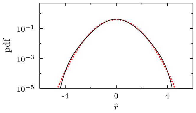
Figure 25: Distribution of the aggregated returns, here denoted by $\widetilde{r}$, for fixed covariances from S&P 500 daily data dataset, $\Delta t$ = 1 trading day and 25 data points per interval. The circles show a normal distribution. Taken from Ref. [54].

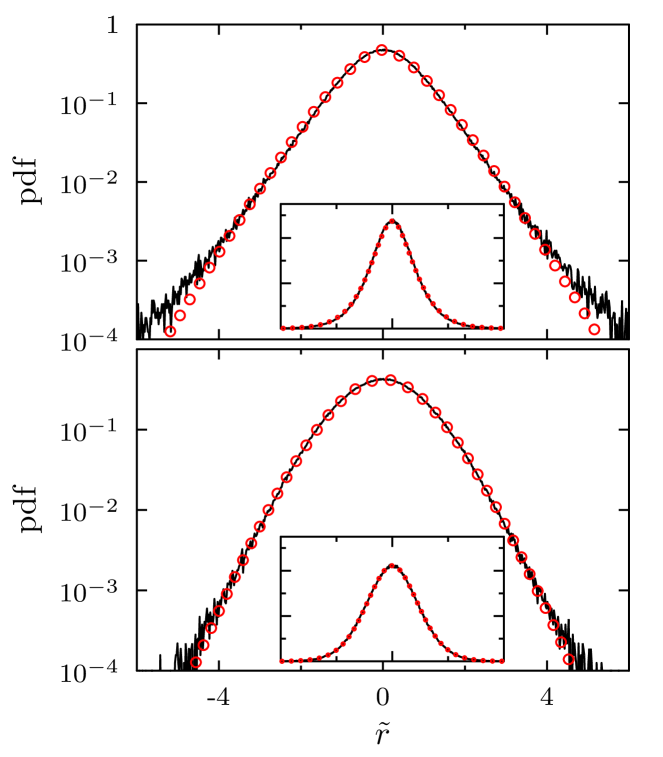
Figure 26: Empirical distributions of the aggregated returns (black) for $\Delta t=1$ (top) and $\Delta t=20$ (bottom) from S&P 500 daily data dataset. Model distribution $\langle p\rangle_{\mathrm{GG}}^{(\mathrm{aggr})}(\widetilde{r})$ is indicated by red circles. Taken from Ref. [54].

5 Conclusions

We empirically analyzed multivariate return distributions of the US stock markets in the year 2014. Strong correlations are present which fluctuate in time because the company performances, the business relations and the traders’ market expectations change. To assess this non–stationarity and to quantitatively describe the multivariate distributions, we apply a random matrix model recently put forward and presented with formulae for the data analyses in I.

We carry out the empirical analysis on (short) epochs and long intervals. To this end, we rotate the data into the eigenbasis of the correlation matrix. As opposed to the univariate distributions of the original, unrotated returns, the univariate distributions of the rotated returns depend on the eigenvalues of the correlation matrix and thus contain the full information on the correlated system. To accumulate statistics we also resort to aggregation.

We find heavy tails which are very well described by an algebraic distributions on the epochs and the Algebraic–Algebraic model on the long interval. Thus, the distributions on the epochs are characterized by only one fit parameter. Having that fixed, the distributions on the long interval depend on just two fit parameters which can readily be determined.

Importantly, the distributions on the epochs on the one hand and on the long interval on the other hand differ in the empirical analysis and their functional forms of the model are different. The tails on the long interval become heavier. Moreover, comparing two long intervals demonstrates that the fluctuations of the correlation further accumulated. This clearly confirms the model of I. The non–stationary fluctuations of the correlations lift the tails.

Appendix A Ticker Symbols

A.1 List of ticker symbols for intraday data set from NYSE

A, AA, AAPL, ABBV, ABC, ABT, ACE, ACN, ACT, ADBE, ADI, ADM, ADP, ADS, ADSK, ADT, AEE, AEP, AES, AET, AFL, AGN, AIG, AIV, AIZ, AKAM, ALL, ALLE, ALTR, ALXN, AMAT, AME, AMGN, AMP, AMT, AMZN, AN, AON, APA, APC, APD, APH, ARG, ATI, AVB, AVP, AVY, AXP, AZO, BA, BAC, BAX, BBBY, BBT, BBY, BCR, BDX, BEN, BHI, BIIB, BK, BLK, BLL, BMY, BRCM, BSX, BWA, BXP, C, CA, CAG, CAH, CAM, CAT, CB, CBG, CBS, CCE, CCI, CCL, CELG, CERN, CF, CFN, CHK, CHRW, CI, CINF, CL, CLX, CMA, CMCSA, CME, CMG, CMI, CMS, CNP, CNX, COF, COG, COH, COL, COP, COST, COV, CPB, CRM, CSC, CSCO, CSX, CTAS, CTL, CTSH, CTXS, CVC, CVS, CVX, D, DAL, DD, DE, DFS, DG, DGX, DHI, DHR, DIS, DISCA, DLPH, DLTR, DNB, DNR, DO, DOV, DOW, DPS, DRI, DTE, DTV, DUK, DVA, DVN, EA, EBAY, ECL, ED, EFX, EIX, EL, EMC, EMN, EMR, EOG, EQR, EQT, ESRX, ESV, ETFC, ETN, ETR, EW, EXC, EXPD, EXPE, F, FAST, FB, FCX, FDO, FDX, FE, FFIV, FIS, FISV, FITB, FLIR, FLR, FLS, FMC, FOSL, FOXA, FSLR, FTI, FTR, GAS, GCI, GD, GE, GGP, GILD, GIS, GLW, GM, GME, GNW, GOOG, GPC, GPS, GRMN, GS, GT, GWW, HAL, HAR, HAS, HBAN, HCBK, HCN, HCP, HD, HES, HIG, HOG, HON, HOT, HP, HPQ, HRB, HRL, HRS, HSP, HST, HSY, HUM, IBM, ICE, IFF, INTC, INTU, IP, IPG, IR, IRM, ISRG, ITW, IVZ, JCI, JEC, JNJ, JNPR, JOY, JPM, JWN, K, KEY, KIM, KLAC, KMB, KMI, KMX, KO, KR, KRFT, KSS, KSU, L, LB, LEG, LEN, LH, LIFE, LLL, LLTC, LLY, LM, LMT, LNC, LO, LOW, LRCX, LUK, LUV, LYB, M, MA, MAC, MAR, MAS, MAT, MCD, MCHP, MCK, MCO, MDLZ, MDT, MET, MHFI, MHK, MJN, MKC, MMC, MMM, MNST, MO, MON, MOS, MPC, MRK, MRO, MS, MSFT, MSI, MTB, MU, MUR, MWV, MYL, NBR, NDAQ, NE, NEE, NEM, NFLX, NFX, NI, NKE, NLSN, NOC, NOV, NRG, NSC, NTAP, NTRS, NUE, NVDA, NWL, NWSA, OI, OKE, OMC, ORCL, ORLY, OXY, PAYX, PBCT, PBI, PCAR, PCG, PCL, PCLN, PCP, PDCO, PEG, PEP, PETM, PFE, PFG, PG, PGR, PH, PHM, PKI, PLD, PLL, PM, PNC, PNR, PNW, POM, PPG, PPL, PRGO, PRU, PSA, PSX, PVH, PWR, PX, PXD, QCOM, QEP, R, RAI, RDC, REGN, RF, RHI, RHT, RIG, RL, ROK, ROP, ROST, RRC, RSG, RTN, SBUX, SCG, SCHW, SE, SEE, SHW, SIAL, SJM, SLB, SNA, SNDK, SNI, SO, SPG, SPLS, SRCL, SRE, STI, STJ, STT, STX, STZ, SWK, SWN, SWY, SYK, SYMC, SYY, T, TAP, TDC, TE, TEG, TEL, TGT, THC, TIF, TJX, TMK, TMO, TRIP, TROW, TRV, TSN, TSO, TSS, TWC, TWX, TXN, TXT, TYC, UNH, UNM, UNP, UPS, URBN, USB, UTX, V, VAR, VFC, VIAB, VLO, VMC, VNO, VRSN, VRTX, VTR, VZ, WAG, WAT, WDC, WEC, WFC, WFM, WHR, WIN, WM, WMB, WMT, WU, WY, WYN, WYNN, XEL, XL, XLNX, XOM, XRAY, XRX, XYL, YHOO, YUM

A.2 List of ticker symbols for daily data set from Yahoo! Finance

AA, AAPL, ABT, ADBE, ADI, ADM, ADP, ADSK, AEP, AES, AET, AFL, AGN, AIG, ALTR, AMAT, AMD, AMGN, AON, APA, APC, APD, APH, ARG, AVP, AVY, AXP, AZO, BA, BAC, BAX, BBT, BBY, BCR, BDX, BEN, BF.B, BHI, BIG, BIIB, BK, BLL, BMC, BMS, BMY, C, CA, CAG, CAH, CAT, CB, CCE, CCL, CELG, CERN, CI, CINF, CL, CLF, CLX, CMA, CMCSA, CMI, CMS, CNP, COG, COP, COST, CPB, CSC, CSCO, CSX, CTAS, CTL, CVH, CVS, CVX, D, DD, DE, DELL, DHR, DIS, DNB, DOV, DOW, DTE, DUK, ECL, ED, EFX, EIX, EMC, EMR, EOG, EQT, ETN, ETR, EXC, F, FAST, FDO, FDX, FHN, FISV, FITB, FLS, FMC, FRX, GAS, GCI, GD, GE, GIS, GLW, GPC, GPS, GT, GWW, HAL, HAS, HBAN, HCP, HD, HES, HNZ, HOG, HON, HOT, HP, HPQ, HRB, HRL, HRS, HST, HSY, HUM, IBM, IFF, IGT, INTC, IP, IPG, IR, ITW, JCI, JCP, JEC, JNJ, JPM, JWN, K, KEY, KIM, KLAC, KMB, KO, KR, L, LEG, LEN, LH, LLTC, LLY, LM, LMT, LNC, LOW, LSI, LTD, LUK, LUV, MAS, MAT, MCD, MDT, MHP, MKC, MMC, MMM, MO, MOLX, MRK, MRO, MSFT, MSI, MTB, MU, MUR, MWV, MYL, NBL, NBR, NE, NEE, NEM, NI, NKE, NOC, NSC, NTRS, NU, NUE, NWL, OI, OKE, OMC, ORCL, OXY, PAYX, PBCT, PBI, PCAR, PCG, PCL, PCP, PEP, PFE, PG, PGR, PH, PHM, PLL, PNC, PNW, POM, PPG, PPL, PSA, QCOM, R, RDC, RF, ROK, ROST, RRD, RSH, RTN, S, SCG, SCHW, SEE, SHW, SIAL, SLB, SLM, SNA, SO, SPLS, STI, STJ, STT, SUN, SVU, SWK, SWN, SWY, SYK, SYMC, SYY, T, TAP, TE, TEG, TER, TGT, THC, TIF, TJX, TLAB, TMK, TMO, TROW, TRV, TSN, TSO, TXN, TXT, TYC, UNH, UNP, USB, UTX, VAR, VFC, VLO, VMC, VNO, VZ, WAG, WDC, WEC, WFC, WFM, WHR, WM, WMB, WMT, WPO, WY, X, XEL, XL, XLNX, XOM, XRAY, XRX, ZION

Appendix B Tables for Secs. 2.3, 3.2

B.1 Overview of the start and end of intervals for 25 trading days

Table 1: Overview of the start and end of intervals (month-day) with a length of 25 trading days for 2014.

interval 1	01-02 to 02-06
interval 2	02-07 to 03-14
interval 3	03-17 to 04-21
interval 4	04-22 to 05-27
interval 5	05-28 to 07-01
interval 6	07-02 to 08-06
interval 7	08-07 to 09-11
interval 8	09-12 to 10-16
interval 9	10-17 to 11-20
interval 10	11-21 to 12-29

B.2 Parameters $l_{\mathrm{rot}}$, $\chi^{2}_{\mathrm{ln}}$ and $\chi^{2}_{\mathrm{lin}}$ for fits on the epochs

Table 2: Parameters $l_{\mathrm{rot}}$, $\chi^{2}_{\mathrm{ln}}$ and $\chi^{2}_{\mathrm{lin}}$ determined by logarithmic and linear fit with return horizon $\Delta t$.

date	fit	$\Delta t$	$l_{\mathrm{rot}}$	$\chi^{2}_{\mathrm{ln}}$	$\chi^{2}_{\mathrm{lin}}$
Dec. 8	log	1 s	2.936	0.008	—
Dec. 8	lin	1 s	2.742	—	$1.231\cdot 10^{-6}$
Dec. 17	log	1 s	2.688	0.006	—
Dec. 17	lin	1 s	2.351	—	$1.076\cdot 10^{-5}$
Feb. 20	log	10 s	3.217	0.017	—
Feb. 20	lin	10 s	3.108	—	$8.662\cdot 10^{-6}$
Jun. 02	log	10 s	3.249	0.015	—
Jun. 02	lin	10 s	3.008	—	$1.181\cdot 10^{-5}$

B.3 Averaged parameters $\langle l_{\mathrm{rot}}\rangle$, $\langle\chi^{2}_{\mathrm{ln}}\rangle$ and $\langle\chi^{2}_{\mathrm{lin}}\rangle$ for fits on the epochs

Table 3: Averaged parameters $\langle l_{\mathrm{rot}}\rangle$, $\langle\chi^{2}_{\mathrm{ln}}\rangle$ and $\langle\chi^{2}_{\mathrm{lin}}\rangle$ determined by logarithmic and linear fit with return horizon $\Delta t$.

fit	$\Delta t$	$\langle l\rangle_{\mathrm{rot}}$	$\langle\chi^{2}_{\mathrm{ln}}\rangle$	$\langle\chi^{2}_{\mathrm{lin}}\rangle$
log	1 s	2.602	0.025	—
lin	1 s	2.295	—	$8.781\cdot 10^{-6}$
log	10 s	3.531	0.053	—
log	10 s	3.717	—	$5.136\cdot 10^{-6}$

B.4 Fitting parameters for fits on the long interval

Table 4: Fitting parameters for distributions of the aggregated returns on long intervals in trading days (td) and return horizon $\Delta t$ determined by logarithmic and linear fit.

interval	fit	$\Delta t$	interval	$\langle p\rangle_{\mathrm{GG}}$	$\langle p\rangle_{\mathrm{GA}}$	$\langle p\rangle_{\mathrm{GA}}$	$\langle p\rangle_{\mathrm{AG}}$	$\langle p\rangle_{\mathrm{AA}}$	$\langle p\rangle_{\mathrm{AA}}$
number			length	$N$	$L_{\mathrm{rot}}$	$N$	$N$	$L_{\mathrm{rot}}$	$N$
interval  9	log	1 s	25 td	0.794	3.466	2.436	2.848	99.551	2.906
interval  9	lin	1 s	25 td	2.038	4.425	5.078	5.986	100.355	6.149
interval  8	log	10 s	25 td	1.194	5.433	5.202	4.207	11.032	10.031
interval  8	lin	10 s	25 td	2.994	7.435	10.107	5.442	13.562	19.029
interval  1	log	1 s	50 td	0.814	3.548	2.154	3.052	99.606	3.118
interval  1	lin	1 s	50 td	2.032	4.295	4.717	5.959	100.352	6.122
interval  2	log	10 s	50 td	1.210	5.284	4.642	4.343	13.498	6.433
interval  2	lin	10 s	50 td	3.269	9.925	15.026	5.236	13.562	6.651

B.5 Values of $\chi^{2}$ for fits on the long interval

Table 5: Values of $\chi^{2}$ for distributions of the aggregated returns on long intervals in trading days (td) and return horizon $\Delta t$ determined by logarithmic and linear fit.

interval	fit	$\Delta t$	interval	$\langle p\rangle_{\mathrm{GG}}$	$\langle p\rangle_{\mathrm{GA}}$	$\langle p\rangle_{\mathrm{AG}}$	$\langle p\rangle_{\mathrm{AA}}$
length			number	$\chi^{2}_{\mathrm{ln}}$ / $\chi^{2}_{\mathrm{lin}}$
25 td	log	1 s	interval  9	0.060	0.002	0.003	0.003
25 td	lin	1 s	interval  9	$1.552\cdot 10^{-4}$	$5.625\cdot 10^{-7}$	$1.694\cdot 10^{-6}$	$1.809\cdot 10^{-6}$
25 td	log	10 s	interval  8	0.066	0.008	0.008	0.008
25 td	lin	10 s	interval  8	$4.770\cdot 10^{-5}$	$3.272\cdot 10^{-7}$	$5.545\cdot 10^{-6}$	$3.967\cdot 10^{-7}$
50 td	log	1 s	interval  1	0.049	0.003	0.005	0.005
50 td	lin	1 s	interval  1	$1.426\cdot 10^{-4}$	$7.746\cdot 10^{-7}$	$3.241\cdot 10^{-6}$	$3.427\cdot 10^{-6}$
50 td	log	10 s	interval  2	0.058	0.007	0.008	0.007
50 td	lin	10 s	interval  2	$3.852\cdot 10^{-5}$	$1.136\cdot 10^{-7}$	$6.128\cdot 10^{-6}$	$3.899\cdot 10^{-6}$

B.6 Averaged fitting parameters for fits on the long interval

Table 6: Averaged fitting parameters for distributions of the aggregated returns on long intervals in trading days (td) and return horizon $\Delta t$ determined by logarithmic and linear fit.

fit	$\Delta t$	interval	$\langle p\rangle_{\mathrm{GG}}$	$\langle p\rangle_{\mathrm{GA}}$	$\langle p\rangle_{\mathrm{GA}}$	$\langle p\rangle_{\mathrm{AG}}$	$\langle p\rangle_{\mathrm{AA}}$	$\langle p\rangle_{\mathrm{AA}}$
		length	$\langle N\rangle$	$\langle L_{\mathrm{rot}}\rangle$	$\langle N\rangle$	$\langle N\rangle$	$\langle L_{\mathrm{rot}}\rangle$	$\langle N\rangle$
log	1 s	25 td	0.806	3.521	2.163	3.055	85.810	3.190
log	1 s	50 td	0.769	3.355	2.008	2.563	64.598	2.729
lin	1 s	25 td	2.023	4.332	4.831	6.020	90.294	6.241
lin	1 s	50 td	1.892	3.923	4.080	4.735	81.697	5.007
log	10 s	25 td	1.221	5.473	5.023	4.669	19.860	11.196
log	10 s	50 td	1.138	5.169	4.774	3.674	11.260	10.420
lin	10 s	25 td	3.360	18.369	32.026	7.143	15.534	17.773
lin	10 s	50 td	3.158	12.432	20.159	6.184	15.229	17.911

Appendix C Tables of fitting parameters for Sec. 3.3

C.1 Intervals with a length of 25 trading days

Table 7: Fitting parameters for distributions of the aggregated returns for long intervals (25 trading days) with $\Delta t=1\,\mathrm{s}$ determined on a logarithmic scale.

	$\langle p\rangle_{\mathrm{GG}}$	$\langle p\rangle_{\mathrm{GA}}$	$\langle p\rangle_{\mathrm{GA}}$	$\langle p\rangle_{\mathrm{AG}}$	$\langle p\rangle_{\mathrm{AA}}$	$\langle p\rangle_{\mathrm{AA}}$
	$N$	$L_{\mathrm{rot}}$	$N$	$N$	$L_{\mathrm{rot}}$	$N$
interval  1	0.847	3.664	2.285	3.518	99.727	3.604
interval  2	0.841	3.652	2.157	3.391	99.693	3.471
interval  3	0.906	3.980	2.143	4.769	100.056	4.923
interval  4	0.781	3.391	2.086	2.603	99.488	2.651
interval  5	0.733	3.213	2.096	2.217	9.310	2.855
interval  6	0.780	3.407	2.335	2.686	51.624	2.790
interval  7	0.795	3.467	2.207	2.841	99.550	2.899
interval  8	0.741	3.282	1.745	2.171	99.378	2.206
interval  9	0.794	3.466	2.436	2.848	99.551	2.906
interval 10	0.845	3.691	2.140	3.506	99.724	3.592

Table 8: Fitting parameters for distributions of the aggregated returns for long intervals (25 trading days) with $\Delta t=1\,\mathrm{s}$ determined on a linear scale.

	$\langle p\rangle_{\mathrm{GG}}$	$\langle p\rangle_{\mathrm{GA}}$	$\langle p\rangle_{\mathrm{GA}}$	$\langle p\rangle_{\mathrm{AG}}$	$\langle p\rangle_{\mathrm{AA}}$	$\langle p\rangle_{\mathrm{AA}}$
	$N$	$L_{\mathrm{rot}}$	$N$	$N$	$L_{\mathrm{rot}}$	$N$
interval  1	2.128	4.683	5.503	7.268	100.55	7.519
interval  2	2.151	4.807	5.762	7.657	96.610	7.950
interval  3	2.113	4.350	4.550	7.120	100.653	7.361
interval  4	2.029	4.409	5.051	5.921	100.345	6.081
interval  5	2.018	4.519	5.359	5.837	100.322	5.992
interval  6	2.029	4.349	4.884	5.922	100.340	6.082
interval  7	2.009	4.159	4.356	5.747	100.299	5.898
interval  8	1.750	3.607	3.684	3.555	13.566	4.067
interval  9	2.038	4.425	5.078	5.986	100.355	6.149
interval 10	1.962	4.015	4.083	5.191	100.152	5.311

Table 9: Fitting parameters for distributions of the aggregated returns for long intervals (25 trading days) with $\Delta t=10\,\mathrm{s}$ determined on a logarithmic scale.

	$\langle p\rangle_{\mathrm{GG}}$	$\langle p\rangle_{\mathrm{GA}}$	$\langle p\rangle_{\mathrm{GA}}$	$\langle p\rangle_{\mathrm{AG}}$	$\langle p\rangle_{\mathrm{AA}}$	$\langle p\rangle_{\mathrm{AA}}$
	$N$	$L_{\mathrm{rot}}$	$N$	$N$	$L_{\mathrm{rot}}$	$N$
interval  1	1.263	5.294	4.117	4.922	13.292	8.336
interval  2	1.269	5.287	3.988	4.989	89.086	5.199
interval  3	1.436	5.874	4.540	8.179	15.396	14.738
interval  4	1.132	5.044	4.525	3.570	9.599	8.039
interval  5	1.103	4.882	4.267	3.298	9.039	7.719
interval  6	1.153	5.579	5.839	3.806	12.770	16.754
interval  7	1.276	5.641	5.236	5.189	13.169	12.410
interval  8	1.194	5.433	5.202	4.207	11.032	10.031
interval  9	1.125	5.937	6.832	3.577	12.594	16.942
interval 10	1.257	5.756	5.683	4.953	12.626	11.791

Table 10: Fitting parameters for distributions of the aggregated returns for long intervals (25 trading days) with $\Delta t=10\,\mathrm{s}$ determined on a linear scale.

	$\langle p\rangle_{\mathrm{GG}}$	$\langle p\rangle_{\mathrm{GA}}$	$\langle p\rangle_{\mathrm{GA}}$	$\langle p\rangle_{\mathrm{AG}}$	$\langle p\rangle_{\mathrm{AA}}$	$\langle p\rangle_{\mathrm{AA}}$
	$N$	$L_{\mathrm{rot}}$	$N$	$N$	$L_{\mathrm{rot}}$	$N$
interval  1	3.427	16.771	28.897	7.424	16.025	17.623
interval  2	3.523	29.118	53.651	7.976	16.741	17.125
interval  3	3.621	10.421	15.514	8.669	17.183	16.892
interval  4	3.194	11.629	18.703	6.283	14.205	18.755
interval  5	3.272	26.450	48.574	6.638	15.940	17.443
interval  6	3.314	10.871	16.974	6.841	15.716	16.996
interval  7	3.447	12.149	19.418	7.572	15.450	17.827
interval  8	2.994	7.435	10.107	5.442	13.562	19.029
interval  9	3.427	48.002	91.603	7.405	15.272	18.024
interval 10	3.378	10.846	16.814	7.176	15.243	18.014

Table 11: Averaged $\chi^{2}$ for logarithmic and linear scale ($\langle\chi^{2}_{\mathrm{ln}}\rangle$ and $\langle\chi^{2}_{\mathrm{lin}}\rangle$) with $\Delta t=1\,\mathrm{s}$ and $\Delta t=10\,\mathrm{s}$ for the model distributions on the long interval.

	$\Delta t=1\,\mathrm{s}$		$\Delta t=10\,\mathrm{s}$
	$\langle\chi^{2}_{\mathrm{ln}}\rangle$	$\langle\chi^{2}_{\mathrm{lin}}\rangle$	$\langle\chi^{2}_{\mathrm{ln}}\rangle$	$\langle\chi^{2}_{\mathrm{lin}}\rangle$
GG	0.051	$1.524\cdot 10^{-4}$	0.066	$4.268\cdot 10^{-5}$
GA	0.003	$1.109\cdot 10^{-6}$	0.013	$3.334\cdot 10^{-7}$
AG	0.006	$3.488\cdot 10^{-6}$	0.014	$5.668\cdot 10^{-6}$
AA	0.006	$3.562\cdot 10^{-6}$	0.014	$3.247\cdot 10^{-6}$

C.2 Intervals with a length of 50 trading days

Table 12: Fitting parameters for distributions of the aggregated returns for long intervals (50 trading days) with $\Delta t=1\,\mathrm{s}$ determined on a logarithmic scale.

	$\langle p\rangle_{\mathrm{GG}}$	$\langle p\rangle_{\mathrm{GA}}$	$\langle p\rangle_{\mathrm{GA}}$	$\langle p\rangle_{\mathrm{AG}}$	$\langle p\rangle_{\mathrm{AA}}$	$\langle p\rangle_{\mathrm{AA}}$
	$N$	$L_{\mathrm{rot}}$	$N$	$N$	$L_{\mathrm{rot}}$	$N$
interval  1	0.814	3.548	2.154	3.052	99.606	3.118
interval  2	0.820	3.576	2.050	3.062	99.608	3.129
interval  3	0.736	3.210	2.063	2.205	12.281	2.608
interval  4	0.677	2.978	1.606	1.683	11.952	1.920
interval  5	0.799	3.463	2.167	2.813	99.544	2.870

Table 13: Fitting parameters for distributions of the aggregated returns for long intervals (50 trading days) with $\Delta t=1\,\mathrm{s}$ determined on a linear scale.

	$\langle p\rangle_{\mathrm{GG}}$	$\langle p\rangle_{\mathrm{GA}}$	$\langle p\rangle_{\mathrm{GA}}$	$\langle p\rangle_{\mathrm{AG}}$	$\langle p\rangle_{\mathrm{AA}}$	$\langle p\rangle_{\mathrm{AA}}$
	$N$	$L_{\mathrm{rot}}$	$N$	$N$	$L_{\mathrm{rot}}$	$N$
interval  1	2.032	4.295	4.717	5.959	100.352	6.122
interval  2	1.960	3.997	3.989	5.236	100.165	5.359
interval  3	1.902	3.972	4.190	4.706	100.026	4.802
interval  4	1.662	3.435	3.490	3.098	7.925	3.982
interval  5	1.905	3.917	4.014	4.677	100.019	4.77

Table 14: Fitting parameters for distributions of the aggregated returns for long intervals (50 trading days) with $\Delta t=10\,\mathrm{s}$ determined on a logarithmic scale.

	$\langle p\rangle_{\mathrm{GG}}$	$\langle p\rangle_{\mathrm{GA}}$	$\langle p\rangle_{\mathrm{GA}}$	$\langle p\rangle_{\mathrm{AG}}$	$\langle p\rangle_{\mathrm{AA}}$	$\langle p\rangle_{\mathrm{AA}}$
	$N$	$L_{\mathrm{rot}}$	$N$	$N$	$L_{\mathrm{rot}}$	$N$
interval  1	1.204	5.075	3.886	4.227	11.145	8.179
interval  2	1.210	5.284	4.642	4.343	13.498	6.433
interval  3	1.067	4.981	4.821	3.070	10.748	13.888
interval  4	1.078	4.844	4.349	3.139	8.651	7.481
interval  5	1.129	5.660	6.170	3.590	12.259	16.119

Table 15: Fitting parameters for distributions of the aggregated returns for long intervals (50 trading days) with $\Delta t=10\,\mathrm{s}$ determined on a linear scale.

	$\langle p\rangle_{\mathrm{GG}}$	$\langle p\rangle_{\mathrm{GA}}$	$\langle p\rangle_{\mathrm{GA}}$	$\langle p\rangle_{\mathrm{AG}}$	$\langle p\rangle_{\mathrm{AA}}$	$\langle p\rangle_{\mathrm{AA}}$
	$N$	$L_{\mathrm{rot}}$	$N$	$N$	$L_{\mathrm{rot}}$	$N$
interval  1	3.331	17.148	29.778	6.924	15.983	17.524
interval  2	3.269	9.925	15.027	6.651	14.588	18.579
interval  3	3.127	12.721	21.0377	5.987	16.685	16.930
interval  4	2.791	7.306	10.212	4.718	12.886	18.958
interval  5	3.274	15.061	25.620	6.639	16.001	17.563

Table 16: Averaged $\chi^{2}$ for logarithmic and linear scale ($\langle\chi^{2}_{\mathrm{ln}}\rangle$ and $\langle\chi^{2}_{\mathrm{lin}}\rangle$) with $\Delta t=1\,\mathrm{s}$ and $\Delta t=10\,\mathrm{s}$ for the model distributions on the long interval.

	$\Delta t=1\,\mathrm{s}$		$\Delta t=10\,\mathrm{s}$
	$\langle\chi^{2}_{\mathrm{ln}}\rangle$	$\langle\chi^{2}_{\mathrm{lin}}\rangle$	$\langle\chi^{2}_{\mathrm{ln}}\rangle$	$\langle\chi^{2}_{\mathrm{lin}}\rangle$
GG	0.052	$1.805\cdot 10^{-4}$	0.063	$5.066\cdot 10^{-5}$
GA	0.003	$1.323\cdot 10^{-6}$	0.007	$2.759\cdot 10^{-7}$
AG	0.004	$4.022\cdot 10^{-6}$	0.008	$7.624\cdot 10^{-6}$
AA	0.004	$3.396\cdot 10^{-6}$	0.007	$7.994\cdot 10^{-6}$

References

- [1] Rosario N. Mantegna and H. Eugene Stanley “Introduction to Econophysics: Correlations and Complexity in Finance” Cambridge: Cambridge University Press, 1999
- [2] Ryszard Kutner et al. “Econophysics and sociophysics: Their milestones challenges” In Physica A: Statistical Mechanics and its Applications 516, 2019, pp. 240 –253 DOI: https://doi.org/10.1016/j.physa.2018.10.019
- [3] Benoit Mandelbrot “The Variation of Certain Speculative Prices” In The Journal of Business 36.4 University of Chicago Press, 1963, pp. 394–419 URL: http://www.jstor.org/stable/2350970
- [4] Parameswaran Gopikrishnan, Martin Meyer, Luís A. Nunes N. Amaral and H. Eugene Stanley “Inverse cubic law for the distribution of stock price variations” In The European Physical Journal B - Condensed Matter and Complex Systems 3.2, 1998, pp. 139–140 DOI: 10.1007/s100510050292
- [5] Vasiliki Plerou et al. “Scaling of the distribution of price fluctuations of individual companies” In Phys. Rev. E 60 American Physical Society, 1999, pp. 6519–6529 DOI: 10.1103/PhysRevE.60.6519
- [6] Jean-Philippe Bouchaud, Yuval Gefen, Marc Potters and Matthieu Wyart “Fluctuations and response in financial markets: the subtle nature of ‘random’ price changes” In Quantitative Finance 4.2 Informa UK Limited, 2004, pp. 176–190 DOI: 10.1080/14697680400000022
- [7] J. Doyne Farmer et al. “What really causes large price changes?” In Quantitative Finance 4.4 Routledge, 2004, pp. 383–397 DOI: 10.1080/14697680400008627
- [8] Jean-Philippe Bouchaud, J. Doyne Farmer and Fabrizio Lillo “CHAPTER 2 - How Markets Slowly Digest Changes in Supply and Demand” In Handbook of Financial Markets: Dynamics and Evolution, Handbooks in Finance San Diego: North-Holland, 2009, pp. 57–160 DOI: https://doi.org/10.1016/B978-012374258-2.50006-3
- [9] Laurent Laloux, Pierre Cizeau, Jean-Philippe Bouchaud and Marc Potters “Noise Dressing of Financial Correlation Matrices” In Phys. Rev. Lett. 83 American Physical Society, 1999, pp. 1467–1470 DOI: 10.1103/PhysRevLett.83.1467
- [10] Parameswaran Gopikrishnan, Bernd Rosenow, Vasiliki Plerou and H. Eugene Stanley “Quantifying and interpreting collective behavior in financial markets” In Phys. Rev. E 64 American Physical Society, 2001, pp. 035106(R) DOI: 10.1103/PhysRevE.64.035106
- [11] Vasiliki Plerou et al. “Random matrix approach to cross correlations in financial data” In Phys. Rev. E 65 American Physical Society, 2002, pp. 066126 DOI: 10.1103/PhysRevE.65.066126
- [12] Robert Engle “Dynamic Conditional Correlation” In Journal of Business & Economic Statistics 20.3 Taylor & Francis, 2002, pp. 339–350 DOI: 10.1198/073500102288618487
- [13] Yiu Kuen Tse and Albert K. C. Tsui “A Multivariate Generalized Autoregressive Conditional Heteroscedasticity Model With Time-Varying Correlations” In Journal of Business & Economic Statistics 20.3 Taylor & Francis, 2002, pp. 351–362 DOI: 10.1198/073500102288618496
- [14] Cathrin Van Emmerich “Modelling correlation as a stochastic process” In Preprint, 2006 URL: https://www.imacm.uni-wuppertal.de/fileadmin/imacm/preprints/amna_06_03.pdf
- [15] Jun Ma “Pricing Foreign Equity Options with Stochastic Correlation and Volatility.” In Annals of Economics & Finance 10.2, 2009, pp. 303–327
- [16] Vasyl Golosnoy, Bastian Gribisch and Roman Liesenfeld “The conditional autoregressive Wishart model for multivariate stock market volatility” In Journal of Econometrics 167.1, 2012, pp. 211–223 DOI: https://doi.org/10.1016/j.jeconom.2011.11.004
- [17] Gian Piero Aielli “Dynamic Conditional Correlation: On Properties and Estimation” In Journal of Business & Economic Statistics 31.3 Taylor & Francis, 2013, pp. 282–299 DOI: 10.1080/07350015.2013.771027
- [18] Long Teng, Matthias Ehrhardt and Michael Günther “Modelling stochastic correlation” In Journal of Mathematics in Industry 6.1, 2016, pp. 2 DOI: 10.1186/s13362-016-0018-4
- [19] Luc Bauwens, Manuela Braione and Giuseppe Storti “Multiplicative conditional correlation models for realized covariance matrices” CORE Discussion Paper - 2016/41, 2016 URL: http://hdl.handle.net/2078.1/178422
- [20] Alan G. Hawkes “Hawkes processes and their applications to finance: a review” In Quantitative Finance 18.2 Routledge, 2018, pp. 193–198 DOI: 10.1080/14697688.2017.1403131
- [21] Christian M. Hafner, Helmut Herwartz and Simone Maxand “Identification of structural multivariate GARCH models” Annals Issue: Time Series Analysis of Higher Moments and Distributions of Financial Data In Journal of Econometrics 227.1, 2022, pp. 212–227 DOI: https://doi.org/10.1016/j.jeconom.2020.07.019
- [22] Michael C. Münnix et al. “Identifying States of a Financial Market” In Scientific Reports 2, 2012, pp. 644 DOI: 10.1038/srep00644
- [23] Shanshan Wang, Sebastian Gartzke, Michael Schreckenberg and Thomas Guhr “Quasi-stationary states in temporal correlations for traffic systems: Cologne orbital motorway as an example” In Journal of Statistical Mechanics: Theory and Experiment 2020.10 IOP Publishing, 2020, pp. 103404 DOI: 10.1088/1742-5468/abbcd3
- [24] Shanshan Wang, Sebastian Gartzke, Michael Schreckenberg and Thomas Guhr “Collective behavior in the North Rhine-Westphalia motorway network” In Journal of Statistical Mechanics: Theory and Experiment 2021.12 IOP Publishing, 2021, pp. 123401 DOI: 10.1088/1742-5468/ac3662
- [25] Henrik M. Bette, Edgar Jungblut and Thomas Guhr “Nonstationarity in correlation matrices for wind turbine SCADA-data” In Wind Energy 26.8, 2023, pp. 826–849 DOI: https://doi.org/10.1002/we.2843
- [26] G. William Schwert “Why does stock market volatility change over time?” In The journal of finance 44.5 Wiley Online Library, 1989, pp. 1115–1153 DOI: 10.1111/j.1540-6261.1989.tb02647.x
- [27] Benoit B. Mandelbrot “”The variation of certain speculative prices”” In Fractals and Scaling in Finance: Discontinuity, Concentration, Risk. Selecta Volume E New York, NY: Springer New York, 1997, pp. 371–418 DOI: 10.1007/978-1-4757-2763-0˙14
- [28] Geert Bekaert and Guojun Wu “Asymmetric Volatility and Risk in Equity Markets” In The Review of Financial Studies 13.1, 2000, pp. 1–42 DOI: 10.1093/rfs/13.1.1
- [29] Geert Bekaert and Marie Hoerova “The VIX, the variance premium and stock market volatility” Analysis of Financial Data In Journal of Econometrics 183.2, 2014, pp. 181–192 DOI: https://doi.org/10.1016/j.jeconom.2014.05.008
- [30] Mieszko Mazur, Man Dang and Miguel Vega “COVID-19 and the march 2020 stock market crash. Evidence from S&P1500” In Finance Research Letters 38, 2021, pp. 101690 DOI: https://doi.org/10.1016/j.frl.2020.101690
- [31] Karl Pearson “X. On the criterion that a given system of deviations from the probable in the case of a correlated system of variables is such that it can be reasonably supposed to have arisen from random sampling ” In The London, Edinburgh, and Dublin Philosophical Magazine and Journal of Science 50.302 Taylor & Francis, 1900, pp. 157–175 DOI: 10.1080/14786440009463897
- [32] Abe Sklar “Fonctions de répartition à n dimensions et leurs marges” In Publ. Inst. Statist. Univ. Paris 8, 1959, pp. 229–231
- [33] Abe Sklar “Random variables, joint distribution functions, and copulas” In Kybernetika 9.6 Institute of Information TheoryAutomation AS CR, 1973, pp. 449–460
- [34] Roger B. Nelsen “An introduction to copulas” New York: Springer, 2010
- [35] Michael C. Münnix and Rudi Schäfer “A copula approach on the dynamics of statistical dependencies in the US stock market” In Physica A: Statistical Mechanics and its Applications 390.23, 2011, pp. 4251–4259 DOI: https://doi.org/10.1016/j.physa.2011.06.032
- [36] David Salinas et al. “High-dimensional multivariate forecasting with low-rank gaussian copula processes” In Advances in neural information processing systems 32, 2019
- [37] Desislava Chetalova, Rudi Schäfer and Thomas Guhr “Zooming into market states” In Journal of Statistical Mechanics: Theory and Experiment 2015.1 IOP Publishing, 2015, pp. P01029 DOI: 10.1088/1742-5468/2015/01/p01029
- [38] Desislava Chetalova, Marcel Wollschläger and Rudi Schäfer “Dependence structure of market states” In Journal of Statistical Mechanics: Theory and Experiment 2015.8 IOP Publishing, 2015, pp. P08012 DOI: 10.1088/1742-5468/2015/08/p08012
- [39] Yuriy Stepanov, Erik Wellner and Tarek Abou-Zeid “Multi-Asset Correlation Dynamics with Application to Trading” A PhD Project, 2015 DOI: 10.13140/RG.2.2.18674.56009
- [40] Yuriy Stepanov et al. “Stability and hierarchy of quasi-stationary states: financial markets as an example” In Journal of Statistical Mechanics: Theory and Experiment 2015.8 IOP Publishing, 2015, pp. P08011 DOI: 10.1088/1742-5468/2015/08/p08011
- [41] Philip Rinn et al. “Dynamics of quasi-stationary systems: Finance as an example” In EPL (Europhysics Letters) 110.6 IOP Publishing, 2015, pp. 68003 DOI: 10.1209/0295-5075/110/68003
- [42] Hirdesh K. Pharasi et al. “Identifying long-term precursors of financial market crashes using correlation patterns” In New Journal of Physics 20.10 IOP Publishing, 2018, pp. 103041 DOI: 10.1088/1367-2630/aae7e0
- [43] Anton J. Heckens, Sebastian M. Krause and Thomas Guhr “Uncovering the Dynamics of Correlation Structures Relative to the Collective Market Motion” In Journal of Statistical Mechanics: Theory and Experiment 2020.10 IOP Publishing, 2020, pp. 103402 DOI: 10.1088/1742-5468/abb6e2
- [44] Anton J. Heckens and Thomas Guhr “A new attempt to identify long-term precursors for endogenous financial crises in the market correlation structures” In Journal of Statistical Mechanics: Theory and Experiment 2022.4 IOP Publishing, 2022, pp. 043401 DOI: 10.1088/1742-5468/ac59ab
- [45] Anton J. Heckens and Thomas Guhr “New collectivity measures for financial covariances and correlations” In Physica A: Statistical Mechanics and its Applications 604, 2022, pp. 127704 DOI: https://doi.org/10.1016/j.physa.2022.127704
- [46] Gautier Marti, Frank Nielsen, Mikołaj Bińkowski and Philippe Donnat “A Review of Two Decades of Correlations, Hierarchies, Networks and Clustering in Financial Markets” In Progress in Information Geometry: Theory and Applications Cham: Springer International Publishing, 2021, pp. 245–274 DOI: 10.1007/978-3-030-65459-7˙10
- [47] Hirdesh K. Pharasi, Eduard Seligman and Thomas H. Seligman “Market states: A new understanding” arXiv:2003.07058, 2020 arXiv:2003.07058 [q-fin.CP]
- [48] Hirdesh K. Pharasi et al. “Dynamics of the market states in the space of correlation matrices with applications to financial markets” arXiv:2107.05663, 2021 arXiv:2107.05663 [q-fin.ST]
- [49] Nick James, Max Menzies and Georg A. Gottwald “On financial market correlation structures and diversification benefits across and within equity sectors” In Physica A: Statistical Mechanics and its Applications 604, 2022, pp. 127682 DOI: https://doi.org/10.1016/j.physa.2022.127682
- [50] Tobias Wand, Martin Heßler and Oliver Kamps “Identifying dominant industrial sectors in market states of the S&P 500 financial data” In Journal of Statistical Mechanics: Theory and Experiment 2023.4 IOP Publishing, 2023, pp. 043402 DOI: 10.1088/1742-5468/accce0
- [51] Martin Heßler, Tobias Wand and Oliver Kamps “Efficient Multi-Change Point Analysis to Decode Economic Crisis Information from the S&P500 Mean Market Correlation” In Entropy 25.9, 2023 DOI: 10.3390/e25091265
- [52] Tobias Wand, Martin Heßler and Oliver Kamps “Memory Effects, Multiple Time Scales and Local Stability in Langevin Models of the S&P500 Market Correlation” In Entropy 25.9, 2023 DOI: 10.3390/e25091257
- [53] Anton J. Heckens, Efstratios Manolakis and Thomas Guhr “Multivariate Distributions in Non–Stationary Complex Systems I: Random Matrix Model and Formulae for Data Analysis” submitted for publication (2024).
- [54] Thilo A. Schmitt, Desislava Chetalova, Rudi Schäfer and Thomas Guhr “Non-stationarity in financial time series: Generic features and tail behavior” In EPL (Europhysics Letters) 103.5 IOP Publishing, 2013, pp. 58003 DOI: 10.1209/0295-5075/103/58003
- [55] Thilo A. Schmitt, Desislava Chetalova, Rudi Schäfer and Thomas Guhr “Credit risk and the instability of the financial system: An ensemble approach” In Europhysics Letters 105.3 EDP Sciences, IOP PublishingSocietà Italiana di Fisica, 2014, pp. 38004 DOI: 10.1209/0295-5075/105/38004
- [56] Thilo Schmitt, Rudi Schäfer and Thomas Guhr “Credit Risk: Taking Fluctuating Asset Correlations into Account” In Journal of Credit Risk 11.3, 2015 DOI: http://doi.org/10.21314/JCR.2015.196
- [57] Desislava Chetalova, Thilo A. Schmitt, Rudi Schäfer and Thomas Guhr “Portfolio return distributions: sample statistics with stochastic correlations” In International Journal of Theoretical and Applied Finance 18.02, 2015, pp. 1550012 DOI: 10.1142/S0219024915500120
- [58] Frederik Meudt, Martin Theissen, Rudi Schäfer and Thomas Guhr “Constructing analytically tractable ensembles of stochastic covariances with an application to financial data” In Journal of Statistical Mechanics: Theory and Experiment 2015.11 IOP PublishingSISSA, 2015, pp. P11025 DOI: 10.1088/1742-5468/2015/11/P11025
- [59] Joachim Sicking, Thomas Guhr and Rudi Schäfer “Concurrent credit portfolio losses” In PLOS ONE 13.2 Public Library of Science, 2018, pp. 1–20 DOI: 10.1371/journal.pone.0190263
- [60] Andreas Mühlbacher and Thomas Guhr “Extreme Portfolio Loss Correlations in Credit Risk” In Risks 6.3, 2018 DOI: 10.3390/risks6030072
- [61] Thomas Guhr and Andreas Schell “Exact multivariate amplitude distributions for non-stationary Gaussian or algebraic fluctuations of covariances or correlations” In Journal of Physics A: Mathematical and Theoretical 54.12 IOP Publishing, 2021, pp. 125002 DOI: 10.1088/1751-8121/abe3c8
- [62] New York stock exchange “Daily TAQ (Trade and Quote)”, https://www.nyse.com/market-data/academics, 2014
- [63] MSCI, S&P Dow Jones Indices LLC and its affiliates “Global Industry Classification Sector (GICS)” MSCI, 2023
- [64] Shanshan Wang, Rudi Schäfer and Thomas Guhr “Average cross-responses in correlated financial markets” In The European Physical Journal B 89.9, 2016, pp. 207 DOI: 10.1140/epjb/e2016-70137-0
- [65] Yahoo! Finance (2013) “Standard & Poor’s 500 stock data)”, http://finance.yahoo.com, 2014
- [66] “Reprint of: Mahalanobis, P.C. (1936) ”On the Generalised Distance in Statistics.”” In Sankhya A 80, 2018, pp. 1–7 URL: https://api.semanticscholar.org/CorpusID:239595337
- [67] Michael C. Münnix, Rudi Schäfer and Thomas Guhr “Impact of the tick-size on financial returns and correlations” In Physica A: Statistical Mechanics and its Applications 389.21, 2010, pp. 4828–4843 DOI: https://doi.org/10.1016/j.physa.2010.06.037
- [68] Vladimir Alexandrovich Marchenko and Leonid Andreevich Pastur “Distribution of eigenvalues for some sets of random matrices” In Matematicheskii Sbornik 114.4 Russian Academy of Sciences, Steklov Mathematical Institute of Russian …, 1967, pp. 507–536 DOI: https://doi.org/10.1070/SM1967v001n04ABEH001994
- [69] Philip R. Bevington and D. Keith Robinson “Data reduction and error analysis for the physical sciences” New York, United States: McGraw-Hill, 2003
- [70] Parameswaran Gopikrishnan et al. “Scaling of the distribution of fluctuations of financial market indices” In Phys. Rev. E 60 American Physical Society, 1999, pp. 5305–5316 DOI: 10.1103/PhysRevE.60.5305
- [71] Xavier Gabaix, Parameswaran Gopikrishnan, Vasiliki Plerou and H. Eugene Stanley “A theory of power-law distributions in financial market fluctuations” In Nature 423.6937, 2003, pp. 267–270 DOI: 10.1038/nature01624
- [72] Juan C. Henao-Londono, Anton J. Heckens and Thomas Guhr “Exact multivariate amplitude distributions in correlated financial markets” https://github.com/juanhenao21/exact_distributions_financial, 2021