Multivariate Distributions in Non–Stationary Complex Systems I: Random Matrix Model and Formulae for Data Analysis

Abstract

Risk assessment for rare events is essential for understanding systemic stability in complex systems. As rare events are typically highly correlated, it is important to study heavy–tailed multivariate distributions of the relevant variables, i.e. their joint probability density functions. Only for few systems, such investigation have been performed. Statistical models are desirable that describe heavy–tailed multivariate distributions, in particular when non–stationarity is present as is typically the case in complex systems. Recently, we put forward such a model based on a separation of time scales. By utilizing random matrices, we showed that the fluctuations of the correlations lift the tails. Here, we present formulae and methods to carry out a data comparisons for complex systems. There are only few fit parameters. Compared to our previous results, we manage to remove in the algebraic cases one out of the two, respectively three, fit parameters which considerably facilitates applications. Furthermore, we explicitly work out the moments of our model distributions. In a forthcoming paper we will apply our model to financial markets.

1 Introduction

Ever more high–quality data accumulated in complex systems of all kinds become available and trigger the need for a better understanding and a quantitative modeling [1, 2]. The data are typically highly correlated, implying that a univariate data analysis is insufficient. Rare events in the often heavy tails of the distributions are especially sensitive for the systemic risk and the stability of a system. Another important aspect of complex systems is their non–stationarity [3, 4, 5, 6, 7]. Finance is a good example, but certainly not the only one. The standard deviations or volatilities which are important statistical estimators fluctuate seemingly erratically over time [8, 9, 10, 11, 12]. The mutual dependencies such as Pearson correlations or copulas [13, 14, 15, 16, 17, 18] which measure the relations within the financial markets show non–stationarity variations as well which plays a particularly important role in states of crisis [4, 19, 20, 21, 22, 23, 24, 25, 26, 27, 28, 29, 30, 31, 32, 33, 34].

Our goal is, for complex systems in general, to assess and quantify non–stationarity and to provide analytical model descriptions for the multivariate distributions. In Refs. [35, 36, 37, 38, 39, 40, 41] we developed a model for the multivariate distributions in the context of credit risk and portfolio optimization. We recently considerably extended it [42] to also properly capture algebraic tails. Here, we present these results in a form directly applicable to data. The model is based on a separation of time scales, guided by the observation that the effects due to non–stationarity accumulate as the length of the considered time intervals increases. We assume a certain behavior, for example approximate stationarity, within short epochs and fluctuating correlations from epoch to epoch. Modeling the latter with random matrices [43, 44, 45, 46], we are able to provide analytical formulae with few parameters for the multivariate distributions in the presence of non–stationarity. Importantly, compared to our formulae in Ref. [42], we manage to reduce the number of fit parameters in the algebraic cases from two to one or three to two, respectively, which is highly useful for applications. We also provide new results on moments. From a formal mathematical point of view, our random–matrix model is a matrix–valued extension of compounding [47] or mixture [48] approaches in statistics, but in contrast to these results, we are on phenomenologically solid grounds. We model a truly existing ensemble of empirical correlation matrices by an ensemble of random matrices. Among many other things, our random–matrix model also gives a justification and interpretation of single–variate ad–hoc approaches [47, 49, 50, 51, 52, 53]. In a forthcoming paper [54] henceforth referred to as II, we will present a careful comparison of financial data analysis with the analytical model.

The paper is organized as follows. In Sec. 2, we give an overview of our random matrix approach and bring the resulting multivariate distributions in forms directly applicable to data. We also calculate the moments of these four model distributions. We give our conclusions in Sec. 3.

2 Random matrix model for multivariate distributions

In Sec. 2.1, we present the salient features of the random matrix model. The process of rotation and aggregation for the analytical distributions with arbitrary kinds of amplitudes is explained in Sec. 2.2. In Secs. 2.3 and 2.4, we specify two forms of multivariate distributions for the epochs and calculate those on the long interval by employing two forms of random matrix ensembles to model the non–stationarity. We arrive at four ensemble averaged multivariate amplitude distributions, described in Sec. 2.5. We calculate the moments in Sec. 2.6.

2.1 Idea and concept

Non–stationarity is ubiquitous in complex systems. Finance provides good examples. Correlation coefficients between different stocks vary when analyzed in a sliding sample window. There is no reason for them to be constant, as the business relations, the company performances, the traders’ market expectations and so on change in time. This non–stationarity is illustrated in Fig. 1 for subsequent epochs. Although the gross

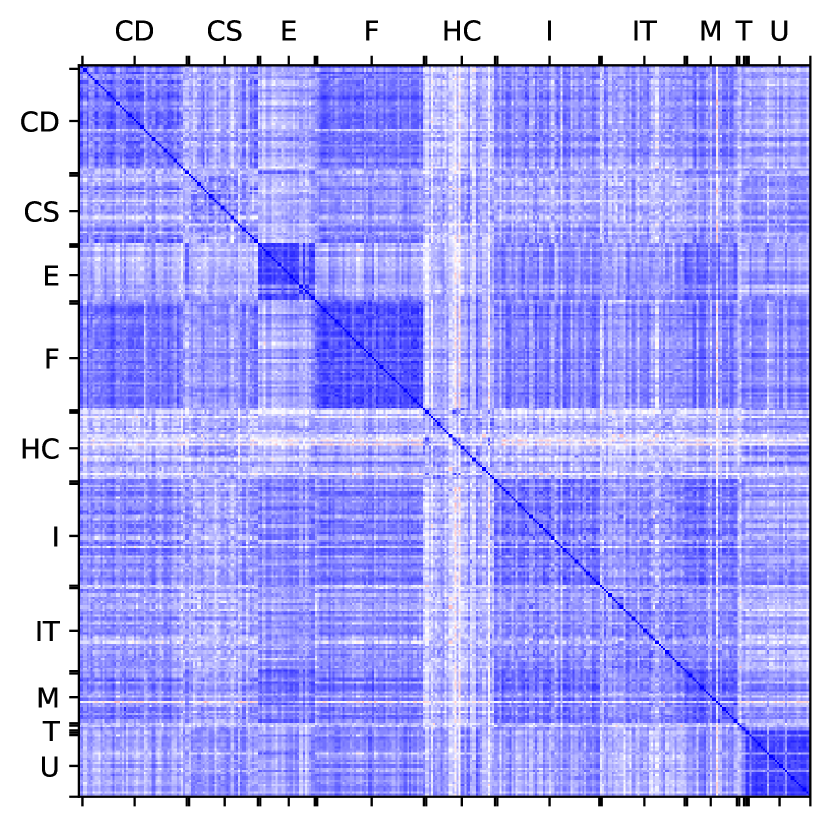
(a)

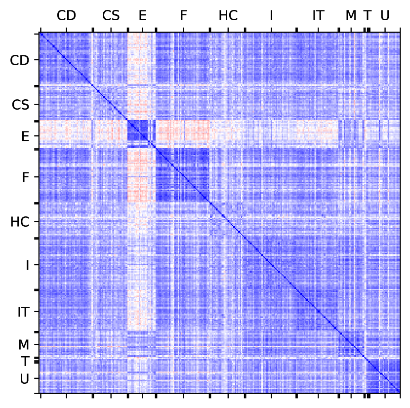
(b)

Figure 1: Correlation matrices for two subsequent epochs: daily returns of 308 stocks from the S&P 500 index. First quarter 2008 (a), second quarter 2008 (b), ordered according to industrial sectors [55]. Color coding from dark blue over white to red indicating positive, zero and negative correlation coefficients. Industrial sectors: Consumer Discretionary (CD), Consumer Staples (CS), Energy (E), Financials (F), Health Care (HC), Industrials (I), Information Technology (IT), Materials (M), Telecommunications Services (T), Utilities (U).

structures due to the industrial sectors remain largely unchanged, the two correlation matrices are clearly different.

This prompts us to treat non–stationarity of complex system in general in the following way. To model multivariate distributions of $K$ amplitudes $r_{k},\ k=1,\ldots,K$ ordered in a vector $r=(r_{1},\ldots,r_{K})$ on a long time interval, we account for fluctuating correlations by separating the time scales as in Fig. 2.

Figure 2: Long interval, divided into epochs.

We divide the long time interval into short epochs on which we assume only small variations of the correlations. Conceptually, we may even drop this assumption, although it provides a convenient guideline for a data analysis. All what matters is that in our model we view the fluctuations of the correlations on the long time interval as pieced together from the individual epochs. Naturally, the multivariate distribution in the epochs on the one hand and on the long time interval on the other hand ought to be clearly different. In our model, developed in Ref. [35, 42] and further extended in Ref. [42], we make the assumption that the multivariate amplitude distributions in the different epochs have the same shape, i.e. the same functional form, and differ only in the measured correlation matrices $C_{\mathrm{ep}}$. The challenge is to choose a functional form for $p(r|C_{\mathrm{ep}})$ that properly fits the data in all epochs such that the non–stationary variations are captured by the correlation matrix $C_{\mathrm{ep}}$ which differs from epoch to epoch. The set of correlation matrices $C_{\mathrm{ep}}$ measured in all epochs is a truly existing ensemble which we now model by an ensemble of random correlation matrices $XX^{\dagger}/N$. The model data matrices $X$ have dimension $K\times N$ where $N$ is the length of the model time series. For each value of $N$, the matrices $XX^{\dagger}/N$ have dimension $K\times K$, which allows us to use $N$ as a tunable parameter. As will become clearer later on, the larger $N$, the smaller the fluctuations of the model correlations. We draw $X$ from a random matrix distribution $w(X|C,D)$. Here, $C$ and $D$ are the sample correlation matrices for time and position series, respectively, measured over the long time interval. To construct the multivariate amplitude distribution on the long time interval, we replace in $p(r|C_{\mathrm{ep}})$ the epoch correlation matrices by the random ones,

$$C_{\mathrm{ep}}\longrightarrow\frac{1}{N}XX^{\dagger}\ ,$$ (I.1)

and integrate over the ensemble

$$\langle p\rangle(r|C,D)=\int p\left(r\bigg{|}\frac{1}{N}XX^{\dagger}\right)w(X|C,D)d[X]\ ,$$ (I.2)

where the measure $d[X]$ is the product of the differentials of all independent variables, see Ref. [42]. This ensemble random matrix average is meant to capture a truly existing matrix ensemble, namely that of the epoch correlation matrices $C_{\mathrm{ep}}$, while most other random matrix models are based on the concept of second ergodicity, i.e. to model statistical features of one large spectrum, an average over a fictitious ensemble of random matrices is employed. Hence, as our random matrix model does not ground on second ergodicity, the dimension of the correlation matrices considered does not have to be large either. Our model applies to correlation matrices of any size.

2.2 Rotation and aggregation procedure

To make data analyses feasible, we will restrict the choices for $p(r|C_{\mathrm{ep}})$ and $w(X|C,D)$ such that $p(r|C_{\mathrm{ep}})$ and $\langle p\rangle(r|C,D)$ depend on the amplitudes only via the squared Mahalanobis distances [56] $r^{\dagger}C^{-1}_{\mathrm{ep}}r$ and $r^{\dagger}C^{-1}r$, respectively. The diagonalization of the correlation matrix $C$ reads

$$C=U\Lambda U^{\dagger}\qquad\mathrm{with}\qquad\Lambda=\mathrm{diag}(\Lambda_{1},\ldots,\Lambda_{K})\ ,\quad\Lambda_{k}>0$$ (I.3)

with an an orthogonal matrix $U$. The same applies to $C_{\mathrm{ep}}$ with eigenvalues $\Lambda_{\mathrm{ep},k}$. For the inverse correlation matrices, we then have $C^{-1}=U\Lambda^{-1}U^{\dagger}$. In the data analyses, we will always work with full–rank correlation matrices which warrants the existence of their inverse. For the squared Mahalanobis distance, we find

$$r^{\dagger}C^{-1}r=r^{\dagger}U\Lambda^{-1}U^{\dagger}r=\bar{r}^{\dagger}\Lambda^{-1}\bar{r}=\sum_{k=1}^{K}\frac{\bar{r}_{k}^{2}}{\Lambda_{k}}$$ (I.4)

with

$$\bar{r}=U^{\dagger}r\ ,\qquad\bar{r}_{k}=\sum_{l=1}^{K}U_{lk}r_{l}$$ (I.5)

and similarly for $C_{\mathrm{ep}}$. Thus, going from the amplitudes $r$ to the linear combinations $\bar{r}$, we rotate into the eigenbasis of the correlation matrix. If the covariance matrices are used instead of the correlation matrices, everything works in the same way mutatis mutandis. Integrating out all variables in $\bar{r}$ but one $\bar{r}_{k}$, say, we obtain $K$ univariate amplitude distributions

$$\hskip 15.6491ptp^{(\mathrm{rot},k)}(\bar{r}_{k}|C_{\mathrm{ep}}) =\int p(\bar{r}|C_{\mathrm{ep}})d[\bar{r}]_{\neq k}$$

$$\langle p\rangle^{(\mathrm{rot},k)}(\bar{r}_{k}|C,D) =\int\langle p\rangle(\bar{r}|C,D)d[\bar{r}]_{\neq k}$$ (I.6)

for each epoch and for the longer interval, respectively. The integrals are best carried out by inserting the characteristic functions. The distributions $p^{(\mathrm{rot},k)}(\bar{r}_{k}|C_{\mathrm{ep}})$ have the same functional form for all $k$ in each epoch and, similarly, the distributions $\langle p\rangle^{(\mathrm{rot},k)}(\bar{r}_{k}|C,D)$ for all $k$ on the long interval. However, their parameters, more precisely, the eigenvalues entering, are different. These $K$ distributions provide full information on the correlated multivariate system, because all linear combinations differ.

The calculation also reveals that the resulting univariate distributions for the rotated amplitudes have the same functional form as the univariate distributions $p^{(\mathrm{orig},k)}(r_{k}|C_{\mathrm{ep}})$ and $\langle p\rangle^{(\mathrm{orig},k)}(r_{k}|C,D)$ for the unrotated, original amplitudes, but of course with changes in the parametrical dependence, see Secs. 2.3 and 2.4.

Anticipating the forthcoming data analysis, we briefly sketch the procedure of aggregation. To accumulate data for statistical significance, we normalize the $\bar{r}_{k}$ to the square root of the corresponding eigenvalue,

$$\widetilde{r}_{k}=\frac{\bar{r}_{k}}{\sqrt{\Lambda_{k}}},$$ (I.7)

or $\Lambda_{\mathrm{ep},k}$, respectively, and lump together all $K$ distributions. This yields statistically highly significant univariate empirical distributions $p^{(\mathrm{aggr})}(\widetilde{r})$ and $\langle p\rangle^{(\mathrm{aggr})}(\widetilde{r})$ which facilitates a careful study of the tail behavior.

2.3 Choice of multivariate amplitude distributions in the epochs

We choose two functional forms for the amplitude distributions in the epochs. We make the assumption that non–Markovian effects may be neglected on shorter time scales, i.e. in the epochs. Their inclusion would be mathematical feasible, but would lead to much more complicated formulae. In most complex systems that we have worked with, a wise choice of the epoch length can always justify the neglection of non–Markovian effects within the epochs. We notice that short–term memory effects are known to exist in correlated financial markets [57, 58, 59, 60], but they are small. A first choice or the multivariate amplitude distributions is the Gaussian

$$p_{\mathrm{G}}(r|C_{\mathrm{ep}})=\frac{1}{\sqrt{\mathrm{det}2\pi C_{\mathrm{ep}}}}\exp{\left(-\frac{1}{2}r^{\dagger}C_{\mathrm{ep}}^{-1}r\right)}.$$ (I.8)

The measured correlation matrix

$$C_{\mathrm{ep}}=\langle rr^{\dagger}\rangle_{\mathrm{ep}}$$ (I.9)

differs from epoch to epoch. The rotated univariate amplitude distributions are

$$p_{\mathrm{G}}^{(\mathrm{rot},k)}(\bar{r}_{k}|\Lambda_{\mathrm{ep},k})=\frac{1}{\sqrt{2\pi\Lambda_{\mathrm{ep},k}}}\exp\left(-\frac{\bar{r}_{k}^{2}}{2\Lambda_{\mathrm{ep},k}}\right).$$ (I.10)

If the covariance matrices $\Sigma_{\mathrm{ep}}$ instead of the correlation matrices $C_{\mathrm{ep}}$ are used, the $\Lambda_{\mathrm{ep},k}$ are the eigenvalues of the former.

The univariate distributions of the original (unrotated) amplitudes can also be heavy-tailed for various reasons, see finance [61, 62, 63, 64, 65] as an example. This prompts our second choice [42]

$$p_{\mathrm{A}}(r|\hat{C}_{\mathrm{ep}})=\sqrt{\frac{2}{m}}^{K}\frac{\Gamma(l-(K-1)/2)}{\Gamma(l-K/2)}\frac{1}{\sqrt{\det 2\pi\hat{C}_{\mathrm{ep}}}}\frac{1}{\displaystyle\left(1+\frac{1}{m}r^{\dagger}\hat{C}^{-1}_{\mathrm{ep}}r\right)^{l}}$$ (I.11)

with an algebraic tail determined by the power $l$. We notice that the input matrix $\hat{C}_{\mathrm{ep}}$ which is to be measured for each epoch can in this algebraic case not directly be identified with the sample correlation or covariance matrix. However, the simple relation [42]

$$C_{\mathrm{ep}}=\langle rr^{\dagger}\rangle_{\mathrm{ep}}=\beta_{\mathrm{A}}\hat{C}_{\mathrm{ep}}$$ (I.12)

with

$$\beta_{\mathrm{Y}}=\cases{\displaystyle 1\ ,&if \ Y=G\\ \displaystyle\frac{m}{2l-K-2}\ ,&if \ Y=A}\ .$$ (I.13)

holds for the expectation value $\langle rr^{\dagger}\rangle$ as an estimator for the sample correlations or covariances.

Importantly, the relation (I.12) allows us to fix one of the two parameters $l$ or $m$ in this algebraic case $\mathrm{Y=A}$. We choose the latter and replace $m\hat{C}_{\mathrm{ep}}$ with $(2l-K-2)C_{\mathrm{ep}}$ such that

$$p_{\mathrm{A}}(r|C_{\mathrm{ep}}) =\sqrt{\frac{2}{2l-K-2}}^{K}\frac{\Gamma(l-(K-1)/2)}{{\Gamma(l-K/2)}}$$ (I.14)

$$\qquad\frac{1}{\sqrt{\det 2\pi C_{\mathrm{ep}}}}\frac{1}{\displaystyle\left(1+\frac{1}{2l-K-2}r^{\dagger}C_{\mathrm{ep}}^{-1}r\right)^{l}}\ .$$

In this multivariate distribution, $l$ is the only fit parameter.

Viewed as function of the Mahalanobis distance $\sqrt{r^{\dagger}\hat{C}^{-1}_{\mathrm{ep}}r}$, the distribution (I.11) is of a generalized Student $t$ type [66]. In the standard univariate Student $t$ distribution with $m$ degrees of freedom, one has $l=(m+1)/2$. Multivariate $t$ distributions were considered for financial data in Refs. [67, 68, 69] and particularly in Ref. [70]. In such $K$ multivariate $t$ distributions, with $m$ degrees of freedom, the relation $l=(m+K)/2$ holds. In our choice, the two parameters $l$ and $m$ are first independent and then related (I.12), (I.13). The $K$ multivariate distribution (I.11) is normalizable, if $l>K/2$.

Analogously to Eq. (I.10), we calculate the univariate distributions for the rotated amplitudes and find, not surprisingly, a formulae with a reduced power

$$p_{\mathrm{A}}^{(\mathrm{rot},k)}(\bar{r}_{k}|\Lambda_{\mathrm{ep},k}) =\frac{1}{\sqrt{\pi(2l_{\mathrm{rot}}-3)\Lambda_{\mathrm{ep},k}}}\frac{\Gamma(l_{\mathrm{rot}})}{\Gamma(l_{\mathrm{rot}}-1/2)}$$

$$\qquad\frac{1}{\displaystyle\left(1+\frac{\bar{r}_{k}^{2}}{(2l_{\mathrm{rot}}-3)\Lambda_{\mathrm{ep},k}}\right)^{l_{\mathrm{rot}}}}\ .$$

The combined parameter

$$l_{\mathrm{rot}}=l-\frac{K-1}{2}$$ (I.16)

occurs because we integrated out $K-1$ variables of the $K$ multivariate distribution. We notice that the $\Lambda_{\mathrm{ep},k}$ are the eigenvalues of the sample correlation matrix.

Importantly, the corresponding univariate distributions $p_{\mathrm{Y}}^{(\mathrm{orig},k)}(r_{k}|C_{\mathrm{ep}})$ for the original, unrotated amplitudes have the same functional forms. They follow from Eqs. (I.10) and (2.3) by simply replacing $\Lambda_{\mathrm{ep},k}$ with the number one or with the variances $\Sigma_{\mathrm{ep},kk}=\sigma_{\mathrm{ep},k}^{2}$ if correlation or covariance matrices are used, respectively. The information on the multivariate, correlated system is contained in the eigenvalues of the correlation or covariance matrices which appear explicitly in the univariate distributions of the rotated amplitudes, but not in those of the original, unrotated amplitudes. Hence the latter do not carry information on the multivariate, correlated system, in contrast to the former.

2.4 Choice of ensembles for the fluctuating correlations

To capture the non–stationarity, we model the fluctuations of correlations by random $K\times N$ data matrices $X$ which we draw from either Gaussian or algebraic distributions. Our first choice for the ensemble distribution is the multimultivariate Gaussian

$$w_{\mathrm{G}}(X|C,D)=\frac{1}{\sqrt{\mathrm{det}2\pi D\otimes C}}\exp{\left(-\frac{1}{2}\mathrm{tr}D^{-1}X^{\dagger}C^{-1}X\right)}\ .$$ (I.17)

In statistical inference, this is the celebrated doubly correlated Wishart distribution with input matrices $C$ and $D$ describing the correlation structure of the time and position series, $r(t)$ and $\widetilde{r}_{k}$, respectively. They can be determined by sampling over the long time interval,

$$C=\langle rr^{\dagger}\rangle\qquad\mathrm{and}\qquad D=\langle\widetilde{r}\widetilde{r}^{\dagger}\rangle\ ,$$ (I.18)

where $D$ measures the memory effects. In our model these are the non-Markovian effects across epochs. The random data matrix in the model has dimension $K\times N$, thus the time series have length $N$ which is an adjustable parameter controlling how strongly the $K\times K$ model correlation matrix $XX^{\dagger}/N$ and the $K\times K$ model correlation matrix $X^{\dagger}X/K$ fluctuate about the input matrices $C$ and $D$, respectively. Thus, it is a feature of our model that the length $N$ of the random model time series is different from, in general much shorter than, the length $T$ of the long interval. Although the input matrix $D$ in Eq. (I.17) and the sampled correlation matrix $D$ in (I.18) are different due to the structure of our model, we do not distinguish them in the notation. From a practical point of view, the input matrix $D$ should contain the sector of the sampled matrix $D$ corresponding to the largest eigenvalues.

As explained in Sec. 2.1, our model is quite different from statistical inference, second ergodicity is not evoked as the random ensemble (I.17) models the truly existing ensemble of the measured epoch correlation matrices $C_{\mathrm{ep}}$. Hence, the $K\times K$ model correlation matrices $XX^{\dagger}/N$ do not have to be large.

To model possible heavy tails in the fluctuations of the correlations, we also choose the multimultivariate, algebraic determinant distribution

$$w_{\mathrm{A}}(X|\hat{C},\hat{D}) =\left(\frac{2}{M}\right)^{\frac{KN}{2}}\prod_{n=1}^{N}\frac{\Gamma(L-(n-1)/2)}{\Gamma(L-(K+n-1)/2)}\frac{1}{\sqrt{\mathrm{det}2\pi\hat{D}\otimes\hat{C}}}$$ (I.19)

$$\qquad\qquad\qquad\qquad\frac{1}{\displaystyle\mathrm{det}^{L}\left(\mathbb{1}_{N}+\frac{1}{M}\hat{D}^{-1}X^{\dagger}\hat{C}^{-1}X\right)}$$

depending on two input parameter correlation matrices $\hat{C}$ and $\hat{D}$. It generalizes the matrixvariate $t$ distribution with $\nu$ degrees of freedom [45] which is recovered for $M=1$ and $L=(\nu+K+N-1)/2$. In our application, $L,M,N$ are first independent parameters, but the relations [42]

$$C=B_{\mathrm{A}}\hat{C}\qquad\mathrm{and}\qquad D=B_{\mathrm{A}}\hat{D}$$ (I.20)

between the sample and the input parameter correlation matrices with

$$B_{\mathrm{Y}}=\cases{\displaystyle 1\ ,&if \ Y=G\\ \displaystyle\frac{M}{2L-K-N-1}\ ,&if \ Y=A}\ .$$ (I.21)

facilitates the elimination of the parameter $M$. In Eq. (I.19), we replace $M\hat{C}$ with $(2L-K-N-1)C$ and find

$$w_{\mathrm{A}}(X|C,D) =\left(\frac{2}{2L-K-N-1}\right)^{\frac{KN}{2}}$$ (I.22)

$$\qquad\prod_{n=1}^{N}\frac{\Gamma(L-(n-1)/2)}{\Gamma(L-(K+n-1)/2)}\frac{1}{\sqrt{\mathrm{det}2\pi D\otimes C}}$$

$$\qquad\qquad\frac{1}{\displaystyle\mathrm{det}^{L}\left(\mathbb{1}_{N}+\frac{1}{2L-K-N-1}D^{-1}X^{\dagger}C^{-1}X\right)}\ .$$

Importantly, as the dependence of $w_{\mathrm{A}}(X|\hat{C},\hat{D})$ on the input matrices $\hat{C}$ and $\hat{D}$ is, apart from their dimensions, fully symmetric, the replacements of $M\hat{C}$ with $(2L-K-N-1)C$ and of $M\hat{D}$ with $(2L-K-N-1)D$ are equivalent. Hence the ensemble averages $\langle XX^{\dagger}/N\rangle$ and $\langle X^{\dagger}X/K\rangle$ now yield $C$ and $D$ as required.

2.5 Resulting multivariate amplitude distributions on the long interval

Employing Eq. (I.2), we calculate the multivariate amplitude distributions $\langle p\rangle_{YY^{\prime}}(r|C,D)$ on the long interval. As the multivariate amplitude distributions $p_{\mathrm{Y}}(r|C_{\mathrm{ep}})$ and the ensemble distributions $w_{\mathrm{Y^{\prime}}}(X|C,D)$ both come in a Gaussian $\mathrm{Y=G}$ and an algebraic $\mathrm{Y=A}$ choice according to Eqs. (I.8), (I.11), (I.17), (I.19), we arrive at four distributions $\langle p\rangle_{YY^{\prime}}(r|C,D)$ on the long interval. Details of the calculations can be found in Ref. [42], we only present the results. Remarkably, almost all integrals can be done, the formulae are fairly compact, given the complexity of the model. It is an important feature of our model, that all multivariate distribution on the long interval depend on the amplitudes only via the Mahalanobis distances [56] $\sqrt{r^{\dagger}C^{-1}r}$. Explicitly, our results are

$$\langle p\rangle_{\mathrm{GG}}(r|C,D) =\frac{1}{\sqrt{r^{\dagger}C^{-1}r}^{(K-2)/2}}\frac{1}{\sqrt{\det 2\pi C}}$$ (I.23)

$$\qquad\int\limits_{0}^{\infty}\frac{J_{(K-2)/2}\left(\rho\sqrt{r^{\dagger}C^{-1}r}\right)}{\sqrt{\det(\mathbb{1}_{N}+D\rho^{2}/N)}}\rho^{K/2}d\rho$$

in the Gaussian–Gaussian case,

$$\langle p\rangle_{\mathrm{GA}}(r|C,D) =\frac{\Gamma(L-(N-1)/2)}{\Gamma(K/2)\Gamma(L-(K-N-1)/2)}$$ (I.24)

$$\qquad\frac{1}{\sqrt{\det 2\pi C(2L-K-N-1)/N}}$$

$$\qquad\qquad\int\limits_{0}^{\infty}{{}_{1}F_{1}}\bigg{(}L-\frac{N-1}{2},\frac{K}{2},$$

$$\qquad\qquad\qquad-\frac{uN}{2(2L-K-N-1)}r^{\dagger}C^{-1}r\bigg{)}$$

$$\qquad\qquad\qquad\qquad\frac{u^{K/2-1}du}{\sqrt{\det(\mathbb{1}_{N}+uD)}}$$

in the Gaussian-Algebraic case,

$$\langle p\rangle_{\mathrm{AG}}(r|C,D) =\frac{\Gamma(l)}{\Gamma(K/2)\Gamma(l-K/2)}\frac{1}{\sqrt{\det 2\pi C(2l-K-2)/N}}$$ (I.25)

$$\qquad\int\limits_{0}^{\infty}{{}_{1}F_{1}}\left(l,\frac{K}{2},-\frac{uN}{2(2l-K-2)}r^{\dagger}C^{-1}r\right)$$

$$\qquad\qquad\frac{u^{K/2-1}du}{\sqrt{\det(\mathbb{1}_{N}+uD)}}$$

in the Algebraic–Gaussian case and finally

$$\langle p\rangle_{\mathrm{AA}}(r|C,D) =\frac{\Gamma(l)\Gamma(l-(N-1)/2)}{\Gamma(K/2)\Gamma(l-K/2)\Gamma(L-(K+N-1)/2)}$$ (I.26)

$$\qquad\frac{1}{\sqrt{\det 2\pi C(2l-K-2)(2L-K-N-1)/N}}$$

$$\qquad\int\limits_{0}^{\infty}{{}_{2}F_{1}}\bigg{(}l,L-\frac{N-1}{2},\frac{K}{2},$$

$$\qquad\qquad-\frac{uN}{(2l-K-2)(2L-K-N-1)}r^{\dagger}C^{-1}r\bigg{)}$$

$$\qquad\qquad\qquad\frac{u^{K/2-1}du}{\sqrt{\det(\mathbb{1}_{N}+uD)}}$$

in the Algebraic–Algebraic case. For the occurring special functions Bessel $J_{\nu}$, Macdonald $K_{\nu}$, Kummer ${}_{1}F_{1}$, Tricomi $U$ and hypergeometric Gauss ${}_{2}F_{1}$ we use the definitions and conventions of Ref. [71]. These multivariate distributions $\langle p\rangle_{\mathrm{YY^{\prime}}}(r|C,D)$ still include non–Markovian effects encoded in the input correlation matrix $D$ of the position series. We notice that only its eigenvalues enter the multivariate distributions. A thorough study of memory effects in the context of our model should be carried out in systems such as climate or traffic where their role can be clearly distinguished. The Markovian case $D=\mathbb{1}_{N}$ is of particular interest.

We derive the univariate distributions of the rotated amplitudes $\bar{r}_{k}$, calculate the integrals over the other $K-1$ rotated amplitudes, define the combined parameter

$$L_{\mathrm{{rot}}}=L-\frac{K-1}{2}$$ (I.27)

analogously to $l_{\mathrm{rot}}$ in Eq. (I.16) and arrive at

$$\langle p\rangle_{\mathrm{GG}}^{(\mathrm{rot},k)}(\bar{r}_{k}|\Lambda_{k}) =\frac{1}{2^{(N-1)/2}\Gamma(N/2)}\sqrt{\frac{N}{\pi\Lambda_{k}}}\left(\frac{N\bar{r}^{2}}{\Lambda_{k}}\right)^{(N-1)/4}$$ (I.28)

$$\qquad K_{(1-N)/2}\left(\sqrt{\frac{N\bar{r}^{2}}{\Lambda_{k}}}\right)$$

in the Gaussian–Gaussian case,

$$\langle p\rangle_{\mathrm{GA}}^{(\mathrm{rot},k)}(\bar{r}_{k}|\Lambda_{k}) =\frac{\Gamma(L_{\mathrm{rot}}-(N-1)/2)\Gamma(L_{\mathrm{rot}})}{\Gamma(L_{\mathrm{rot}}-N/2)\Gamma(N/2)}$$ (I.29)

$$\qquad\sqrt{\frac{N}{2\pi(2L_{\mathrm{rot}}-N-2)\Lambda_{k}}}U\bigg{(}L_{\mathrm{rot}}-\frac{N-1}{2},$$

$$\qquad\qquad\qquad\frac{1-N}{2}+1,\frac{N\bar{r}^{2}}{2(2L_{\mathrm{rot}}-N-2)\Lambda_{k}}\bigg{)}$$

in the Gaussian–Algebraic case,

$$\langle p\rangle_{\mathrm{AG}}^{(\mathrm{rot},k)}(\bar{r}_{k}|\Lambda_{k}) =\frac{\Gamma(l_{\mathrm{rot}})\Gamma(l_{\mathrm{rot}}+(N-1)/2)}{\Gamma(l_{\mathrm{rot}}-1/2)\Gamma(N/2)}$$ (I.30)

$$\qquad\sqrt{\frac{N}{2\pi(2l_{\mathrm{rot}}-3)\Lambda_{k}}}$$

$$\qquad\qquad U\left(l_{\mathrm{rot}},\frac{1-N}{2}+1,\frac{N\bar{r}_{k}^{2}}{2(2l_{\mathrm{rot}}-3)\Lambda_{k}}\right)$$

in the Algebraic–Gaussian case and finally

$$\langle p\rangle_{\mathrm{AA}}^{(\mathrm{rot},k)}(\bar{r}_{k}|\Lambda_{k}) =\frac{\Gamma(l_{\mathrm{rot}})\Gamma(l_{\mathrm{rot}}+(N-1)/2)}{\Gamma(L_{\mathrm{rot}}-1/2)\Gamma(L_{\mathrm{rot}}+l_{\mathrm{rot}})}$$ (I.31)

$$\qquad\frac{\Gamma(L_{\mathrm{rot}})\Gamma(L_{\mathrm{rot}}-(N-1)/2)}{\Gamma(L_{\mathrm{rot}}-N/2)\Gamma(N/2)}$$

$$\qquad\qquad\sqrt{\frac{N}{\pi(2L_{\mathrm{rot}}-N-2)(2l_{\mathrm{rot}}-3)\Lambda_{k}}}$$

$$\qquad\qquad{}_{2}F_{1}\bigg{(}l_{\mathrm{rot}},L_{\mathrm{rot}}-\frac{N-1}{2},L_{\mathrm{rot}}+l_{\mathrm{rot}},$$

$$\qquad\qquad\qquad 1-\frac{N\bar{r}_{k}^{2}}{(2L_{\mathrm{rot}}-N-2)(2l_{\mathrm{rot}}-3)\Lambda_{k}}\bigg{)}$$

in the Algebraic–Algebraic case. The same remark as for univariate distributions on the epochs applies. The corresponding univariate distributions $\langle p\rangle_{\mathrm{YY^{\prime}}}^{(\mathrm{orig},k)}(r_{k}|\Lambda_{k})$ for the original, unrotated amplitudes $r_{k}$ have the same functional form. They follow from the above formulae by simply replacing $\Lambda_{k}$ with the number one or with the variances $\Sigma_{kk}=\sigma_{k}^{2}$ if correlation or covariance matrices are used, respectively. Importantly, the equality of the functional forms for the univariate distributions of original and rotated amplitudes does not mean that the latter ones do not carry new information on the multivariate system. The opposite is true. This information is encoded in the eigenvalues of the correlation or covariance matrices which enter the univariate distributions of the rotated amplitudes. Information on the multivariate system can never be retrieved from only knowing the univariate distributions of the original amplitudes.

Which are the parameters to be fitted in the above given univariate distributions on the long interval? Of course, the number $K$ of stocks, the sample correlation matrix $C$ and its eigenvalues $\Lambda_{k}$ are known. The parameter $l$ or, equivalently, $l_{\mathrm{rot}}$ has been determined by the fits of the epoch distributions. Hence, for all distributions on the long interval, $N$ is a fit parameter and in the Gaussian–Algebraic and the Algebraic–Algebraic cases, $L$ or, equivalently, $L_{\mathrm{rot}}$ is a second fit parameter.

We notice that due to our construction, the variances of the univariate distributions for the rotated amplitudes are given [42] by

$$\langle\bar{r}_{k}^{2}\rangle_{\mathrm{YY^{\prime}}}^{(\mathrm{rot},k)}=\Lambda_{k}$$ (I.32)

in all four cases $\mathrm{Y,Y^{\prime}=G,A}$, where $\Lambda_{k}$ is eigenvalue of the sample correlation or covariance matrix.

2.6 Moments of the squared Mahanalobis distance

As already pointed out, the multivariate distributions in our modeling depend on the amplitudes $r$ only via the (squared) Mahalanobis distances [56] $r^{\dagger}C^{-1}_{\mathrm{ep}}r$ and $r^{\dagger}C^{-1}r$, respectively. As their moments are easily empirically analyzed, it is useful for the data analysis to calculate them in the framework of our model. Every multivariate distribution on the long interval depending on the amplitudes $r$ has the form $f\left(r^{\dagger}C^{-1}r\right)/\sqrt{\det C}$. Thus, the $\nu$–th moment of the squared Mahalanobis distance is given by

$$\bigl{\langle}(r^{\dagger}C^{-1}r)^{\nu}\bigr{\rangle}=\frac{1}{\sqrt{\det C}}\int(r^{\dagger}C^{-1}r)^{\nu}f(r^{\dagger}C^{-1}r)d[r]$$ (I.33)

on the long interval and analogously on the epochs. We rewrite this as a $w$–integral over a $\delta$–function,

$$\bigl{\langle}(r^{\dagger}C^{-1}r)^{\nu}\bigr{\rangle} =\frac{1}{\sqrt{\det C}}\int d[r]\int\limits_{0}^{\infty}dw\delta(w-r^{\dagger}C^{-1}r)w^{\nu}f(w)$$ (I.34)

$$=\int\limits_{0}^{\infty}dww^{\nu}f(w)\int d[s]\delta(w-s^{2})$$

$$=\frac{\pi^{K/2}}{\Gamma(K/2)}\int\limits_{0}^{\infty}w^{K/2-1+\nu}f(w)dw\ .$$

The change of variables $r=C^{1/2}s$ is always possible because $C$ is positive definite. We further use hyperspherical coordinates and integrate over the angles which yields the surface of the unit sphere in $K$ dimensions. Importantly, the moments do not depend on the correlation matrix $C$, but they depend on $D$.

The integrals (I.34) can be done explicitly for the multivariate amplitude distributions $p_{\mathrm{Y}}(r|C_{\mathrm{ep}})$ on the epochs,

$$\bigl{\langle}(r^{\dagger}C_{\mathrm{ep}}^{-1}r)^{\nu}\bigr{\rangle}_{\mathrm{ep,G}} =\frac{2^{\nu}\Gamma(K/2+\nu)}{\Gamma(K/2)}$$

$$\bigl{\langle}(r^{\dagger}C_{\mathrm{ep}}^{-1}r)^{\nu}\bigr{\rangle}_{\mathrm{ep,A}} =\frac{(2l-K-2)^{\nu}\Gamma(K/2+\nu)\Gamma(l-K/2-\nu)}{\Gamma(K/2)\Gamma(l-K/2)}\ ,$$ (I.35)

where the condition $\nu<l-K/2$ holds in the algebraic case for convergence reasons. For the multivariate amplitude distributions $\langle p\rangle_{\mathrm{YY^{\prime}}}(r|C,D)$ on the long interval, we restrict ourselves to the Markovian case $D=\mathbb{1}_{N}$ and find

$$\bigl{\langle}(r^{\dagger}C^{-1}r)^{\nu}\bigr{\rangle}_{\mathrm{GG}} =\left(\frac{4}{N}\right)^{\nu}\frac{\Gamma(K/2+\nu)\Gamma(N/2+\nu)}{\Gamma(K/2)\Gamma(N/2)}$$

$$\bigl{\langle}(r^{\dagger}C^{-1}r)^{\nu}\bigr{\rangle}_{\mathrm{GA}} =\left(\frac{2(2L-K-N-1)}{N}\right)^{\nu}$$

$$\qquad\frac{\Gamma(K/2+\nu)\Gamma(N/2+\nu)\Gamma(L-(K+N-1)/2-\nu)}{\Gamma(K/2)\Gamma(N/2)\Gamma(L-(K+N-1)/2)}$$

$$\bigl{\langle}(r^{\dagger}C^{-1}r)^{\nu}\bigr{\rangle}_{\mathrm{AG}} =\left(\frac{2(2l-K-2)}{N}\right)^{\nu}$$

$$\qquad\frac{\Gamma(K/2+\nu)\Gamma(N/2+\nu)\Gamma(l-K/2-\nu)}{\Gamma(K/2)\Gamma(N/2)\Gamma(l-K/2)}$$

$$\bigl{\langle}(r^{\dagger}C^{-1}r)^{\nu}\bigr{\rangle}_{\mathrm{AA}} =\left(\frac{(2l-K-2)(2L-K-N-1)}{N}\right)^{\nu}$$ (I.36)

$$\qquad\frac{\Gamma(K/2+\nu)\Gamma(N/2+\nu)\Gamma(l-K/2-\nu)}{\Gamma(K/2)\Gamma(N/2)\Gamma(l-K/2)}$$

$$\qquad\qquad\frac{\Gamma(L-(K+N-1)/2-\nu)}{\Gamma(L-(K+N-1)/2)}\ ,$$

with the existence conditions $\nu<l-K/2$ and $\nu<L-(K+N-1)/2$. As these formulae involve various $\Gamma$ functions, it is helpful to introduce moment ratios of the form

$$Q^{(\nu)}=\frac{\bigl{\langle}(r^{\dagger}C^{-1}r)^{\nu}\bigr{\rangle}}{\bigl{\langle}r^{\dagger}C^{-1}r\bigr{\rangle}^{\nu}}$$ (I.37)

or similar. We consider particularly the case $\nu=2$ and arrive at

$$Q_{\mathrm{ep,G}}^{(2)} =\frac{K+2}{K}$$

$$Q_{\mathrm{ep,A}}^{(2)} =\frac{K+2}{K}\,\frac{2l-K-2}{2l-K-4}$$ (I.38)

for the epochs and at

$$Q_{\mathrm{GG}}^{(2)} =\frac{(K+2)(N+2)}{KN}$$

$$Q_{\mathrm{GA}}^{(2)} =\frac{(K+2)(N+2)}{KN}\,\frac{2L-K-N-1}{2L-K-N+1}$$

$$Q_{\mathrm{AG}}^{(2)} =\frac{(K+2)(N+2)}{KN}\,\frac{2l-K-2}{2l-K-4}$$

$$Q_{\mathrm{AA}}^{(2)} =\frac{(K+2)(N+2)}{KN}\,\frac{2L-K-N-1}{2L-K-N+1}\,\frac{2l-K-2}{2l-K-4}$$ (I.39)

for the long interval. These ratios have clear systematics and a much simpler dependence on the parameters than the moments. They are handy quantities to facilitate the parameter fixing by comparing with their empirical values. In the Gaussian–Gaussian case, $N$ is the only parameter and can be fixed either by fitting the distribution or by comparing the ratios. In the other cases, combinations of both are needed or other ratios have to be employed.

3 Conclusions

When analyzing data of complex systems, it is often a real challenge to identify the proper observables. Strong correlations are typically found between the constituents or, more precisely, the measured amplitudes. Thus, neither the data analysis nor the construction of models can only resort to univariate distributions. The situation is even more involved as non-stationarity belongs to the characterizing features of complex systems.

We presented and further extended a model for the multivariate joint probability density functions of the measured amplitudes. To this end, we gave a new interpretation for Wishart-type-of approaches. In traditional statistics, they are used for inference, while we employ them to model a truly existing ensemble of measured correlation matrices in the epochs. Choosing Gaussian and algebraic multivariate amplitude distributions in the epochs and Gaussian and algebraic distributions for the random model correlation matrices, we derive four different multivariate distributions on the long interval. Of particular interest are the tails. The non–stationarity fluctuations of the correlations lift the tails when going from epochs to the long interval. The functional form of the distribution changes, too. This main result of our model is made explicit in a variety of formulae for the data analysis which considerably extend and simplify our previous formulae. In the forthcoming study II, we apply them to a correlated financial market, further applications to other complex systems are planned.

References

- [1] Rosario N. Mantegna and H. Eugene Stanley “Introduction to Econophysics: Correlations and Complexity in Finance” Cambridge: Cambridge University Press, 1999
- [2] Ryszard Kutner et al. “Econophysics and sociophysics: Their milestones challenges” In Physica A: Statistical Mechanics and its Applications 516, 2019, pp. 240 –253 DOI: https://doi.org/10.1016/j.physa.2018.10.019
- [3] Vasiliki Plerou et al. “Random matrix approach to cross correlations in financial data” In Phys. Rev. E 65 American Physical Society, 2002, pp. 066126 DOI: 10.1103/PhysRevE.65.066126
- [4] Michael C. Münnix et al. “Identifying States of a Financial Market” In Scientific Reports 2, 2012, pp. 644 DOI: 10.1038/srep00644
- [5] Shanshan Wang, Sebastian Gartzke, Michael Schreckenberg and Thomas Guhr “Quasi-stationary states in temporal correlations for traffic systems: Cologne orbital motorway as an example” In Journal of Statistical Mechanics: Theory and Experiment 2020.10 IOP Publishing, 2020, pp. 103404 DOI: 10.1088/1742-5468/abbcd3
- [6] Shanshan Wang, Sebastian Gartzke, Michael Schreckenberg and Thomas Guhr “Collective behavior in the North Rhine-Westphalia motorway network” In Journal of Statistical Mechanics: Theory and Experiment 2021.12 IOP Publishing, 2021, pp. 123401 DOI: 10.1088/1742-5468/ac3662
- [7] Henrik M. Bette, Edgar Jungblut and Thomas Guhr “Nonstationarity in correlation matrices for wind turbine SCADA-data” In Wind Energy 26.8, 2023, pp. 826–849 DOI: https://doi.org/10.1002/we.2843
- [8] G. William Schwert “Why does stock market volatility change over time?” In The journal of finance 44.5 Wiley Online Library, 1989, pp. 1115–1153 DOI: 10.1111/j.1540-6261.1989.tb02647.x
- [9] Benoit B. Mandelbrot “”The variation of certain speculative prices”” In Fractals and Scaling in Finance: Discontinuity, Concentration, Risk. Selecta Volume E New York, NY: Springer New York, 1997, pp. 371–418 DOI: 10.1007/978-1-4757-2763-0˙14
- [10] Geert Bekaert and Guojun Wu “Asymmetric Volatility and Risk in Equity Markets” In The Review of Financial Studies 13.1, 2000, pp. 1–42 DOI: 10.1093/rfs/13.1.1
- [11] Geert Bekaert and Marie Hoerova “The VIX, the variance premium and stock market volatility” Analysis of Financial Data In Journal of Econometrics 183.2, 2014, pp. 181–192 DOI: https://doi.org/10.1016/j.jeconom.2014.05.008
- [12] Mieszko Mazur, Man Dang and Miguel Vega “COVID-19 and the march 2020 stock market crash. Evidence from S&P1500” In Finance Research Letters 38, 2021, pp. 101690 DOI: https://doi.org/10.1016/j.frl.2020.101690
- [13] Karl Pearson “X. On the criterion that a given system of deviations from the probable in the case of a correlated system of variables is such that it can be reasonably supposed to have arisen from random sampling ” In The London, Edinburgh, and Dublin Philosophical Magazine and Journal of Science 50.302 Taylor & Francis, 1900, pp. 157–175 DOI: 10.1080/14786440009463897
- [14] Abe Sklar “Fonctions de répartition à n dimensions et leurs marges” In Publ. Inst. Statist. Univ. Paris 8, 1959, pp. 229–231
- [15] Abe Sklar “Random variables, joint distribution functions, and copulas” In Kybernetika 9.6 Institute of Information TheoryAutomation AS CR, 1973, pp. 449–460
- [16] Roger B. Nelsen “An introduction to copulas” New York: Springer, 2010
- [17] Michael C. Münnix and Rudi Schäfer “A copula approach on the dynamics of statistical dependencies in the US stock market” In Physica A: Statistical Mechanics and its Applications 390.23, 2011, pp. 4251–4259 DOI: https://doi.org/10.1016/j.physa.2011.06.032
- [18] David Salinas et al. “High-dimensional multivariate forecasting with low-rank gaussian copula processes” In Advances in neural information processing systems 32, 2019
- [19] Desislava Chetalova, Rudi Schäfer and Thomas Guhr “Zooming into market states” In Journal of Statistical Mechanics: Theory and Experiment 2015.1 IOP Publishing, 2015, pp. P01029 DOI: 10.1088/1742-5468/2015/01/p01029
- [20] Desislava Chetalova, Marcel Wollschläger and Rudi Schäfer “Dependence structure of market states” In Journal of Statistical Mechanics: Theory and Experiment 2015.8 IOP Publishing, 2015, pp. P08012 DOI: 10.1088/1742-5468/2015/08/p08012
- [21] Yuriy Stepanov, Erik Wellner and Tarek Abou-Zeid “Multi-Asset Correlation Dynamics with Application to Trading” A PhD Project, 2015 DOI: 10.13140/RG.2.2.18674.56009
- [22] Yuriy Stepanov et al. “Stability and hierarchy of quasi-stationary states: financial markets as an example” In Journal of Statistical Mechanics: Theory and Experiment 2015.8 IOP Publishing, 2015, pp. P08011 DOI: 10.1088/1742-5468/2015/08/p08011
- [23] Philip Rinn et al. “Dynamics of quasi-stationary systems: Finance as an example” In EPL (Europhysics Letters) 110.6 IOP Publishing, 2015, pp. 68003 DOI: 10.1209/0295-5075/110/68003
- [24] Hirdesh K. Pharasi et al. “Identifying long-term precursors of financial market crashes using correlation patterns” In New Journal of Physics 20.10 IOP Publishing, 2018, pp. 103041 DOI: 10.1088/1367-2630/aae7e0
- [25] Anton J. Heckens, Sebastian M. Krause and Thomas Guhr “Uncovering the Dynamics of Correlation Structures Relative to the Collective Market Motion” In Journal of Statistical Mechanics: Theory and Experiment 2020.10 IOP Publishing, 2020, pp. 103402 DOI: 10.1088/1742-5468/abb6e2
- [26] Anton J. Heckens and Thomas Guhr “A new attempt to identify long-term precursors for endogenous financial crises in the market correlation structures” In Journal of Statistical Mechanics: Theory and Experiment 2022.4 IOP Publishing, 2022, pp. 043401 DOI: 10.1088/1742-5468/ac59ab
- [27] Anton J. Heckens and Thomas Guhr “New collectivity measures for financial covariances and correlations” In Physica A: Statistical Mechanics and its Applications 604, 2022, pp. 127704 DOI: https://doi.org/10.1016/j.physa.2022.127704
- [28] Gautier Marti, Frank Nielsen, Mikołaj Bińkowski and Philippe Donnat “A Review of Two Decades of Correlations, Hierarchies, Networks and Clustering in Financial Markets” In Progress in Information Geometry: Theory and Applications Cham: Springer International Publishing, 2021, pp. 245–274 DOI: 10.1007/978-3-030-65459-7˙10
- [29] Hirdesh K. Pharasi, Eduard Seligman and Thomas H. Seligman “Market states: A new understanding” arXiv:2003.07058, 2020 arXiv:2003.07058 [q-fin.CP]
- [30] Hirdesh K. Pharasi et al. “Dynamics of the market states in the space of correlation matrices with applications to financial markets” arXiv:2107.05663, 2021 arXiv:2107.05663 [q-fin.ST]
- [31] Nick James, Max Menzies and Georg A. Gottwald “On financial market correlation structures and diversification benefits across and within equity sectors” In Physica A: Statistical Mechanics and its Applications 604, 2022, pp. 127682 DOI: https://doi.org/10.1016/j.physa.2022.127682
- [32] Tobias Wand, Martin Heßler and Oliver Kamps “Identifying dominant industrial sectors in market states of the S&P 500 financial data” In Journal of Statistical Mechanics: Theory and Experiment 2023.4 IOP Publishing, 2023, pp. 043402 DOI: 10.1088/1742-5468/accce0
- [33] Martin Heßler, Tobias Wand and Oliver Kamps “Efficient Multi-Change Point Analysis to Decode Economic Crisis Information from the S&P500 Mean Market Correlation” In Entropy 25.9, 2023 DOI: 10.3390/e25091265
- [34] Tobias Wand, Martin Heßler and Oliver Kamps “Memory Effects, Multiple Time Scales and Local Stability in Langevin Models of the S&P500 Market Correlation” In Entropy 25.9, 2023 DOI: 10.3390/e25091257
- [35] Thilo A. Schmitt, Desislava Chetalova, Rudi Schäfer and Thomas Guhr “Non-stationarity in financial time series: Generic features and tail behavior” In EPL (Europhysics Letters) 103.5 IOP Publishing, 2013, pp. 58003 DOI: 10.1209/0295-5075/103/58003
- [36] Thilo A. Schmitt, Desislava Chetalova, Rudi Schäfer and Thomas Guhr “Credit risk and the instability of the financial system: An ensemble approach” In Europhysics Letters 105.3 EDP Sciences, IOP PublishingSocietà Italiana di Fisica, 2014, pp. 38004 DOI: 10.1209/0295-5075/105/38004
- [37] Thilo Schmitt, Rudi Schäfer and Thomas Guhr “Credit Risk: Taking Fluctuating Asset Correlations into Account” In Journal of Credit Risk 11.3, 2015 DOI: http://doi.org/10.21314/JCR.2015.196
- [38] Desislava Chetalova, Thilo A. Schmitt, Rudi Schäfer and Thomas Guhr “Portfolio return distributions: sample statistics with stochastic correlations” In International Journal of Theoretical and Applied Finance 18.02, 2015, pp. 1550012 DOI: 10.1142/S0219024915500120
- [39] Frederik Meudt, Martin Theissen, Rudi Schäfer and Thomas Guhr “Constructing analytically tractable ensembles of stochastic covariances with an application to financial data” In Journal of Statistical Mechanics: Theory and Experiment 2015.11 IOP PublishingSISSA, 2015, pp. P11025 DOI: 10.1088/1742-5468/2015/11/P11025
- [40] Joachim Sicking, Thomas Guhr and Rudi Schäfer “Concurrent credit portfolio losses” In PLOS ONE 13.2 Public Library of Science, 2018, pp. 1–20 DOI: 10.1371/journal.pone.0190263
- [41] Andreas Mühlbacher and Thomas Guhr “Extreme Portfolio Loss Correlations in Credit Risk” In Risks 6.3, 2018 DOI: 10.3390/risks6030072
- [42] Thomas Guhr and Andreas Schell “Exact multivariate amplitude distributions for non-stationary Gaussian or algebraic fluctuations of covariances or correlations” In Journal of Physics A: Mathematical and Theoretical 54.12 IOP Publishing, 2021, pp. 125002 DOI: 10.1088/1751-8121/abe3c8
- [43] Madan Lal Mehta “Random matrices and the statistical theory of energy levels” New York: Acad. Press, 1967
- [44] Thomas Guhr, Axel Müller–Groeling and Hans A. Weidenmüller “Random–matrix theories in quantum physics: common concepts” In Physics Reports 299.4, 1998, pp. 189–425 DOI: https://doi.org/10.1016/S0370-1573(97)00088-4
- [45] A.K. Gupta and D.K. Nagar “Matrix Variate Distributions”, Monographs and Surveys in Pure and Applied Mathematics 104 Chapman Hall/CRC, 2000 URL: https://books.google.de/books?id=Kp3Nx03\_gMwC
- [46] Marc Potters and Jean-Philippe Bouchaud “A first course in random matrix theory for physicists, engineers and data scientists” Cambridge, United Kingdom: Cambridge Universty Press, 2021 DOI: 10.1017/9781108768900
- [47] Satya D. Dubey “Compound gamma, beta and F distributions” In Metrika 16.1, 1970, pp. 27–31 DOI: 10.1007/BF02613934
- [48] O. Barndorff-Nielsen, J. Kent and M. Sørensen “Normal Variance-Mean Mixtures and z Distributions” In International Statistical Review / Revue Internationale de Statistique 50.2 [Wiley, International Statistical Institute (ISI)], 1982, pp. 145–159 URL: http://www.jstor.org/stable/1402598
- [49] O. Barndorff-Nielsen, J. Kent and M. Sørensen “Normal Variance-Mean Mixtures and z Distributions” Full publication date: Aug., 1982 In International Statistical Review / Revue Internationale de Statistique 50.2 [Wiley, International Statistical Institute (ISI)], 1982, pp. 145–159 DOI: 10.2307/1402598
- [50] Christian Beck and Ezechiel G. D. Cohen “Superstatistics” In Physica A: Statistical Mechanics and its Applications 322, 2003, pp. 267–275 DOI: https://doi.org/10.1016/S0378-4371(03)00019-0
- [51] Ashraf A. Abul-Magd, Gernot Akemann and Pierpaolo Vivo “Superstatistical generalizations of Wishart–Laguerre ensembles of random matrices” In Journal of Physics A: Mathematical and Theoretical 42.17, 2009, pp. 175207 DOI: 10.1088/1751-8113/42/17/175207
- [52] Anthony P. Doulgeris and Torbjørn Eltoft “Scale Mixture of Gaussian Modelling of Polarimetric SAR Data” In EURASIP Journal on Advances in Signal Processing 2010.1, 2009, pp. 874592 DOI: 10.1155/2010/874592
- [53] Florence Forbes and Darren Wraith “A new family of multivariate heavy-tailed distributions with variable marginal amounts of tailweight: application to robust clustering” In Statistics and Computing 24.6, 2014, pp. 971–984 DOI: 10.1007/s11222-013-9414-4
- [54] Anton J. Heckens, Efstratios Manolakis and Thomas Guhr “Multivariate Distributions in Non–Stationary Complex Systems II: Empirical Results for Correlated Stock Markets” submitted for publication (2024).
- [55] MSCI, S&P Dow Jones Indices LLC and its affiliates “Global Industry Classification Sector (GICS)” MSCI, 2023
- [56] “Reprint of: Mahalanobis, P.C. (1936) ”On the Generalised Distance in Statistics.”” In Sankhya A 80, 2018, pp. 1–7 URL: https://api.semanticscholar.org/CorpusID:239595337
- [57] Shanshan Wang, Rudi Schäfer and Thomas Guhr “Price response in correlated financial markets: empirical results” arXiv:1510.03205, 2016 arXiv:1510.03205 [q-fin.ST]
- [58] Shanshan Wang, Rudi Schäfer and Thomas Guhr “Cross-response in correlated financial markets: individual stocks” In The European Physical Journal B 89 Springer, 2016, pp. 1–16 DOI: https://doi.org/10.1140/epjb/e2016-60818-y
- [59] Shanshan Wang, Rudi Schäfer and Thomas Guhr “Average cross-responses in correlated financial markets” In The European Physical Journal B 89 Springer, 2016, pp. 1–13 DOI: https://doi.org/10.1140/epjb/e2016-70137-0
- [60] Michael Benzaquen, Iacopo Mastromatteo, Zoltan Eisler and Jean-Philippe Bouchaud “Dissecting cross-impact on stock markets: An empirical analysis” In Journal of Statistical Mechanics: Theory and Experiment 2017.2 IOP Publishing, 2017, pp. 023406 DOI: 10.1088/1742-5468/aa53f7
- [61] R. Cont “Empirical properties of asset returns: stylized facts and statistical issues” In Quantitative Finance 1.2 Informa UK Limited, 2001, pp. 223–236 DOI: 10.1080/713665670
- [62] Xavier Gabaix, Parameswaran Gopikrishnan, Vasiliki Plerou and H. Eugene Stanley “A theory of power-law distributions in financial market fluctuations” In Nature 423.6937, 2003, pp. 267–270 DOI: 10.1038/nature01624
- [63] J. Doyne Farmer et al. “What really causes large price changes?” In Quantitative Finance 4.4 Routledge, 2004, pp. 383–397 DOI: 10.1080/14697680400008627
- [64] J. Doyne Farmer and Fabrizio Lillo “On the origin of power–law tails in price fluctuations” In Quantitative Finance 4.1 Routledge, 2004, pp. 7–11 DOI: 10.1088/1469-7688/4/1/C01
- [65] Thilo A. Schmitt, Rudi Schäfer, Michael C. Münnix and Thomas Guhr “Microscopic understanding of heavy-tailed return distributions in an agent-based model” In Europhysics Letters 100.3 EDP Sciences, IOP PublishingSocietà Italiana di Fisica, 2012, pp. 38005 DOI: 10.1209/0295-5075/100/38005
- [66] Panayiotis Theodossiou “Financial data and the skewed generalized t distribution” In Management science 44.12-part-1 INFORMS, 1998, pp. 1650–1661
- [67] Siddhartha Chib, Ram Tiwari and Sreenivasa Jammalamadaka “Bayes prediction in regressions with elliptical errors” In Journal of Econometrics 38, 1988, pp. 349–360 DOI: 10.1016/0304-4076(88)90050-4
- [68] Bernard M.S. Van Praag and Bertram M. Wesselman “Elliptical multivariate analysis” In Journal of Econometrics 41.2, 1989, pp. 189–203 DOI: https://doi.org/10.1016/0304-4076(89)90093-6
- [69] Jacek Osiewalski and Mark F.J. Steel “Bayesian marginal equivalence of elliptical regression models” In Journal of Econometrics 59.3, 1993, pp. 391–403 DOI: https://doi.org/10.1016/0304-4076(93)90032-Z
- [70] Raymond Kan and Guofu Zhou “Modeling non-normality using multivariate t: implications for asset pricing” In China Finance Review International 7.1 Emerald Publishing Limited, 2017, pp. 2–32 DOI: 10.1108/CFRI-10-2016-0114
- [71] “NIST Digital Library of Mathematical Functions” F. W. J. Olver, A. B. Olde Daalhuis, D. W. Lozier, B. I. Schneider, R. F. Boisvert, C. W. Clark, B. R. Miller, B. V. Saunders, H. S. Cohl, and M. A. McClain, eds., https://dlmf.nist.gov/, Release 1.1.11 of 2023-09-15 URL: https://dlmf.nist.gov/