DVP-MVS: Synergize Depth-Edge and Visibility Prior for Multi-View Stereo

Abstract

Patch deformation-based methods have recently exhibited substantial effectiveness in multi-view stereo, due to the incorporation of deformable and expandable perception to reconstruct textureless areas. However, such approaches typically focus on exploring correlative reliable pixels to alleviate match ambiguity during patch deformation, but ignore the deformation instability caused by mistaken edge-skipping and visibility occlusion, leading to potential estimation deviation. To remedy the above issues, we propose DVP-MVS, which innovatively synergizes depth-edge aligned and cross-view prior for robust and visibility-aware patch deformation. Specifically, to avoid unexpected edge-skipping, we first utilize Depth Anything V2 followed by the Roberts operator to initialize coarse depth and edge maps respectively, both of which are further aligned through an erosion-dilation strategy to generate fine-grained homogeneous boundaries for guiding patch deformation. In addition, we reform view selection weights as visibility maps and restore visible areas by cross-view depth reprojection, then regard them as cross-view prior to facilitate visibility-aware patch deformation. Finally, we improve propagation and refinement with multi-view geometry consistency by introducing aggregated visible hemispherical normals based on view selection and local projection depth differences based on epipolar lines, respectively. Extensive evaluations on ETH3D and Tanks & Temples benchmarks demonstrate that our method can achieve state-of-the-art performance with excellent robustness and generalization.

Introduction

Multi-View Stereo (MVS), as a core task in computer vision, aims to dense the geometry representation of the scene or object through certain overlapping photographs from different viewpoints. It has been widely employed in various fields including virtual reality (Wang et al. 2024), autonomous driving (Wei et al. 2023), object detection (Lu et al. 2024), etc. In recent years, the emergence of plentiful imaginative ideas (Wu et al. 2024; Tan et al. 2023) tremendously boosts its performance among various benchmarks (Schops et al. 2017; Yao et al. 2020). These innovations can be roughly categorized into learning-based MVS and traditional MVS.

Learning-based MVS leverage convolutional neural networks to extract high-dimensional features for reconstruction, while they demand large training datasets and show inferior generalization abilities. On the contrary, traditional MVS are extended from the PatchMatch algorithm (Barnes et al. 2009), which propagates appropriate hypotheses from neighboring pixels and generates refined hypotheses to construct solution space, then elect the optimal hypotheses through a criterion defined by the multi-view matching cost. However, when the patch is located in textureless areas, its matching cost becomes untrustworthy because of lacking distinguishable features within the receptive field.

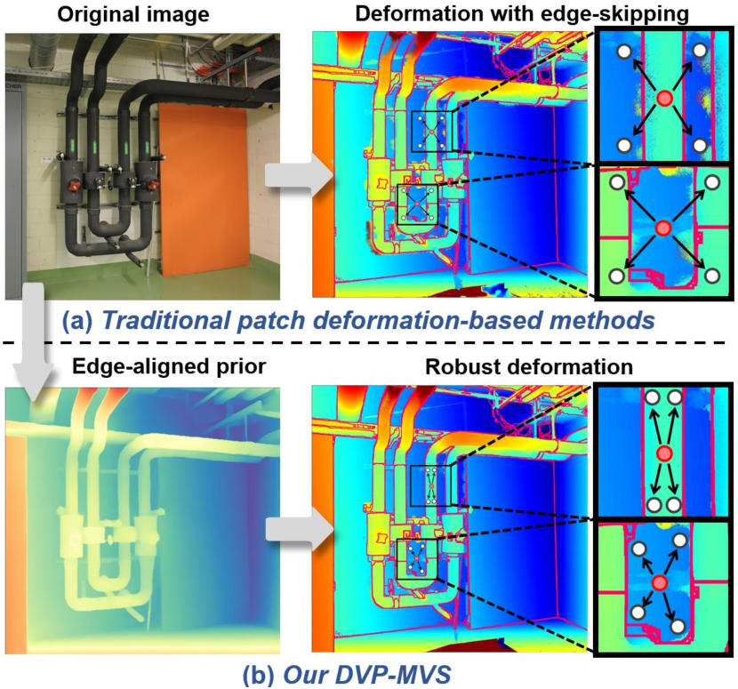
Figure 1: Comparison between patch deformation-based methods and ours. Edge-skipping causes other methods (a) incorrectly select reliable but depth-discontinuous gray pixels for patch deformation of the central unreliable red pixel. While our DVP-MVS (b) leverages depth-edge aligned prior to guarantee deformed patches within homogeneous areas.

To reconstruct textureless areas, two primary types of traditional MVS have been proposed: planarization-based and patch deformation-based methods. Planarization-based methods connect reliable pixels in well-textured areas to form regions that divide textureless areas, and then planarize these regions for reconstruction. Various strategies like superpixel (Yuan et al. 2024b), triangulation (Xu et al. 2022) and KD-tree (Ren et al. 2023) are employed, but these methods typically suffer from the limited size of connected regions and are prone to deviations during planarization.

Differently, patch deformation-based methods perform deformation on fixed patches to introduce enough features for matching costs. E.g., API-MVS (Sun et al. 2022) introduces entropy to increase the patch size and sampling intervals, while APD-MVS (Wang et al. 2023) adaptively searches for correlative reliable pixels around each unreliable pixel, then constructs multiple sub-patches centered on them for matching costs. However, such methods primarily concentrate on exploring advanced reliable pixel searching strategies to alleviate match ambiguity, but ignore a critical constraint for deformation stability (i.e., depth-edge aligned prior). As illustrated in Fig. 1(a), when reconstructing the unreliable red pixels (i.e., pixels with matching ambiguity), traditional patch deformation-based methods typically segment their surrounding areas into multiple fixed-angle sectors, and then search a reliable gray pixel within each sector to form patches. Nevertheless, during the process of searching for reliable pixels, unexpected edge-skipping caused by shadows or occlusions breaks the depth continuity principle, which may result in potential matching distortions.

Addressing this, we propose DVP-MVS, which innovatively synergizes depth-edge aligned and cross-view prior to facilitate robust and visibility-aware patch deformation. Specifically, we first utilize Depth Anything V2 (Yang et al. 2024) followed by the Roberts operator to initialize coarse depth and edge maps, respectively. The former maps provide monocular depth information for homogeneous areas (i.e., areas with depth continuity) in the global level, but lack detailed edge information. In contrast, the latter maps offer information about rough edges and dispersed regions. Consequently, we introduce an erosion-dilation strategy to align both types of maps for acquiring fine-grained homogeneous boundaries (i.e., bounds for homogeneous areas) to guide patch deformation, guaranteeing deformed patches within depth-continuous areas as shown in Fig. 1(b).

Furthermore, visibility occlusion is another crucial issue leading to unstable patch deformation. To mitigate this, we initially construct visibility maps by reforming view selection weights in ACMMP (Xu et al. 2022). Then, a post-verification algorithm based on coss-view depth reprojection is proposed for restoration of original-visible areas in visibility maps. Considering the restored visibility maps as the cross-view prior, we iteratively update deformed patches, thereby achieving visibility-aware patch deformation.

Finally, we improve the propagation and refinement process by integrating multi-view geometric consistency. Instead of randomly generating hypotheses as in previous methods, we aggregate visible hemispherical normals to constrain the normal ranges and adopt local projection depth differences on epipolar lines to limit the depth intervals. Evaluations on ETH3D and Tanks & Temples benchmarks demonstrate that our method can achieve state-of-the-art performance with excellent robustness and generalization.

In summary, our contributions are four-fold:

• For patch deformation-based MVS, we introduce depth-edge prior, which aligns coarse depth and edge information through an erosion-dilation strategy to generate fine-grained homogeneous boundaries for stable deformation.

• We construct visibility maps by reforming view selection weights and restoring visible areas with reprojection post-verification, which are then regarded as cross-view prior to facilitate visibility-aware patch deformation.

• Considering multi-view geometric consistency, we further improve the propagation and refinement process by introducing aggregated visible hemispherical normals and local projection depth differences on epipolar lines.

• We achieve the state-of-the-art performance on both the ETH3D and Tanks & Temples benchmarks.

Related Work

Traditional MVS Methods

PatchMatch MVS.

PatchMatch (Barnes et al. 2009) aims to search for the approximate patch pairs between two images. PatchMatchStereo (Bleyer, Rhemann, and Rother 2011) extends this idea to MVS, establishing the foundation for many subsequent methods. Gipuma (Galliani, Lasinger, and Schindler 2015) introduces a red-black checkerboard propagation to realize the parallelism of GPUs for acceleration. ACMM (Xu and Tao 2019) further proposes the adaptive checkerboard sampling and joint view selection to reconstruct textureless areas. To further reconstruct textureless areas, ACMMP (Xu et al. 2022) and HPM-MVS (Ren et al. 2023) respectively leverage triangulation and KD-tree to extract planes for planarization. Moreover, Pyramid (Liao et al. 2019) and MG-MVS (Wang et al. 2020) introduce hierarchical architecture to indirectly enhance the receptive field for reconstruction. MAR-MVS (Xu et al. 2020) introduces epipolar lines to analyze the geometry surface for optimal pixel level scale selection. Despite the significant improvements brought by these methods, the essential problem of insufficient patch receptive fields remains unresolved, leading to suboptimal reconstruction in textureless areas.

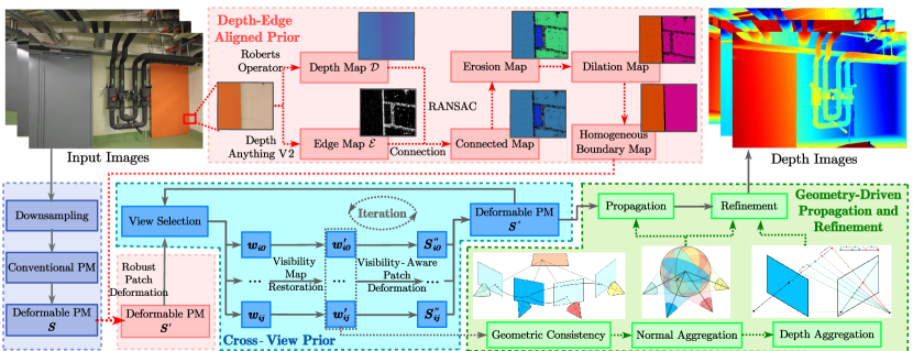
Figure 2: Pipeline of DVP-MVS. We first adopt Depth Anything V2 followed by the Roberts operator to initialize corresponding depth and edge maps, respectively. We then employ an erosion-dilation strategy to extract the depth-edge aligned prior for robust patch deformation. Subsequently, we construct visibility maps by reforming view selection and adopting the reprojection-based post-verification for visibility map restoration, which are then treated as the cross-view prior to facilitate visibility-aware patch deformation. Finally, by considering geometric consistency, we respectively improve the propagation and refinement stages by introducing visible normals aggregation and epipolar line projection. After several iterations we obtain depth images.

Patch Deformation.

As a branch of PatchMatch MVS, patch deformation adaptively expands patch receptive fields to help reconstruct textureless areas. Both patch resizing and patch reshaping belongs to patch deformation. For patch resizing, PHI-MVS (Sun et al. 2021) and API-MVS (Sun et al. 2022) respectively introduce dilated convolution and entropy calculation to modify patch size and sampling interval. However, an overlarge interval may cause sparse patch attention. For patch reshaping, SD-MVS (Yuan et al. 2024a) employs instance segmentation to constrain patch deformation within instances, while its results heavily depend on actual segmentation quality. Moreover, APD-MVS (Wang et al. 2023) separates the unreliable pixel’s patch into several outward-spreading sub-patches with high reliability. However, without depth edge constraint, deformed patches may occur edge-skipping to cover areas with depth-discontinuity.

Learning-based MVS Method

MVSNet (Yao et al. 2018) pioneers the use of convolutional neural networks to construct 3D differentiable cost volumes for reconstruction. R-MVSNet (Yao et al. 2019) and IterMVS-LS(Wang et al. 2022a) further incorporate the GRU module for regularization to facilitate the reconstruction of high-resolution scenarios. CVP-MVSNet (Yang et al. 2020a) and Cas-MVSNet (Yang et al. 2020b) leverage a coarse-to-fine strategy to achieve progressively refined depth estimation with less memory usage. Concerning epipolar lines, MVSTER (Wang et al. 2022b) proposes an epipolar transformer to learn both 2D semantics and 3D spatial associations. EPP-MVSNET (Ma et al. 2021) introduces an epipolar-assembling module to package images into limited cost volumes. GeoMVSNet (Zhang et al. 2023) integrates geometric priors from coarse stages through a two-branch fusion network to refine depth estimation progressively across finer stages. RA-MVSNet (Zhang, Zhu, and Lin 2023) utilizes a two-branch framework that integrates point-to-surface distance integration within cost volume to help reconstruct textureless area. ET-MVSNet (Liu et al. 2023) presents an epipolar transformer that constrains non-local feature aggregation within epipolar lines to aid in reconstruction. Despite this, most methods suffer from large training datasets, unaffordable memory usage or limited generalization. As such, we focus on traditional MVS.

Method

Overview

Given a series of input images $\mathcal{I}=\{I_{i}|i=1,...,N\}$ and their corresponding camera parameters $\mathcal{P}=\{K_{i},R_{i},T_{i}\mid i=1\cdots N\}$, we sequentially select the reference image $I_{\mathrm{ref}}$ from $\mathcal{I}$ and reconstruct its depth map through pairwise matching with the remaining source images $I_{\mathrm{src}}(\mathcal{I}-I_{\mathrm{ref}})$. Fig. 2 shows our method’s pipeline, and the implementation of each component will be detailed in the following sections.

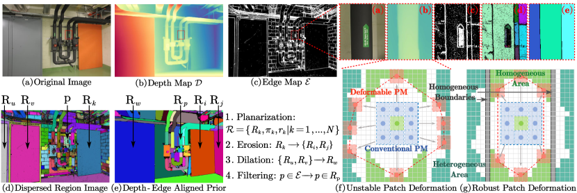
Figure 3: Depth-Edge Aligned Prior. Edges are highlighted in white in (c), with black constituting dispersed regions. Different colors denote different dispersed regions in (d) and homogeneous areas in (e), with black indicating their boundaries. In (f) and (g), green, blue and red respectively denote the central pixel, neighbors in conventional PM and anchors in deformable PM. Cyan, green and gray backgrounds respectively denote heterogeneous areas, homogeneous areas and homogeneous boundaries.

Preliminary Area

The conventional PM method projects a fixed-size patch in the reference image onto a corresponding patch in the source image with a given plane hypothesis. Subsequently, it calculates the similarity between the two patches using the NCC matrix (Schönberger et al. 2016) for evaluation. Specifically, given the reference image $I_{i}$ and the source image $I_{j}$, for each pixel $p$ in $I_{i}$, we first randomly generate a plane hypothesis $(\mathbf{n}^{T},d)$, where n and $d$ respectively denote the normal and the depth. Through homography mapping (Shen 2013), we can calculate the projection matrix $H_{ij}$ of the plane hypothesis $(\mathbf{n}^{T},d)$ for pixel $p$ between $I_{i}$ and $I_{j}$. We then employ $H_{ij}$ to project the fixed-size patch $B_{p}$ centered at $p$ in the reference image $I_{i}$ onto the mapping patch $B_{p}^{j}$ in the source image $I_{j}$. Consequently, the matching cost is calculated as the NCC score between $B_{p}$ and $B_{p}^{j}$, formulated by:

$$m_{ij}\left(p,B_{p}\right)=1-\frac{cov\left(B_{p},B_{p}^{j}\right)}{\sqrt{cov\left(B_{p},B_{p}\right)cov\left(B_{p}^{j},B_{p}^{j}\right)}},$$ (1)

where $cov$ is weighted covariance (Schönberger et al. 2016). Additionally, the multi-view aggregated cost is defined as:

$$m\left(p,B_{p}\right)=\frac{\sum^{N-1}_{j=1}w_{ij}(p)\cdot m_{ij}\left(p,B_{p}\right)}{\sum^{N-1}_{j=1}w_{ij}(p)},$$ (2)

where $w_{ij}(p)$ is gained from the view selection strategy (Xu et al. 2022). Finally, through propagation and refinement, we bring multiple hypotheses to each pixel for cost computation and select the minimal-cost hypothesis as the final result.

In contrast, the deformable PM (Wang et al. 2023) decomposes the patch of the unreliable pixel into several outward-spreading, reliable sub-patches, with the center of each sub-patch regarded as the anchor pixel. Specifically, for each unreliable pixel $p$, its matching cost of deformable PM is:

$$m_{ij}(p,S)=\lambda m_{ij}(p,B_{p})+(1-\lambda)\frac{\sum_{s\in S}m_{ij}(s,B_{s})}{|S|},$$ (3)

where $S$ denotes the collection of all anchors, $B_{s}$ represents the sub-patch with each anchor pixel $s\in S$ as center. In practice, the patch sizes of $B_{p}$ and $B_{s}$ are both $11\times 11$, while respective have sampling intervals 5 and 2. In experiment, $\lambda=0.25,|S|=8$.

Depth-Edge Aligned Prior

To reconstruct unreliable pixels in textureless areas, recent methods adopt patch deformation to expand the patch receptive field, while ignoring the critical depth edge constraint on deformation stability. As shown in Fig. 3 (f), the absence of depth edge constraint causes the deformed patch to occur edge-skipping and cover heterogeneous areas with depth discontinuity, leading to potential estimation deviation.

To fully exploit depth edges, we introduce the depth-edge aligned prior for robust patch deformation. Given image in Fig. 3 (a), we first utilize Depth Anything V2 (Yang et al. 2024) to initialize depth maps $\mathcal{D}$ in Fig. 3 (b). Depth Anything V2 is a robust monocular depth estimation model that can achieve zero-shot depth generalization across diverse scenarios. Meanwhile, we use Roberts operator on image $I$ to extract coarse edge maps $\mathcal{D}$ and dispersed regions $\mathcal{R}$ by connecting the remaining non-edge areas, represented with different colors in Fig. 3 (d). The whole process can be defined by: $I=\mathcal{D}\cup\mathcal{R}$. Moreover, we respectively define the heterogeneous region $H$, the homogeneous region $M$ and the homogeneous boundary $E$ as follows: $H=\{p\in\Omega\mid\nabla d_{p}>\epsilon\}$, $M=\{p\in\Omega\mid\nabla d_{p}\leq\epsilon\}$, $E_{i,j}=M_{i}\cap M_{j}$, where $\nabla d_{p}$ denotes depth gradient of pixel $p$, $\epsilon$ is set to 0.005. In addition, to align depth and edge maps for the generation of fine-grained homogeneous boundaries, a region-level erosion-dilation strategy is proposed to distinguish and aggregate homogeneous areas.

Specifically, given the dispersed region image shown in Fig. 3 (d), for each it dispersed region $R_{k}$ whose size exceeds $\eta$, we combine depth and region information from $\left[\mathcal{D},\mathcal{E}\right]$ to perform region-wise planarization with RANSAC, acquiring estimated plane $\pi_{k}=(n_{k},d_{k})$. Additionally, we define the ratio of inlier pixels to total pixels as the inlier ratio $r_{k}$. Therefore, we obtain $\mathcal{R}=\{R_{k},\pi_{k},r_{k}|k=1,...,N\}$. During the erosion stage, we perform intra-regional erosion to separate regions belonging to heterogeneous areas. For instance, region $R_{k}$ is pre-divided into sub-regions $R_{i}$ and $R_{j}$ by erosion. We then reapply planarization on both sub-regions to respectively acquire estimated planes $\pi_{i}=(n_{i},d_{i})$, $\pi_{j}=(n_{j},d_{j})$ and inlier ratio $r_{i}$, $r_{j}$. Ultimately, we consider erosion is effective and divide region $R_{k}$ when:

$$R_{k}\xrightarrow{}\left\{R_{i},R_{j}\right\}\text{, if }\text{sim}(\pi_{i},\pi_{j})\leq\sigma\text{ s.t. }\frac{r_{i}+r_{j}}{2r_{k}}\geq\gamma,$$ (4)

where plane similarity function $\text{sim}(\pi_{i},\pi_{j})$ is defined by:

$$\text{sim}(\pi_{i},\pi_{j})=\mathbf{n}_{i}\cdot\mathbf{n}_{j}+\min(1,|d_{i}-d_{j}|),$$ (5)

in Eq. 4, a higher inliers ratio indicates a superior planarization result after erosion, and a lower similarity in estimated planes indicates both sub-regions are located in homogeneous areas. On the contrary, for the dilation stage, we conduct inter-regional dilation to merge regions belonging to homogeneous areas. For example, regions $R_{u}$ and $R_{v}$ are pre-merged into an aggregated region $R_{w}$ through dilation. We then distinguish dilation is valid and perform region mergence under the following condition:

$$\{R_{u},R_{v}\}\xrightarrow{\text{}}R_{w}\text{, if }\text{sim}(\pi_{u},\pi_{v})\geq\sigma\text{ s.t. }r_{u},r_{v}\geq\kappa,$$ (6)

in Eq. 6, if two estimated planes are both reliable and similar to each other, we consider regions $R_{u}$ and $R_{v}$ should be merged together as homogeneous areas.

Following erosion-dilation strategy, we further incorporate pixel-wise filtering to refine fine-grained homogeneous boundaries. Specifically, when the pixel $p=(x,y,d_{p})$ with depth $d_{p}$ is adjacent to region $R_{p}$ with estimated plane $\pi_{k}=(\mathbf{n}_{k},d_{k})$, we regard $p$ belonging to $R_{p}$ provided that:

$$p\in\mathcal{E}\xrightarrow{\text{}}p\in R_{p}\text{, if }\frac{|\mathbf{n}_{k}\cdot p+d_{k}|}{|\mathbf{n}_{k}|}\leq\delta\text{ s.t. }r_{k}\geq\kappa,$$ (7)

in Eq. 7, if the 3D position of $p$ is close to the estimated plane, then $p$ should be considered as a part of region $R_{p}$. After obtaining the depth-edge aligned prior, we adopt it to guide patch deformation within homogeneous areas. Specifically, as shown in Fig. 3 (g), for unreliable pixel $p$, we first perform patch deformation to obtain the anchor collection $S$. Then for each anchor $s_{i}\in S$, we retain it if it lies in the same region as $p$; otherwise we discard it, formulated by:

$$S^{\prime}=\{s_{i}\in S\mid s_{i}\in R_{p}\},$$ (8)

where $S^{\prime}$ indicates the new anchor collection and $R_{p}$ signifies the homogeneous areas that $p$ belongs to. Finally, the new collection $S^{\prime}$ will substitute the old one $S$ for patch deformation, thereby avoiding unexpected edge-skipping and guaranteeing deformed patches within homogeneous areas.

Cross-View Prior

In addition to the aforementioned edge-skipping, the visibility discrepancy and occlusion caused by viewpoint changes is another crucial issue during patch deformation. As shown in Fig. 4, partial areas of the reference image in (a) may correspond to invisible areas in the source image in (b). However, the deformed patch in (e) frequently includes these invisible areas for matching cost, leading to potential distortions. Therefore, we attempt to progressively integrate cross-view prior to facilitate visibility-aware patch deformation.

Visibility Map Restoration.

For each pixel $p$ in the reference image $I_{i}$, we first initialize its visibility weights $w_{ij}(p)$ corresponding to source images $I_{j}$ through view selection strategy (Xu et al. 2022). Here $w_{ij}(p)$ is not simply used for cost aggregation but also reformulated as visibility maps to provide patch deformation with cross-view visibility perception. According to (Xu et al. 2022), $w_{ij}(p)$ is determined by evaluating costs against fixed thresholds. Therefore, low costs are more likely to be visible, while high costs are often deemed invisible. Thus, in textureless areas characterized by high costs, original-visible areas are often mistakenly judged as invisible, as shown in Fig.4 (c). Therefore, visibility determined merely by cost is unreliable, as it struggles to strike the balance between well-textured and textureless areas.

Essentially, visibility signifies the presence of corresponding pixel pairs between images, meaning each pixel can be mapped to the other via depth projection. Thus, we subtly adopt the cross-view depth reprojection $e(p)$ (Xu et al. 2022) as post-verification for visibility map restoration. Through back-and-forth projection, $e(p)$ can effectively validate the visibility between pixel pairs and the robustness of depths.

Specifically, for each pixel $p$ with depth $d$ in invisible areas of the reference image $I_{i}$, we first project it into source image $I_{j}$ to obtain pixel $p_{j}$. We then reproject $p_{j}$ with its corresponding depth $d_{j}$ in $I_{j}$ back into $I_{i}$ to derive reprojection pixel $p^{\prime}$. Ultimately, we define $e(p)=\left\|p^{\prime}-p\right\|$ and regard $p$ as visible with respect to $I_{j}$ when $e(p)\leq\varepsilon$, thereby generating restored weight $w_{ij}^{\prime}(p)$ and visibility map in Fig. 4 (d), which effectively restores the visibility in textureless areas.

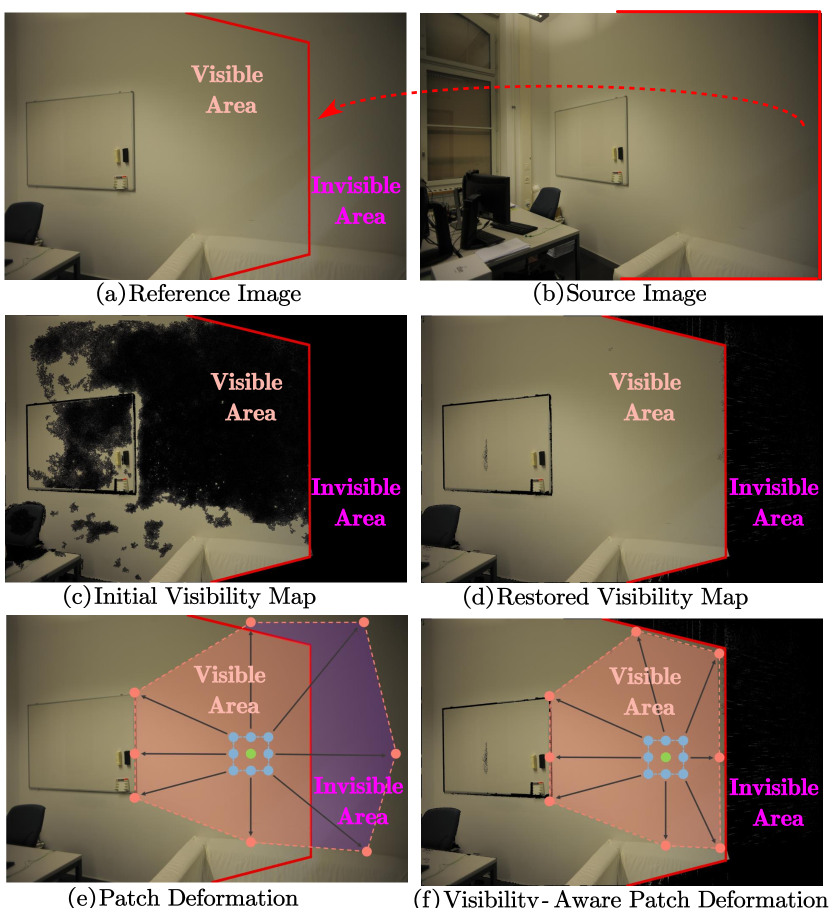
Figure 4: Cross-View Prior. The red line in (a) separates visible and invisible areas of (a) within (b). In (c) and (d), black indicates pixels judged invisible by view selection strategy. In (e) and (f), green, blue and red indicate the central pixel, conventional PM neighbors and deformable PM anchors.

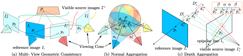
Figure 5: Geometry-Driven Propagation and Refinement. In (a) and (b), the blue view cone corresponds to the reference image $I_{i}$, while green, red, and yellow view cones correspond to visible source images $I^{v}_{0}$, $I^{v}_{1}$ and $I^{v}_{2}$.

Visibility-Aware Patch Deformation.

After acquiring the restored visibility map, we further regard it as cross-view prior to iteratively update patch deformation. Specifically, for each unreliable pixel $p$ in the reference image $I_{i}$, we first perform patch deformation to obtain anchor collection $S$, which is then guided by depth-edge prior to obtain $S^{\prime}$ via Eq. 8. Then for each anchor $s_{i}\in S^{\prime}$, we retain it if it is visible in source image $I_{j}$; otherwise, we discard it. Combined with Eq. 8, the view-level anchor collection $S_{ij}^{\prime}$ is defined by:

$$S_{ij}^{\prime\prime}=\{s_{i}\in S^{\prime}\mid s_{i}\in R_{p},w_{ij}(p)>0\}.$$ (9)

Subsequently, $S_{ij}^{\prime}$ will substitute $S$ in Eq. 3 to calculate the matching cost $m_{ij}(p,S_{ij}^{\prime})$, which in turn further optimizes $w_{ij}^{\prime}(p)$ during view selection, thereby iteratively facilitating visibility-aware patch deformation, as shown in Fig. 4 (f). Finally, the final multi-view aggregated cost $m(p,S^{\prime\prime})$ is:

$$m\left(p,S^{\prime\prime}\right)=\frac{\sum^{N-1}_{j=1}w_{ij}^{\prime}(p)\cdot m_{ij}\left(p,S_{ij}^{\prime\prime}\right)}{\sum^{N-1}_{j=1}w_{ij}^{\prime}(p)}.$$ (10)

Geometry-Driven Propagation and Refinement

Previous methods (Xu et al. 2022) incorporate neighborhood optimal hypotheses (i.e., normals and depths) for propagation and generate random hypotheses for refinement. However, the potential geometric constraint may render partial hypotheses invalid. Addressing this, we leverage the multi-view geometric consistency to improve propagation and refinement stages, including normal and depth aggregations.

Normal Aggregation.

To ensure geometric consistency, we first adopt the restored visibility maps to aggregate multi-view normals, thus restraining the normals in visible ranges. As shown in Fig. 5 (a), for each pixel $p_{i}$ in reference image $I_{i}$, we first leverage its restored visibility maps to identify all visible source images $\mathcal{I}^{v}=\{I^{v}_{j}|j=1,...,N-1,w_{ij}^{\prime}(p)>0\}$. We then utilize depth projection to obtain the 3D point $P$ and mapping pixels $p_{j}$ for each visible source image $I^{v}_{j}$. Since each $I^{v}_{j}$ in $\mathcal{I}^{v}$ has a visible hemisphere within its viewing cone and $P$ is visible to $I^{v}_{j}$, we can aggregate all visible hemispheres to constrain the normal range of 3D point $P$.

Specifically, we acquire the viewing cone direction $n^{v}_{j}$ of each visible source image $I^{v}_{j}$ by connecting its camera center with the mapping pixels $p_{j}$. Then, for each $I^{v}_{j}$, we consider the angle $\theta_{j}$ between its viewing cone direction $n^{v}_{j}$ and the normal $n_{P}$ of $P$ should exceed $90^{\circ}$ (i.e., $n_{P}\cdot n^{v}_{j}\leq 0$), as shown in Fig. 5 (b). Finally, by reprojecting the normal range of $P$ back to pixel $p_{i}$ in $I_{i}$, we effectively constrain the normal range of $n_{i}$. The aggregated normal range then serves as the visibility constraint during propagation and refinement, thereby enhancing the reliability of normal hypotheses.

Depth Aggregation.

For depth hypotheses, there exists two primary problems for conventional fixed depth intervals during the refinement process: $1)$ when depth interval is uniformly distributed in $I_{\mathrm{ref}}$ and projected onto $I_{\mathrm{src}}$, the spacing of the corresponding points along the epipolar line becomes uneven and progressively narrower as depth increases; $2)$ for each depth interval in $I_{\mathrm{ref}}$, the projected intervals along the epipolar lines can be variable in different source images.

Therefore, we perform inverse projection and aggregation of fixed-length sampling along multi-view epipolar lines to finetune the depth interval. Specifically, as illustrated in Fig. 5 (c), for each pixel $p_{i}$ in reference image $I_{i}$, we first identify its mapping pixel $p_{j}$ along epipolar line $l_{j}$ in visible source image $I^{v}_{j}$ as previously mentioned. We then select four pixels, located at distances $\alpha$ and $\alpha+\beta$ from $p$ on either side along epipolar line $l_{j}$, as the minimum and maximum disturbance extremes of mapping pixels. These four pixels are further inversely projected into the reference image $I_{i}$ to obtain their corresponding depths, thus forming two intervals for refinement: $D^{l}_{j}=(d^{ll}_{j},d^{lr}_{j})$ and $D^{r}_{j}=(d^{rl}_{j},d^{rr}_{j})$. Such adaptive intervals ensure that the mapping pixel of refined hypothesis can achieve appropriate displacements along the epipolar line without being constrained by the current depth.

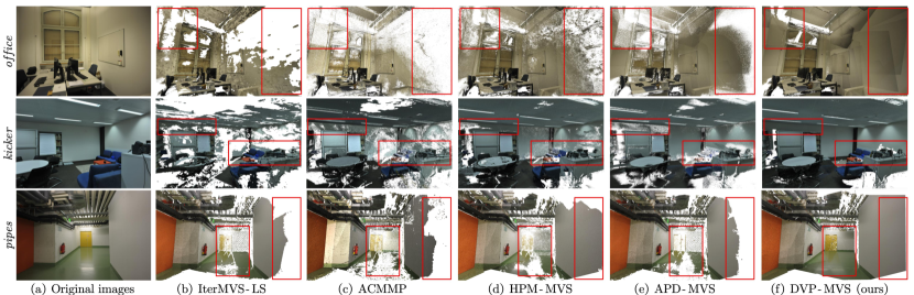
Figure 6: Qualitative results on partial scenes of ETH3D datasets (office, kicker and pipes). Our method can achieve the highest completeness while containing fewer outliers, especially in large textureless areas like walls and floors, as shown in red boxes.

Moreover, to ensure mapping pixels experiences notably displacements in as many source images as possible, we aggregate depth intervals across all visible source images $\mathcal{I}^{v}$. Specifically, we identify the extremes of aggregated intervals as the $\mu^{th}$ smallest value among all maximum disturbance extremes (i.e., $d^{ll}_{j}$ and $d^{rr}_{j}$) and the $\mu^{th}$ largest value among all minimum disturbance extremes (i.e., $d^{lr}_{j}$ and $d^{rl}_{j}$):

$$\left(\min_{1\leq j\leq\mu}d^{ll}_{j},\max_{1\leq j\leq\mu}d^{lr}_{j}\right),\left(\max_{1\leq j\leq\mu}d^{rl}_{j},\min_{1\leq j\leq\mu}d^{rr}_{j}\right).$$ (11)

A detailed explanation of this equation is shown in supplementary material. Finally, the aggregated depth interval will replace the fixed depth interval during local perturbations of refinement to enhance the reliability of depth hypotheses.

Experiment

Datasets, Metrics and Implementation Details

We evaluate our work on both ETH3D (Schops et al. 2017) and Tanks & Temples (TNT) (Knapitsch et al. 2017) datasets and upload our results to their websites for reference. We compare our work against state-of-the-art learning-based methods like PatchMatchNet, IterMVS, MVSTER, AA-RMVSNet, EPP-MVSNet, EPNet and state-of-the-art traditional MVS methods like TAPA-MVS, PCF-MVS, ACMM, ACMP, ACMMP, SD-MVS, APD-MVS and HPM-MVS.

Concerning metrics, we adopt the percentage of accuracy and completeness for evaluation, with the F₁ score adopted as their harmonic mean to measure the overall quality.

We take APD-MVS (Wang et al. 2023) as our baseline. Concerning parameter setting, $\{\eta,\sigma,\gamma,\kappa,\delta,\varepsilon,\alpha,\beta,\mu\}=\{3\times 10^{2},0.5,1.2,0.7,0.8,2,1,4,3\}$.

Our method is implemented on a machine with an Intel(R) Xeon(R) Silver 4210 CPU and eight NVIDIA GeForce RTX 3090 GPUs. We take APD-MVS (Wang et al. 2023) as our baseline. Experiments are performed on original images in both ETH3D and TNT datasets. In cost calculation, we adopt the matching strategy of every other row and column.

Method	Train			Test
	F1	Comp.	Acc.	F1	Comp.	Acc.
PatchMatchNet	64.21	65.43	64.81	73.12	77.46	69.71
IterMVS-LS	71.69	66.08	79.79	80.06	76.49	84.73
MVSTER	72.06	76.92	68.08	79.01	82.47	77.09
EPP-MVSNet	74.00	67.58	82.76	83.40	81.79	85.47
EPNet	79.08	79.28	79.36	83.72	87.84	80.37
TAPA-MVS	77.69	71.45	85.88	79.15	74.94	85.71
PCF-MVS	79.42	75.73	84.11	80.38	79.29	82.15
ACMM	78.86	70.42	90.67	80.78	74.34	90.65
ACMMP	83.42	77.61	90.63	85.89	81.49	91.91
SD-MVS	86.94	84.52	89.63	88.06	87.49	88.96
HPM-MVS++	87.09	85.64	88.74	89.02	89.37	88.93
APD-MVS (base)	86.84	84.83	89.14	87.44	85.93	89.54
DVP-MVS (ours)	88.67	88.07	89.40	89.60	89.41	91.32

Table 1: Quantitative results on ETH3D dataset at threshold $2cm$. Our method achieves the highest F₁ and completeness.

Benchmark Performance

Regarding ETH3D dataset, Fig. 6 shows the qualitative comparison. Our method can reconstruct textureless areas without detail distortion, as shown in red boxes. Tab. 1 exhibits the quantitative analysis, where the first group is learning-based methods and the second is traditional methods. Meanwhile, the best and the second-best results are respectively marked in bold and underlined. Our method achieves the highest F₁ scores and completeness on both training and testing datasets, validating its excellent effectiveness.

Regarding TNT dataset, we test our method on it without fine-tuning to prove generalization. Tab. 2 exhibits the quantitative analysis. Our method achieves the highest completeness on both advanced and intermediate datasets and the highest F₁ scores on intermediate dataset, demonstrating its astonishing robustness. More qualitative results on both ETH3D and TNT datasets along with a detailed memory and runtime comparison are shown in supplementary materials.

Method	Intermediate			Advanced
	F1	Rec.	Pre.	F1	Rec.	Pre.
PatchMatchNet	53.15	69.37	43.64	32.31	41.66	27.27
AA-RMVSNet	61.51	75.69	52.68	33.53	33.01	37.46
IterMVS-LS	56.94	74.69	47.53	34.17	44.19	28.70
MVSTER	60.92	77.50	50.17	37.53	45.90	33.23
EPP-MVSNet	61.68	75.58	53.09	35.72	34.63	40.09
EPNet	63.68	72.57	57.01	40.52	50.54	34.26
ACMM	57.27	70.85	49.19	34.02	34.90	35.63
ACMP	58.41	73.85	49.06	37.44	42.48	34.57
ACMMP	59.38	68.50	53.28	37.84	44.64	33.79
SD-MVS	63.31	76.63	53.78	40.18	47.37	35.53
HPM-MVS++	61.59	73.79	54.01	39.65	41.09	40.79
APD-MVS (base)	63.64	75.06	55.58	39.91	49.41	33.77
DVP-MVS (ours)	64.76	78.69	55.04	40.23	54.21	32.16

Table 2: Quantitative results on TNT dataset at given threshold. Our method achieves the highest F₁ and completeness.

Memory & Runtime Comparison

To validate the efficiency of our proposed method, we perform a comparative analysis of GPU memory usage and runtime of different methods on the ETH3D training datasets, as depicted in Fig. 7. All experiments were conducted on original-resolution images, with the number of images standardized to 10 for consistency in the runtime evaluation. Furthermore, to ensure fairness, all methods were evaluated on the same hardware, whose configuration has been detailed in the previous section. The F₁ scores of each method at threshold $2cm$ on the ETH3D training dataset are indicated next to the corresponding pattern for comparsion.

Regarding learning-based MVS methods, IterMVS-LS achieves the shortest runtime but exhibits excessive memory consumption, exceeding the limitations of mainstream GPUs. Other learning-based MVS methods also encounter similar memory-related limitations, thus restricting their applicability for large-scale scenario reconstructions.

Concerning traditional MVS methods, although ACMM, ACMP, and ACMMP achieve relatively shorter runtimes with comparable memory usage, our method delivers significantly better results. Compared to baseline APD-MVS, our method consumes similar runtime and memory usage while achieving superior performance. Additionally, our method comprehensively outclasses HPM-MVS in terms of runtime, memory and reconstruction quality. In summary, our method can deliver SOTA performance with acceptable runtime and memory usage, demonstrating its considerable practicality.

Method	$2cm$			$10cm$
	F1	Comp.	Acc.	F1	Comp.	Acc.
w/o. Agn.	86.53	84.43	88.85	96.46	95.10	97.89
w/o. Ero.	88.02	86.95	89.23	97.52	96.89	98.15
w/o. Dil.	87.56	86.19	89.03	97.14	96.28	98.01
w/o. Fil.	87.75	86.52	89.12	97.28	96.51	98.07
w/o. Cro.	86.76	84.92	88.79	96.61	95.43	97.85
w/o. Res.	87.84	86.67	89.15	97.35	96.64	98.10
w/o. Vis.	87.39	86.09	88.86	97.05	96.27	97.87
w/o. Geo.	86.92	85.39	88.63	96.73	95.76	97.74
w/o. Pro.	88.13	87.25	89.16	97.54	96.99	98.08
w/o. Ref.	87.69	86.58	88.96	97.25	96.55	97.96
w/o. Dep.	87.62	86.36	89.04	97.21	96.42	98.01
DVP-MVS	88.67	88.07	89.40	97.93	97.61	98.27

Table 3: Quantitative results of the ablation studies on ETH3D benchmark to validate each proposed component.

Ablation Study

Tab. 3 exhibits detailed ablation studies on ETH3D dataset.

Depth-Edge Aligned Prior

We separately exclude the whole depth-edge aligned prior (w/o. Agn.), region erosion (w/o. Ero.), region dilation (w/o. Dil.), and pixel-wise filtering (w/o. Fil.). Obviously, w/o. Agn. produces the worst F₁ score, highlighting the significance of edge constraint for patch deformation. The F₁ score of w/o. Ero. is slightly better than w/o. Dil., meaning region dilation exhibits greater impacts than region erosion. Moreover, both w/o. Dil. and w/o. Fil. delivere similar F₁ score, yet fell short when compared with DVP-MVS, indicating that region erosion and pixel-wise filtering are equally crucial.

Cross-View Prior

We individually remove the entire cross-view prior (w/o. Cro.), visibility map restoration (w/o. Res.), and visibility-aware patch deformation (w/o. Vis.). In comparison, w/o. Cro. yields the lowest F₁ score, validating the importance of cross-view prior for visibility-aware patch deformation. Moreover, w/o. Res. attains a higher F₁ score than w/o. Vis., emphasizing visibility-aware patch deformation is more crucial than visibility map restoration.

Geometry-Driven Propagation and Refinement

We respectively remove the whole geometry-driven module (w/o. Geo.), normal constraint for propagation (w/o. Pro.) and refinement (w/o. Ref.), and depth constrains for refinement (w/o. Dep.). Evidently, without geometric constraint, w/o. Geo. obtains the worst F₁ score. The F₁ score of w/o. Pro. surpasses w/o. Ref., suggesting that the normal constraint is more beneficial to refinement than propagation. Moreover, the similar F₁ score of w/o. Ref. and w/o. Dep. indicates that normal and depth constraints are equivalently contributive.

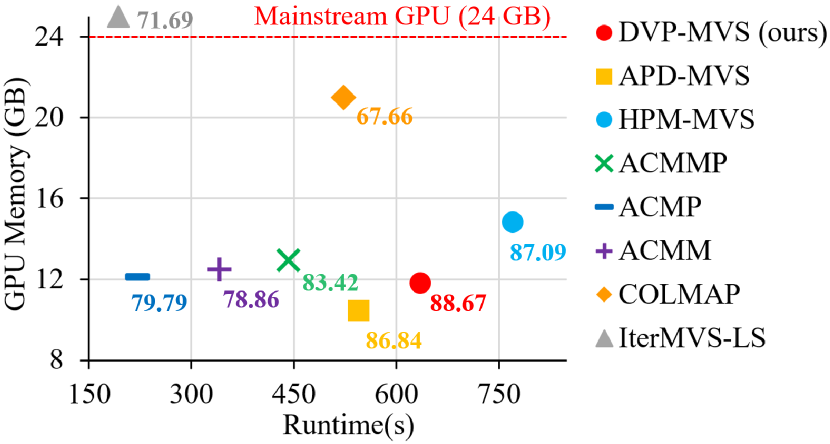
Figure 7: GPU memory usage (GB) and runtime (second) between different methods on ETH3D training datasets.

Conclusion

In this paper, we propose DVP-MVS to synergize depth-edge aligned and cross-view prior for robust and visibility-aware patch deformation. For robust patch deformation, depth and edge information are aligned with an erosion-dilation strategy to guarantee deformed patches within homogeneous areas. For visibility-aware patch deformation, we reform and restore visibility maps and regard them as cross-view prior to bring deformed patches visibility perception. Additionally, we incorporate multi-view geometric consistency to improve propagation and refinement with reliable hypotheses. Experimental results on ETH3D and TNT datasets indicate our method’s state-of-the-art performance.

References

- Barnes et al. (2009) Barnes, C.; Shechtman, E.; Finkelstein, A.; and Goldman, D. B. 2009. PatchMatch: A randomized correspondence algorithm for structural image editing. ACM Trans. Graph., 28(3): 24.
- Bleyer, Rhemann, and Rother (2011) Bleyer, M.; Rhemann, C.; and Rother, C. 2011. PatchMatch Stereo - Stereo Matching with Slanted Support Windows. In Hoey, J.; McKenna, S. J.; and Trucco, E., eds., British Mach. Vis. Conf. (BMVC), 1–11.
- Galliani, Lasinger, and Schindler (2015) Galliani, S.; Lasinger, K.; and Schindler, K. 2015. Massively Parallel Multiview Stereopsis by Surface Normal Diffusion. In Proc. IEEE/CVF Int. Conf. Comput. Vis. (ICCV).
- Knapitsch et al. (2017) Knapitsch, A.; Park, J.; Zhou, Q.-Y.; and Koltun, V. 2017. Tanks and Temples: Benchmarking Large-Scale Scene Reconstruction. ACM Transactions on Graphics (ToG), 36(4): 1–13.
- Liao et al. (2019) Liao, J.; Fu, Y.; Yan, Q.; and Xiao, C. 2019. Pyramid Multi-View Stereo with Local Consistency. Computer Graphics Forum, 38(7): 335–346.
- Liu et al. (2023) Liu, T.; Ye, X.; Zhao, W.; Pan, Z.; Shi, M.; and Cao, Z. 2023. When Epipolar Constraint Meets Non-Local Operators in Multi-View Stereo. In Proceedings of the IEEE/CVF International Conference on Computer Vision, 18088–18097.
- Lu et al. (2024) Lu, H.; Tang, J.; Xu, X.; Cao, X.; Zhang, Y.; Wang, G.; Du, D.; Chen, H.; and Chen, Y. 2024. Scaling Multi-Camera 3D Object Detection through Weak-to-Strong Eliciting. arXiv:2404.06700.
- Ma et al. (2021) Ma, X.; Gong, Y.; Wang, Q.; Huang, J.; Chen, L.; and Yu, F. 2021. Epp-Mvsnet: Epipolar-assembling Based Depth Prediction for Multi-View Stereo. In Proceedings of the IEEE/CVF International Conference on Computer Vision, 5732–5740.
- Ren et al. (2023) Ren, C.; Xu, Q.; Zhang, S.; and Yang, J. 2023. Hierarchical Prior Mining for Non-Local Multi-View Stereo. In Proceedings of the IEEE/CVF International Conference on Computer Vision, 3611–3620.
- Schönberger et al. (2016) Schönberger, J. L.; Zheng, E.; Frahm, J.-M.; and Pollefeys, M. 2016. Pixelwise View Selection for Unstructured Multi-View Stereo. In Proc. Eur. Conf. Comput. Vis. (ECCV), 501–518.
- Schops et al. (2017) Schops, T.; Schonberger, J. L.; Galliani, S.; Sattler, T.; Schindler, K.; Pollefeys, M.; and Geiger, A. 2017. A Multi-View Stereo Benchmark With High-Resolution Images and Multi-Camera Videos. In Proc. IEEE/CVF Conf. Comput. Vis. Pattern Recognit. (CVPR).
- Shen (2013) Shen, S. 2013. Accurate Multiple View 3D Reconstruction Using Patch-Based Stereo for Large-Scale Scenes. IEEE Trans. Image Process., 22(5): 1901–1914.
- Sun et al. (2022) Sun, S.; Liu, J.; Li, Y.; Ying, H.; Zhai, Z.; and Mou, Y. 2022. Adaptive Pixelwise Inference Multi-View Stereo. In Xu, D.; and Xiao, L., eds., Thirteenth International Conference on Graphics and Image Processing (ICGIP 2021), 77. Kunming, China: SPIE. ISBN 978-1-5106-5042-8 978-1-5106-5043-5.
- Sun et al. (2021) Sun, S.; Zheng, Y.; Shi, X.; Xu, Z.; and Liu, Y. 2021. Phi-Mvs: Plane Hypothesis Inference Multi-View Stereo for Large-Scale Scene Reconstruction. arXiv preprint arXiv:2104.06165.
- Tan et al. (2023) Tan, R.; Wang, Q.; Wang, X.; Yan, C.; Sun, Y.; and Feng, Y. 2023. MP-MVS: Multi-Scale Windows PatchMatch and Planar Prior Multi-View Stereo. arXiv:2309.13294.
- Wang et al. (2022a) Wang, F.; Galliani, S.; Vogel, C.; and Pollefeys, M. 2022a. IterMVS: Iterative probability estimation for efficient multi-view stereo. In Proc. IEEE/CVF Conf. Comput. Vis. Pattern Recognit. (CVPR), 8606–8615.
- Wang et al. (2024) Wang, J.; Ivrissimtzis, I.; Li, Z.; and Shi, L. 2024. Comparative Efficacy of 2D and 3D Virtual Reality Games in American Sign Language Learning. In 2024 IEEE Conference on Virtual Reality and 3D User Interfaces Abstracts and Workshops (VRW), 875–876. IEEE.
- Wang et al. (2022b) Wang, X.; Zhu, Z.; Huang, G.; Qin, F.; Ye, Y.; He, Y.; Chi, X.; and Wang, X. 2022b. MVSTER: Epipolar Transformer for Efficient Multi-View Stereo. In European Conference on Computer Vision, 573–591. Springer.
- Wang et al. (2020) Wang, Y.; Guan, T.; Chen, Z.; Luo, Y.; Luo, K.; and Ju, L. 2020. Mesh-Guided Multi-View Stereo With Pyramid Architecture. In Proc. IEEE/CVF Conf. Comput. Vis. Pattern Recognit. (CVPR), 2036–2045.
- Wang et al. (2023) Wang, Y.; Zeng, Z.; Guan, T.; Yang, W.; Chen, Z.; Liu, W.; Xu, L.; and Luo, Y. 2023. Adaptive Patch Deformation for Textureless-Resilient Multi-View Stereo. In Proc. IEEE/CVF Conf. Comput. Vis. Pattern Recognit. (CVPR), 1621–1630.
- Wei et al. (2023) Wei, Y.; Zhao, L.; Zheng, W.; Zhu, Z.; Zhou, J.; and Lu, J. 2023. Surroundocc: Multi-camera 3d Occupancy Prediction for Autonomous Driving. In Proceedings of the IEEE/CVF International Conference on Computer Vision, 21729–21740.
- Wu et al. (2024) Wu, J.; Li, R.; Xu, H.; Zhao, W.; Zhu, Y.; Sun, J.; and Zhang, Y. 2024. GoMVS: Geometrically Consistent Cost Aggregation for Multi-View Stereo. In Proceedings of the IEEE/CVF Conference on Computer Vision and Pattern Recognition, 20207–20216.
- Xu et al. (2022) Xu, Q.; Kong, W.; Tao, W.; and Pollefeys, M. 2022. Multi-Scale Geometric Consistency Guided and Planar Prior Assisted Multi-View Stereo. IEEE Transactions on Pattern Analysis and Machine Intelligence.
- Xu and Tao (2019) Xu, Q.; and Tao, W. 2019. Multi-Scale Geometric Consistency Guided Multi-View Stereo. In Proc. IEEE/CVF Conf. Comput. Vis. Pattern Recognit. (CVPR).
- Xu et al. (2020) Xu, Z.; Liu, Y.; Shi, X.; Wang, Y.; and Zheng, Y. 2020. MARMVS: Matching Ambiguity Reduced Multiple View Stereo for Efficient Large Scale Scene Reconstruction. In Proc. IEEE/CVF Conf. Comput. Vis. Pattern Recognit. (CVPR), 5980–5989.
- Yang et al. (2020a) Yang, J.; Mao, W.; Alvarez, J. M.; and Liu, M. 2020a. Cost Volume Pyramid Based Depth Inference for Multi-View Stereo. In Proceedings of the IEEE/CVF Conference on Computer Vision and Pattern Recognition, 4877–4886.
- Yang et al. (2020b) Yang, J.; Mao, W.; Alvarez, J. M.; and Liu, M. 2020b. Cost Volume Pyramid Based Depth Inference for Multi-View Stereo. In Proc. IEEE/CVF Conf. Comput. Vis. Pattern Recognit. (CVPR), 4876–4885.
- Yang et al. (2024) Yang, L.; Kang, B.; Huang, Z.; Zhao, Z.; Xu, X.; Feng, J.; and Zhao, H. 2024. Depth Anything V2. arXiv:2406.09414.
- Yao et al. (2018) Yao, Y.; Luo, Z.; Li, S.; Fang, T.; and Quan, L. 2018. MVSNet: Depth Inference for Unstructured Multi-view Stereo. In Proc. Eur. Conf. Comput. Vis. (ECCV).
- Yao et al. (2019) Yao, Y.; Luo, Z.; Li, S.; Shen, T.; Fang, T.; and Quan, L. 2019. Recurrent Mvsnet for High-Resolution Multi-View Stereo Depth Inference. In Proceedings of the IEEE/CVF Conference on Computer Vision and Pattern Recognition, 5525–5534.
- Yao et al. (2020) Yao, Y.; Luo, Z.; Li, S.; Zhang, J.; Ren, Y.; Zhou, L.; Fang, T.; and Quan, L. 2020. Blendedmvs: A Large-Scale Dataset for Generalized Multi-View Stereo Networks. In Proceedings of the IEEE/CVF Conference on Computer Vision and Pattern Recognition, 1790–1799.
- Yuan et al. (2024a) Yuan, Z.; Cao, J.; Li, Z.; Jiang, H.; and Wang, Z. 2024a. SD-MVS: Segmentation-driven Deformation Multi-View Stereo with Spherical Refinement and EM Optimization. Proceedings of the AAAI Conference on Artificial Intelligence, 38(7): 6871–6880.
- Yuan et al. (2024b) Yuan, Z.; Cao, J.; Wang, Z.; and Li, Z. 2024b. Tsar-Mvs: Textureless-aware Segmentation and Correlative Refinement Guided Multi-View Stereo. Pattern Recognition, 110565.
- Zhang, Zhu, and Lin (2023) Zhang, Y.; Zhu, J.; and Lin, L. 2023. Multi-View Stereo Representation Revist: Region-Aware MVSNet. In Proceedings of the IEEE/CVF Conference on Computer Vision and Pattern Recognition, 17376–17385.
- Zhang et al. (2023) Zhang, Z.; Peng, R.; Hu, Y.; and Wang, R. 2023. GeoMVSNet: Learning Multi-View Stereo With Geometry Perception. In Proceedings of the IEEE/CVF Conference on Computer Vision and Pattern Recognition, 21508–21518.