Aligning Visual and Semantic Interpretability through Visually Grounded Concept Bottleneck Models

Abstract

The performance of neural networks increases steadily, but our understanding of their decision-making lags behind. Concept Bottleneck Models (CBMs) address this issue by incorporating human-understandable concepts into the prediction process, thereby enhancing transparency and interpretability. Since existing approaches often rely on large language models (LLMs) to infer concepts, their results may contain inaccurate or incomplete mappings, especially in complex visual domains. We introduce visually Grounded Concept Bottleneck Models (GCBM), which derive concepts on the image level using segmentation and detection foundation models. Our method generates inherently interpretable concepts, which can be grounded in the input image using attribution methods, allowing interpretations to be traced back to the image plane. We show that GCBM concepts are meaningful interpretability vehicles, which aid our understanding of model embedding spaces. GCBMs allow users to control the granularity, number, and naming of concepts, providing flexibility and are easily adaptable to new datasets without pre-training or additional data needed. Prediction accuracy is within 0.3-6% of the linear probe and GCBMs perform especially well for fine-grained classification interpretability on CUB, due to their dataset specificity. Our code is available on https://github.com/KathPra/GCBM.

1 Introduction

The success of deep neural networks (DNNs) has led to their widespread application in various tasks, from everyday interactions like voice assistants to complex domains such as medical image analysis with the goal of generating treatment recommendations. Despite their capabilities, the opaque nature of DNNs presents significant challenges in terms of reliability, especially in safety-critical systems, where a lack of interpretability can limit their adaptation. Explainable Artificial Intelligence (XAI) is a field that addresses these issues by making “black-box” models’ decisions more transparent and interpretable.

Concept Bottleneck Models (CBMs) [1] offer an inherently interpretable approach by classifying based on a linear combination of semantic concepts. The interpretability of classification decisions depends on the quality of the concept-level representations. Therefore, it is crucial to derive concepts that are both understandable to humans and intuitively consistent with the internal semantics of the model. While early CBM works have many annotated concepts, it has recently become popular to use an LLM to generate the concept set [2, 3, 4]. However, this carries the risk of integrating LLM bias into the concept set. In line with parallel work [5, 6] we advocate for LLM-free approaches.

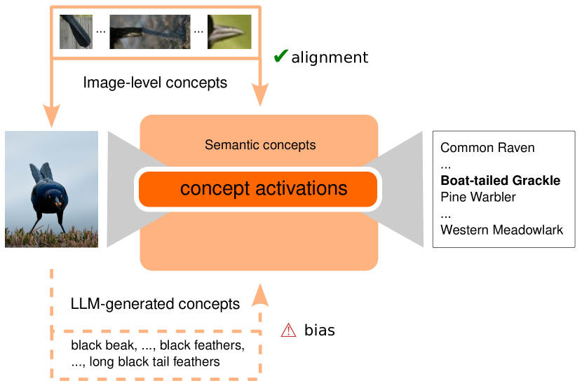
Figure 1: GCBMs are visually aligned CBMs. Finding concepts is the key challenge in CBMs as they are decisive for the model interpretability. GCBMs create visual and semantic aligned concepts, which allow end-to-end interpretability. In contrast, LLM-based concept generation approaches risk biases in the concept set.

With Visually Grounded Concept Bottleneck Models (GCBMs), we propose a simple and efficient framework, that leverages recent advances in segmentation and detection foundation models to extract training image regions as concepts, ranging from coarse to fine-grained. Figure 1 highlights the key distinctions and motivation between GCBM and LLM-based CBMs, which work well even in specialized domains. GCBMs offer a flexible adaptation of novel datasets; it can provide dataset-specific interpretability without requiring pre-training. This sets us apart from other LLM-free approaches which either use general pre-training [5] or pre-trained embedding models [6]. To the best of our knowledge, we are the first to use image-level concepts for CBMs. By grounding concepts visually, we enable a more direct and intuitive understanding of the model’s decision-making process, allowing for the examination of key image concepts utilized by the CBM in its predictions. We frame GCBMs as the intersection of CBMs [7, 3, 5, 8, 9, 10, 6, 11, 12, 13, 14, 15], part-based classifiers [16, 17, 18, 19, 20, 21], and attribution methods [22, 23].

The main contributions of this work are as follows:

• With GCBMs, we introduce a simple and efficient framework that can easily be adapted to novel datasets as it requires neither pretraining nor a pre-defined concept set.

• We create image-level concepts using segmentation and detection models, which are visually and semantically aligned. To minimize potential hallucinations and bias, we do not integrate LLMs in their concept generation.

• We extensively evaluate our framework across concept proposal generation methods and datasets and discuss its interpretability on several examples.

• Evaluating on ImageNet-R, we show that concepts from our GCBMs are robust to changes in image domain. To the best of our knowledge, we are the first to evaluate the generalization of these concepts.

2 Related work

Explainable artificial intelligence aims to make model decisions comprehensible. Post-hoc methods, which generate an explanation after the model prediction, provide insights in the image area relevant for the model decisions e.g. [24, 25, 22]. Their interpretability is limited, as they answer the what and not the why of model decisions [26, 27]. Ante-hoc methods are inherently interpretable and provide the prediction along with its explanation e.g. [5, 2, 7, 3, 28]. They include single linear neural networks, decision trees, and self-explaining networks e.g. DEAL [29], BCOS-networks [30], and LLaVA [31]. Using LLMs and VLMs induces the risk of hallucinations in model explanations [32].

Concept bottleneck models predict image classes based on linear combinations of concepts. We compare GCBMs to CBMs as we use the same pipeline of concept generation and linear probing. CBMs mainly differ in the way they extract the concepts. Menon and Vondrick [2] generate GPT-3 descriptions of class-specific concepts, providing insights into the visual attributes associated with each category (DCLIP). Similarly, Oikarinen et al. [3] generate concept sets for CBMs using also GPT-3 for their model called label-free CBM (LF-CBM). They employ CLIP-Dissect [4], which constructs a concept matrix based on textual embeddings from the LLM and corresponding input images and optimizes their alignment. Panousis et al. [8] extend LF-CBM by incorporating a sparse concept discovery module (CDM) that encourages sparsity and is modeled with a Bernoulli distribution. Language-guided CBM (LaBo) employs GPT-3 for concept creation, but it stands out by using a submodular function to select concepts from candidate sets, building the bottleneck, and training a linear model based on CLIP embeddings Yang et al. [7]. Rao et al. [5] introduce the Discover-then-Name (DN-CBM), which employs sparse autoencoders for concept generation. These concepts are then mapped to names derived from a corpus of broad textual descriptions, and the resulting mapped concepts are used to train a CBM. Parallel work by Schrodi et al. [6] understands concepts as low-rank approximations of model activations, which they learn using non-negative matrix factorization. In line with these works, we argue that concept extraction should not be pre-defined, neither in terms of the number of concepts nor in the type of concepts.

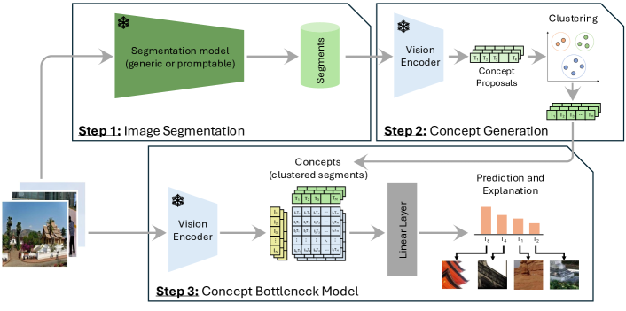
Figure 2: GCBM framework. The GCBM framework begins by generating concept proposals through segmentation models (Step 1). These proposals are then clustered, each represented by its centroid (Step 2). Finally, the unique concepts are utilized to train a sparse CBM, effectively grounding the concepts in the input image (Step 3).

CBM concept generation typically contains autoencoders [5, 10], non-negative matrix factorization [6, 11, 12], K-Means [13], or PCA [14, 11]. Panousis et al. [9] share our conviction, that multi-level concepts enhance the expressiveness of CBMs. In contrast to their 2-level approach, our GCBM can detect multi-level concepts. We generate GCBM concept proposals in an unsupervised manner using existing segmentation [33, 34, 35, 36, 37] and detection models [38]. Promptable detection methods are steered more than generic models and produce more part-like concepts. This way, we can extract multiple concept proposals per image and can process any type of image. The numerous concept proposals generated through this process are consolidated into distinct concepts using clustering. We name our generated concepts, as proposed by [5], using the CLIP embedding space and common concept and attribute sets. Kowal et al. [39] also employ segmentation for interpretability, however, their work focuses on matching concept representations from different layers of the network and not like GCBM on finding representative concepts for interpretable model predictions.

Part-based classifiers [16, 17, 19, 20, 21, 18] base their class predictions on image parts, instead of the whole image. Conceptually, they are based on Bags of Visual Words [40]. Modern part-based models are trained end-to-end, learning optimized prototypes for a given task. Chen et al. [19] learns 10 prototypes per class and visualizes them in the input image using CAM [41]. [16] use a CLIP-based detector to identify pre-defined image parts. Similarly, in GCBMs, we break down the image into individual parts to increase interpretability. However, we do not influence the number of parts per image and allow shared parts between classes, by first selecting a large number of proposals which we then reduce to concepts using clustering.

Attribution methods [23, 22, 25, 24] trace model decisions back to the image area on which the model is basing them. They determine the relevant image region by using e.g. gradients, activations, occlusions or perturbations. Grad-CAM [22], for instance, visualizes the activations of the network’s final layer, while Local Interpretable Model-agnostic Explanations (LIME) [24, 25] uses perturbation-based surrogates to approximate interpretable models. For GCBM, we employ GradCAM to anchor the derived concepts in the input image, leveraging its model-specific properties.

3 Visually grounded concept bottleneck models (GCBMs)

The GCBM approach grounds image concepts by anchoring them to specific image segments, enabling the training of a standard CBM that effectively associates relevant concepts with corresponding regions in the input image. Figure 2 illustrates the GCBM framework that derives visual and semantic aligned concepts.

3.1 Concept proposal generation

We create a concept proposal image subset $\mathcal{D}$, for which we segment 50 training images per dataset class. We utilize this subset of the training dataset not only to help mitigate the risk of overfitting but also to ensure the model is tailored to the specific characteristics of the dataset. The number of training samples can be further reduced to save computational resources as reported in Sec. D.1. Each image $i$ in $\mathcal{D}$ is segmented into $l_{i}$ concept proposals $\mathcal{S}_{i}$ with $0\leq l_{i}\leq\infty$. In total we learn the concept proposal set $\mathcal{S}=\sum_{i}^{|\mathcal{S_{i}}|}$ of size $|\mathcal{S}|=\sum_{i}^{|\mathcal{D}|}l_{i}$, where $l_{i}$ varies between images. The number of segments depends on the hyperparameter setting of the method and the image to segment, thus both $l_{i}$ and the size of $s_{i}$ may vary. Generic segmentation models, i.e. SAM2 [34], SAM [35], DETR [37], Mask-RCNN [36], and Semantic-SAM [33], segment the entire image including background objects and return concept proposals of the whole scene. In contrast, a promptable model, i.e. GroundingDINO [38] is steered towards the relevant image regions.

We employ several part labels as prompts: animal parts and attributes [42], PASCAL-part labels [43], Part-ImageNet class labels [44], and the frequently used sun-attributes [45]. For CUB-200-2011 [46], the authors provide bird part labels. An overview of employed prompts and hyperparameters can be found in Appendix B. We ablate the choice of generic and promptable methods in Sec. 4. The generic segmentation models return both bounding boxes and segmentation masks as concept proposals, while GroundingDINO returns exclusively bounding boxes.

3.2 Concept generation

We embed the $d$ concept proposals $\mathcal{S}$ using a frozen image encoder with backbone architecture $f$ such that

$$S^{d}_{\text{enc}}=f(S^{d})=(f(S_{i}))_{i=1}^{d}\in\mathbb{R}^{d\times m},$$ (1)

where $m$ denotes the embedding space’s dimensionality. To derive meaningful concepts, we cluster the concept proposal embeddings $S^{d}_{\text{enc}}$. In Sec. C.3, we ablate on the clustering algorithms, specifically examining centroid-based K-Means and agglomerative clustering methods. We also test dimensionality reduction using Principal Component Analysis (PCA) to speed up clustering (see Sec. C.2). For each cluster, we define its centroid as a concept, thus obtaining $\mathcal{C}=\{c_{j}\}_{j=1}^{k}\in\mathbb{R}^{k\times m}$ in the original embedding space. We ablate two approaches for determining the centroid $c_{j}$ of cluster $j$: the mean and the median of the embeddings, as reported in Sec. C.4.

3.3 Concept bottleneck model

The CBM learns a linear mapping function $h(\cdot)$ that transforms the concept activations into corresponding label predictions such that

$$t(\mathbf{x}_{i})=h(a(\mathbf{x}_{i}))=\omega^{\top}a(\mathbf{x}_{i}),$$ (2)

where $t(\mathbf{x}_{i})$ denotes the predicted label for input $\mathbf{x}_{i}$, $a(\mathbf{x}_{i})\in\mathbb{R}^{k}$ represents the concept representation associated with $\mathbf{x}_{i}$, and $\omega\in\mathbb{R}^{k}$ are the parameters of the linear model. To construct $a(\mathbf{x}_{i})$, we compute the projection of the embedding $f(\mathbf{x}_{i})$ onto each cluster centroid $c_{j}$, normalized by the squared $L_{2}$-norm of $c_{j}$, as done by Yuksekgonul et al. [47].

$$a(\mathbf{x}_{i})=\frac{\langle f(\mathbf{x}_{i}),c_{j}\rangle}{\|c_{j}\|_{2}^{2}},\quad\text{for }j=1,\ldots,k.$$ (3)

We train the model using the cross-entropy loss, in line with previous work [5]. Additionally, we apply an $L_{1}$ regularization term on the parameters $\omega$ to promote sparsity in the learned weights, resulting in

$$\mathcal{L}_{\text{train}}(\mathbf{x}_{i})=\text{CE}(t(\mathbf{x}_{i}),y_{i})+\lambda\|\omega\|_{1},$$ (4)

where CE represents the cross-entropy loss, $\lambda$ is a hyperparameter that controls the influence of the regularization term, and $\omega$ are the parameters of the linear mapping. We name our concepts by mapping them to commonly used concept names in the CLIP space. Depending on the dataset, we map them to common English language words [48], as done by Rao et al. [5], sun-attributes [45], or the animals with attributes (awa) attribute labels [42].

4 Evaluation

GCBMs are designed to align visual and semantic concepts to model interpretability further. We detail our experimental setup in Sec. 4.1, followed by a concept investigation in Sec. 4.2. Following prior work, we conduct a qualitative analysis of model concepts and discuss various concept proposal methods. Next, we quantitatively assess the framework’s performance across multiple datasets in Sec. 4.3. While accuracy is not the primary goal, the comparison to whole image linear probes allows us to assess the model performance. Finally, we examine GCBM-generated interpretations in 4.4.

4.1 Experimental setup

The primary evaluation is conducted in the CLIP embedding space in combination with ResNet-50, ViT B/16, and ViT L/14 backbones, which are effective and commonly used in recent CBM approaches. We compare different concept proposal methods, as detailed in Sec. 3. After initial evaluation on the general ImageNette [49], fine-grained dog ImageWoof [50], and fine-grained bird CUB-200-2011 [46] dataset, we pre-select SAM2 [34], GroundingDINO [38], and MaskRCNN [36] with K-means as our clustering algorithm returning the median image as concepts. We train each GCBM model for 200 epochs with a batch size of 512 (Places365 & ImageNet) or 32 (all remaining) on a single RTX A6000. For visualization and re-use purposes, we pre-compute and save the concept proposals. Concept clustering and CBM training takes five minutes for small datasets and up to two hours for large datasets. More details can be found in Sec. D.1.

Datasets. We evaluate GCBMs on the five commonly used datasets in the CBM community. For general image classification, we employ CIFAR-10, CIFAR-100 [51], and ImageNet [52], as they offer a wide range of classes. For domain-specific tasks, we use CUB [46] and Places365 [53], which provide targeted, domain-specific categories. Additionally, we evaluate GCBMs on two novel datasets for the XAI community, the social-media dataset ClimateTV [54] and MiT-States [55] as inspired by [56], which allows to assess concept generalizability by having unseen class states in the test set. On top of that, we also evaluate on ImageNet-R [57] to evaluate CBM performance under complete domain shifts. We provide a detailed overview of all employed datasets in Appendix A.

Hyperparameters. We construct held-out validation sets for all datasets, comprising 10% randomly-selected, class-balanced training samples. Using this setting, we ablate learning rate $l_{r}=\{1e^{-4},1e^{-3},1e^{-2}\}$, sparsity-parameter $\lambda=\{1e^{-4},1e^{-3},1e^{-2}\}$, and number of clusters $k=\{128,256,512,1028,2048,4096\}$. For all datasets and concept proposal generation methods, $l_{r}=1e^{-4}$ and $\lambda=1e^{-4}$ were found to be optimal. The optimal number of clusters varies by dataset. When concept proposals are returned both as crops and segmentation masks, we asses the hyperparameter background removal $b=\{\textit{True},\textit{ False}\}$, as reported in Sec. C.1. Unless specified, clustering is reported with $k=2048$ and background removal $b=\textit{False}$.

4.2 GCBM concept efficacy

We evaluate the GCBM concepts in depth, as we are the first to our knowledge to use image-level concepts for CBMs. The initially created dataset-specific concept proposals are clustered and their median image is used as a concept in the CBM. With both image and concept embedded, we can assess the visual grounding of the concept in the image.

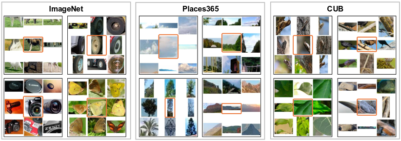
Figure 3: Clustered proposals as concepts. We show four concept clusters for ImageNet, Places365, and CUB, illustrating that clustering concept proposal embeddings produce semantically coherent clusters across datasets. The center image (orange border) represents the final concept (median image) for each cluster of concept proposals (created with SAM2, ViT L/14).

4.2.1 Concept clustering

We assess whether concept proposals form cohesive clusters whose median forms a meaningful concept for the CBM. Figure 3 shows that various representations of the same concept are clustered into a single concept.

These sample images demonstrate strong semantic coherence within clusters across all three datasets. Additionally, the plot illustrates the diversity of concepts captured within each dataset; for instance, ImageNet spans a wide range of object-centered categories, from animals to objects. Depending on the object’s complexity, these objects appear either as complete instances or a part thereof. In contrast, Places365’s scenes are more cluttered and less object-centric. Hence, its concepts include mountain range formations and vegetation. The highly specific CUB dataset contains sub-parts (legs) as well as complex clusters (bird on a tree trunk, vertically). This further confirms that the same foundation model can generate dataset-specific concept proposals suitable to train individual GCBMs.

4.2.2 Visual and semantic concept alignment

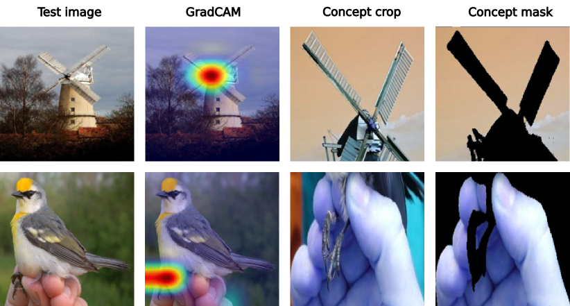
Figure 4: Grounded concepts. GCBM concepts can be grounded in the test images to deepen the model interpretability. We report Places365’s windmill [53] in row 1 and CUB’s Golden Wingend Warbler [46] in row two (created with SAM2, CLIP-RN50).

The visual and semantic alignment of GCBM concepts can be visualized using attribution methods. Figure 4 shows the test images (1. column), where the concepts (3. / 4. column) are located on the image (2. column). This way, visual concepts can be mapped back to the image to confirm that our interpretation of a concept is equal to the model’s understanding. In these cases, the GradCAM activation is where we expect it. It is also possible that the model detects a concept at an unexpected location in the image, thus offering us insights into the model’s inner workings.

4.3 CBM performance

We evaluate GCBMs both on the standard CBM datasets and beyond. The CBM performance on ImageNet-R, MiT-States, and ClimateTV confirms the generalization capabilities of the image concepts.

4.3.1 CLIP CBM comparison

In Tab. 1, we quantitatively evaluate the performance (top 1 accuracy) of GCBM against recent CBM approaches. Each experiment includes a linear probe and zero-shot accuracy, with an asterisk (*) indicating performances reported in prior literature. The dash (-) indicates no reported accuracies. The best result for each CLIP backbone and dataset is highlighted in bold. Hyperparameters are adjusted to $k=4096$ for ImageNet and $k=256$ for CIFAR-10 to reflect dataset sizes.

Model	CLIP ViT L/14
	IMN	Places	CUB	Cif10	Cif100
Linear Probe $\uparrow$	83.9*	55.4	85.7	98.0*	87.5*
Zero-Shot $\uparrow$	75.3*	40.0	0.7	96.2*	77.9*
LF-CBM [3] $\uparrow$	-	49.4	80.1	97.2	83.9
LaBo [7] $\uparrow$	84.0*	-	-	97.8*	86.0*
CDM [8] $\uparrow$	83.4*	55.2*	-	95.9	82.2
DCLIP [2] $\uparrow$	75.0*	40.5*	63.5*	-	-
DN-CBM [5] $\uparrow$	83.6*	55.6*	-	98.1*	86.0*
GCBM-SAM2 (Ours) $\uparrow$	77.9	52.1	81.8	97.7	85.4
GCBM-GDINO (Ours) $\uparrow$	77.4	52.2	81.3	97.5	85.3
GCBM-MASK-RCNN (Ours) $\uparrow$	77.8	52.1	82.4	97.7	85.6

Table 1: CBM benchmark. Performance comparison across different models and CLIP ViT L/14 on the benchmark datasets. The highest accuracies are bolt. Evaluation on the common benchmarks ImageNet [52], Places365 [53], CUB-200-2011 Caltech Birds [46], Cifar-10, and CIFAR-100 [51].

Our quantitative evaluation demonstrates that the GCBM approach achieves competitive performance. Our technique consistently delivers strong results across various datasets, particularly excelling in tasks such as CUB-200-2011, outperforming prior CBM methods. While GCBM approaches slightly lag behind state-of-the-art methods in specific benchmarks such as ImageNet, they maintain robust performance across the board. For all concept proposal generation methods (SAM2, GDINO, and MASK-RCNN), GCBMs performance is comparable, highlighting the adaptability and effectiveness of our methodology in grounding concepts to image regions. Appendix E contains experiments with additional CLIP backbones.

4.3.2 Generalization of GCBM concepts

Table 2 illustrates the generalization capabilities of the GCBM model trained on the ImageNet dataset with CLIP-RN50 embeddings. The model was evaluated on ImageNet-R (IN-R) [57], a subset containing 200 ImageNet classes in various renditions (e.g. embroidery, painting, comic). This dataset was created to assess model robustness to distribution shifts. In contrast to IN-R evaluations [57], which train the model exclusively on the classes evaluated in IN-R, we train the GCBM on all 1,000 ImageNet classes. We report the error rates for both the original ImageNet-200 and ImageNet-R datasets for the ResNet-based architectures [57].

	IN	IN-R	Gap(%)
ResNet-50 [57] $\downarrow$	7.9	63.9	56.0
ResNet-152 [57] $\downarrow$	6.8	58.7	51.9
GCBM-SAM2 (Ours) $\downarrow$	41.8	80.3	38.5
GCBM-GDINO (Ours) $\downarrow$	42.6	80.5	37.9
GCBM-MASK-RCNN (Ours) $\downarrow$	41.4	80.2	38.8

Table 2: GCBM ood performance. Error rates of different GCBM concept sets, trained on ImageNet and evaluated on the ImageNet-R (IN-R) [57]. The results demonstrate GCBM’s capability to generate concepts that produce accurate predictions on a related dataset. In contrast to IN-R evaluations [57], we train on all 1000 IN classes (emb. space: CLIP-RN50).

The accuracy drops as expected when evaluating on an ood dataset. While CBM performance is generally lower compared to IN fine-tuned models, we observe a significantly smaller drop in performance for GCBM than for the baseline ResNet. This smaller gap indicates that GCBM concepts can be used on ood domains.

In Section 4.1, we introduced two novel datasets, MIT-States [55] and ClimateTV [54], to further evaluate the generalization of GCBMs. Table 3 presents the CBM accuracy, linear probe, and zero-shot classification performance, all trained on the CLIP ViT L/14 backbone. GCBM performs better on ClimateTV, outperforming linear probes and zero-shot baselines. Additionally, for MIT-States, GCBM achieves better results than the linear probe approach. These results demonstrate the robustness of GCBM in capturing complex visual and semantic relationships, enabling it to generalize effectively across diverse datasets.

Method	MIT-States $\uparrow$	ClimateTV $\uparrow$
Linear Probe [57]	37.3	84.5
Zero-Shot [57]	48.1	69.7
GCBM-SAM2 (Ours)	42.8	85.6
GCBM-GDINO (Ours)	43.3	81.8
GCBM-MASK-RCNN (Ours)	43.2	87.9

Table 3: Generalization of GCBM. Test accuracy scores are reported for MIT-States and ClimateTV, including linear probe and zero-shot performance using the ViT L/14 backbone.

4.4 GCBM interpretability

We designed GCBMs to provide insights into model decision-making. Here, we qualitatively analyze and interpret the various explanations generated by our approach.

4.4.1 Qualitative analysis

In the following, we present sample interpretations generated using GCBMs. We examine one example each from the ImageNet, Places365, and CUB datasets. These evaluations are conducted on the CLIP ViT L/14 backbone, with SAM2 serving as the concept proposal model. For each instance, we show the input image along with the five most important concepts according to the CBM. Each concept is displayed alongside its name, based on a mapping with the g20k name space (Sec. 3.3). We divide this investigation into two parts: in Fig. 5, we analyze correct predictions, and in Fig. 6, we examine misclassifications.

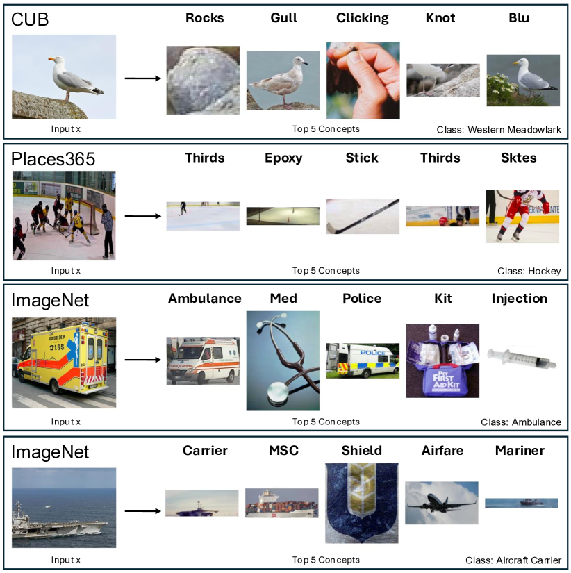
Figure 5: GCBM correct predictions. Concepts provide insights into the model’s embedding space, as it returns visually and/or semantically aligned concepts (SAM2 and ViT L/14).

The examples demonstrate the correct predictions and showcase concepts from each dataset that closely align with the semantics of the input image (see Eq. 3). The majority of concepts are visually and semantically aligned, as the hockey (Place365) image’s most important concepts are ice, (hockey) stick, sk(a)tes. However, not all activated concepts are visually present in the image. For instance, in the case of the ambulance image from ImageNet, concepts such as med, police, kit, or injection are not explicitly visible in the input image. This provides insights into the model’s embedding space, where a stethoscope is so similar to an ambulance, that it is the second most important concept. The second ImageNet instance depicts an aircraft carrier along with visually and semantically aligned image concepts. Visual and semantic alignment appears to differ depending on the concept at hand. Moreover, these examples showcase the quality of the concept naming. For Places365, the concept name thirds refers to the sport hockey being played in 3 thirds of 20 minutes.

The CBM misclassifications in Fig. 6 illustrate the interpretive plausibility of the GCBM’s classifications, with the top five visual concepts providing meaningful insights despite the ambiguity of the correct label. Especially the orange fruit in the Places365 example invites to classify this image as a vegetable garden rather than a botanical garden. Similar arguments can be found for the ImageNet example. The GCBM concepts allow to understand the model misclassifications better.

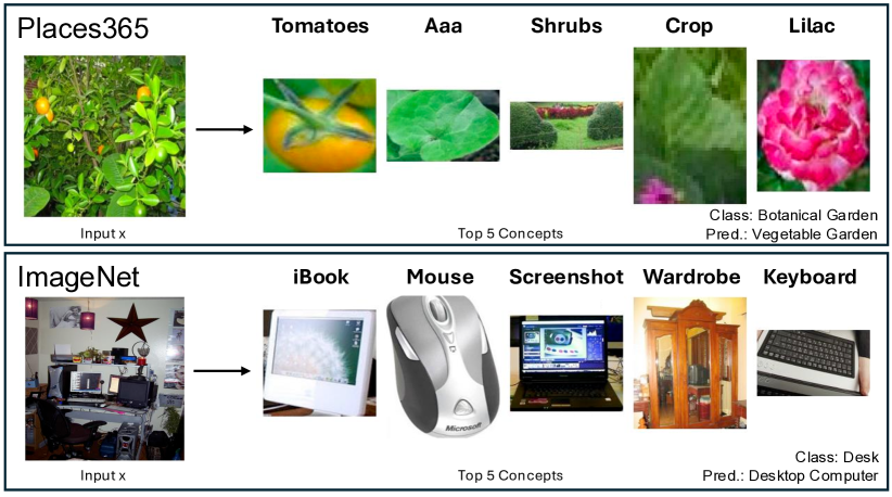
Figure 6: GCBM false predictions. Complex visual classes remain challenging, as the concepts could be mapped to both the correct and incorrect labels (SAM2 and ViT L/14).

4.4.2 CBM concept comparison

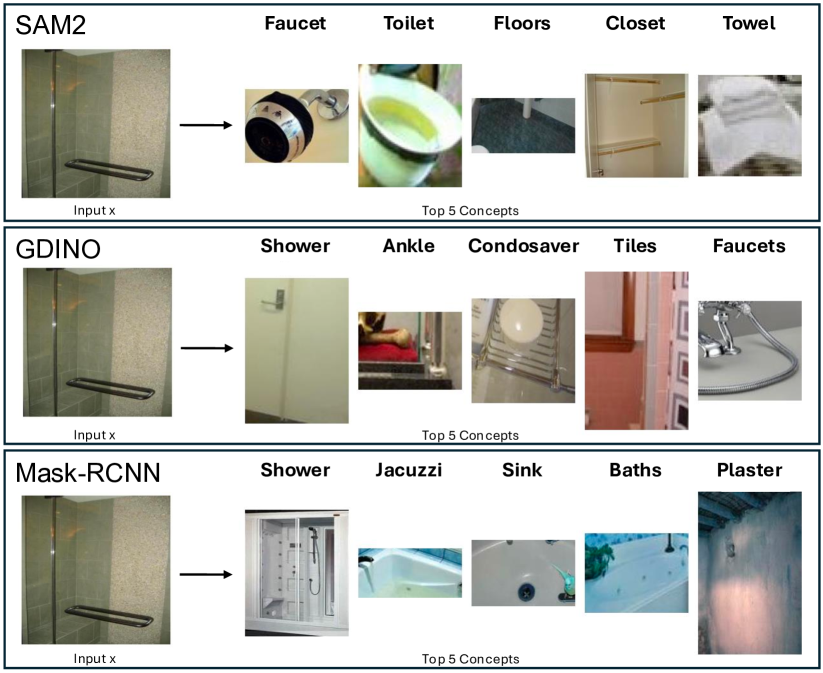
Figure 7: Diverse concept proposals. Concept sets differ in terms of granularity depending on segmentation or detection method employed, shown on shower (Places365).

The choice of concept proposal model determines the retrieved concept set. The generic SAM2 model creates a large number of concept proposals of all image elements, while Mask-RCNN returns object-centric concepts. In contrast, the promptable GroundingDINO is specifically steered to detect common object parts. While the different concept sets only differ marginally in terms of accuracy, as shown in Tab. 1 and Tab. 2, the interpretability is highly influenced. Here, we examine on Places365 with CLIP ViT L/14 the top five image concepts in Fig. 7. The figure displays interpretations for the same input image, correctly classified as shower by all three models, with each concept image accompanied by the closest matching textual label (g20k name space). The image activates consistently concepts that exhibit semantic alignment with the class shower or the larger context of the bathroom, where towels, faucets, sinks, and bath (tubs) can commonly be found. In particular, GroundingDINO (GDINO) and Mask-RCNN produce top concepts that closely match CLIP’s textual embedding for the shower, even though both concepts appear quite different, as the Mask-RCNN concept resembles a shower, while GDINO’s concept corresponds to an image of a door.

5 Discussion & Conclusion

With GCBMs, we create a simple, efficient, and dataset-specific framework for model interpretability, which can easily be adapted to new datasets. Using segmentation and detection foundation models, we retrieve image-inherent concepts, without any LLM interference. For any CBM predictions, we can visually inspect the most important and trace their activations back to the input image.

5.1 Discussion

GCBM’s accuracy is in all experiments within 5% of the linear probe, which indicates that GCBM is a comparable alternative to the other CBM methods. Given the recent trend of CBMs using the CLIP embedding space, we focus our quantitative comparison on such models exclusively. Overall, all CBM methods achieve the lowest performance on Places365, which may be partly due to the visual similarity of several dataset classes, as reported in Fig. 6. When comparing our work to the pure CNN methods Schrodi et al. [6], we discuss the performance differences between datasets rather than concrete classification accuracies. The relative performance of different CBM approaches differ, with several methods performing better in ImageNet than CUB [2, 6]. Rao et al. [5] do not report their CUB performance, but their outlook proposes pre-training on larger datasets to enhance fine-grained classification. GCBMs performance on CUB is consistently superior to its performance on ImageNet, indicating the strength of our approach. On top of that, GCBMs can easily be used for new datasets, as they achieve accuracies similar to linear probes (Sec. 4.3.2).

Qualitative concept analysis (Sec. 4.4) shows that GCBM concepts contain parts of the dataset’s classes. However, Fig. 5 and Fig. 7 highlight that within the CLIP embedding space, semantically close concepts may be activated without being present in the input image. This peculiarity cannot only be observed in our examples, but also within all other CLIP CBMs [5, 3, 8, 7, 2]. While this allows for interesting insights into the CLIP embedding space, it also raises the question of its usefulness for CBMs. Attribution methods such as GradCAM can visualize these semantic similarities between visually different concepts. In CBMs without LLM integration, we can be sure that such visual mismatches are due to the construction of the embedding spaces. Given textual concepts, such visual variations of a single semantic concept would be less apparent, as the concepts are not visually inspectable, only their closest representations can be accessed.

Efficiency is a clear strength of GCBMs since they do not require general [5] or dataset-specific pre-training [6]. The concept proposal set is created on a subset of 50 images per class as standard; fewer images may be used in a trade-off for accuracy. Additionally, GCBMs do not require general nor dataset-specific pre-training of any sort, thus making the adaptation to new datasets is easily possible.

5.2 Limitations & Future Work

During cluster investigation, we found similar or redundant concepts, giving room for further optimization during or after clustering. The ideal clustering contains all existing concepts only once. In practice, this is hard to achieve, given the different levels of variation between concepts. Current GCBM concepts sometimes contain a mismatch between visual and semantic concepts. These mismatches are reported by all CLIP-based CBM models and need to be further investigated. Additionally, other embedding spaces can be evaluated to discuss inter-model differences. We assume that vision embedding spaces would reduce the number of visually disjoint-matched concepts. We can further benefit from advances in the field of segmentation and detection models, as new methods can easily be integrated within the GCBM framework. Similarly, the GCBM framework can easily be adapted to other CBM architectures. For instance, CBM sparsity can be further increased, as this increases model interpretability at the cost of accuracy [6].

5.3 Conclusion

In this work, we present visually Grounded Concept Bottleneck Models (GCBM), a novel approach to CBMs that uses image-level concepts, which can be visually grounded in the input image. GCBMs employ a simple and intuitive approach to deriving image concepts by using segmentation or detection foundation models. Clustering concept proposals, reduces the different representations of concepts to a single prototypical one, which is used for CBM training and evaluation. Having visual representations of concepts, the CBM makes visual and semantic mismatches apparent. GCBM’s efficient and unrestricted adaptability to other datasets highlights its potential as a general-purpose CBM framework, paving the way for future research into interpretable models that link human-understandable concepts with visual data. Our approach generalizes well across domains and datasets, demonstrating robustness with segmentation techniques like SAM2, Grounding DINO, and MASK-RCNN, establishing it as a versatile framework. Given that no pre-training is required, GCBMs can provide interpretations for a new dataset in under one hour (depending on dataset size).

Supplementary Material

Appendix A Dataset overview and details

A.1 Ablations

We ablate on three datasets: ImageNette [49], ImageWoof [50], and CUB [46]. The first two datasets are both subsets of ImageNet [52]. ImageNette contains easier-to-classify categories like tench, English springer, and church. ImageWoof images focus on dog breeds, curated for fine-grained classification tasks. The Caltech-UCSD Birds 200 dataset is designed to identify fine-grained bird species with detailed annotations. For the datasets which do not have a test split, we use the validation split for testing and create a new split, i.e. 10% of train set, for validation. Consequently, the train split comprises only 90% of the original train images.

Dataset	Classes	Images
		%(train / val / test)
ImageNette	10	13,000 (70 / 30 / 0)
ImageWoof	10	12,000 (70 / 30 / 0)
CUB-200-2011	200	11,788 (50 / 50 / 0)

Table 4: Ablation datasets. Overview of the datasets used for ablation (ImageWoof, ImageNette, and CUB-200-2011).

A.2 Benchmark analysis

For the primary analysis, we compare five datasets: Imagenet [52], Places365 [53], CUB [46], cifar10 and cifar100 [51]. For ImageNet, we report on the validation split. Thus, we use it as our test set. Again, we create a small validation set to select the hyperparameters on an independent dataset in situations where we cannot access three labelled splits.

Dataset	Classes	Images
		%(train / val / test)
ImageNet	1,000	1,431,167 (90 / 3 / 7)
Places365	365	1,839,960 (98 / 2 / 0)
CUB-200-2011	200	11,788 (50 / 50 / 0)
CIFAR-10	10	60,000 (83 / 0 / 17)
CIFAR-100	100	60,000 (83 / 0 / 17)

Table 5: Main datasets. Overview of the datasets used for benchmark experiments (ImageNet, Places365, CUB, CIFAR-10, and CIFAR-100).

A.3 Additional datasets

We use three datasets which are novel to the CBM research: MiT-States [55], Climate-TV [54], and ImageNet-R [57]. MiT-States contains images of 245 object classes in combination with 115 attributes. This allows the assessment of concept recognition in previously unseen shapes or former, as the test set contains 50% seen and 50% unseen versions of objects e.g. ripe tomato, unripe tomato, moldy tomato. We evaluate the accuracy of the object class. Thus, we use this dataset to assess whether we can detect an object independent of its state. We use the train-val-test split (30k-10k-13k) introduced by [58]. ClimateTV contains social media images of climate change and includes a diverse range of images. We have created a balanced set for the animals-superclass, which contains 11 animal classes, including ”no animals”. This allows the assessment of real-life images, which are, by design, messier than curated datasets.

Dataset	Classes	Images
		%(train / val / test)
MiT-States	245	53,743 (57 / 19 / 24)
ClimateTV	11	660 (80 / 0 / 20)
ImageNet-R	200	30,000 (0 / 100 / 0)

Table 6: Additional datasets. Overview of the additional dataset (MiT-States, CliamteTV, and ImageNet-R).

ImageNet-R consists of 200 ImageNet classes and is generally used to evaluate ood performance of a model trained on ImageNet. The ”R” stands for renditions of which the dataset contains cartoons, graffiti, embroidery, graphics, origami, paintings, and many more [57]. This task is simplified by training the model exclusively on the 200 classes of ImageNet-R. In our case, however, we report the model’s performance when trained on all ImageNet classes.

Appendix B Concept proposal generation

We provide the code for all segmentation methods employed and make it publicly available. Tab. 7 provides an overview of the segmentation models’ hyperparameters, which are unchanged for MaskRCNN and DETR compared to the pre-trained models. Hyperparameters were set to retrieve concept proposals that break the image into sub-parts. For GroundingDino, we evaluated two thresholds to compare whether a more, noisier concept proposal or a fewer, cleaner concept proposal performed better.

Segmentation model	Hyperparameters
SAM	points_per_side = $64$,
	pred_iou_thresh = $0.88$,
	stability_score_thresh = $0.95$,
	box_nms_thresh = $0.5$,
	min_mask_region_area = $500$
SAM2	points_per_side = $64$,
	pred_iou_thresh = $0.88$,
	stability_score_thresh = $0.95$,
	box_nms_thresh = $0.5$,
	min_mask_region_area = $500$
	min_mask_region_area = $500$
GDINO	box_threshold = $[0.35,0.25]$,
	text_threshold = $0.25$

Table 7: Hyperparameters of segmentation models. We only report model hyperparameters if we change them compared to the standard setting.

B.1 Prompts

For the promptable GroundingDINO model, we assess the efficacy of several prompts w.r.t. CBM performance. To this end, we use attribute or part labels, which have been published in other contexts, thus avoiding manual or LLM-based concept set generation. We use the part annotations for CUB [46], the attributes for Animals with Attributes (GDINO Awa) [42], and standard part-labels from Part-ImageNet [44] and GDINO Pascal-PARTS [43].

Model	CLIP ResNet-50			CLIP ViT-B/16			CLIP ViT-L/14
	ImageNette	ImageWoof	CUB	ImageNette	ImageWoof	CUB	ImageNette	ImageWoof	CUB
SAM w/o	98.55	90.96	57.04	99.57	93.66	71.68	99.87	95.42	80.03
SAM w/	98.50	90.81	57.62	99.54	93.79	73.44	99.80	97.78	79.58
SAM2 w/o	98.73	91.70	59.89	99.52	94.38	73.61	99.87	95.75	80.98
SAM2 w/	98.78	91.68	61.44	99.57	94.30	75.49	99.85	95.80	82.21
MaskRCNN w/o	98.65	91.93	64.62	99.59	94.38	77.60	99.80	95.70	83.60
MaskRCNN w/	98.68	91.89	65.46	99.59	94.60	77.61	99.82	95.65	83.32
DETR w/o	98.65	91.80	64.17	99.46	94.45	76.84	99.82	95.75	82.57
DETR w/	98.73	92.03	61.18	99.54	94.58	76.91	99.80	95.78	82.52

Table 8: Background performance influence. Performance comparison with (w/) and without (w/o) background on the ablation datasets.

Appendix C Ablations

We conduct ablation studies to evaluate GCBM’s performance under various hyperparameters and configurations. These studies are performed on the ImageNette, ImageWoof, and CUB to identify settings that yield strong performance across all three datasets. The identified configurations are used for the main experiments presented in Sec. 4. Each GCBM was trained with 1024 clusters, using K-Means clustering with the median of each cluster as a concept, a learning rate of $1e{-4}$, and sparsity regularization set to $1e{-4}$. We explore a broader range of segmentation and object detection models beyond those discussed in the main paper, such as SAM and extended prompts for GDINO. The ”Low” label indicates a low threshold for the corresponding object detection configuration. What differentiates these experiments from those in the main paper is the use of PCA, reducing the dimensionality of concept proposals to 100. This approach accelerates clustering and enables more efficient experimentation. Additionally, we investigate the impact of PCA on the performance of GCBM.

C.1 Background removal

The background influences embedding the image regions used as concepts for the segmentation methods employed. To assess this effect, we examine accuracies in Tab. 8 using three different CLIP embeddings: ResNet-50, ViT B/16, and ViT L/14 — while excluding the background concept, based on ImageNette, ImageWoof, and CUB. We report SAM, SAM2, Mask R-CNN, and DETR results. Each model was trained with a learning rate of $1e{-4}$, a lambda of $1e{-4}$, 128 clusters using median and k mean, and 50 images per class within the GCBM framework.

C.2 PCA

C.2.1 Cluster similarities

	ResNet-50	CLIP ViT-B/16	CLIP ViT-L/14
GCBM-SAM2 (Ours) w	61.2	75.1	81.9
GCBM-SAM2 (Ours) w/o	61.4	75.3	81.8
GCBM-GDINO (Ours) w	58.9	73.9	81.1
GCBM-GDINO (Ours) w/o	59.0	74.1	81.3
GCBM-MASK-RCNN (Ours) w	64.6	76.8	82.
GCBM-MASK-RCNN (Ours) w/o	64.6	76.7	82.4

Table 9: Impact of PCA on CUB dataset. Accuracy comparison of GCBM with and without PCA (100 components) evaluated on the CUB dataset.

To assess the impact of different hyperparameter settings within the GCBM framework, we analyze clustering similarities across various values of $k$ in K-means and compare these results across different CLIP backbone models in Figure 8(a). Our primary focus is on the CUB dataset, as its exclusive focus on bird images introduces ambiguity in clustering compared to other datasets. Additionally, in Fig. 8(b), we examine the effect of applying PCA with 100 components to the segment embeddings before clustering to determine whether this transformation yields similar clustering outcomes. For this evaluation, we use the NMI (Normalized Mutual Information) metric, where an NMI score close to 1 indicates high similarity, meaning that the two clustering approaches capture comparable groupings or structures. In contrast, a score near 0 suggests minimal alignment, indicating substantially different clustering results.

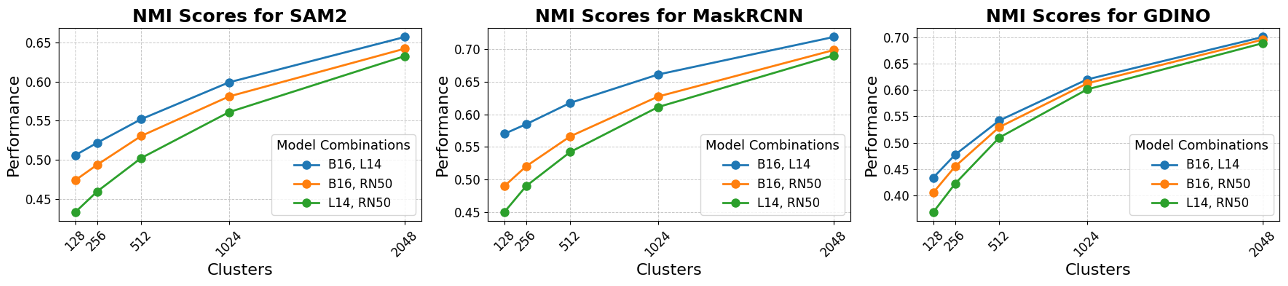
(a) Backbone NMI scores. NMI scores for three CLIP model combinations: B16, L14 (blue), B16, RN50 (orange), and L14, RN50 (green), showing clustering performance across different backbones.

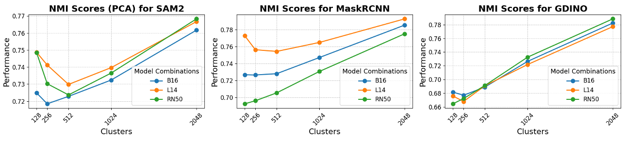
(b) PCA NMI scores. NMI scores illustrate clustering consistency with and without PCA preprocessing for each CLIP backbone.

Figure 8: NMI scores for the CUB dataset. The plots present NMI (Normalized Mutual Information) scores for SAM2, MaskRCNN, and GDINO models across varying cluster sizes (128, 256, 512, 1024, 2048) on the CUB dataset. (a) Backbone NMI Scores: shows clustering similarities across different CLIP backbone combinations. (b) PCA NMI Scores: compares clustering consistency with and without applying PCA (100 components) before clustering.

As shown in Fig. 8(a), the B16, L14 combination consistently achieves the highest NMI scores. Additionally, as the number of clusters $k$ increases, the NMI scores improve in all segmentation techniques and backbone combinations, indicating that larger cluster sizes capture more meaningful distinctions in the data. These results suggest concept clusters remain similar across different CLIP backbones, with minimal unique variation among specific backbone combinations.

Similarly, Fig. 8(b) illustrates the impact of PCA on cluster similarity. While PCA reduces dimensionality and speeds up the clustering process, the clusters formed remain broadly consistent with those generated without PCA. This suggests that PCA minimally affects the conceptual alignment within CBMs, preserving the overall clustering structure. Furthermore, as demonstrated in Tab. 9 for CUB, this limited influence extends to the overall performance of GCBMs.

C.3 Clustering algorithm

We evaluate two clustering algorithms in the main ablation study: hierarchical clustering and K-means. The results, presented in Tab. 10, are based on a consistent configuration where the median centroid is used, and the number of clusters $k$ is fixed at 1024 across all datasets. While the performance scores of both methods are generally comparable, K-means slightly outperforms hierarchical clustering in most cases. Consequently, we use K-means for the main experiments.

Model	Clustering Method	CLIP ResNet-50			CLIP ViT-B/16			CLIP ViT-L/14
		ImageNette	ImageWoof	CUB	ImageNette	ImageWoof	CUB	ImageNette	ImageWoof	CUB
SAM	Hierarchical	98.60	90.74	61.15	99.52	93.38	73.27	99.82	95.65	82.11
	K-means	98.52	90.86	57.62	99.57	93.74	73.44	99.82	95.90	80.03
SAM2	Hierarchical	98.75	92.11	61.15	99.62	94.45	75.39	99.85	95.80	82.12
	K-means	98.72	92.19	61.44	99.59	91.60	75.60	99.85	95.70	81.88
DETR	Hierarchical	98.73	92.03	63.96	99.54	94.53	76.82	98.77	95.85	82.31
	K-means	98.65	92.21	64.27	99.54	94.60	77.01	99.80	95.80	82.64
MaskRCNN	Hierarchical	98.68	92.03	65.41	99.57	94.35	77.53	99.85	95.78	83.21
	K-means	98.73	91.86	65.46	99.60	94.60	77.70	99.85	95.65	83.33
GDINO Awa	Hierarchical	98.57	91.27	58.54	99.41	93.99	74.13	99.87	95.70	81.36
	K-means	98.50	91.17	57.97	99.46	94.04	73.63	99.89	95.60	81.12
GDINO Awa Low	Hierarchical	98.60	90.81	57.84	99.44	94.15	73.92	99.87	95.62	81.17
	K-means	98.57	90.91	65.43	99.41	94.17	77.70	99.87	95.67	83.09
GDINO Partimagenet	Hierarchical	98.47	91.30	59.30	99.39	94.12	74.30	99.80	95.54	81.14
	K-means	98.47	91.27	59.63	99.44	94.17	74.70	99.82	95.62	81.52
GDINO Partimagenet Low	Hierarchical	98.55	90.76	58.99	99.46	94.25	74.44	99.82	95.55	81.14
	K-means	98.52	90.99	59.39	99.52	94.17	74.20	99.85	95.83	81.22
GDINO Pascal	Hierarchical	98.60	90.81	58.77	99.44	94.15	73.66	99.87	95.62	80.74
	K-means	98.57	90.91	58.80	99.41	93.17	73.73	99.87	95.67	81.00
GDINO Pascal Low	Hierarchical	98.62	90.84	58.37	99.49	94.10	73.97	99.85	95.75	81.03
	K-means	98.62	90.89	58.25	99.52	93.89	73.78	99.85	95.75	81.15
GDINO Sun	Hierarchical	98.09	83.10	58.85	99.16	88.90	73.70	99.62	93.40	80.95
	K-means	98.16	82.97	58.85	99.18	88.78	73.77	99.62	93.54	81.00
GDINO Sun Low	Hierarchical	98.60	90.94	58.94	99.47	93.79	74.42	99.82	95.88	81.36
	K-means	98.60	90.94	59.00	99.47	94.46	74.54	99.80	95.88	81.51

Table 10: Clustering method comparison. Performance comparison of different clustering algorithms (Hierarchical and K-Means), both with $k$ set to 1024.

Additionally, we tested DBSCAN and HDBSCAN. However, these methods required significant hyperparameter tuning to achieve meaningful clusters. In contrast, K-means and hierarchical clustering required only the definition of $k$. We leave this analysis for future work.

C.4 Centroid

After clustering the concept proposals $\mathcal{S}$ into $k$ clusters, a centroid is generated for each cluster to represent it. We evaluate the impact of using two different methods to compute centroids: the mean of the embeddings within a cluster and the median embedding, as shown in Tab. 11. This analysis is applied to both integrated clustering techniques while keeping all other configurations consistent with the standard settings. In the main paper, we reference this section with a previous name (Tab. 4). We will update this in the camera-ready version. Overall, the K-means configuration using the median centroid performs the best across the three datasets. While there are specific scenarios where other combinations yield better results, we adopt this standard setting for simplicity following this investigation.

Model	Clustering Method	Centroid	CLIP ResNet-50			CLIP ViT-B/16			CLIP ViT-L/14
			ImageNette	ImageWoof	CUB	ImageNette	ImageWoof	CUB	ImageNette	ImageWoof	CUB
SAM	Hierarchical	Mean	98.45	89.62	56.78	99.44	92.95	68.66	99.75	95.39	80.34
	Hierarchical	Median	98.60	90.74	61.15	99.52	93.38	73.27	99.82	95.65	82.11
	K-means	Mean	98.42	89.67	48.64	99.46	93.03	69.33	99.77	95.37	76.49
	K-means	Median	98.52	90.86	57.62	99.57	93.74	73.44	99.82	95.90	80.03
SAM2	Hierarchical	Mean	98.73	92.03	56.78	99.57	94.42	73.11	99.85	95.75	80.34
	Hierarchical	Median	98.75	92.11	61.15	99.62	94.45	75.39	99.85	95.80	82.12
	K-means	Mean	98.73	92.20	56.63	99.59	91.60	73.30	99.82	95.83	80.19
	K-means	Median	98.72	92.19	61.44	99.59	91.60	75.60	99.85	95.70	81.88
DETR	Hierarchical	Mean	98.68	92.11	63.46	99.54	94.50	76.46	99.80	95.75	82.00
	Hierarchical	Median	98.73	92.03	63.96	99.54	94.53	76.82	98.77	95.85	82.31
	K-means	Mean	98.68	92.19	63.27	99.54	94.52	76.23	99.80	95.80	81.69
	K-means	Median	98.65	92.21	64.27	99.54	94.60	77.01	99.80	95.80	82.64
MaskRCNN	Hierarchical	Mean	98.70	91.65	63.07	99.59	94.48	76.75	99.79	95.62	82.41
	Hierarchical	Median	98.68	92.03	65.41	99.57	94.35	77.53	99.85	95.78	83.21
	K-means	Mean	98.75	91.73	63.00	99.59	94.63	77.13	99.82	95.62	82.22
	K-means	Median	98.73	91.86	65.46	99.60	94.60	77.70	99.85	95.65	83.33
GDINO Awa	Hierarchical	Mean	98.57	91.14	52.54	99.44	94.02	70.59	99.85	95.78	78.60
	Hierarchical	Median	98.57	91.27	58.54	99.41	93.99	74.13	99.87	95.70	81.36
	K-means	Mean	98.62	91.07	53.00	99.41	93.97	70.92	99.87	95.70	79.00
	K-means	Median	98.50	91.17	57.97	99.46	94.04	73.63	99.89	95.60	81.12
GDINO Awa Low	Hierarchical	Mean	98.60	90.61	50.31	99.44	93.87	69.95	99.87	95.83	78.25
	Hierarchical	Median	98.60	90.81	57.84	99.44	94.15	73.92	99.87	95.62	81.17
	K-means	Mean	98.52	90.79	63.00	99.39	93.94	77.13	99.90	95.57	82.22
	K-means	Median	98.57	90.91	65.43	99.41	94.17	77.70	99.87	95.67	83.09
GDINO Partimagenet	Hierarchical	Mean	98.44	90.99	53.57	99.41	94.17	71.35	99.80	95.57	79.01
	Hierarchical	Median	98.47	91.30	59.30	99.39	94.12	74.30	99.80	95.54	81.14
	K-means	Mean	98.47	91.19	53.92	99.39	94.10	71.54	99.82	95.57	78.79
	K-means	Median	98.47	91.27	59.63	99.44	94.17	74.70	99.82	95.62	81.52
GDINO Partimagenet Low	Hierarchical	Mean	98.42	90.63	52.42	99.46	94.20	70.66	99.85	95.60	78.20
	Hierarchical	Median	98.55	90.76	58.99	99.46	94.25	74.44	99.82	95.55	81.14
	K-means	Mean	98.42	90.68	51.97	99.49	94.30	70.56	99.84	95.62	78.12
	K-means	Median	98.52	90.99	59.39	99.52	94.17	74.20	99.85	95.83	81.22
GDINO Pascal	Hierarchical	Mean	98.60	90.60	51.00	99.44	93.86	70.02	99.87	95.82	77.99
	Hierarchical	Median	98.60	90.81	58.77	99.44	94.15	73.66	99.87	95.62	80.74
	K-means	Mean	98.52	90.79	50.95	99.39	93.94	70.26	99.90	95.57	77.93
	K-means	Median	98.57	90.91	58.80	99.41	93.17	73.73	99.87	95.67	81.00
GDINO Pascal Low	Hierarchical	Mean	98.62	90.43	50.17	99.46	93.84	69.66	99.87	95.90	77.61
	Hierarchical	Median	98.62	90.84	58.37	99.49	94.10	73.97	99.85	95.75	81.03
	K-means	Mean	98.60	90.58	50.48	99.49	93.99	69.64	99.85	95.80	77.51
	K-means	Median	98.62	90.89	58.25	99.52	93.89	73.78	99.85	95.75	81.15
GDINO Sun	Hierarchical	Mean	98.11	82.77	58.53	99.13	88.52	73.71	99.62	93.33	80.91
	Hierarchical	Median	98.09	83.10	58.85	99.16	88.90	73.70	99.62	93.40	80.95
	K-means	Mean	98.09	83.13	58.72	99.13	88.62	73.66	99.57	93.54	80.84
	K-means	Median	98.16	82.97	58.85	99.18	88.78	73.77	99.62	93.54	81.00
GDINO Sun Low	Hierarchical	Mean	98.50	90.94	54.49	99.49	93.71	72.39	99.82	95.69	79.43
	Hierarchical	Median	98.60	90.94	58.94	99.47	93.79	74.42	99.82	95.88	81.36
	K-means	Mean	98.55	90.91	54.80	99.49	93.43	72.61	99.80	95.75	80.00
	K-means	Median	98.60	90.94	59.00	99.47	94.46	74.54	99.80	95.88	81.51

Table 11: Centroid selection: mean vs. median. This figure illustrates the comparative analysis of centroid selection methods — mean and median — on hierarchical and K-means clustering performance.

C.5 Number of clusters

As described in Sec. 3, we cluster the concept proposal set $\mathcal{S}$ into $k$ clusters. The choice of $k$ determines the granularity of the concepts used in the GCBM method. To analyze this, we test various values of $k$ within the K-Means algorithm, as shown in Tab. 15, presenting an ablation study of $k$. We do not impose the 50-images-per-class limitation in these experiments due to the generally smaller number of images available per dataset and class. As the table illustrates, increasing the number of clusters leads to a corresponding improvement in accuracy scores, highlighting the benefit of finer-grained concept representations.

C.6 Lambda and learning rate

In Tab. 16 and Tab. 17, we analyze the impact of different hyperparameters for sparsity ($\lambda$) in Eq. 4 and the learning rate. To provide a more transparent overview, we present the results in two separate tables: Tab. 16 focuses on segmentation models, while Tab. 17 covers object detection models. All other configurations remain consistent with the settings reported earlier. From the results, the optimal configuration across the three datasets and various concept creation modules is a learning rate of $1e{-4}$ combined with a sparsity of $1e{-4}$. Although specific configurations demonstrate improved performance with alternative values, we aim to identify a baseline configuration that performs robustly across diverse scenarios.

C.7 Number of images per class

GCBM does not require using all images in a dataset to generate meaningful concepts. In this section, we evaluate the impact of varying the number of images per class (5, 10, 25, and 50) on the resulting accuracy using the standard configurations from the ablation study. The accuracy scores are presented in Tab. 18. Increasing the number of images per class most often leads to improved accuracy. However, the improvements become marginal beyond 25 images, with the difference between 25 and 50 being minimal. Consequently, we limited our investigation to 50 images per class to balance accuracy with computational efficiency, as a higher number of images requires more segmentation and object detection, significantly increasing computational costs with diminishing returns.

Appendix D Implementation details

Our implementation is in Python and Pytorch, and our CBM implementation is based on [47, 5]. For GradCAM [22] calculations, we use the implementation by [59], which we adjust to ViT’s and concept instead of text matching based on Gildenblat et al.’s implementation [60]. In the main paper, we reference this section with a previous name (Appendix B.2). We will update this in the camera-ready version.

Model	CLIP ResNet-50					CLIP ViT-B/16					CLIP ViT-L/14
	IMN	Places	CUB	Cif10	Cif100	IMN	Places	CUB	Cif10	Cif100	IMN	Places	CUB	Cif10	Cif100
Linear Probe	73.3*	53.4*	68.9	88.7*	70.3*	80.2*	55.1*	81.0	96.2*	83.1*	83.9*	55.4	85.7	98.0*	87.5*
Zero Shot	59.6*	37.9	0.8	75.6*	41.6*	68.6*	39.5*	0.9	91.6*	68.7*	75.3*	40.0	0.7	96.2*	77.9*
LF-CBM [3]	72.0*	46.8	74.3*	86.4*	65.1*	75.4	48.2	74.0	94.7	77.4*	–	49.4	80.1	97.2	83.9
LaBo [7]	68.9*	–	–	87.9*	69.1*	78.9*	–	–	95.7*	81.2*	84.0*	–	–	97.8*	86.0*
CDM [8]	72.2*	52.7*	72.3*	86.5*	67.6*	79.3*	52.6*	79.5*	95.3*	80.5*	83.4*	55.2*	–	95.9	82.2
DCLIP [2]	59.6*	37.9*	49.0	–	–	68.0*	40.3*	57.8*	–	–	75.0*	40.5*	63.5*	–	–
DN-CBM [5]	72.9*	53.5*	–	87.6*	67.5*	79.5*	55.1*	–	96.0*	82.1*	83.6	55.6	–	98.1	86.0
GCBM-SAM2 (Ours)	58.7	48.0	61.4	84.5	61.8	70.4	50.6	75.3	95.2	79.4	77.9	52.1	81.8	97.7	85.4
GCBM-GDINO (Ours)	58.7	47.8	59.0	83.9	61.2	69.7	50.7	74.1	95.1	79.6	77.4	52.2	81.3	97.5	85.3
GCBM-MASKRCNN (Ours)	58.7	48.2	64.6	84.5	62.7	70.5	50.9	76.7	95.2	79.6	77.8	52.1	82.4	97.7	85.6

Table 12: Extended CBM benchmark. Performance comparison across different CLIP versions on datasets used for ablation study. Hyperparameters correspond to the ones reported for ViT L14.

D.1 Efficiency and runtimes

The creation of concept proposals is influenced by the number of images per class and the foundation model used to generate outputs from these images. Consequently, the computational effort required for concept creation is highly dependent on the input characteristics, similar to other approaches that involve training a sparse autoencoder for concept generation [5], performing non-negative matrix factorization, or utilizing a large language model [7]. In the main paper, we provided rough estimations of the computation time required for concept creation within GCBM.

However, once the concepts are generated, we can directly compare the runtime per epoch between our framework and others on the same dataset. To illustrate this, we measured the runtime for a single epoch ImageNet using GCBM and DN-CBM, employing a 90/10 train-validation split and adhering to the standard hyperparameters specified in [5] and our work for GCBM. Both methods were evaluated on the same machine using ViT ResNet50 as the backbone. Our measurements reveal that a single epoch takes an average of 16 seconds for DN-CBM, while for GCBM, the average runtime per epoch is 9 seconds (with SAM2). This significant reduction in runtime for GCBM is attributed to fewer concepts, which reduces the input size to the linear model compared to DN-CBM.

Appendix E Quantitative results

E.1 CLIP backbones

We present the accuracies of additional CLIP backbones, ResNet-50 and ViT B/16, in Tab. 12. We used the same hyperparameters as those initially selected for ViT L/14 for consistency. While ViT B/16 performs competitively, ResNet-50 lags behind other CBM techniques. We attribute this disparity to ResNet-50’s limited capacity to capture complex semantic relationships compared to transformer-based models, better equipped to handle the nuanced contextual understanding required for this task.

E.2 Generalization of GCBM

In Tab. 2, we present the error rates of GCBM trained on ImageNet and evaluated on ImageNet-R using CLIP ResNet-50 (Res50). In contrast, Tab. 13 showcases the error rates for CLIP ViT-L/14, demonstrating superior performance owing to the enhanced representative capacity of the ViT-L/14 architecture. The performance gap decreases by a third, with overall error rates being substantially lower (ranging from -20 to -40) when using ViT-L/14 compared to ResNet-50 within the GCBM framework.

	IN	IN-R	Gap(%)
GCBM-SAM2 (Ours) $\downarrow$	21.1	48.5	27.4
GCBM-GDINO (Ours) $\downarrow$	22.6	47.2	24.6
GCBM-MASK-RCNN (Ours) $\downarrow$	22.2	44.6	22.4

Table 13: GCBM ood performance - ViT L14. Error rates of different GCBM concept sets, trained on ImageNet and evaluated on the ImageNet-R (IN-R) [57] with CLIP ViT L/14.

Additionally, we evaluate DN-CBM [5] under the same settings, training on all 1000 ImageNet classes and testing on ImageNet-R. The corresponding error rates differ much more for DN-CBM than for GCBM, as presented in Tab. 14. We also include GCBM’s error rates for comparison, using CLIP ResNet-50 as the backbone. Due to some bugs in DN-CBM’s code, we are only able to report these findings here and not in the main paper.

	IN	IN-R	Gap(%)
DN-CBM $\downarrow$	27.1	74.2	47.1
GCBM-SAM2 (Ours) $\downarrow$	41.8	80.3	38.5
GCBM-GDINO (Ours) $\downarrow$	42.6	80.5	37.9
GCBM-MASK-RCNN (Ours) $\downarrow$	41.4	80.2	38.8

Table 14: DN-CBM ood performance. Error rates for DN-CBM [5] and GCBM concept sets, trained on ImageNet and evaluated on ImageNet-R (IN-R) [57] using CLIP ResNet-50 as the backbone.

Appendix F Qualitative results

In the following, we provide additional explanations in Fig. 9, similar to those discussed in Sec. 4.4, focusing on the ablation datasets ImageWoof and ImageNette. These examples further highlight the effectiveness of GCBM on these specific datasets. Since both datasets consist of only ten classes each, the limited variety of concepts is likely a result of the reduced range of distinct concept proposals. This occurs because the datasets contain similar images representing closely related classes, leading to overlapping or redundant concept representations.

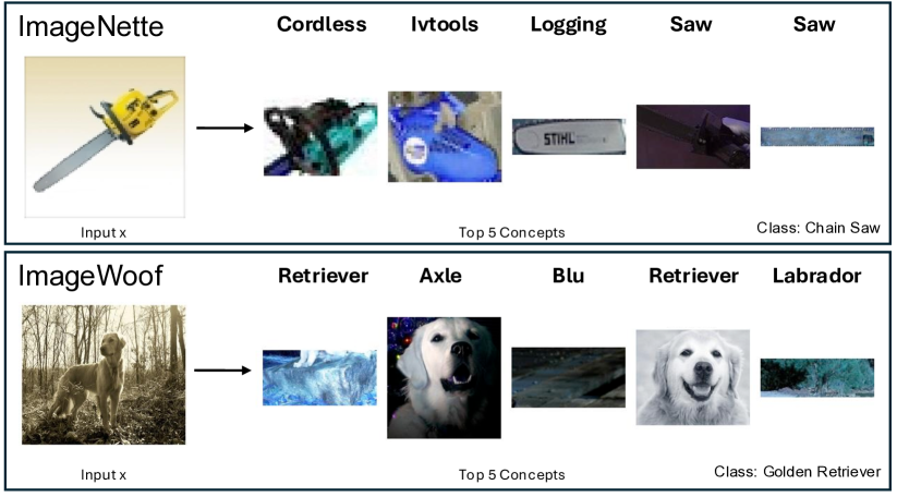
Figure 9: GCBM ablations. Our technique GCBM was applied to ImageWoof and ImageNette (SAM2 and ViT L/14).

Model	Clusters	CLIP ResNet-50			CLIP ViT-B/16			CLIP ViT-L/14
		ImageNette	ImageWoof	CUB	ImageNette	ImageWoof	CUB	ImageNette	ImageWoof	CUB
SAM	128	97.73	82.29	37.40	99.13	89.41	59.82	99.64	93.05	71.35
	256	98.27	86.77	46.58	99.31	92.08	68.61	99.80	95.06	76.61
	512	98.60	89.57	53.38	99.46	93.51	72.11	99.82	95.65	78.94
	1024	98.50	90.81	57.62	99.54	93.79	73.44	99.80	97.78	79.58
	2048	–	–	59.16	–	–	73.85	–	–	80.44
SAM2	128	98.22	87.02	44.68	99.36	92.19	65.29	99.80	95.50	75.56
	256	98.42	89.69	51.28	99.46	93.84	71.92	99.75	95.60	59.38
	512	98.62	91.14	57.21	99.35	94.35	74.70	99.80	95.78	81.55
	1024	98.78	91.68	61.44	99.57	94.30	75.49	99.85	95.80	82.21
	2048	–	–	62.98	–	–	75.80	–	–	82.27
DETR	128	98.42	89.62	52.07	99.23	93.66	70.62	99.75	95.42	78.03
	256	98.83	90.81	59.20	99.42	94.30	74.59	99.77	95.62	80.62
	512	98.58	91.81	63.48	99.47	94.50	76.41	99.77	95.67	82.24
	1024	98.73	92.03	61.18	99.54	94.58	76.91	99.80	95.78	82.52
	2048	–	–	64.27	–	–	76.67	–	–	82.65
MaskRCNN	128	98.37	88.67	54.95	99.44	93.41	74.18	99.80	95.34	80.07
	256	98.56	90.38	61.86	99.41	94.17	76.79	99.80	95.70	82.31
	512	98.57	91.48	62.50	99.52	94.45	77.84	99.82	95.57	83.28
	1024	98.68	91.89	65.46	99.59	94.60	77.61	99.82	95.65	83.32
	2048	98.80	92.11	65.71	99.62	94.53	77.39	99.87	95.60	83.34
GDINO Awa	128	98.19	85.52	40.94	99.34	91.19	64.95	99.64	94.02	74.20
	256	98.19	89.08	49.74	99.39	93.48	70.66	99.82	95.39	79.25
	512	98.42	90.58	55.13	99.34	93.94	73.00	99.82	95.34	80.31
	1024	–	91.17	58.60	–	94.04	73.63	–	95.72	81.20
	2048	–	–	60.18	–	–	74.68	–	–	81.53
GDINO Awa Low	128	98.19	84.37	39.23	99.34	90.81	62.43	99.72	94.40	72.37
	256	98.19	88.19	47.76	99.29	92.90	69.55	99.82	95.01	78.48
	512	98.39	90.18	54.06	99.31	93.82	72.44	99.87	95.62	80.67
	1024	98.50	91.22	57.82	99.47	94.02	74.00	99.90	95.72	81.41
	2048	–	–	59.58	–	–	74.32	–	–	81.62
GDINO Partimagenet	128	97.91	86.97	41.91	99.36	91.09	66.32	99.75	94.42	75.20
	256	98.29	89.64	50.50	99.31	93.33	71.33	99.70	95.19	79.03
	512	98.39	90.38	56.42	99.43	93.89	73.80	99.82	95.47	80.43
	1024	98.52	91.20	59.63	99.43	94.14	74.70	99.80	95.62	81.51
	2048	–	–	60.36	–	–	74.88	–	–	81.91
GDINO Partimagenet Low	128	97.99	84.55	43.17	99.36	91.02	65.98	99.75	94.25	74.87
	256	98.17	88.34	50.64	99.39	93.33	70.52	99.77	95.39	78.65
	512	98.45	90.25	56.08	99.47	93.63	73.25	99.82	95.62	80.41
	1024	98.52	90.99	59.39	99.49	94.17	74.20	99.85	95.60	81.22
	2048	–	–	60.04	–	–	74.59	–	–	81.72
GDINO Pascal	128	98.04	84.23	39.56	99.16	91.52	63.43	99.67	93.82	73.77
	256	98.45	88.70	48.33	99.29	93.13	69.04	99.82	95.24	77.91
	512	98.47	90.48	54.35	99.41	93.82	72.54	99.80	95.39	80.29
	1024	–	91.02	58.27	–	93.84	73.71	–	95.78	81.00
	2048	–	–	59.37	–	–	74.20	–	–	81.38
GDINO Pascal Low	128	98.27	84.58	40.75	99.29	90.43	65.15	99.77	93.66	73.16
	256	98.24	88.55	49.50	99.41	93.00	70.21	99.82	95.14	78.49
	512	98.50	90.25	54.71	99.43	93.64	72.47	99.85	95.32	80.27
	1024	98.60	90.91	58.25	99.52	94.04	73.89	99.85	95.67	81.15
	2048	–	–	59.84	–	–	74.04	–	–	81.69
GDINO Sun	128	98.11	82.99	43.04	99.18	88.85	66.76	99.62	93.56	74.94
	256	–	–	52.64	–	–	71.26	–	–	78.81
	512	–	–	56.92	–	–	73.52	–	–	80.55
	1024	–	–	58.66	–	–	73.75	–	–	81.00
GDINO Sun Low	128	97.99	84.81	42.37	99.23	90.91	66.17	99.72	93.92	75.06
	256	98.29	88.34	49.64	99.42	92.84	71.73	99.75	95.09	79.08
	512	98.57	90.22	55.87	99.44	93.69	73.30	99.82	95.55	80.29
	1024	98.60	90.99	58.94	99.49	93.48	74.59	99.80	95.85	81.34
	2048	–	–	60.03	–	–	75.08	–	–	81.58

Table 15: Number of clusters. Here we ablate the impact of different values of $k$ for K-Means within GCBM.

Model	Configuration		CLIP ResNet-50			CLIP ViT-B/16			CLIP ViT-L/14
	Learning Rate	Sparsity	ImageNette	ImageWoof	CUB	ImageNette	ImageWoof	CUB	ImageNette	ImageWoof	CUB
SAM	1e-4	1e-4	98.50	90.81	57.71	99.72	93.74	73.14	99.87	95.67	79.73
	1e-3	1e-4	98.24	89.41	43.23	99.31	92.54	66.38	99.75	95.19	74.68
	1e-2	1e-4	97.68	80.73	6.18	99.08	86.03	12.01	99.77	91.62	14.58
	1e-4	1e-3	98.57	91.09	54.59	99.44	93.87	69.38	99.77	95.72	76.46
	1e-4	1e-2	98.45	89.49	47.38	99.44	93.15	63.05	99.77	95.42	69.62
	1e-3	1e-3	98.14	89.18	38.06	99.29	92.52	58.50	99.72	94.99	68.43
	1e-2	1e-2	97.25	68.41	3.37	98.88	82.44	6.77	99.54	90.22	10.44
SAM2	1e-4	1e-4	98.75	91.60	61.44	99.51	94.32	75.49	99.90	95.75	82.21
	1e-3	1e-4	98.55	90.66	49.86	99.59	93.84	70.33	99.80	95.72	77.55
	1e-2	1e-4	97.76	85.01	6.99	99.44	90.38	14.07	99.69	93.94	21.45
	1e-4	1e-3	98.78	91.50	58.15	99.49	94.02	71.97	99.90	95.39	78.91
	1e-4	1e-2	98.62	90.02	51.19	99.49	93.00	64.81	99.85	96.60	72.04
	1e-3	1e-3	98.50	90.23	43.94	99.57	93.71	62.05	99.80	95.57	70.54
	1e-2	1e-2	97.22	77.07	4.38	99.06	83.66	10.30	99.70	91.19	15.74
DETR	1e-4	1e-4	98.75	92.03	65.20	99.52	94.58	76.91	99.79	95.80	82.64
	1e-3	1e-4	98.55	91.11	56.32	99.46	94.19	72.92	99.77	95.72	78.63
	1e-2	1e-4	97.96	84.55	10.80	99.31	91.70	16.95	99.69	94.53	17.69
	1e-4	1e-3	91.75	91.75	60.04	99.49	94.25	72.66	99.80	95.75	79.50
	1e-4	1e-2	90.40	90.40	54.16	99.49	93.31	66.95	99.77	95.27	72.97
	1e-3	1e-3	98.62	90.48	50.41	99.39	93.89	75.74	99.77	95.55	72.71
	1e-2	1e-2	97.27	83.69	6.51	98.77	86.92	10.08	99.44	92.44	13.36
MaskRCNN	1e-4	1e-4	98.73	91.93	65.46	99.61	94.60	77.61	99.85	95.72	83.33
	1e-3	1e-4	98.47	90.96	58.72	99.51	94.25	74.63	99.77	95.65	81.08
	1e-2	1e-4	97.91	85.39	13.69	99.26	91.70	31.05	99.69	95.43	50.38
	1e-4	1e-3	98.70	90.25	61.48	99.52	94.17	73.73	99.82	95.55	80.19
	1e-4	1e-2	98.57	89.92	55.75	99.46	93.26	68.52	99.85	92.19	75.80
	1e-3	1e-3	98.50	90.25	52.19	99.41	93.84	67.83	99.77	95.39	74.94
	1e-2	1e-2	97.22	78.01	8.70	98.75	84.96	16.88	99.57	92.19	28.55

Table 16: Part 1: learning rates and sparsity. Performance across CLIP ResNet-50, ViT-B/16, and ViT-L/14 on the ImageNette, ImageWoof, and CUB datasets with varying learning rates and sparsity parameters for segmentation models.

Model	Configuration		CLIP ResNet-50			CLIP ViT-B/16			CLIP ViT-L/14
	Learning Rate	Sparsity	ImageNette	ImageWoof	CUB	ImageNette	ImageWoof	CUB	ImageNette	ImageWoof	CUB
GDINO Awa	1e-4	1e-4	98.49	91.27	58.44	99.46	94.94	73.63	99.82	95.67	81.20
	1e-3	1e-4	98.29	89.31	46.88	99.44	93.36	68.23	99.77	95.75	76.34
	1e-2	1e-4	97.53	81.65	7.37	99.26	87.25	14.72	99.64	93.33	17.67
	1e-4	1e-3	98.62	91.14	55.21	99.41	93.64	69.68	99.80	95.75	77.74
	1e-4	1e-2	98.44	89.28	48.43	99.44	93.13	63.41	99.77	94.33	71.63
	1e-3	1e-3	98.32	89.31	41.04	99.39	93.08	61.18	99.77	95.50	70.31
	1e-2	1e-2	96.56	70.71	4.25	98.93	79.13	7.46	99.49	88.83	11.66
GDINO Awa Low	1e-4	1e-4	98.55	91.22	57.97	99.47	94.02	73.63	99.89	95.72	81.11
	1e-3	1e-4	98.32	89.44	46.29	99.36	93.31	68.19	99.82	95.80	76.61
	1e-2	1e-4	97.61	80.63	7.13	99.13	88.09	13.46	99.67	93.38	17.74
	1e-4	1e-3	98.60	91.27	55.04	99.44	93.74	69.45	99.92	95.52	77.65
	1e-4	1e-2	98.42	88.95	48.55	99.36	92.72	63.39	99.89	95.04	70.59
	1e-3	1e-3	98.34	89.13	40.01	99.36	93.20	99.36	99.85	95.52	69.49
	1e-2	1e-2	96.51	69.89	4.16	98.95	90.10	6.97	99.67	89.03	10.99
GDINO Partimagenet	1e-4	1e-4	98.52	91.14	59.32	99.43	94.17	74.70	99.82	95.60	81.52
	1e-3	1e-4	98.06	89.92	49.72	99.31	93.54	69.19	99.69	95.67	77.56
	1e-2	1e-4	97.04	81.75	8.92	99.08	89.28	14.88	99.36	93.20	20.78
	1e-4	1e-3	98.47	91.30	56.33	99.45	93.84	70.88	99.80	95.42	78.39
	1e-4	1e-2	98.32	89.39	49.84	99.36	92.62	64.36	99.72	94.63	72.30
	1e-3	1e-3	98.04	89.39	43.27	99.34	93.64	62.05	99.71	95.27	71.73
	1e-2	1e-2	95.95	70.30	4.49	98.98	80.99	5.53	–	–	13.39
GDINO Partimagenet Low	1e-4	1e-4	98.52	90.99	59.39	99.49	94.22	74.20	99.85	95.78	81.22
	1e-3	1e-4	98.34	89.92	48.07	99.38	93.61	69.16	99.80	95.67	77.29
	1e-2	1e-4	97.35	81.01	7.73	99.18	88.78	15.59	99.64	93.10	17.93
	1e-4	1e-3	98.77	91.09	56.14	99.41	93.79	70.19	99.82	95.44	78.05
	1e-4	1e-2	98.39	89.16	49.07	99.36	92.92	64.38	99.80	94.88	74.07
	1e-3	1e-3	98.27	89.92	42.03	99.41	93.33	61.70	99.82	95.67	77.29
	1e-2	1e-2	96.36	72.82	4.26	99.21	80.55	7.82	99.72	89.82	12.02
GDINO Pascal	1e-4	1e-4	98.42	91.09	58.80	99.41	93.76	73.71	99.82	95.75	80.77
	1e-3	1e-4	98.04	89.67	46.70	99.18	93.03	68.47	99.67	95.78	76.39
	1e-2	1e-4	96.82	80.76	7.49	98.50	87.12	12.84	99.29	92.95	18.31
	1e-4	1e-3	98.50	91.32	55.71	99.46	93.66	69.74	99.80	95.09	77.52
	1e-4	1e-2	98.37	88.98	48.58	99.31	93.00	63.62	99.77	94.45	71.33
	1e-3	1e-3	98.14	89.03	42.47	99.21	92.85	60.54	99.69	95.44	69.42
	1e-2	1e-2	96.64	69.41	4.38	98.60	82.90	7.66	99.39	88.72	10.56
GDINO Pascal Low	1e-4	1e-4	98.88	90.91	58.25	99.46	94.20	73.78	99.85	95.75	81.89
	1e-3	1e-4	98.40	89.69	46.59	99.46	93.56	67.97	99.77	95.72	76.73
	1e-2	1e-4	97.55	81.88	8.84	99.11	89.36	15.03	99.64	93.66	17.60
	1e-4	1e-3	98.57	91.11	55.32	99.52	93.79	69.88	99.85	95.44	77.89
	1e-4	1e-2	98.42	89.69	48.71	99.34	93.05	63.31	99.85	94.50	71.19
	1e-3	1e-3	98.57	89.20	40.85	99.41	93.05	60.41	99.77	95.29	70.83
	1e-2	1e-2	98.42	70.20	4.11	98.90	81.14	7.75	99.72	88.47	10.75
GDINO Sun	1e-4	1e-4	98.09	82.97	58.66	99.18	88.62	73.66	99.59	93.63	81.03
	1e-3	1e-4	97.81	81.47	48.38	98.96	88.14	69.05	99.52	92.90	77.22
	1e-2	1e-4	95.46	70.04	8.42	98.04	77.65	13.94	98.90	86.84	19.28
	1e-4	1e-3	98.39	87.10	55.42	99.24	90.58	70.26	99.67	94.38	77.72
	1e-4	1e-2	98.24	87.02	49.31	99.24	90.26	63.29	99.62	93.74	70.64
	1e-3	1e-3	97.94	84.45	42.22	99.01	89.06	61.53	99.59	93.33	71.28
	1e-2	1e-2	95.75	68.49	4.99	98.17	76.43	7.92	99.03	86.82	12.36
GDINO Sun Low	1e-4	1e-4	98.57	90.94	58.63	99.49	93.46	74.59	99.82	95.88	81.33
	1e-3	1e-4	98.37	89.62	48.29	99.49	92.14	69.54	99.77	95.06	77.55
	1e-2	1e-4	97.58	80.71	9.04	99.18	83.10	15.78	99.69	90.91	18.97
	1e-4	1e-3	98.57	91.17	55.85	99.44	93.67	70.42	99.79	95.55	77.84
	1e-4	1e-2	98.42	88.78	49.57	99.41	92.77	64.64	99.80	95.09	70.90
	1e-3	1e-3	98.32	89.03	42.58	99.36	92.21	61.98	99.77	94.99	71.71
	1e-2	1e-2	96.33	69.71	4.76	98.96	77.60	8.37	99.67	87.78	11.91

Table 17: Part 2: learning rates and sparsity. Performance across CLIP ResNet-50, ViT-B/16, and ViT-L/14 on the ImageNette, ImageWoof, and CUB datasets with varying learning rates and sparsity parameters for object detection models.

Model	Images/Cls	CLIP ResNet-50			CLIP ViT-B/16			CLIP ViT-L/14
		ImageNette	ImageWoof	CUB	ImageNette	ImageWoof	CUB	ImageNette	ImageWoof	CUB
SAM	5	98.47	91.14	58.78	99.52	93.94	80.26	99.80	95.52	80.26
	10	98.73	91.27	57.82	99.54	93.94	74.13	99.80	95.50	80.03
	25	98.57	91.07	57.53	99.54	94.07	73.35	99.85	95.50	79.82
	50	98.50	90.81	57.71	99.72	93.74	73.14	99.87	95.67	79.73
SAM2	5	98.39	–	–	99.46	–	–	99.82	–	–
	10	98.70	86.49	63.86	99.36	92.21	76.60	99.82	94.50	82.57
	25	98.68	89.64	63.63	99.54	93.61	76.48	99.85	95.32	82.45
	50	98.75	91.93	61.32	99.52	94.45	75.49	99.87	95.80	82.44
DETR	5	98.32	88.88	62.75	99.29	93.79	76.29	99.77	95.37	82.38
	10	98.70	91.14	63.88	99.59	94.35	76.84	99.80	95.72	82.60
	25	98.62	91.80	63.89	99.41	94.58	76.82	99.80	95.67	82.76
	50	98.75	92.03	65.20	99.52	94.58	76.91	99.79	95.80	82.64
MaskRCNN	5	98.47	90.48	65.93	99.46	94.12	83.47	99.82	95.78	77.77
	10	98.65	91.27	65.60	99.57	94.32	77.70	99.77	95.75	83.26
	25	98.68	91.68	65.27	99.54	94.76	77.84	99.87	95.67	83.40
	50	98.73	91.86	65.46	99.60	94.60	77.70	99.85	95.65	83.33
GDINO Awa	5	–	84.78	59.99	–	90.66	74.42	–	93.71	81.69
	10	98.34	88.88	59.51	99.28	93.00	74.58	99.75	95.29	81.57
	25	98.42	90.56	58.84	99.29	93.82	74.47	99.82	95.55	81.26
	50	98.50	91.17	57.97	99.46	94.04	73.63	99.89	95.60	81.12
GDINO Awa Low	5	98.44	88.90	59.65	99.36	93.10	74.44	99.80	95.39	81.86
	10	98.57	90.56	58.84	99.31	93.54	74.51	99.85	95.60	58.84
	25	98.57	90.99	57.59	99.46	94.02	73.51	99.85	95.67	81.27
	50	98.55	91.22	57.97	99.47	94.02	73.63	99.89	95.72	81.11
GDINO Partimagenet	5	97.99	86.33	60.18	99.54	92.16	74.84	98.98	94.94	81.95
	10	98.32	89.44	60.17	99.72	93.26	74.75	99.13	95.50	81.81
	25	98.32	90.63	59.41	99.80	94.15	73.85	99.31	95.60	81.10
	50	98.52	91.14	59.32	99.43	94.17	74.70	99.82	95.60	81.52
GDINO Partimagenet Low	5	98.32	89.16	60.27	99.31	93.33	74.42	99.82	95.55	81.53
	10	98.40	90.58	59.82	99.36	93.92	74.44	99.80	95.83	81.46
	25	99.37	91.09	58.94	99.47	94.22	74.47	99.80	95.65	81.50
	50	98.52	90.99	59.39	99.49	94.22	74.20	99.85	95.78	81.22
GDINO Pascal	5	–	85.42	59.96	–	91.45	74.63	–	94.66	81.53
	10	98.99	88.31	59.51	99.08	93.10	74.32	99.69	95.44	81.15
	25	98.34	90.99	58.39	99.39	93.97	74.01	99.82	95.55	80.82
	50	98.57	90.91	58.80	99.41	93.17	73.73	99.87	95.67	81.00
GDINO Pascal Low	5	98.17	89.03	59.23	99.24	92.98	74.18	99.72	95.44	81.27
	10	98.32	90.68	59.42	99.36	93.59	74.56	99.80	95.70	81.31
	25	98.57	90.99	58.63	99.52	94.10	73.77	99.80	95.75	81.15
	50	98.62	90.89	58.25	99.52	93.89	73.78	99.85	95.75	81.15
GDINO Sun	5	–	–	–	–	–	–	–	–	–
	10	–	–	–	–	–	–	–	–	–
	25	–	–	–	–	–	–	–	–	–
	50	98.09	82.97	58.66	99.18	88.62	73.66	99.59	93.63	81.03
GDINO Sun Low	5	97.99	83.15	60.03	99.21	89.23	74.72	99.67	93.54	81.88
	10	98.32	87.48	60.01	99.34	92.42	74.89	99.72	95.22	81.62
	25	98.50	90.23	59.48	99.41	93.53	74.40	99.80	95.60	81.36
	50	98.60	90.94	59.00	99.47	94.46	74.54	99.80	95.88	81.51

Table 18: Images per class. Performance comparison across models using k-means clustering (1024 clusters) with varying numbers of images per class.

References

- Koh et al. [2020] Pang Wei Koh, Thao Nguyen, Yew Siang Tang, Stephen Mussmann, Emma Pierson, Been Kim, and Percy Liang. Concept bottleneck models. In International Conference on Machine Learning, 2020.
- Menon and Vondrick [2023] Sachit Menon and Carl Vondrick. Visual classification via description from large language models. In International Conference on Learning Representations, 2023.
- Oikarinen et al. [2023] Tuomas Oikarinen, Subhro Das, Lam Nguyen, and Lily Weng. Label-free concept bottleneck models. In International Conference on Learning Representations, 2023.
- Oikarinen and Weng [2023] Tuomas Oikarinen and Tsui-Wei Weng. Clip-dissect: Automatic description of neuron representations in deep vision networks. In International Conference on Learning Representations, 2023.
- Rao et al. [2024] Sukrut Rao, Sweta Mahajan, Moritz Böhle, and Bernt Schiele. Discover-then-name: Task-agnostic concept bottlenecks via automated concept discovery. In European Conference on Computer Vision, 2024. First 2 authors contribute equally.
- Schrodi et al. [2024] Simon Schrodi, Julian Schur, Max Argus, and Thomas Brox. Concept bottleneck models without predefined concepts. CoRR, 2024.
- Yang et al. [2023] Yue Yang, Artemis Panagopoulou, Shenghao Zhou, Daniel Jin, Chris Callison-Burch, and Mark Yatskar. Language in a bottle: Language model guided concept bottlenecks for interpretable image classification. In Conference on Computer Vision and Pattern Recognition, 2023.
- Panousis et al. [2023] Konstantinos Panagiotis Panousis, Dino Ienco, and Diego Marcos. Sparse linear concept discovery models. In International Conference on Computer Vision, 2023.
- Panousis et al. [2024] Konstantinos P. Panousis, Dino Ienco, and Diego Marcos. Hierarchical concept discovery models: A concept pyramid scheme, 2024. URL https://openreview.net/forum?id=gM8X6RbXkV.
- Cunningham et al. [2023] Hoagy Cunningham, Aidan Ewart, Logan Riggs, Robert Huben, and Lee Sharkey. Sparse autoencoders find highly interpretable features in language models. arXiv preprint arXiv:2309.08600, 2023.
- Zhang et al. [2021] Ruihan Zhang, Prashan Madumal, Tim Miller, Krista A Ehinger, and Benjamin IP Rubinstein. Invertible concept-based explanations for cnn models with non-negative concept activation vectors. In Conference on Artificial Intelligence, volume 35, 2021.
- Fel et al. [2023] Thomas Fel, Agustin Picard, Louis Bethune, Thibaut Boissin, David Vigouroux, Julien Colin, Rémi Cadène, and Thomas Serre. Craft: Concept recursive activation factorization for explainability. In Conference on Computer Vision and Pattern Recognition, 2023.
- Ghorbani et al. [2019] Amirata Ghorbani, James Wexler, James Y Zou, and Been Kim. Towards automatic concept-based explanations. Advances in Neural Information Processing Systems, 32, 2019.
- Zou et al. [2023] Andy Zou, Long Phan, Sarah Chen, James Campbell, Phillip Guo, Richard Ren, Alexander Pan, Xuwang Yin, Mantas Mazeika, Ann-Kathrin Dombrowski, Shashwat Goel, Nathaniel Li, Michael J. Byun, Zifan Wang, Alex Mallen, Steven Basart, Sanmi Koyejo, Dawn Song, Matt Fredrikson, J. Zico Kolter, and Dan Hendrycks. Representation engineering: A top-down approach to ai transparency, 2023.
- Zhang et al. [2024] Beichen Zhang, Pan Zhang, Xiaoyi Dong, Yuhang Zang, and Jiaqi Wang. Long-clip: Unlocking the long-text capability of clip. In European Conference on Computer Vision, 2024.
- Pham et al. [2024] Thang M Pham, Peijie Chen, Tin Nguyen, Seunghyun Yoon, Trung Bui, and Anh Totti Nguyen. Peeb: Part-based image classifiers with an explainable and editable language bottleneck. arXiv preprint arXiv:2403.05297, 2024.
- Xue et al. [2022] Mengqi Xue, Qihan Huang, Haofei Zhang, Lechao Cheng, Jie Song, Minghui Wu, and Mingli Song. Protopformer: Concentrating on prototypical parts in vision transformers for interpretable image recognition. arXiv preprint arXiv:2208.10431, 2022.
- Donnelly et al. [2022] Jon Donnelly, Alina Jade Barnett, and Chaofan Chen. Deformable protopnet: An interpretable image classifier using deformable prototypes. In Conference on Computer Vision and Pattern Recognition, 2022.
- Chen et al. [2019] Chaofan Chen, Oscar Li, Daniel Tao, Alina Barnett, Cynthia Rudin, and Jonathan K Su. This looks like that: Deep learning for interpretable image recognition. In Advances in Neural Information Processing Systems, 2019.
- Nauta et al. [2021] Meike Nauta, Ron Van Bree, and Christin Seifert. Neural prototype trees for interpretable fine-grained image recognition. In Conference on Computer Vision and Pattern Recognition, 2021.
- Wang et al. [2021] Jiaqi Wang, Huafeng Liu, Xinyue Wang, and Liping Jing. Interpretable image recognition by constructing transparent embedding space. In International Conference on Computer Vision, 2021.
- Selvaraju et al. [2019] Ramprasaath R. Selvaraju, Michael Cogswell, Abhishek Das, Ramakrishna Vedantam, Devi Parikh, and Dhruv Batra. Grad-cam: Visual explanations from deep networks via gradient-based localization. International Journal of Computer Vision, 128(2), October 2019.
- Bohle et al. [2021] Moritz Bohle, Mario Fritz, and Bernt Schiele. Convolutional dynamic alignment networks for interpretable classifications. In Conference on Computer Vision and Pattern Recognition, 2021.
- Ribeiro et al. [2016] Marco Tulio Ribeiro, Sameer Singh, and Carlos Guestrin. “why should i trust you?” explaining the predictions of any classifier. In International Conference on Knowledge Discovery and Data Mining, 2016.
- Knab et al. [2024] Patrick Knab, Sascha Marton, and Christian Bartelt. Dseg-lime–improving image explanation by hierarchical data-driven segmentation. arXiv preprint arXiv:2403.07733, 2024.
- Rudin [2019] Cynthia Rudin. Stop explaining black box machine learning models for high stakes decisions and use interpretable models instead. Nature Machine Intelligence, 1(5), 2019.
- Achtibat et al. [2023] Reduan Achtibat, Maximilian Dreyer, Ilona Eisenbraun, Sebastian Bosse, Thomas Wiegand, Wojciech Samek, and Sebastian Lapuschkin. From attribution maps to human-understandable explanations through concept relevance propagation. Nature Machine Intelligence, 5(9), 2023.
- Chefer et al. [2021] Hila Chefer, Shir Gur, and Lior Wolf. Generic attention-model explainability for interpreting bi-modal and encoder-decoder transformers. In International Conference on Computer Vision, October 2021.
- Li et al. [2025] Tang Li, Mengmeng Ma, and Xi Peng. Deal: Disentangle and localize concept-level explanations for vlms. In European Conference on Computer Vision, 2025.
- Böhle et al. [2022] Moritz Böhle, Mario Fritz, and Bernt Schiele. B-cos networks: Alignment is all we need for interpretability. In Conference on Computer Vision and Pattern Recognition, 2022.
- Liu et al. [2023] Haotian Liu, Chunyuan Li, Qingyang Wu, and Yong Jae Lee. Visual instruction tuning. In Advances in Neural Information Processing Systems, 2023.
- Liu et al. [2024a] Hanchao Liu, Wenyuan Xue, Yifei Chen, Dapeng Chen, Xiutian Zhao, Ke Wang, Liping Hou, Rongjun Li, and Wei Peng. A survey on hallucination in large vision-language models. arXiv preprint arXiv:2402.00253, 2024a.
- Li et al. [2023] Feng Li, Hao Zhang, Peize Sun, Xueyan Zou, Shilong Liu, Jianwei Yang, Chunyuan Li, Lei Zhang, and Jianfeng Gao. Semantic-sam: Segment and recognize anything at any granularity. arXiv preprint arXiv:2307.04767, 2023.
- Ravi et al. [2024] Nikhila Ravi, Valentin Gabeur, Yuan-Ting Hu, Ronghang Hu, Chaitanya Ryali, Tengyu Ma, Haitham Khedr, Roman Rädle, Chloe Rolland, Laura Gustafson, Eric Mintun, Junting Pan, Kalyan Vasudev Alwala, Nicolas Carion, Chao-Yuan Wu, Ross Girshick, Piotr Dollár, and Christoph Feichtenhofer. Sam 2: Segment anything in images and videos. arXiv preprint arXiv:2408.00714, 2024.
- Kirillov et al. [2023] Alexander Kirillov, Eric Mintun, Nikhila Ravi, Hanzi Mao, Chloe Rolland, Laura Gustafson, Tete Xiao, Spencer Whitehead, Alexander C Berg, Wan-Yen Lo, et al. Segment anything. In International Conference on Computer Vision, 2023.
- He et al. [2017] Kaiming He, Georgia Gkioxari, Piotr Dollár, and Ross Girshick. Mask r-cnn. In International Conference on Computer Vision, 2017.
- Carion et al. [2020] Nicolas Carion, Francisco Massa, Gabriel Synnaeve, Nicolas Usunier, Alexander Kirillov, and Sergey Zagoruyko. End-to-end object detection with transformers. In European Conference on Computer Vision, 2020.
- Liu et al. [2024b] Shilong Liu, Zhaoyang Zeng, Tianhe Ren, Feng Li, Hao Zhang, Jie Yang, Qing Jiang, Chunyuan Li, Jianwei Yang, Hang Su, et al. Grounding dino: Marrying dino with grounded pre-training for open-set object detection. In European Conference on Computer Vision, 2024b.
- Kowal et al. [2024] Matthew Kowal, Richard P Wildes, and Konstantinos G Derpanis. Visual concept connectome (vcc): Open world concept discovery and their interlayer connections in deep models. In Conference on Computer Vision and Pattern Recognition, 2024.
- Sivic and Zisserman [2003] Sivic and Zisserman. Video google: A text retrieval approach to object matching in videos. In International Conference on Computer Vision, 2003.
- Zhou et al. [2016] Bolei Zhou, Aditya Khosla, Agata Lapedriza, Aude Oliva, and Antonio Torralba. Learning deep features for discriminative localization. In Conference on Computer Vision and Pattern Recognition, 2016.
- Lampert et al. [2009] Christoph H. Lampert, Hannes Nickisch, and Stefan Harmeling. Learning to detect unseen object classes by between-class attribute transfer. In Conference on Computer Vision and Pattern Recognition, 2009.
- Chen et al. [2014] Xianjie Chen, Roozbeh Mottaghi, Xiaobai Liu, Sanja Fidler, Raquel Urtasun, and Alan Yuille. Detect what you can: Detecting and representing objects using holistic models and body parts. In Conference on Computer Vision and Pattern Recognition, 2014.
- He et al. [2022] Ju He, Shuo Yang, Shaokang Yang, Adam Kortylewski, Xiaoding Yuan, Jie-Neng Chen, Shuai Liu, Cheng Yang, Qihang Yu, and Alan Yuille. Partimagenet: A large, high-quality dataset of parts. In European Conference on Computer Vision, 2022.
- Patterson et al. [2014] Genevieve Patterson, Chen Xu, Hang Su, and James Hays. The sun attribute database: Beyond categories for deeper scene understanding. International Journal of Computer Vision, 108(1-2), 2014.
- Wah et al. [2011] C. Wah, S. Branson, P. Welinder, P. Perona, and S. Belongie. Caltech-ucsd birds 200. Technical Report CNS-TR-2011-001, California Institute of Technology, 2011.
- Yuksekgonul et al. [2023] Mert Yuksekgonul, Maggie Wang, and James Zou. Post-hoc concept bottleneck models. In International Conference on Learning Representations, 2023.
- Kaufman [2012] Josh Kaufman. google-10000-english, 2012. URL https://github.com/first20hours/google-10000-english. Accessed: 2024-11-12.
- Howard [2019a] Jeremy Howard. Imagenette: A smaller subset of 10 easily classified classes from imagenet. https://github.com/fastai/imagenette, March 2019a.
- Howard [2019b] Jeremy Howard. Imagewoof: a subset of 10 classes from imagenet that aren’t so easy to classify. https://github.com/fastai/imagenette#imagewoof, March 2019b.
- Krizhevsky et al. [2009] Alex Krizhevsky, Geoffrey Hinton, et al. Learning multiple layers of features from tiny images. 2009.
- Deng et al. [2009] Jia Deng, Wei Dong, Richard Socher, Li-Jia Li, Kai Li, and Li Fei-Fei. Imagenet: A large-scale hierarchical image database. In Conference on Computer Vision and Pattern Recognition. Ieee, 2009.
- Zhou et al. [2017] Bolei Zhou, Agata Lapedriza, Aditya Khosla, Aude Oliva, and Antonio Torralba. Places: A 10 million image database for scene recognition. Transactions on Pattern Analysis and Machine Intelligence, 40(6), 2017.
- Prasse et al. [2023] Katharina Prasse, Steffen Jung, Isaac B Bravo, Stefanie Walter, and Margret Keuper. Towards understanding climate change perceptions: A social media dataset. In NeurIPS Workshop on Tackling Climate Change with Machine Learning. climatechange.ai, 2023.
- Isola et al. [2015] Phillip Isola, Joseph J. Lim, and Edward H. Adelson. Discovering states and transformations in image collections. In Conference on Computer Vision and Pattern Recognition, 2015.
- Yun et al. [2023] Tian Yun, Usha Bhalla, Ellie Pavlick, and Chen Sun. Do vision-language pretrained models learn composable primitive concepts? Transactions on Machine Learning Research, 2023.
- Hendrycks et al. [2021] Dan Hendrycks, Steven Basart, Norman Mu, Saurav Kadavath, Frank Wang, Evan Dorundo, Rahul Desai, Tyler Zhu, Samyak Parajuli, Mike Guo, et al. The many faces of robustness: A critical analysis of out-of-distribution generalization. In International Conference on Computer Vision, 2021.
- Purushwalkam et al. [2019] Senthil Purushwalkam, Maximilian Nickel, Abhinav Gupta, and Marc’Aurelio Ranzato. Task-driven modular networks for zero-shot compositional learning. In International Conference on Computer Vision, 2019.
- Zakka [2021] Kevin Zakka. A Playground for CLIP-like Models, 7 2021. URL https://github.com/kevinzakka/clip_playground.
- Gildenblat and contributors [2021] Jacob Gildenblat and contributors. Pytorch library for cam methods. https://github.com/jacobgil/pytorch-grad-cam, 2021.