Task Diversity in Bayesian Federated Learning: Simultaneous Processing of Classification and Regression

Abstract.

This work addresses a key limitation in current federated learning approaches, which predominantly focus on homogeneous tasks, neglecting the task diversity on local devices. We propose a principled integration of multi-task learning using multi-output Gaussian processes (MOGP) at the local level and federated learning at the global level. MOGP handles correlated classification and regression tasks, offering a Bayesian non-parametric approach that naturally quantifies uncertainty. The central server aggregates the posteriors from local devices, updating a global MOGP prior redistributed for training local models until convergence. Challenges in performing posterior inference on local devices are addressed through the Pólya-Gamma augmentation technique and mean-field variational inference, enhancing computational efficiency and convergence rate. Experimental results on both synthetic and real data demonstrate superior predictive performance, OOD detection, uncertainty calibration and convergence rate, highlighting the method’s potential in diverse applications. Our code is publicly available at https://github.com/JunliangLv/task_diversity_BFL.

1. Introduction

Over the past few years, artificial intelligence has experienced tremendous growth. Traditional machine learning methods often necessitated centralizing datasets for training. However, with the proliferation of edge devices like smartphones and Internet of Things (IoT) devices, there is a strong demand for machine learning models to be trained on dispersed data. Therefore, federated learning (FL) (Yang et al., 2019) has emerged as a concept in recent years, aiming to train models using data scattered across multiple local devices, thus avoiding large-scale data transfers and enhancing data privacy (Zhang et al., 2021).

While FL has seen considerable advancement, it is known that most current FL efforts focus on homogeneous tasks on local devices, either exclusively for classification or solely for regression tasks. However, this contradicts real-world scenarios, where local devices often gather data for both types of tasks. Taking the health monitoring application on a smartphone as an example: it collects various health metrics such as heart rate, step count, and sleep quality. Suppose the application aims to classify the user’s movement states, such as stationary or walking, using sensor data like step count. Simultaneously, it can utilize heart rate and sleep duration for regression analysis, predicting trends in specific indicators. It is evident that this example involves both classification and regression tasks, and they are closely correlated. This implies a need to adopt multi-task learning (MTL) approaches to simultaneously handle both types of tasks on the local device.

Furthermore, numerous existing FL frameworks rely on deterministic methods, suffering from overfitting when data is limited and providing predictions without uncertainty estimation, restricting their application in high-risk domains. For example, in high-risk domains, encountering decisions with high uncertainty indicates a need for caution, prompting a shift towards conservative strategies rather than complete reliance on algorithmic outputs. Similarly, in the context of out-of-distribution (OOD) detection, leveraging uncertainty helps identify OOD samples as they tend to exhibit higher uncertainty compared to in-distribution data.

This article aims to integrate multi-task learning at the local level and federated learning at the global level in a principled probabilistic manner. Specifically, on each local device, we employ multi-output Gaussian processes (MOGP) (Álvarez et al., 2012) to jointly model multiple correlated classification and regression tasks. As a Bayesian framework, MOGP naturally quantifies uncertainty through posterior inference. On the central server, we aggregate the posteriors uploaded by local devices to obtain an updated global MOGP prior. This updated global prior is then redistributed to local devices to train new local models. This iteration continues until the global convergence.

It is worth noting that performing posterior inference on local devices presents a challenge due to the non-conjugacy of classification likelihood with MOGP prior, requiring approximation methods like Markov chain Monte Carlo (MCMC) (Neal, 1993) or variational inference (VI) (Blei et al., 2017). While VI is computationally efficient, the standard methods, which assume a Gaussian variational distribution and optimize a tractable evidence lower bound (ELBO), often suffer from slow convergence (Wenzel et al., 2019). To address this challenge, this work employs the Pólya-Gamma augmentation technique (Polson et al., 2013), crafting a mean-field VI with closed-form expressions.

Specifically, we make the following contributions: (1) at the local level, we extend from single-task to multi-task settings, empowering local device to handle correlated classification and regression tasks concurrently; (2) as a Bayesian approach, our local model not only provides predictions but also characterizes uncertainty, a crucial factor in OOD detection and model calibration; (3) by enhancing local posterior inference using Pólya-Gamma augmentation, we derive a completely analytical mean-field VI method, significantly boosting convergence; (4) across synthetic and real datasets, our method outperforms baselines in predictive performance, and demonstrates superior OOD detection, uncertainty calibration, and fast convergence. Lastly, we conduct ablation studies to explore the robustness of our method concerning various components.

2. Related Works

In this section, we discuss pertinent research on FL, Bayesian FL, and multi-task learning.

2.1. Federated Learning

In FL, collaboration among clients is pivotal for addressing learning tasks while upholding data privacy. Google introduced the initial FL algorithm, FedAvg, to safeguard client privacy in distributed learning (McMahan et al., 2017). Subsequent advancements encompass a range of methods to enhance convergence (Li et al., 2018; Stich, 2018; Haddadpour and Mahdavi, 2019), fortify data privacy (Agarwal et al., 2018; Truex et al., 2019; Wei et al., 2020), and improve communication efficiency (Chen et al., 2021; Sattler et al., 2019; Reisizadeh et al., 2020). Personalized federated learning (PFL) has gained traction in recent years, overcoming the suboptimal performance of early FL methods when confronted with heterogeneous datasets (Rothchild et al., 2020). Recent methods include local customization (T Dinh et al., 2020; Huang et al., 2021; Tan et al., 2022), meta-learning techniques (Fallah et al., 2020b, a; Jiang et al., 2019), and other strategies. Our method can be considered as a form of the meta-learning approach.

2.2. Bayesian Federated Learning

To address uncertainty estimation and overfitting with limited data, some studies have proposed Bayesian federated learning (BFL) (Cao et al., 2023). In BFL, incorporating suitable priors on model parameters, as regularization, mitigates overfitting with limited data. Additionally, the posterior equips the model with the capability to capture uncertainty. Consequently, BFL facilitates more robust and well-calibrated predictions (Triastcyn and Faltings, 2019; Zhang et al., 2022; Liu et al., 2023; Mou et al., 2023). Recently, a cohort of BFL methods based on GPs has emerged (Achituve et al., 2021; Dai et al., 2020; Yin et al., 2020; Yu et al., 2022). They utilize GP priors as the shared knowledge, leveraging the nonparametric nature of GPs to adapt more flexibly to complex data. However, the existing works seldom consider the coexistence of classification and regression tasks, a gap that this work seeks to address.

2.3. Multi-task Learning

MTL (Caruana, 1997) has extensive applications across various domains, including natural language processing (Collobert and Weston, 2008; Dong et al., 2015), computer vision (Liu et al., 2019; Luo et al., 2012), recommendation systems (Gao et al., 2023; Li et al., 2020), and more. Both MTL and FL involve knowledge transfer, but their focal points differ. MTL emphasizes leveraging correlations among multiple tasks (Zhang et al., 2021; Ruder, 2017), while FL rigorously maintains client data privacy. Several works have adapted MTL methods to the FL domain while ensuring client data privacy (Smith et al., 2017; Marfoq et al., 2021; Corinzia et al., 2019; Dinh et al., 2021; Li et al., 2019). This work diverges from the existing works by employing a different emphasis. We adopt an MTL approach on clients, jointly modeling classification and regression tasks to facilitate knowledge transfer among different task types.

3. Preliminary

In this section, we show the basic concepts of GP regression and classification, MOGP, and Pólya-Gamma augmentation.

3.1. Gaussian Process Regression and Classification

GP regression is well-known for its flexibility and analytical inference. Specifically, the GP regression is formulated as:

$$y(\mathbf{x})\mid f(\mathbf{x})\sim\mathcal{N}(f(\mathbf{x}),\sigma^{2}),f(\mathbf{x})\sim\mathcal{GP}(m(\mathbf{x}),k(\mathbf{x},\mathbf{x}^{\prime})),$$

where the output $y(\mathbf{x})$ is assumed to be obtained by an additive Gaussian noise, $\sigma^{2}$ is the noise variance treated as a hyperparameter; $m(\mathbf{x})$ is the GP mean function and $k(\mathbf{x},\mathbf{x}^{\prime})$ is the GP kernel measuring data similarity. For GP regression, a notable advantage is analytical inference of posterior $f(\cdot)$ due to the Gaussian likelihood being conjugated to the GP prior. Moreover, if we aim to learn kernel hyperparameters from data, we can maximize the marginal likelihood which also possesses an analytical expression (Rasmussen, 2003).

GP classification is more challenging. Here, we illustrate with the example of binary classification:

$$y(\mathbf{x})\mid f(\mathbf{x})\sim\mathcal{B}(s(f(\mathbf{x}))),f(\mathbf{x})\sim\mathcal{GP}(m(\mathbf{x}),k(\mathbf{x},\mathbf{x}^{\prime})),$$

where $\mathcal{B}$ denotes the Bernoulli distribution (categorical distribution for multi-class classification), $s(\cdot)$ defines a link function: $\mathbb{R}\to(0,1)$ whose common choices include the cumulative distribution function of the standard Gaussian distribution (probit regression) and the sigmoid function (logistic regression). The primary challenge in GP classification lies in inference. Because the likelihood is non-conjugate to the GP prior, the posterior of the classification function $f(\cdot)$ lacks an analytical solution. Normally, we resort to approximate inference such as MCMC, VI, and others. Additionally, the marginal likelihood is also intractable, making hyperparameter optimization difficult.

3.2. Multi-output Gaussian Processes

MOGP (Álvarez et al., 2012) extends GP to model multiple correlated output functions, providing a Bayesian nonparametric framework for multi-task learning. To define an MOGP, we need to establish a cross-covariance function representing the correlation among multiple outputs. Among various methods, we use the widely used linear model of coregionalization (Journel and Huijbregts, 1976). Specifically, we assume each output function is a linear combination of $B$ basis functions drawn from $B$ independent GP priors:

$$f_{i}(\mathbf{x})=\sum_{b=1}^{B}w_{i,b}g_{b}(\mathbf{x}),g_{b}(\mathbf{x})\sim\mathcal{GP}(m_{b}(\mathbf{x}),k_{b}(\mathbf{x},\mathbf{x}^{\prime})),$$

where $f_{i}(\cdot)$ is the $i$-th output function, $g_{b}(\cdot)$ is the $b$-th basis function, $w_{i,b}\in\mathbb{R}$ is the mixing weight. As usual, $m_{b}(\cdot)$ is set to $0$, $k_{b}(\cdot,\cdot)$ is the kernel of the $b$-th GP. It is easy to see that the mean of $f_{i}(\cdot)$ is $0$, while the cross-covariance between two outputs is $k_{f_{i},f_{j}}(\mathbf{x},\mathbf{x}^{\prime})=\text{cov}[f_{i}(\mathbf{x}),f_{j}(\mathbf{x}^{\prime})]=\sum_{b=1}^{B}w_{i,b}w_{j,b}k_{b}(\mathbf{x},\mathbf{x}^{\prime})$. If we consider finite inputs, defining $\mathbf{f}_{i}$ as the function-value vector on the $i$-th task inputs, we obtain the discrete MOGP: $\mathbf{f}\sim\mathcal{N}(\mathbf{0},\mathbf{K})$, where $\mathbf{f}$ is the function-value vector of all tasks, $\mathbf{K}$ is a block matrix with each block denoted by $\mathbf{K}_{\mathbf{f}_{i},\mathbf{f}_{j}}$ where each entry is $k_{f_{i},f_{j}}(\cdot,\cdot)$.

3.3. Pólya-Gamma Augmentation

Conducting effective posterior inference for GP classification has been a prominent focus within the Bayesian domain. Apart from directly employing MCMC or VI, several studies have proposed data augmentation methods that involve augmenting auxiliary latent variables into non-conjugate models, thereby transforming non-conjugate problems into conditional conjugate ones, and accelerating convergence compared to directly using MCMC or VI (Wenzel et al., 2019). Here, we focus on the Pólya-Gamma augmentation for Bayesian logistic regression (Polson et al., 2013). The core of this method is the representation of the logistic likelihood as a mixture of Gaussians w.r.t. a Pólya-Gamma distribution. The definition of the Pólya-Gamma distribution is provided in (Polson et al., 2013), denoted as $p_{\text{PG}}(\omega\mid b,c)$, where $\omega\in\mathbb{R}^{+}$ with parameters $b>0$ and $c\in\mathbb{R}$. This work only requires its expectation $\mathbb{E}[\omega]=\frac{b}{2c}\tanh(\frac{c}{2})$.

4. Methodology

We delve into a personalized BFL model based on MOGP, with an overview outlined in Figure˜1.

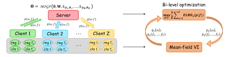
Figure 1. The overview of our model pFed-Mul. Left: System diagram. The central server aggregates the posteriors from local devices, updating a global MOGP prior redistributed for training local models. Right: Bi-level optimization. The subfigure illustrates an iterative application of mean-field VI at the local level and hyperparameter tuning at the global level.

The overview of our model pFed-Mul. Left: System diagram. The central server aggregates the posteriors from local devices, updating a global MOGP prior redistributed for training local models. Right: Bi-level optimization. The subfigure illustrates an iterative application of mean-field VI at the local level and hyperparameter tuning at the global level.

In a distributed system comprising a single server and $\mathcal{Z}$ clients, where each client manages multiple correlated regression and classification tasks. For convenience, we assume an identical dataset size across all clients. On each client, we assume there are $T_{r}$ regression tasks with data $\mathcal{D}^{r}=\{{(\mathbf{x}_{i,n}^{r},y_{i,n}^{r})}_{n=1}^{N_{i}^{r}}\}_{i=1}^{T_{r}}$ and $T_{c}$ classification tasks with data $\mathcal{D}^{c}=\{{(\mathbf{x}_{i,n}^{c},y_{i,n}^{c})}_{n=1}^{N_{i}^{c}}\}_{i=1}^{T_{c}}$. $\mathbf{x}\in\mathcal{X}\subset\mathbb{R}^{D}$ represents the $D$-dim input. In regression, the output $y\in\mathbb{R}$, while in classification $y\in\{-1,1\}$.

4.1. Client Level

We present a MOGP-based multi-task learning model deployed on each client and detail optimization of the posterior distributions of latent functions.

4.1.1. MOGP Model

The correlation between classification and regression tasks is characterized by the MOGP prior and can be utilized to transfer knowledge, especially in scenarios with limited data (Moreno-Muñoz et al., 2018). Therefore, we obtain the Bayesian multi-task learning model based on MOGP on each client:

(1a) $$\mathbf{y}^{r}\mid\{f_{i}^{r}\}_{i=1}^{T_{r}}\sim\prod_{i=1}^{T_{r}}\prod_{n=1}^{N_{i}^{r}}\mathcal{N}(f^{r}_{i,n},\sigma_{i}^{2}),$$

(1b) $$\mathbf{y}^{c}\mid\{f_{i}^{c}\}_{i=1}^{T_{c}}\sim\prod_{i=1}^{T_{c}}\prod_{n=1}^{N^{c}_{i}}\mathcal{B}(s(y^{c}_{i,n}f^{c}_{i,n})),$$

(1c) $$f_{1},\ldots,f_{T}\sim\mathcal{MOGP}(0,\mathbf{W},k_{1},\ldots,k_{B}),$$

where Equation˜1a is the regression likelihood, Equation˜1b is the classification likelihood, and Equation˜1c is the MOGP prior; $f_{i}^{r}$ and $f_{i}^{c}$ refer to the respective $i$-th output function for the $T_{r}$ regression and $T_{c}$ classification tasks, $f_{1},\ldots,f_{T}$ represent organizing all regression and classification functions together, thus $T=T_{r}+T_{c}$; $f^{\cdot}_{i,n}=f^{\cdot}_{i}(\mathbf{x}^{\cdot}_{i,n})$, $\mathbf{y}^{r}$ denotes all regression targets, $\mathbf{y}^{c}$ denotes all classification labels, $\mathbf{W}$ is the matrix of all mixing weights $w_{i,b}$, and $k_{1},\ldots,k_{B}$ correspond to the kernels of $B$ basis functions. It is worth noting that we use logistic regression for classification tasks, meaning that the link function $s(\cdot)$ in Equation˜1b is sigmoid. This choice facilitates the use of Pólya-Gamma augmentation, simplifying the inference process afterward.

4.1.2. Posterior of Latent Functions

Given the model provided in Equation˜1, the remaining task is to infer the posterior of each output function. For inference, as discussed in Section˜3.1, the likelihood of classification tasks is not conjugate to the prior, resulting in non-analytical posteriors for $f_{1},\ldots,f_{T}$. To address the non-conjugacy issue, many existing works employed Gaussian variational inference (Hensman et al., 2015; Jahani et al., 2021). This method assumes the variational distribution to be Gaussian, making the ELBO tractable. However, this method has drawbacks. On the one hand, it relies on parametric assumptions for the variational distribution, leading to increased approximation errors, especially when the true posterior deviates from Gaussian. On the other hand, due to the need to compute the expected log-likelihood in ELBO, which often requires Monte Carlo approximation, it typically exhibits low computational efficiency.

To address the above issue, we adapt the Pólya-Gamma augmentation for MOGP to the federated setting. We augment the MOGP model with Pólya-Gamma random variables $\bm{\omega}$ for all classification tasks, one for each sample. Consequently, the original non-conjugate model $p(\mathbf{y}^{r},\mathbf{y}^{c},f_{1},\ldots,f_{T})$ is augmented to be a conditionally conjugate model $p(\mathbf{y}^{r},\mathbf{y}^{c},\bm{\omega},f_{1},\ldots,f_{T})$ allowing us to derive an analytical mean-field VI method. Following the common practice of mean-field VI, we approximate the true posterior in a factorized manner: $p(\bm{\omega},f_{1},\ldots,f_{T}\mid\mathbf{y}^{r},\mathbf{y}^{c})\approx q(\bm{\omega},f_{1},\ldots,f_{T})=q_{1}(\bm{\omega})q_{2}(f_{1},\ldots,f_{T})$. The optimal variational distribution is obtained by minimizing the Kullback-Leibler (KL) divergence between the factorized variational distribution and the true posterior, which is equivalent to the following optimization of ELBO:

(2) $$\max_{q(\bm{\omega},f)}\bigg{\{} \mathbb{E}_{q(\bm{\omega},f)}[\log p(\mathbf{y}^{r},\mathbf{y}^{c}\mid\bm{\omega},\{f_{i}^{r}\}_{i=1}^{T_{r}}),\{f_{i}^{c}\}_{i=1}^{T_{c}})]$$

$$-\text{KL}(q(\bm{\omega},f)\|p(\bm{\omega},f))\bigg{\}}.$$

where $p(\omega,f)$ is the prior distribution distributed from server and fixed during local update. Specifically, the prior distribution is assumed as $p(\omega,f)=p(\omega)p(f)$ where $p(\omega)=p_{\text{PG}}(1,0)$ and $p(f)=\mathcal{MOGP}(0,\mathbf{W},k_{1},\cdots,k_{B})$. Under assumption of factorized variational distribution, we obtain the following local updates:

(3a) $$q_{1}(\bm{\omega})=\prod_{i=1}^{T_{c}}\prod_{n=1}^{N_{i}^{c}}p_{\text{PG}}(\omega_{i,n}\mid 1,\tilde{f}_{i,n}^{c}),$$

(3b) $$q_{2}(\mathbf{f})=\mathcal{N}(\mathbf{m},\mathbf{\Sigma}),$$

where $\tilde{f}_{i,n}^{c}=\sqrt{\mathbb{E}[f_{i,n}^{c^{2}}]}$, $\mathbf{\Sigma}=(\mathbf{H}+\mathbf{K}^{-1})^{-1}$, $\mathbf{m}=\mathbf{\Sigma}\mathbf{H}\mathbf{v}$,with $\mathbf{H}=\text{diag}(\mathbf{D}^{r}_{\cdot},\mathbf{D}^{c}_{\cdot})$, $\mathbf{v}=[\mathbf{y}^{r}_{\cdot},\frac{1}{2}{\mathbf{D}^{c}_{\cdot}}^{-1}\mathbf{y}^{c}_{\cdot}]^{\top}$, and $\mathbf{D}^{r}_{i}=\text{diag}(1/\sigma_{i}^{2})$, $\mathbf{D}^{c}_{i}=\text{diag}(\mathbb{E}[\bm{\omega}_{i}])$. The detailed derivation of Pólya-Gamma augmentation and mean-field VI is provided in Appendices˜A and B.

After obtaining the posterior distribution of $\mathbf{f}$, we can calculate the analytical expression for the predictive distribution at any point:

(4) $$q(f_{i}(x)) =\int p(f_{i}(x)\mid\mathbf{f}^{i})q_{2}(\mathbf{f}^{i})d\mathbf{f}^{i}=\mathcal{N}(\mu,\sigma^{2}),$$

$$\mu =\mathbf{k}_{\mathbf{x}^{\cdot}_{i}x}^{\top}\mathbf{K}_{\mathbf{x}^{\cdot}_{i}\mathbf{x}^{\cdot}_{i}}^{-1}\mathbf{m}_{\mathbf{x}_{i}^{\cdot}},$$

$$\sigma^{2} =k_{xx}-\mathbf{k}_{\mathbf{x}_{i}^{\cdot}x}^{\top}\mathbf{K}_{\mathbf{x}^{\cdot}_{i}\mathbf{x}^{\cdot}_{i}}^{-1}\mathbf{k}_{\mathbf{x}^{\cdot}_{i}x}+\mathbf{k}_{\mathbf{x}^{\cdot}_{i}x}^{\top}\mathbf{K}_{\mathbf{x}^{\cdot}_{i}\mathbf{x}^{\cdot}_{i}}^{-1}\mathbf{\Sigma}_{\mathbf{x}^{\cdot}_{i}}\mathbf{K}_{\mathbf{x}^{\cdot}_{i}\mathbf{x}^{\cdot}_{i}}^{-1}\mathbf{k}_{\mathbf{x}_{i}x}.$$

4.2. Server Level

The server maintains a global MOGP prior for the entire system, aggregates local posteriors to update the global MOGP prior, and distributes the updated global prior back to clients. The intuition behind our method is similar to that of pFedBayes (Zhang et al., 2022). In practice, we often cannot directly assume a good prior suitable for the current data. As the communication rounds progress, the global MOGP becomes increasingly compatible with the data from all clients. This implies that we have found a relatively good prior. pFedBayes is a parametric method that assumes Gaussian variational distributions for each parameter, an assumption that may not always hold true. In contrast, our proposed method is non-parametric and imposes no assumptions on the form of the posterior distribution, with the only restriction being the independence between $f$ and $\bm{\omega}$.

Specifically, at the server level, we aggregate the mean-field VI posteriors uploaded from clients and update the global MOGP prior by maximizing the averaged ELBO:

(5) $$\max_{p(f)}\frac{1}{\mathcal{Z}}\sum_{z=1}^{\mathcal{Z}}\text{ELBO}_{z}(p(f)),$$

where $\text{ELBO}_{z}$ represents the ELBO of the $z$-th client, which depends on the variational distribution $q$ and prior $p$. Since $q$ is uploaded by the client and fixed, the ELBO is solely a function of $p$. Thanks to the Pólya-Gamma augmentation, Equation˜5 has an analytical solution, thus we can optimize the parameters of the prior, i.e., the kernel hyperparameters $\{\bm{\phi}_{b}\}_{b=1}^{B}$ pertain to B basis functions, the mixing weight $\mathbf{W}$, and the regression noise variance $\{\sigma_{i}^{2}\}_{i=1}^{T_{r}}$. The detailed derivation of Equation˜5 is provided in Appendix˜D.

For new incoming clients, based on the global MOGP served as a shared prior, the posterior of the classification and regression functions is further inferred with incorporation of their local data, which ensures personalization at the client level.

4.3. Deep Kernel and Inducing Points

To further enhance the expressive capacity of MOGP, a deep kernel (Wilson et al., 2016) is utilized in this study. The deep kernel involves a neural network $\eta(\cdot)$ with parameters $\bm{\theta}$ that transforms input data $x$ into a latent representation $\eta_{\bm{\theta}}(x)$. Subsequently, this representation is fed into a traditional kernel, thereby generating a new kernel:

$$k_{\bm{\phi},\bm{\theta}}(x_{1},x_{2})=\tilde{k}_{\bm{\phi}}(\eta_{\bm{\theta}}(x_{1}),\eta_{\bm{\theta}}(x_{2})),$$

where $\tilde{k}_{\bm{\phi}}(\cdot,\cdot)$ is the base kernel, e.g., the radial basis function (RBF) kernel or others. One advantage of the deep kernel is its ability to learn a flexible input transformation metric in a data-driven manner, instead of relying directly on Euclidean distance based metrics that might not be suitable. For MOGP, $k_{1},\ldots,k_{B}$ in Equation˜1c are modeled by deep kernels. Consequently, our model hyperparameters of prior $\bm{\Theta}$ include the kernel hyperparameters $\{\bm{\phi}_{b},\bm{\theta}_{b}\}_{b=1}^{B}$, the mixing weight $\mathbf{W}$, and the regression noise variance $\{\sigma_{i}^{2}\}_{i=1}^{T_{r}}$. These hyperparameters are updated by maximizing averaged ELBO uploaded from each clients without alteration of the analytical solution in Equation˜5.

MOGP inherits GP’s notorious cubic computational complexity w.r.t. the number of samples. The complexity of $O(N^{3})$ becomes intolerable as the sample size $N$ per client increases. To enhance the computational efficiency, we employ the inducing points method (Titsias, 2009). We assume that these inducing inputs on each client are uniformly sampled from local data and not uploaded to the server for aggregation, which upholds local privacy. After introducing $M$ inducing points, the computational complexity decreases to $O(NM^{2})$ ($M\ll N$), which is linear w.r.t. the number of samples on each client. The detailed derivation of mean-field VI with inducing points is provided in Appendix˜C.

Algorithm 1 pFed-Mul: Server

 Input: server iteration $\mathcal{T}_{s}$, client size $\mathcal{Z}$, sample size $\mathcal{S}$ and initial global hyperparameters $\bm{\Theta}^{(g)}$,

 for $t_{s}=0$ to $\mathcal{T}_{s}-1$ do

  $\mathbb{S}_{t_{s}}$ $\leftarrow$ Sample randomly the subset of clients with size $\mathcal{S}$

  for each client $z$ in $\mathbb{S}_{t_{s}}$ do

   $\bm{\Theta}_{z}^{(l)}$ $\leftarrow$ Sent global hyperparameters $\bm{\Theta}^{(g)}$ to client $z$,

   $q_{z,1}(\bm{\omega})$, $q_{z,2}(\mathbf{f})$ $\leftarrow$ Update local posteriors based on specific client data by Algorithm˜2,

  end for

  $\bm{\Theta}^{(g)}$ $\leftarrow$ Optimize global MOGP prior according to Equation˜5.

 end for

Algorithm 2 pFed-Mul: Client

 Input: client iteration $\mathcal{T}_{c}$, initial local hyperparameters $\bm{\Theta}_{z}^{(l)}$ for client $z$,

 for $t_{c}=0$ to $\mathcal{T}_{c}-1$ do

  $q_{1}(\bm{\omega})$ $\leftarrow$ Update variational distribution of Pólya-Gamma variables by Equation˜3a,

  $q_{2}(\mathbf{f})$ $\leftarrow$ Update variational distribution of latent functions by Equation˜3b,

 end for

 $q(f(x))\leftarrow$ Compute the predictive distribution of test points according to Equation˜4,

4.4. Algorithm

In summary, at the client level, all clients receive the same global prior distributed by server, alternately update variational distributions $q(\bm{\omega})$ and $q(f)$ via Equation˜3 to approximate posterior distributions based on the local data. At the server level, variational distributions $q(\bm{\omega})$ and $q(f)$ are aggregated and the averaged ELBO is optimized to update the glocal MOGP prior via Equation˜5. We term our method pFed-Mul whose pseudocode is provided in Algorithms˜1 and 2.

5. Experiments

In this section, we utilize a synthetic dataset and two real-world datasets to showcase the performance of pFed-Mul in terms of accuracy, uncertainty estimation, and convergence. We did all experiments in this paper using servers with two GPUs (NVIDIA TITAN V with 12GB memory), two CPUs (each with 8 cores, Intel(R) Xeon(R) CPU E5-2620 v4 @ 2.10GHz), and 251GB memory.

5.1. Experimental Setup

5.1.1. Datasets

We consider three datasets, including one synthetic dataset and two image datasets.

Synthetic Data: we assume that there exists 5 clients and each has one regression task and one classification task. The regression function $f_{r}$ and the classification function $f_{c}$ are assumed to be sampled from a MOGP on the domain $[0,100]$ with two kernels: $f_{r},f_{c}\sim\mathcal{MOGP}(0,\mathbf{W},k_{1},k_{2})$. We select the RBF kernel $k(x_{1},x_{2})=\phi_{0}\exp(-\frac{\phi_{1}}{2}\|x_{1}-x_{2}\|_{2}^{2})$. The regression function $f_{r}$ is used in Equation˜1a with a fixed noise variance $\sigma^{2}$ to sample the regression targets $\mathbf{y}_{r}$. The classification function $f_{c}$ is used in Equation˜1b to sample the classification labels $\mathbf{y}^{c}$. We simulate the synthetic data, where hyperparameters are $\sigma^{2}=0.1$, $\mathbf{W}=[[0.6,0.4],[0.4,0.6]]$, $\phi_{0}^{(1)}=1,\phi_{0}^{(2)}=2$, $\phi_{1}^{(1)}=0.02,\phi_{1}^{(2)}=0.01$.

CelebA: this dataset comprises an extensive collection of over two million face images of celebrities, each accompanied by forty attribute annotations. The dataset exhibits a diverse range of images featuring significant variations in poses and background settings. Each image is associated with regression targets, such as the position of eyes, mouth, and classification labels such as the presence of eyeglasses, hair color, and smiling expressions. For more comprehensive details, readers are encouraged to refer to (Liu et al., 2015). In our study, we specifically select the abscissa of the right side of the mouth as regression labels and whether or not the subject is smiling as classification labels. Given the close relationship between the position of the mouth corner and smiling, these two types of tasks have the potential to mutually transfer knowledge.

Dogcat: this dataset includes $20,000$ genuine images of dogs and cats and is widely employed for binary classification tasks in computer vision. The images in the dataset showcase various breeds of dogs and cats, captured in different poses, backgrounds, and lighting conditions. The primary objective of the dataset is to identify whether the images contain a dog or a cat, without the inclusion of regression labels. To create new regression labels, we introduce zero-mean Gaussian noise with a variance of $0.5$ into the original classification labels. As a result, regression labels exhibit bi-modal distribution. Specifically, for dog images, the regression targets are centered around $1$, while for cat images, they are centered around $-1$. It is evident that the classification labels and regression targets are closely related.

Table 1. The mean square error (MSE) for regression tasks and prediction accuracy (ACC) for classification tasks for all models. The experiments are conducted for two datasets, CelebA and Dogcat, under three few-shot scenarios, 10-shot 20-client, 20-shot 15-client, and 50-shot 10-client. FedPAC, pFedGP and pFedVEM are originally designed to process only the classification tasks, hence their results for regression tasks are not reported. The champion is highlighted in bold, runner-up with underline. ✗indicates the model cannot handle this type of tasks.

The mean square error (MSE) for regression tasks and prediction accuracy (ACC) for classification tasks for all models. The experiments are conducted for two datasets, CelebA and Dogcat, under three few-shot scenarios, 10-shot 20-client, 20-shot 15-client, and 50-shot 10-client. FedPAC, pFedGP and pFedVEM are originally designed to process only the classification tasks, hence their results for regression tasks are not reported. The champion is highlighted in bold, runner-up with underline. ✗indicates the model cannot handle this type of tasks. CelebA Dogcat 10-shot 20-client 20-shot 15-client 50-shot 10-client 10-shot 20-client 20-shot 15-client 50-shot 10-client MSE($\downarrow$) ACC%($\uparrow$) MSE($\downarrow$) ACC%($\uparrow$) MSE($\downarrow$) ACC%($\uparrow$) MSE($\downarrow$) ACC%($\uparrow$) MSE($\downarrow$) ACC%($\uparrow$) MSE($\downarrow$) ACC%($\uparrow$) FedAvg 0.672 82.50 0.514 86.33 0.394 89.59 0.667 94.70 0.576 94.63 0.515 97.13 FedPer 0.369 79.04 0.328 81.37 0.261 86.68 0.731 95.40 0.682 96.92 0.512 97.13 Scaffold 0.774 77.36 0.649 79.32 0.545 85.12 0.720 94.41 0.667 96.77 0.541 97.43 pFedMe 0.792 78.04 0.657 79.84 0.552 85.44 0.751 94.60 0.673 96.82 0.543 97.13 FedPAC ✗ 77.81 ✗ 79.17 ✗ 81.60 ✗ 96.72 ✗ 97.51 ✗ 97.96 pfedGP ✗ 76.96 ✗ 87.95 ✗ 89.92 ✗ 92.67 ✗ 97.41 ✗ 98.17 pFedVEM ✗ 78.91 ✗ 80.47 ✗ 84.12 ✗ 95.03 ✗ 95.55 ✗ 97.32 pFed-St 0.690 83.80 0.321 88.31 0.221 90.28 0.799 96.83 0.570 96.92 0.525 97.82 pFed-Mul 0.488 86.36 0.476 88.47 0.301 90.76 0.512 96.88 0.422 97.46 0.398 98.22

5.1.2. Baselines

We compare our pFed-Mul with competitive FL methods, which can be categorized into two groups: (1) Bayesian FL methods, pFedGP (Achituve et al., 2021) and pFedVEM (Zhu et al., 2023); (2) frequentist FL methods, FedAvg (McMahan et al., 2017), FedPer (Arivazhagan et al., 2019), Scaffold (Karimireddy et al., 2020), pFedMe (T Dinh et al., 2020) and FedPAC (Xu et al., 2023). As the existing methods are designed for single task, we implement them separately for each type of task and present the respective outcomes. Moreover, we introduce an additional single-task version of pFed-Mul, denoted as pFed-St, which is exclusively designed to handle a single type of tasks.

5.1.3. Training Protocol

For the synthetic dataset, at the server level, we assume a global MOGP prior with two RBF kernels without deep architecture and distribute it to each client. At the client level, posterior distributions are updated via mean-field VI and sent back to the server for optimizing the averaged ELBO w.r.t. hyperparameters $\mathbf{W}$, $\bm{\phi}$, and $\sigma^{2}$. We initialize all hyperparameters as the ground truth. The number of global communication rounds, mean-field iterations and local updates are set to 20, 2 and 2, respectively.

Similarly, for the real-world datasets, we assume that each client has one regression task and one classification task. The training data are partitioned in a non-overlapping manner and distributed to individual clients. It is worth noting that this setup is designed for computational convenience, but our method can adapt to scenarios involving multiple tasks (more than two) per client and task heterogeneity among clients. A MOGP prior with two deep kernels is employed where RBF serves as the base kernel. The deep architecture $\eta_{\bm{\theta}}(\cdot)$ in the deep kernel is implemented using ResNet-18 (He et al., 2016). The initial hyperparameters are set as follows, $\phi_{0}^{(1)}=\phi_{0}^{(2)}=1,\phi_{1}^{(1)}=\phi_{1}^{(2)}=0.01,\sigma^{2}=0.1$, and $\mathbf{W}$ is tuned with fixed other hyperparameters. The number of global communication rounds, mean-field iterations and local updates are set to 70, 2 and 2, respectively. To demonstrate the advantage of our model, all real-world data experiments are conducted in few-shot settings where each client possesses only limited data.

Furthermore, we have the option to update global MOGP prior by optimizing summation of ELBOs from a selection of clients according to Equation˜5. Alternatively, we can update certain hyperparameters by Equation˜5, while retaining others that are optimized by client specific ELBOs. This strategy is designed to improve the level of personalization for the clients. Specifically, we update all hyperparamters $\mathbf{W}$, $\bm{\phi}$, $\sigma^{2}$ of global prior for synthetic dataset via Equation˜5, while solely backbone $\bm{\theta}$ for real image datasets with others optimized locally.

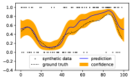
(a) pFed-Mul (left:regression right:classification)

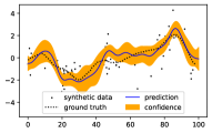
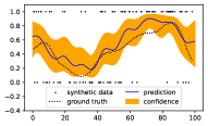
(b) pFed-St (left:regression right:classification)

Figure 2. The estimated posterior of latent functions from pFed-Mul and pFed-St on one client. pFed-Mul, achieves a better fit, especially for classification. Compared with pFed-St, pFed-Mul enables the transfer of knowledge from other task types, effectively reducing uncertainty, i.e. posterior variance (orange areas).

The estimated posterior of latent functions from pFed-Mul and pFed-St on one client. pFed-Mul, achieves a better fit, especially for classification. Compared with pFed-St, pFed-Mul enables the transfer of knowledge from other task types, effectively reducing uncertainty, i.e. posterior variance (orange areas).

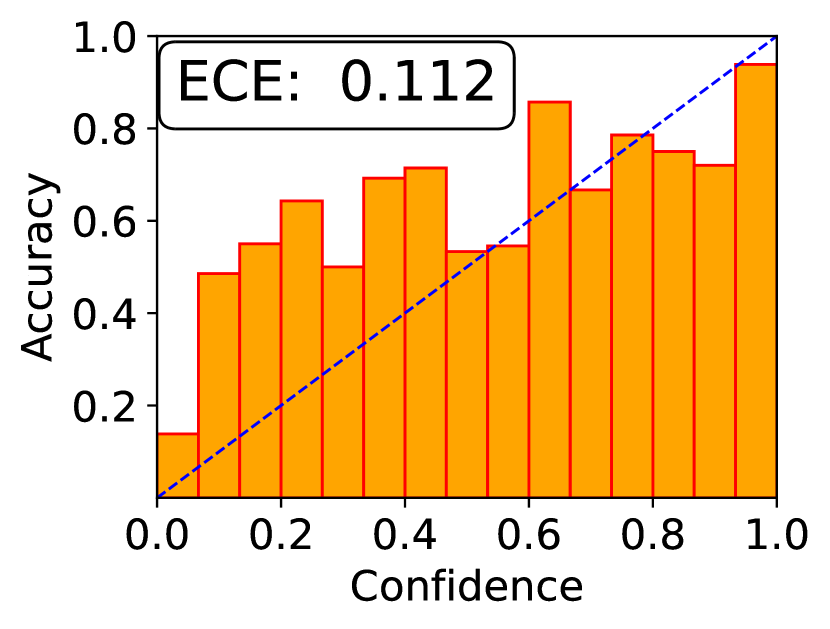
(a) FedAvg

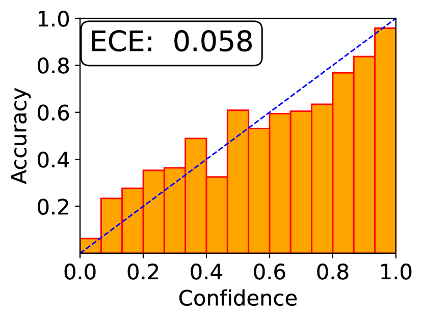
(b) FedPer

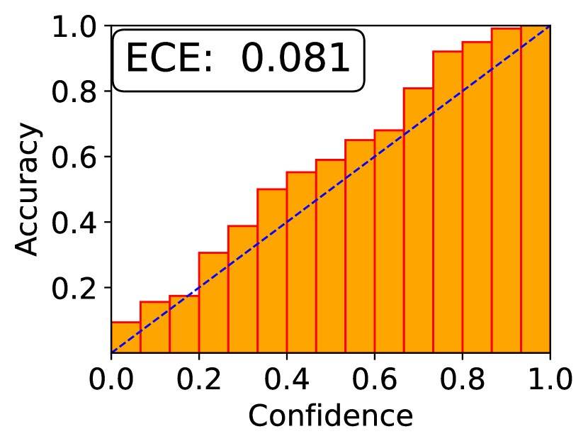
(c) Scaffold

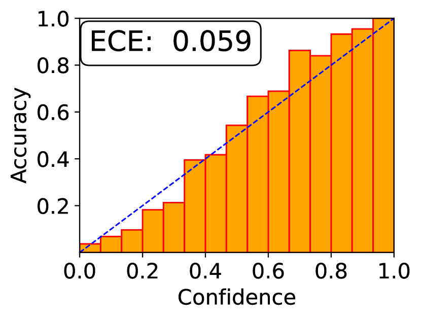
(d) pFedMe

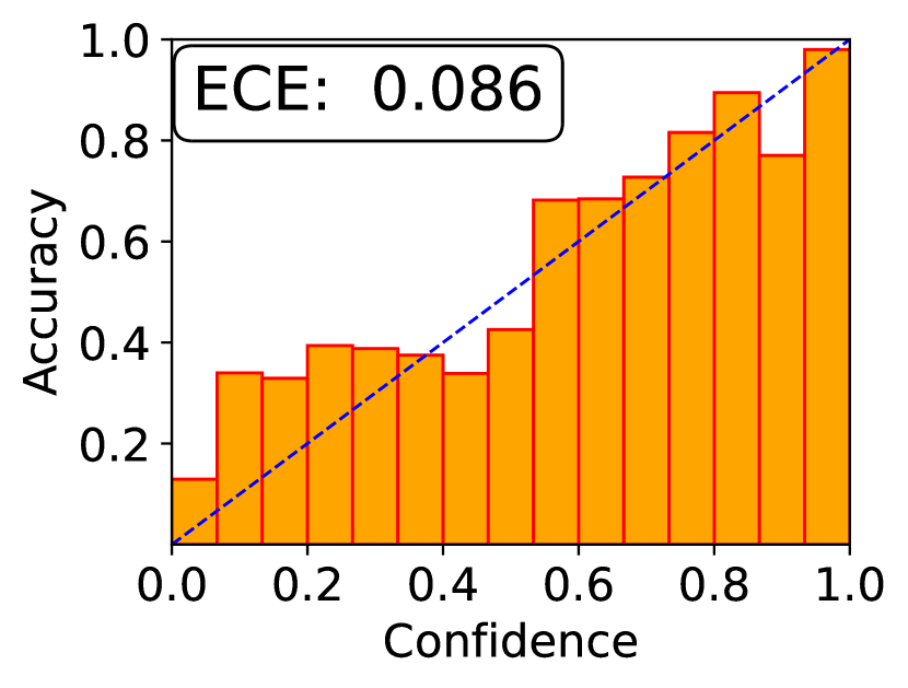
(e) FedPAC

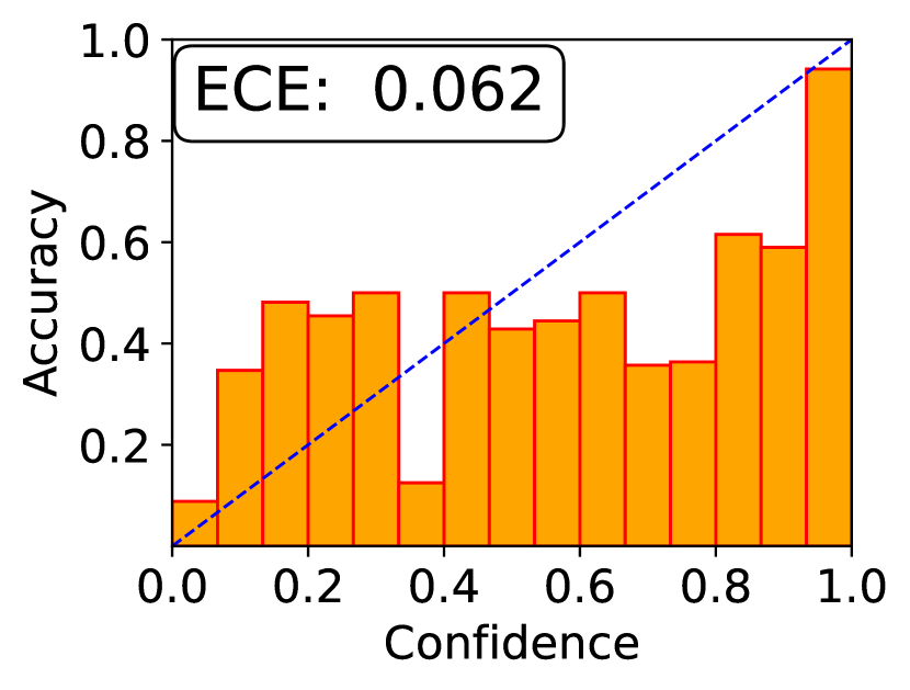
(f) pFedGP

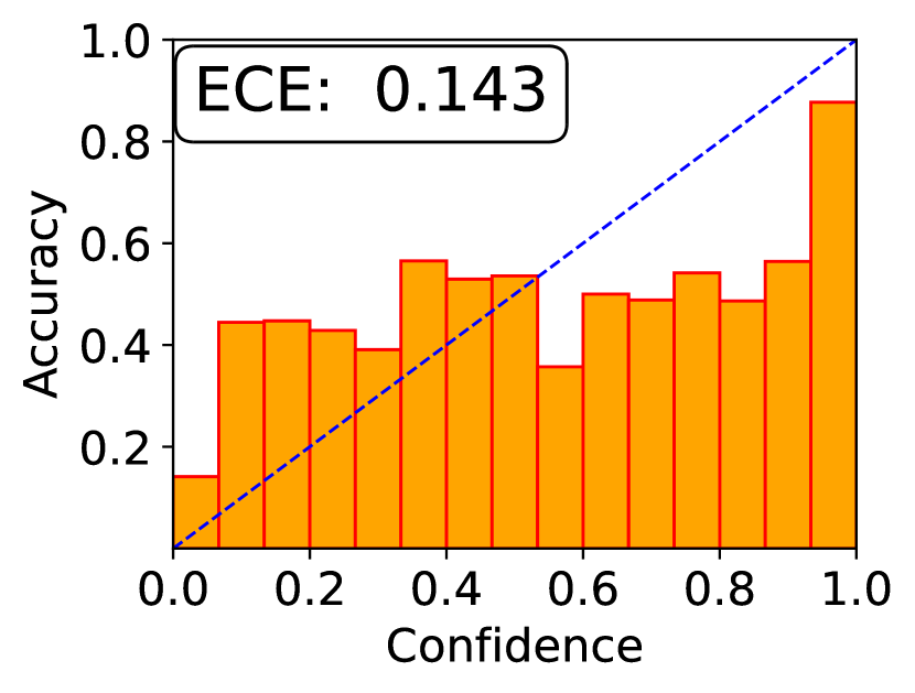
(g) pFedVEM

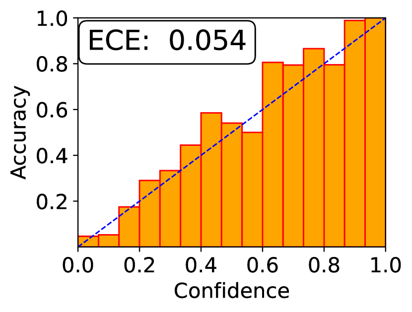
(h) pFed-Mul

Figure 3. Reliability diagrams for all methods. We plot the perfect calibration as blue diagonals, and practical result as orange bars. The disparity between the top of orange bars and blue line represents the degree of calibration, with the expected calibration error (ECE) calculated for comparison and placed in the top-left corner of diagrams. Our proposed method, pFed-Mul, demonstrates best calibration performance, ranking first in terms of ECE.

Reliability diagrams for all methods. We plot the perfect calibration as blue diagonals, and practical result as orange bars. The disparity between the top of orange bars and blue line represents the degree of calibration, with the expected calibration error (ECE) calculated for comparison and placed in the top-left corner of diagrams. Our proposed method, pFed-Mul, demonstrates best calibration performance, ranking first in terms of ECE.

5.2. Performance of Prediction

5.2.1. Synthetic Data

We conduct a visual analysis to compare the estimated posterior of latent functions from pFed-Mul with that from pFed-St on one client in Figure˜2.

As shown in Figure˜2(a), the results indicate that our proposed method successfully recovers the ground-truth latent functions. Furthermore, by comparing pFed-Mul to pFed-St (Figure˜2(b)) that handle only one type of tasks, we summarize key findings as follows. (1) We observe that pFed-Mul improves the fitting of latent functions, especially for the classification functions. The more significant improvement for the classification functions can be attributed to the fact that the target values of regression functions exhibit greater volatility, making them relatively easier to estimate. Conversely, the target values of classification functions, passed through a sigmoid function, are compressed within the range of $[0,1]$, thereby making their estimation more challenging. (2) For pFed-St, a smaller data size results in greater uncertainty in parameter estimation (posterior variance), while pFed-Mul facilitates knowledge transfer across different task types, thereby reducing such uncertainty. These outcomes show the necessity of knowledge transfer among diverse task types, particularly in few-shot scenarios.

5.2.2. Real Data

We conduct experiments on CelebA and Dogcat, in three different settings: 10-shot individually among 20 clients, 20-shot individually among 15 clients, and 50-shot individually among 10 clients. The evaluation metrics including mean square error (MSE) for regression tasks and prediction accuracy (ACC) for classification tasks are computed for all methods.

The results, summarized in Table˜1, show that, (1) pFed-Mul consistently outperforms existing methods across almost all scenarios. This observation showcases remarkable adaptability of our proposed method from synthetic datasets to intricate real datasets. In terms of evaluation metrics, the most significant improvements observed in regression and classification tasks amount to $0.155$ and $3.86\%$ respectively. (2) In comparison to the single-task baseline models, the utilization of the multi-task framework demonstrates an increase of accuracy in both regression and classification tasks, highlighting the advantage of multi-task learning, particularly with limited data. This success can be attributed to two aspects. Firstly, incorporating more tasks enables the utilization of additional data, mitigating local overfitting and enhancing global robustness. Secondly, leveraging prior knowledge among tasks achieves better prior distribution and enhances convergence efficiency.

5.3. Performance of Uncertainty Estimation

We illustrate that our method can qualify uncertainty and achieve superior performance to previous baselines in terms of model calibration and OOD detection. These evaluations are conducted in a setting of $50$-shot individually among $10$ clients.

5.3.1. Model Calibration

We assess uncertainty by calibrating the binary classification tasks for CelebA. The reliability diagrams, as depicted in Figure˜3, showcase the disparity between the perfect calibration (blue diagonals) and the model’s calibration (orange bars). To quantitatively compare the calibration, we calculate the expected calibration error (ECE), which measures weighted average between empirical accuracy and model’s confidence as suggested in (Guo et al., 2017). The results indicate that pFed-Mul demonstrates calibration performance superior to the baseline models. Specifically, pFed-Mul ranks first in terms of ECE, FedPer exhibits runner-up performance, and pFedVEM performs worst among all baselines.

5.3.2. OOD Detection

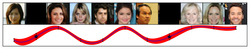
(a) CelebA

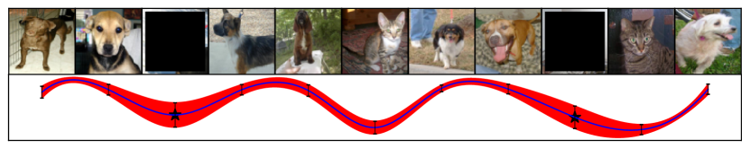
(b) Dogcat

Figure 4. OOD detection for CelebA and Dogcat. The predictive mean and variance of latent functions are depicted by blue lines and red areas beneath each image respectively. Positions where the image is masked as an OOD sample are denoted by black stars. A greater variance (wider area) is observed for OOD samples.

OOD detection for CelebA and Dogcat. The predictive mean and variance of latent functions are depicted by blue lines and red areas beneath each image respectively. Positions where the image is masked as an OOD sample are denoted by black stars. A greater variance (wider area) is observed for OOD samples.

The uncertainty of prediction provided by the Bayesian framework is crucial for detecting OOD samples. To demonstrate this, we select a series of samples from CelebA and Dogcat, randomly mask two of them, and compute the predictive variance in classification tasks. The results are depicted in Figure˜4(b). It is evident that the masked images demonstrate a larger semantic shift compared to in-distribution images. Therefore, we observe a greater predictive variance (depicted as red areas) under them. This visualization highlights the robustness of our method: pFed-Mul not only provides predictions but also outputs the uncertainty of predictions. When the uncertainty is large, it indicates that the model is not confident in the predicted results.

5.4. Convergence Rate

We conduct a comparison between pFed-Mul and other baselines about convergence rate. For all models, in each communication round, we assume that the local parameters/variational distributions are updated $2$ times before being uploaded to the server in a setting of 50-shot individually among 10 clients. The convergence curve of test accuracy for classification tasks within the initial $10$ communication rounds is depicted in Figure˜5(b).

In Figure˜5(a), pFed-Mul consistently converges to the best test accuracy plateau after 10 global rounds of communication, with a remarkable convergence rate. Meanwhile, in Figure˜5(b), pFed-Mul not only outperforms other methods in the initial rounds, showing a substantial lead over the runner-up, pFedGP, but also maintains stable performance comparable to other approaches. The superior convergence rate of pFed-Mul stems from our adoption of Pólya-Gamma augmentation for classification tasks. As proven in (Hoffman et al., 2013), employing mean-field VI for a conditionally conjugate model is equivalent to optimizing the ELBO using natural gradient descent (Amari, 1998) with step size of $1$. This second-order optimization method exhibits an improved convergence rate compared to traditional first-order optimization methods.

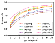
(a) CelebA

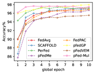
(b) Dogcat

Figure 5. Convergence rate of all models on both datasets. pFed-Mul consistently converges to a comparable test accuracy plateau with a remarkable convergence rate.

Convergence rate of all models on both datasets. pFed-Mul consistently converges to a comparable test accuracy plateau with a remarkable convergence rate.

Beyond the convergence rate, the test accuracy convergence curve of pFed-Mul exhibits a stable monotonic increase without significant fluctuations, indicating remarkable stability. Both convergence rate and stability, hold paramount importance for a model’s adaptability in real-world scenarios, emphasizing training efficiency, low latency, and remarkable performance.

5.5. Ablation Studies

We conduct ablation studies to assess various model components in the setting of 50-shot individually among 10 clients, enhancing our comprehension of the model’s behavior.

Aggregated Hyperparameters

In the implementation, we can optimize only specific hyperparameters by Equation˜5, leaving the rest optimized by local ELBOs, thereby enhancing personalization for the clients. To investigate this, we compare several versions of pFed-Mul: pFed-Mul-N which optimizes the parameters of the neural network in the deep kernel $\bm{\theta}$ on server (the one we use in Section˜5.2); pFed-Mul-K which optimizes all kernel hyperparameters $\bm{\phi},\bm{\theta}$ on server; pFed-Mul-W which optimizes all kernel hyperparameters and mixing weights $\bm{\phi},\bm{\theta},\mathbf{W}$ on server; pFed-Mul-A which optimizes all hyperparameters $\bm{\phi},\bm{\theta},\mathbf{W},\sigma^{2}$ on server. The results are shown in Table˜2. We can see that pFed-Mul-N strikes a balance between local personalization and global generalization, outperforming other versions. pFed-Mul-A performs unsatisfying, underscoring the necessity of personalization in FL.

Table 2. The prediction performance for ablation studies. In the first block, we analyze different levels of personalization with various optimized hyperparameters. In the second block, we conduct experiments with different base kernels. In the third block, we compare different backbones.

The prediction performance for ablation studies. In the first block, we analyze different levels of personalization with various optimized hyperparameters. In the second block, we conduct experiments with different base kernels. In the third block, we compare different backbones. CelebA Dogcat MSE($\downarrow$) ACC%($\uparrow$) MSE($\downarrow$) ACC%($\uparrow$) Aggregated Hyperparameters pFed-Mul-K 0.313 88.56 0.659 98.12 pFed-Mul-W 0.449 88.04 0.426 97.82 pFed-Mul-A 0.466 87.52 0.417 97.92 pFed-Mul-N 0.301 90.76 0.398 98.22 Base Kernel Linear Kernel 0.476 85.80 0.442 96.98 Laplace Kernel 0.436 90.36 0.485 97.87 Cauchy Kernel 0.385 90.40 0.453 97.87 RBF Kernel 0.301 90.76 0.398 98.22 Backbone EfficientNet 0.306 89.64 0.405 97.67 ShuffleNet 0.396 87.44 0.421 96.09 RegNet 0.301 89.00 0.409 98.22 ResNet 0.301 90.76 0.398 98.22

Base Kernel

The base kernels in MOGP also have a significant impact on the results. We compare the MOGP models with linear kernel, Laplace kernel, Cauchy kernel, and RBF kernel. The expressions for all kernels are shown in Appendix˜F. The results are shown in Table˜2, and reveal that the RBF kernel stands out as the best-performing kernel, consistent with previous studies. Additionally, the Cauchy kernel achieves a runner-up position, demonstrating results comparable to the RBF kernel. In contrast, the linear kernel exhibits inferior performance.

Backbone

Recalling that we employ ResNet-18 as the backbone in deep kernels, it is necessary to analyse the impact of backbone on the prediction performance. Therefore, we replace ResNet-18 with EfficientNet-B2 (Tan and Le, 2019), ShuffleNet-v2-2x (Ma et al., 2018), RegNet-Y-1.6GF (Radosavovic et al., 2020) and report results on both dataset in Table˜2, where the amounts of parameters of all backbones are comparable. The results demonstrate that it is beneficial for prediction to utilize ResNet-18 as the feature extractor. Meanwhile, ShuffleNet exhibits worst performance among all backbones.

6. Conclusion

In summary, our approach addresses a crucial limitation in FL, considering task diversity on clients. The proposed approach integrates multi-task learning using MOGP at the local level and federated learning at the global level. MOGP is effective in handling correlated classification and regression tasks, providing a Bayesian non-parametric framework that inherently quantifies uncertainty. To overcome challenges in posterior inference, we employ the Pólya-Gamma augmentation technique, leading to an analytical mean-field VI. The experimental results demonstrate our method’s superiority in predictive performance, uncertainty calibration, OOD detection and convergence rate. The results highlight the method’s potential across diverse applications.

Appendix A Classification Likelihood with Pólya-Gamma Augmentation

Proof.

In accordance with Theorem 1 in (Polson et al., 2013), the likelihood of classification task is delineated as follows,

$$p(\mathbf{y}_{i}^{c}\mid\mathbf{f}_{i}^{c})=\prod_{n=1}^{N_{i}^{c}}\int e^{h(\omega_{i,n},y_{i,n}^{c},f_{i,n}^{c})}p_{\text{PG}}(\omega_{i,n}\mid 1,0)d\omega_{i,n},$$

where $h(\omega_{i,n},y_{i,n}^{c},f_{i,n}^{c})=\frac{1}{2}y_{i,n}^{c}f_{i,n}^{c}-\frac{1}{2}\omega_{i,n}{f_{i,n}^{c}}^{2}-\log 2$. Hence, the augmented likelihood is,

(6) $$p(\mathbf{y}_{i}^{c},\bm{\omega}_{i}\mid\mathbf{f}_{i}^{c}) =\prod_{n=1}^{N_{i}^{c}}e^{\frac{1}{2}y_{i,n}^{c}f_{i,n}^{c}-\frac{1}{2}\omega_{i,n}{f_{i,n}^{c}}^{2}-\log 2}p_{\text{PG}}(\omega_{i,n}\mid 1,0)$$

$$\propto e^{\frac{1}{2}\mathbf{y}_{i}^{c\top}\mathbf{f}_{i}^{c}-\frac{1}{2}\mathbf{f}_{i}^{c\top}\text{diag}(\bm{\omega}_{i})\mathbf{f}_{i}^{c}}\prod_{n=1}^{N_{i}^{c}}p_{\text{PG}}(\omega_{i,n}\mid 1,0).$$

Of particular note is the exponential term within the final equation, which is demonstrably proportional to the Gaussian distribution $\mathcal{N}(\mathbf{f}_{i}^{c}\mid\frac{1}{2}\text{diag}(\bm{\omega}_{i})^{-1}\mathbf{y}_{i}^{c},\text{diag}(\bm{\omega}_{i})^{-1})$. Therefore, augmented likelihood is conditionally conjugate to the MOGP prior. ∎

Appendix B Proof of Mean-field VI without Inducing Points

Proof.

Consider first the factorized condition of variational distributions in mean-field VI, $q(\bm{\omega},f)=q(\bm{\omega})q(f)$, hence, Equation˜3 is rewritten as,

(7) $$\max_{q(\bm{\omega}),q(f)}\bigg{\{} \mathbb{E}_{q(f_{\cdot}^{r})}[\log p(\mathbf{y}^{r}\mid f_{\cdot}^{r})]+\mathbb{E}_{q(\bm{\omega})q(f_{\cdot}^{c})}[\log p(\mathbf{y}^{c}\mid\bm{\omega},f_{\cdot}^{c})]$$

$$-\text{KL}(q(f)\|p(f))-\text{KL}(q(\bm{\omega})\|p(\bm{\omega}))\bigg{\}},$$

where $p(f)=\mathcal{MOGP}(\bm{0},\mathbf{W},k_{1},\cdots,k_{B})$ with discrete version $p(\mathbf{f})=\mathcal{N}(0,\mathbf{K})$ on all observed samples, and $p(\omega_{i,n})=p_{\text{PG}}(1,0)$. The optimal variational distribution is subsequently obtained:

(8a) $$q_{1}(\bm{\omega})\propto e^{\mathbb{E}_{q_{2}(\mathbf{f})}\log p(\mathbf{y}^{r},\mathbf{y}^{c},\bm{\omega},\mathbf{f})},$$

(8b) $$q_{2}(\mathbf{f})\propto e^{\mathbb{E}_{q_{1}(\bm{\omega})}\log p(\mathbf{y}^{r},\mathbf{y}^{c},\bm{\omega},\mathbf{f})}.$$

Besides, we can write detailed expression of the joint distribution by applying augmented classification likelihood in Appendix˜A.

(9) $$p(\mathbf{y}^{r},\mathbf{y}^{c},\bm{\omega},\mathbf{f})=p(\mathbf{y}^{r}\mid\{\mathbf{f}_{i}^{r}\}_{i=1}^{T_{r}})p(\mathbf{y}^{c},\bm{\omega}\mid\{\mathbf{f}^{c}_{i}\}_{i=1}^{T_{c}})p(\mathbf{f})$$

$$= \prod_{i=1}^{T_{r}}\prod_{n=1}^{N_{i}^{r}}\mathcal{N}(y_{i,n}^{r}\mid f_{i,n}^{r},\sigma^{2}_{i})\cdot\prod_{i=1}^{T_{c}}\prod_{n=1}^{N_{i}^{c}}e^{\frac{1}{2}y_{i,n}^{c}f_{i,n}^{c}-\frac{1}{2}\omega_{i,n}{f_{i,n}^{c}}^{2}-\log 2}$$

$$\cdot p_{\text{PG}}(\omega_{i,n}\mid 1,0)\cdot p(\mathbf{f}).$$

Substituting Equation˜9 into Equations˜8a and 8b, closed-form solutions for both are derived respectively in the following.

Derivation for Equation˜8a: Substituting Equation˜9 into Equation˜8a and remaining terms that contain factors $\bm{\omega}$, the optimal distribution is derived as:

(10) $$q_{1}(\bm{\omega}) \propto\prod_{i=1}^{T_{c}}\prod_{n=1}^{N_{i}^{c}}e^{-\frac{1}{2}\omega_{i,n}\mathbb{E}[{f_{i,n}^{c}}^{2}]}p_{\text{PG}}(\omega_{i,n}\mid 1,0)$$

$$\propto\prod_{i=1}^{T_{c}}\prod_{n=1}^{N_{i}^{c}}p_{\text{PG}}(\omega_{i,n}\mid 1,\tilde{f}_{i,n}^{c}),$$

the last line is derived by $p_{\text{PG}}(\omega\mid b,c)=\frac{\exp(-\frac{c^{2}}{2}\omega)p_{\text{PG}}(\omega\mid b,0)}{E_{\omega\sim p_{\text{PG}}(\omega\mid b,0)}\{\exp(-\frac{c^{2}}{2}\omega)\}}$ in (Polson et al., 2013), and $\tilde{f}_{i,n}^{c}=\sqrt{\mathbb{E}[{f_{i,n}^{c}}^{2}]}$.

Derivation for Equation˜8b: The sigmoid transformation of latent functions, i.e., likelihood of the classification task, can be reformulated in the form of Gaussian distribution using Pólya-Gamma variables to ensure conjugation. Consequently, Equation˜8b is expressed as follows:

(11) $$q_{2}(\mathbf{f})$$

$$\propto \prod_{i=1}^{T_{r}}\prod_{n=1}^{N_{i}^{r}}\mathcal{N}(f_{i,n}^{r}\mid y_{i,n}^{r},\sigma_{i}^{2})\prod_{i=1}^{T_{c}}\prod_{n=1}^{N_{i}^{c}}\mathcal{N}(f_{i,n}^{c}\mid\frac{y_{i,n}^{c}}{2\mathbb{E}[\omega_{i,n}]},\frac{1}{\mathbb{E}[\omega_{i,n}]})p(\mathbf{f})$$

$$= \prod_{i=1}^{T_{r}}\mathcal{N}(\mathbf{f}_{i}^{r}\mid\mathbf{y}_{i}^{r},{\mathbf{D}_{i}^{r}}^{-1})\cdot\prod_{i=1}^{T_{c}}\mathcal{N}(\mathbf{f}_{i}^{c}\mid\frac{1}{2}{\mathbf{D}_{i}^{c}}^{-1}\mathbf{y}_{i}^{c},{\mathbf{D}_{i}^{c}}^{-1})\cdot\mathcal{N}(0,\mathbf{K})$$

$$= \mathcal{N}(\bm{m},\mathbf{\Sigma}),$$

where $\mathbf{\Sigma}=(\mathbf{H}+\mathbf{K}^{-1})^{-1}$, $\bm{m}=\mathbf{\Sigma}\mathbf{H}\mathbf{v}$, $\mathbf{H}=\text{diag}(\mathbf{D_{\cdot}^{r},\mathbf{D}_{\cdot}^{c}})$ and $\mathbf{v}=[\mathbf{y}_{\cdot}^{r\top},\frac{1}{2}\mathbf{y}_{\cdot}^{c\top}\mathbf{D}_{\cdot}^{c-1}]^{\top}$ with $\mathbf{D}_{i}^{r}=\text{diag}(1/\sigma^{2}_{i})$, $\mathbf{D}_{i}^{c}=\text{diag}(\mathbb{E}[\bm{\omega}_{i}])$. ∎

Appendix C Proof of Mean-field VI with Inducing Points

Proof.

Similar derivations have been provided in Appendix˜B; here we restate the key formulas for clarity. The computation of Equation˜11 involves inverting a matrix with cubic complexity, where the matrix size is determined by the sample size. In order to enhance the scalability of inference, $M$ inducing points $\mathbf{x}_{1},\ldots,\mathbf{x}_{M}$ are randomly sampled from the existing dataset. The inducing outputs for the $i$-th task are denoted as $\mathbf{f}_{i,\mathbf{x}_{m}}$, and the collective inducing outputs across all tasks are denoted as $\mathbf{f}_{\mathbf{x}_{m}}=[\mathbf{f}^{\top}_{1,\mathbf{x}_{m}},\ldots,\mathbf{f}^{\top}_{T,\mathbf{x}_{m}}]^{\top}$ with the prior distribution $\mathbf{f}_{\mathbf{x}_{m}}\sim\mathcal{N}(\mathbf{0},\mathbf{K}_{\mathbf{x}_{m},\mathbf{x}_{m}})$. Specifically, the vector of function values for each task $\mathbf{f}_{i,\mathbf{x}_{m}}^{\cdot}\sim\mathcal{N}(\mathbf{0},\mathbf{K}_{\mathbf{x}_{m},\mathbf{x}_{m}}^{\cdot,i})$, where $\mathbf{K}_{\mathbf{x}_{m},\mathbf{x}_{m}}^{\cdot,i}$ is the diagonal block of $\mathbf{K}_{\mathbf{x}_{m},\mathbf{x}_{m}}$ corresponding to the specific task. For different tasks, we select the same inducing points to simplify the calculation of $\mathbf{K}_{\mathbf{x}_{m},\mathbf{x}_{m}}$, as suggested by (Moreno-Muñoz et al., 2018).

Upon the introduction of inducing points, the likelihoods of the regression and classification tasks in Equation˜9 are derived as follows,

(12a) $$p(\mathbf{y}_{i}^{r}\mid\mathbf{f}_{i,\mathbf{x}_{m}}^{r})=\int p(\mathbf{y}_{i}^{r}\mid\mathbf{f}_{i}^{r})p(\mathbf{f}_{i}^{r}\mid\mathbf{f}_{i,\mathbf{x}_{m}}^{r})d\mathbf{f}_{i}^{r},$$

(12b) $$p(\mathbf{y}_{i}^{c},\bm{\omega}_{i}\mid\mathbf{f}_{i,\mathbf{x}_{m}}^{c})=\int p(\mathbf{y}_{i}^{c},\bm{\omega}_{i}^{c}\mid\mathbf{f}_{i}^{c})p(\mathbf{f}_{i}^{c}\mid\mathbf{f}_{i,\mathbf{x}_{m}}^{c})d\mathbf{f}_{i}^{c}.$$

Following the approach outlined in (Zhou et al., 2023), we replace the distribution of data points $\mathbf{f}_{i}^{\cdot}$ conditional on inducing points $\mathbf{f}_{i,\mathbf{x}_{m}}^{\cdot}$ with a deterministic function to simplify computations. Specifically, we assume $\mathbf{f}_{i,\mathbf{x}_{n}}^{\cdot}$, the latent functions on predictive points $\mathbf{x}_{n}$, are the mean of $p(\mathbf{f}_{i,\mathbf{x}_{n}}^{\cdot}\mid\mathbf{f}_{i,\mathbf{x}_{m}}^{\cdot})$:

(13) $$\mathbf{f}_{i,\mathbf{x}_{n}}^{\cdot}=\mathbf{K}_{\mathbf{x}_{m},\mathbf{x}_{n}}^{\cdot,i^{\top}}\mathbf{K}_{\mathbf{x}_{m},\mathbf{x}_{m}}^{\cdot,i^{-1}}\mathbf{f}_{i,\mathbf{x}_{m}}^{\cdot},$$

where $\mathbf{K}_{\mathbf{x}_{m},\mathbf{x}_{n}}^{\cdot,i}$ is the kernel w.r.t inducing points and predictive points.

Substituting Equation˜13 into Equation˜11, the optimal variational distribution of inducing outputs is derived as:

(14) $$q(\mathbf{f}_{\mathbf{x}_{m}})= \prod_{i=1}^{T_{r}}\mathcal{N}(\mathbf{K}_{\mathbf{x}_{m},\mathbf{x}_{n}}^{r,i\top}\mathbf{K}_{\mathbf{x}_{m},\mathbf{x}_{m}}^{r,i^{-1}}\mathbf{f}_{i,\mathbf{x}_{m}}^{r}\mid\mathbf{y}_{i}^{r},{\mathbf{D}_{i}^{r}}^{-1})\cdot\mathcal{N}(\mathbf{0},\mathbf{K}_{\mathbf{x}_{m},\mathbf{x}_{m}})$$

$$\cdot\prod_{i=1}^{T_{c}}\mathcal{N}(\mathbf{K}_{\mathbf{x}_{m},\mathbf{x}_{n}}^{c,i\top}\mathbf{K}_{\mathbf{x}_{m},\mathbf{x}_{m}}^{c,i^{-1}}\mathbf{f}_{i,\mathbf{x}_{m}}^{c}\mid\frac{1}{2}{\mathbf{D}_{i}^{c}}^{-1}\mathbf{y}_{i}^{c},{\mathbf{D}_{i}^{c}}^{-1})$$

$$= \mathcal{N}(\mathbf{f}_{\mathbf{x}_{m}}\mid\mathbf{m}_{\mathbf{x}_{m}},\mathbf{\Sigma}_{\mathbf{x}_{m}}),$$

$\mathbf{m}_{\mathbf{x}_{m}}=\mathbf{\Sigma}_{\mathbf{x}_{m}}[\mathbf{v}_{\mathbf{x}_{m}}^{r\top},\mathbf{v}_{\mathbf{x}_{m}}^{c\top}]^{\top}$, $\mathbf{\Sigma}_{\mathbf{x}_{m}}=\left[\text{diag}\left(\mathbf{H}_{\mathbf{x}_{m}}^{r},\mathbf{H}_{\mathbf{x}_{m}}^{c}\right)+\mathbf{K}_{\mathbf{x}_{m},\mathbf{x}_{m}}^{-1}\right]^{-1}$, $\mathbf{H}_{\mathbf{x}_{m}}^{\cdot}=\text{diag}(\mathbf{H}_{1,\mathbf{x}_{m}}^{\cdot},\ldots,\mathbf{H}_{T_{\cdot},\mathbf{x}_{m}}^{\cdot})$, $\mathbf{v}_{\mathbf{x}_{m}}^{\cdot}=[\mathbf{v}_{1,\mathbf{x}_{m}}^{\cdot\top},\ldots,\mathbf{v}_{T_{\cdot},\mathbf{x}_{m}}^{\cdot\top}]^{\top}$ and

$$\begin{gathered}\mathbf{H}_{i,\mathbf{x}_{m}}^{r}=\mathbf{K}_{\mathbf{x}_{m},\mathbf{x}_{m}}^{r,i^{-1}}\mathbf{K}_{\mathbf{x}_{m},\mathbf{x}_{n}}^{r,i}\mathbf{D}^{r}_{i}\mathbf{K}_{\mathbf{x}_{m},\mathbf{x}_{n}}^{r,i\top}\mathbf{K}_{\mathbf{x}_{m},\mathbf{x}_{m}}^{r,i^{-1}},\mathbf{v}_{i,\mathbf{x}_{m}}^{r}=\mathbf{K}_{\mathbf{x}_{m},\mathbf{x}_{m}}^{r,i^{-1}}\mathbf{K}_{\mathbf{x}_{m},\mathbf{x}_{n}}^{r,i}\frac{\mathbf{y}^{r}_{i}}{\sigma_{i}^{2}},\\ \mathbf{H}_{i,\mathbf{x}_{m}}^{c}=\mathbf{K}_{\mathbf{x}_{m},\mathbf{x}_{m}}^{c,i^{-1}}\mathbf{K}_{\mathbf{x}_{m},\mathbf{x}_{n}}^{c,i}\mathbf{D}^{c}_{i}\mathbf{K}_{\mathbf{x}_{m},\mathbf{x}_{n}}^{c,i\top}\mathbf{K}_{\mathbf{x}_{m},\mathbf{x}_{m}}^{c,i^{-1}},\mathbf{v}_{i,\mathbf{x}_{m}}^{c}=\mathbf{K}_{\mathbf{x}_{m},\mathbf{x}_{m}}^{c,i^{-1}}\mathbf{K}_{\mathbf{x}_{m},\mathbf{x}_{n}}^{c,i}\frac{\mathbf{y}^{c}_{i}}{2}.\end{gathered}$$

For each iteration on the client side, the computational complexity is $O((TM)^{3}+NM^{2})$, where $N$ is the total number of training samples, $T$ is the number of tasks, and $M$ is the number of inducing points on each task. The computational complexity is dominated by matrix inversion $O((TM)^{3})$ and product $O(NM^{2})$. Given the assumption that $TM$ significantly smaller than $N$, the complexity can be simplified to $O(NM^{2})$. ∎

Appendix D Analytical Solution to ELBO

Proof.

The calculation of ELBOs follows the same process for each client, hence we only derive the analytic solution of $\text{ELBO}_{z}$. The subscript $z$ is omitted in following statement, i.e. ELBO hereafter.

(15) $$\text{ELBO}(\bm{\Theta})= \underbrace{\mathbb{E}_{q_{2}(\{\mathbf{f}_{i}^{r}\}_{i=1}^{T_{r}})}[\log p(\mathbf{y}^{r}_{\cdot}\mid\{\mathbf{f}_{i}^{r}\}_{i=1}^{T_{r}})]}_{\text{(a)}}$$

$$+\underbrace{\mathbb{E}_{q_{1}(\bm{\omega}),q_{2}(\{\mathbf{f}_{i}^{c}\}_{i=1}^{T_{c}})}[\log p(\mathbf{y}^{c}_{\cdot}\mid\bm{\omega},\{\mathbf{f}_{i}^{c}\}_{i=1}^{T_{c}})]}_{\text{(b)}}$$

$$-\underbrace{\text{KL}(q_{1}(\bm{\omega})\|p(\bm{\omega}))}_{\text{(c)}}-\underbrace{\text{KL}(q_{2}(\mathbf{f})\|p(\mathbf{f}))}_{\text{(d)}},$$

where $q_{1}(\bm{\omega})$, $q_{2}(\mathbf{f}_{i}^{\cdot})$ are optimal distribution of mean-field VI derived by Equation˜3.

The expressions for the expectations of the log likelihood terms pertaining to regression tasks and classification tasks, i.e., (a), (b), are derived by recognizing the Gaussian distribution structure inherent in both terms:

(16a) $$(a)=\sum_{i=1}^{T_{r}}\sum_{n=1}^{N_{i}^{r}}-\log(\sigma_{i}\sqrt{2\pi})-\frac{1}{2\sigma_{i}^{2}}({y_{i,n}^{r^{2}}}-2y_{i,n}^{r}\bar{f}_{i,n}^{r}+{\tilde{f}_{i,n}^{r^{2}}}),$$

(16b) $$(b)=\sum_{i=1}^{T_{c}}\sum_{n=1}^{N_{i}^{c}}\frac{y_{i,n}^{c}\bar{f}_{i,n}^{c}}{2}-\frac{{\tilde{f}_{i,n}^{c^{2}}}}{2}\mathbb{E}[\omega_{i,n}]-\log 2.$$

where $\bar{f}_{i,n}^{\cdot}=\mathbb{E}[f_{i,n}^{\cdot}]$.

Moreover, the derivation of the KL divergence for Pólya-Gamma variables, i.e., (c), is accomplished through the general Pólya-Gamma distribution, $p_{\text{PG}}(\omega\mid b,c)=\frac{\exp(-\frac{c^{2}}{2}\omega)p_{\text{PG}}(\omega\mid b,0)}{E_{\omega\sim p_{\text{PG}}(\omega\mid b,0)}\{\exp(-\frac{c^{2}}{2}\omega)\}}$, and Laplace transform, $\mathbb{E}_{\omega\sim p_{\text{PG}}(\omega\mid 1,0)}\{\exp(-\omega t)\}=\frac{1}{\cosh(\sqrt{t/2})}$, in (Polson et al., 2013):

(17) $$(c)=\sum_{i=1}^{T_{c}}\sum_{n=1}^{N_{i}^{c}}\log\cosh(\frac{\tilde{f}^{c}_{i,n}}{2})-\frac{\tilde{f}^{c}_{i,n}}{4}\tanh(\frac{\tilde{f}^{c}_{i,n}}{2}).$$

The derivation of the KL divergence for the latent function, i.e., (d), is the KL divergence of two Gaussian distributions, which has an analytical expression:

(18) $$\begin{split}(d)=&\frac{1}{2}\big{(}\log\lvert\mathbf{K}\rvert-\log\lvert\mathbf{\Sigma}\rvert-N+\text{Tr}[\mathbf{K}^{-1}\mathbf{\Sigma}]+\mathbf{m}^{\top}\mathbf{K}^{-1}\mathbf{m}\big{)}.\end{split}$$

Eventually, the application of Equation˜5 for optimizing global prior, which is equivalent to optimization of hyperparameters $\bm{\Theta}=\big{\{}\{\bm{\phi}_{b},\bm{\theta}_{b}\}_{b=1}^{B},\mathbf{W},\{\sigma_{i}^{2}\}_{i=1}^{T_{r}}\big{\}}$ is discussed below. For $\phi_{b}$, $\theta_{b}$ and $\mathbf{W}$, numerical optimization methods are employed to maximize the ELBO:

(19a) $$\bm{\phi}_{b}^{(t+1)}=\bm{\phi}_{b}^{(t)}+\text{learning\_rate}\times\frac{\partial\frac{1}{\mathcal{Z}}\sum_{z=1}^{\mathcal{Z}}\text{ELBO}_{z}}{\partial\bm{\phi}_{b}}\big{|}_{\bm{\phi}_{b}^{(t)}},$$

(19b) $$\bm{\theta}_{b}^{(t+1)}=\bm{\theta}_{b}^{(t)}+\text{learning\_rate}\times\frac{\partial\frac{1}{\mathcal{Z}}\sum_{z=1}^{\mathcal{Z}}\text{ELBO}_{z}}{\partial\bm{\theta}_{b}}\big{|}_{\bm{\theta}_{b}^{(t)}},$$

(19c) $$\bm{\mathbf{W}}^{(t+1)}=\bm{\mathbf{W}}^{(t)}+\text{learning\_rate}\times\frac{\partial\frac{1}{\mathcal{Z}}\sum_{z=1}^{\mathcal{Z}}\text{ELBO}_{z}}{\partial\mathbf{W}}\big{|}_{\mathbf{W}^{(t)}}.$$

The choice of an efficient and stable numerical optimizer with an appropriately tuned learning rate is crucial, and we opt for the use of AdamW within the PyTorch framework.

For the regression noise $\{\sigma_{i}^{2}\}_{i=1}^{T_{r}}$, a closed-form expression for the optimal result can be obtained by observing that only term (a) in Equation˜15 involves $\sigma^{2}_{i}$:

(20) $$\hat{\sigma}^{2}_{i}=\frac{1}{N_{i}^{r}}\sum_{n=1}^{N_{i}^{r}}y_{i,n}^{r^{2}}-2y_{i,n}^{r}\bar{f}_{i,n}^{r}+\tilde{f}_{i,n}^{r^{2}}.$$

∎

Appendix E Solution to Multi-class Classification

In our paper, we confine the scope of classification tasks handled by our model to binary classification. Binary classification can be effectively modeled using a single latent function. And the augmented likelihood with Pólya-Gamma variables results in an analytical solution. However, it is more challenging for multi-class classification, a common scenario in real-world datasets. For a $K$-class classification task, the usual likelihood is a categorical distribution with softmax: $p(y_{i,n}^{c}=z\mid\{f_{i,n}^{c,k}\}_{k=1}^{K})=\frac{e^{f_{i,n}^{c,z}}}{\sum_{k=1}^{K}e^{f_{i,n}^{c,k}}},$ where $f_{i,n}^{c,1},...f_{i,n}^{c,K}$ are $K$ latent functions on the input. However, the Pólya-Gamma augmentation technique can not be employed directly in the multi-class setting.

To address this issue, many works have proposed corresponding solutions. Previous solutions include logistic-softmax function (Galy-Fajou et al., 2020; Ke et al., 2023) and the one-vs-each softmax approximation (Snell and Zemel, 2020). Both methods involve modifying the softmax-based likelihood into a new form, allowing the introduction of auxiliary latent variables using Pólya-Gamma augmentation. Through this way, the non-conjugate models are turned into conditional conjugate models. Both of these techniques can be seamlessly integrated into the framework we propose. We did not provide specific derivations here as they are beyond the scope of this paper. For details on these methods, please refer to (Galy-Fajou et al., 2020; Ke et al., 2023; Snell and Zemel, 2020).

Appendix F Details of Experiment

F.1. Base Kernels in Ablation Study

We compare the MOGP models with linear kernel, Laplace kernel, Cauchy kernel and RBF kernel, with expressions as follows:

$$\text{Linear Kernel: }k(\mathbf{x},\mathbf{x}^{\prime})=\mathbf{x}^{\top}\mathbf{x}^{\prime},$$

$$\text{Laplace Kernel: }k(\mathbf{x},\mathbf{x}^{\prime})=\phi_{0}\exp(-\frac{\phi_{1}}{2}\lvert\lvert\mathbf{x}-\mathbf{x}^{\prime}\rvert\rvert_{1}),$$

$$\text{Cauchy Kernel: }k(\mathbf{x},\mathbf{x}^{\prime})=\frac{1}{\phi_{1}\lvert\lvert\mathbf{x}-\mathbf{x}^{\prime}\rvert\rvert^{2}_{2}+1},$$

$$\text{RBF Kernel: }k(\mathbf{x},\mathbf{x}^{\prime})=\phi_{0}\exp(-\frac{\phi_{1}}{2}\lvert\lvert\mathbf{x}-\mathbf{x}^{\prime}\rvert\rvert_{2}^{2}),$$

where we set $\phi_{0}$, $\phi_{1}$ as $1$, $0.01$. It is worth noting that the inputs of the linear kernel are normalized by the L2-norm to ensure numerical stability.

References

- (1)
- Achituve et al. (2021) Idan Achituve, Aviv Shamsian, Aviv Navon, Gal Chechik, and Ethan Fetaya. 2021. Personalized federated learning with gaussian processes. Advances in Neural Information Processing Systems 34 (2021), 8392–8406.
- Agarwal et al. (2018) Naman Agarwal, Ananda Theertha Suresh, Felix Xinnan X Yu, Sanjiv Kumar, and Brendan McMahan. 2018. cpSGD: Communication-efficient and differentially-private distributed SGD. Advances in Neural Information Processing Systems 31 (2018).
- Álvarez et al. (2012) Mauricio A. Álvarez, Lorenzo Rosasco, and Neil D. Lawrence. 2012. Kernels for Vector-Valued Functions: A Review. Found. Trends Mach. Learn. 4, 3 (2012), 195–266.
- Amari (1998) Shun-Ichi Amari. 1998. Natural gradient works efficiently in learning. Neural computation 10, 2 (1998), 251–276.
- Arivazhagan et al. (2019) Manoj Ghuhan Arivazhagan, Vinay Aggarwal, Aaditya Kumar Singh, and Sunav Choudhary. 2019. Federated learning with personalization layers. arXiv preprint arXiv:1912.00818 (2019).
- Blei et al. (2017) David M Blei, Alp Kucukelbir, and Jon D McAuliffe. 2017. Variational inference: A review for statisticians. Journal of the American statistical Association 112, 518 (2017), 859–877.
- Cao et al. (2023) Longbing Cao, Hui Chen, Xuhui Fan, Joao Gama, Yew-Soon Ong, and Vipin Kumar. 2023. Bayesian Federated Learning: A Survey. arXiv preprint arXiv:2304.13267 (2023).
- Caruana (1997) Rich Caruana. 1997. Multitask learning. Machine learning 28 (1997), 41–75.
- Chen et al. (2021) Mingzhe Chen, Nir Shlezinger, H Vincent Poor, Yonina C Eldar, and Shuguang Cui. 2021. Communication-efficient federated learning. Proceedings of the National Academy of Sciences 118, 17 (2021), e2024789118.
- Collobert and Weston (2008) Ronan Collobert and Jason Weston. 2008. A unified architecture for natural language processing: Deep neural networks with multitask learning. In Proceedings of the 25th international conference on Machine learning. 160–167.
- Corinzia et al. (2019) Luca Corinzia, Ami Beuret, and Joachim M Buhmann. 2019. Variational federated multi-task learning. arXiv preprint arXiv:1906.06268 (2019).
- Dai et al. (2020) Zhongxiang Dai, Bryan Kian Hsiang Low, and Patrick Jaillet. 2020. Federated Bayesian optimization via Thompson sampling. Advances in Neural Information Processing Systems 33 (2020), 9687–9699.
- Dinh et al. (2021) Canh T Dinh, Tung T Vu, Nguyen H Tran, Minh N Dao, and Hongyu Zhang. 2021. Fedu: A unified framework for federated multi-task learning with laplacian regularization. arXiv preprint arXiv:2102.07148 400 (2021).
- Dong et al. (2015) Daxiang Dong, Hua Wu, Wei He, Dianhai Yu, and Haifeng Wang. 2015. Multi-task learning for multiple language translation. In Proceedings of the 53rd Annual Meeting of the Association for Computational Linguistics and the 7th International Joint Conference on Natural Language Processing (Volume 1: Long Papers). 1723–1732.
- Fallah et al. (2020a) Alireza Fallah, Aryan Mokhtari, and Asuman Ozdaglar. 2020a. On the convergence theory of gradient-based model-agnostic meta-learning algorithms. In International Conference on Artificial Intelligence and Statistics. PMLR, 1082–1092.
- Fallah et al. (2020b) Alireza Fallah, Aryan Mokhtari, and Asuman Ozdaglar. 2020b. Personalized federated learning: A meta-learning approach. arXiv preprint arXiv:2002.07948 (2020).
- Galy-Fajou et al. (2020) Théo Galy-Fajou, Florian Wenzel, Christian Donner, and Manfred Opper. 2020. Multi-class gaussian process classification made conjugate: Efficient inference via data augmentation. In Uncertainty in Artificial Intelligence. PMLR, 755–765.
- Gao et al. (2023) Min Gao, Jian-Yu Li, Chun-Hua Chen, Yun Li, Jun Zhang, and Zhi-Hui Zhan. 2023. Enhanced multi-task learning and knowledge graph-based recommender system. IEEE Transactions on Knowledge and Data Engineering (2023).
- Guo et al. (2017) Chuan Guo, Geoff Pleiss, Yu Sun, and Kilian Q Weinberger. 2017. On calibration of modern neural networks. In International Conference on Machine Learning. PMLR, 1321–1330.
- Haddadpour and Mahdavi (2019) Farzin Haddadpour and Mehrdad Mahdavi. 2019. On the convergence of local descent methods in federated learning. arXiv preprint arXiv:1910.14425 (2019).
- He et al. (2016) Kaiming He, Xiangyu Zhang, Shaoqing Ren, and Jian Sun. 2016. Deep residual learning for image recognition. In Proceedings of the IEEE conference on computer vision and pattern recognition. 770–778.
- Hensman et al. (2015) James Hensman, Alexander Matthews, and Zoubin Ghahramani. 2015. Scalable variational Gaussian process classification. In Artificial Intelligence and Statistics. PMLR, 351–360.
- Hoffman et al. (2013) Matthew D Hoffman, David M Blei, Chong Wang, and John Paisley. 2013. Stochastic variational inference. Journal of Machine Learning Research (2013).
- Huang et al. (2021) Yutao Huang, Lingyang Chu, Zirui Zhou, Lanjun Wang, Jiangchuan Liu, Jian Pei, and Yong Zhang. 2021. Personalized cross-silo federated learning on non-iid data. In Proceedings of the AAAI conference on artificial intelligence, Vol. 35. 7865–7873.
- Jahani et al. (2021) Salman Jahani, Shiyu Zhou, Dharmaraj Veeramani, and Jeff Schmidt. 2021. Multioutput Gaussian Process Modulated Poisson Processes for Event Prediction. IEEE Transactions on Reliability (2021).
- Jiang et al. (2019) Yihan Jiang, Jakub Konečnỳ, Keith Rush, and Sreeram Kannan. 2019. Improving federated learning personalization via model agnostic meta learning. arXiv preprint arXiv:1909.12488 (2019).
- Journel and Huijbregts (1976) Andre G Journel and Charles J Huijbregts. 1976. Mining geostatistics. Academic Press.
- Karimireddy et al. (2020) Sai Praneeth Karimireddy, Satyen Kale, Mehryar Mohri, Sashank Reddi, Sebastian Stich, and Ananda Theertha Suresh. 2020. Scaffold: Stochastic controlled averaging for federated learning. In International conference on machine learning. PMLR, 5132–5143.
- Ke et al. (2023) Tianjun Ke, Haoqun Cao, Zenan Ling, and Feng Zhou. 2023. Revisiting Logistic-softmax Likelihood in Bayesian Meta-Learning for Few-Shot Classification. arXiv preprint arXiv:2310.10379 (2023).
- Li et al. (2020) Hui Li, Yanlin Wang, Ziyu Lyu, and Jieming Shi. 2020. Multi-task learning for recommendation over heterogeneous information network. IEEE Transactions on Knowledge and Data Engineering 34, 2 (2020), 789–802.
- Li et al. (2019) Rui Li, Fenglong Ma, Wenjun Jiang, and Jing Gao. 2019. Online federated multitask learning. In 2019 IEEE International Conference on Big Data (Big Data). IEEE, 215–220.
- Li et al. (2018) Tian Li, Anit Kumar Sahu, Maziar Sanjabi, Manzil Zaheer, Ameet Talwalkar, and Virginia Smith. 2018. On the convergence of federated optimization in heterogeneous networks. arXiv preprint arXiv:1812.06127 (2018).
- Liu et al. (2023) Liangxi Liu, Xi Jiang, Feng Zheng, Hong Chen, Guo-Jun Qi, Heng Huang, and Ling Shao. 2023. A bayesian federated learning framework with online laplace approximation. IEEE Transactions on Pattern Analysis and Machine Intelligence (2023).
- Liu et al. (2019) Shikun Liu, Edward Johns, and Andrew J Davison. 2019. End-to-end multi-task learning with attention. In Proceedings of the IEEE/CVF conference on computer vision and pattern recognition. 1871–1880.
- Liu et al. (2015) Ziwei Liu, Ping Luo, Xiaogang Wang, and Xiaoou Tang. 2015. Deep Learning Face Attributes in the Wild. In Proceedings of International Conference on Computer Vision (ICCV).
- Luo et al. (2012) Yong Luo, Dacheng Tao, Bo Geng, Chao Xu, and Stephen J Maybank. 2012. Manifold regularized multitask learning for semi-supervised multilabel image classification. IEEE Transactions on Image Processing 22, 2 (2012), 523–536.
- Ma et al. (2018) Ningning Ma, Xiangyu Zhang, Hai-Tao Zheng, and Jian Sun. 2018. ShuffleNet V2: Practical Guidelines for Efficient CNN Architecture Design. arXiv:1807.11164 [cs.CV]
- Marfoq et al. (2021) Othmane Marfoq, Giovanni Neglia, Aurélien Bellet, Laetitia Kameni, and Richard Vidal. 2021. Federated multi-task learning under a mixture of distributions. Advances in Neural Information Processing Systems 34 (2021), 15434–15447.
- McMahan et al. (2017) Brendan McMahan, Eider Moore, Daniel Ramage, Seth Hampson, and Blaise Aguera y Arcas. 2017. Communication-efficient learning of deep networks from decentralized data. In Artificial intelligence and statistics. PMLR, 1273–1282.
- Moreno-Muñoz et al. (2018) Pablo Moreno-Muñoz, Antonio Artés, and Mauricio Alvarez. 2018. Heterogeneous multi-output Gaussian process prediction. Advances in neural information processing systems 31 (2018).
- Mou et al. (2023) Yongli Mou, Jiahui Geng, Feng Zhou, Oya Beyan, Chunming Rong, and Stefan Decker. 2023. pFedV: Mitigating Feature Distribution Skewness via Personalized Federated Learning with Variational Distribution Constraints. In Pacific-Asia Conference on Knowledge Discovery and Data Mining. Springer, 283–294.
- Neal (1993) Radford M Neal. 1993. Probabilistic inference using Markov chain Monte Carlo methods. Department of Computer Science, University of Toronto Toronto, ON, Canada.
- Polson et al. (2013) Nicholas G Polson, James G Scott, and Jesse Windle. 2013. Bayesian inference for logistic models using Pólya-Gamma latent variables. Journal of the American statistical Association 108, 504 (2013), 1339–1349.
- Radosavovic et al. (2020) Ilija Radosavovic, Raj Prateek Kosaraju, Ross Girshick, Kaiming He, and Piotr Dollár. 2020. Designing Network Design Spaces. arXiv:2003.13678 [cs.CV]
- Rasmussen (2003) Carl Edward Rasmussen. 2003. Gaussian processes in machine learning. In Summer School on Machine Learning. Springer, 63–71.
- Reisizadeh et al. (2020) Amirhossein Reisizadeh, Aryan Mokhtari, Hamed Hassani, Ali Jadbabaie, and Ramtin Pedarsani. 2020. Fedpaq: A communication-efficient federated learning method with periodic averaging and quantization. In International Conference on Artificial Intelligence and Statistics. PMLR, 2021–2031.
- Rothchild et al. (2020) Daniel Rothchild, Ashwinee Panda, Enayat Ullah, Nikita Ivkin, Ion Stoica, Vladimir Braverman, Joseph Gonzalez, and Raman Arora. 2020. Fetchsgd: Communication-efficient federated learning with sketching. In International Conference on Machine Learning. PMLR, 8253–8265.
- Ruder (2017) Sebastian Ruder. 2017. An overview of multi-task learning in deep neural networks. arXiv preprint arXiv:1706.05098 (2017).
- Sattler et al. (2019) Felix Sattler, Simon Wiedemann, Klaus-Robert Müller, and Wojciech Samek. 2019. Robust and communication-efficient federated learning from non-iid data. IEEE transactions on neural networks and learning systems 31, 9 (2019), 3400–3413.
- Smith et al. (2017) Virginia Smith, Chao-Kai Chiang, Maziar Sanjabi, and Ameet S Talwalkar. 2017. Federated multi-task learning. Advances in neural information processing systems 30 (2017).
- Snell and Zemel (2020) Jake Snell and Richard Zemel. 2020. Bayesian Few-Shot Classification with One-vs-Each P’olya-Gamma Augmented Gaussian Processes. arXiv preprint arXiv:2007.10417 (2020).
- Stich (2018) Sebastian U Stich. 2018. Local SGD Converges Fast and Communicates Little. In International Conference on Learning Representations.
- T Dinh et al. (2020) Canh T Dinh, Nguyen Tran, and Josh Nguyen. 2020. Personalized federated learning with moreau envelopes. Advances in Neural Information Processing Systems 33 (2020), 21394–21405.
- Tan et al. (2022) Alysa Ziying Tan, Han Yu, Lizhen Cui, and Qiang Yang. 2022. Towards personalized federated learning. IEEE Transactions on Neural Networks and Learning Systems (2022).
- Tan and Le (2019) Mingxing Tan and Quoc Le. 2019. Efficientnet: Rethinking model scaling for convolutional neural networks. In International conference on machine learning. PMLR, 6105–6114.
- Titsias (2009) Michalis Titsias. 2009. Variational learning of inducing variables in sparse Gaussian processes. In Artificial Intelligence and Statistics. 567–574.
- Triastcyn and Faltings (2019) Aleksei Triastcyn and Boi Faltings. 2019. Federated learning with bayesian differential privacy. In 2019 IEEE International Conference on Big Data (Big Data). IEEE, 2587–2596.
- Truex et al. (2019) Stacey Truex, Nathalie Baracaldo, Ali Anwar, Thomas Steinke, Heiko Ludwig, Rui Zhang, and Yi Zhou. 2019. A hybrid approach to privacy-preserving federated learning. In Proceedings of the 12th ACM workshop on artificial intelligence and security. 1–11.
- Wei et al. (2020) Kang Wei, Jun Li, Ming Ding, Chuan Ma, Howard H Yang, Farhad Farokhi, Shi Jin, Tony QS Quek, and H Vincent Poor. 2020. Federated learning with differential privacy: Algorithms and performance analysis. IEEE Transactions on Information Forensics and Security 15 (2020), 3454–3469.
- Wenzel et al. (2019) Florian Wenzel, Théo Galy-Fajou, Christan Donner, Marius Kloft, and Manfred Opper. 2019. Efficient Gaussian process classification using Pólya-Gamma data augmentation. In Proceedings of the AAAI Conference on Artificial Intelligence, Vol. 33. 5417–5424.
- Wilson et al. (2016) Andrew Gordon Wilson, Zhiting Hu, Ruslan Salakhutdinov, and Eric P Xing. 2016. Deep kernel learning. In Artificial intelligence and statistics. PMLR, 370–378.
- Xu et al. (2023) Jian Xu, Xinyi Tong, and Shao-Lun Huang. 2023. Personalized federated learning with feature alignment and classifier collaboration. arXiv preprint arXiv:2306.11867 (2023).
- Yang et al. (2019) Qiang Yang, Yang Liu, Tianjian Chen, and Yongxin Tong. 2019. Federated machine learning: Concept and applications. ACM Transactions on Intelligent Systems and Technology (TIST) 10, 2 (2019), 1–19.
- Yin et al. (2020) Feng Yin, Zhidi Lin, Qinglei Kong, Yue Xu, Deshi Li, Sergios Theodoridis, and Shuguang Robert Cui. 2020. FedLoc: Federated learning framework for data-driven cooperative localization and location data processing. IEEE Open Journal of Signal Processing 1 (2020), 187–215.
- Yu et al. (2022) Haolin Yu, Kaiyang Guo, Mahdi Karami, Xi Chen, Guojun Zhang, and Pascal Poupart. 2022. Federated Bayesian Neural Regression: A Scalable Global Federated Gaussian Process. arXiv preprint arXiv:2206.06357 (2022).
- Zhang et al. (2021) Chen Zhang, Yu Xie, Hang Bai, Bin Yu, Weihong Li, and Yuan Gao. 2021. A survey on federated learning. Knowledge-Based Systems 216 (2021), 106775.
- Zhang et al. (2022) Xu Zhang, Yinchuan Li, Wenpeng Li, Kaiyang Guo, and Yunfeng Shao. 2022. Personalized federated learning via variational bayesian inference. In International Conference on Machine Learning. PMLR, 26293–26310.
- Zhou et al. (2023) Feng Zhou, Quyu Kong, Zhijie Deng, Fengxiang He, Peng Cui, and Jun Zhu. 2023. Heterogeneous multi-task Gaussian Cox processes. Machine Learning (2023), 1–30.
- Zhu et al. (2023) Junyi Zhu, Xingchen Ma, and Matthew B Blaschko. 2023. Confidence-aware personalized federated learning via variational expectation maximization. In Proceedings of the IEEE/CVF Conference on Computer Vision and Pattern Recognition. 24542–24551.