Physics-based battery model parametrisation from impedance data

Abstract

Non-invasive parametrisation of physics-based battery models can be performed by fitting the model to electrochemical impedance spectroscopy (EIS) data containing features related to the different physical processes. However, this requires an impedance model to be derived, which may be complex to obtain analytically. We have developed the open-source software PyBaMM-EIS that provides a fast method to compute the impedance of any PyBaMM model at any operating point using automatic differentiation. Using PyBaMM-EIS, we investigate the impedance of the single particle model, single particle model with electrolyte (SPMe), and Doyle-Fuller-Newman model, and identify the SPMe as a parsimonious option that shows the typical features of measured lithium-ion cell impedance data. We provide a grouped-parameter SPMe and analyse the features in the impedance related to each parameter. Using the open-source software PyBOP, we estimate 18 grouped parameters both from simulated impedance data and from measured impedance data from a LG M50LT lithium-ion battery. The parameters that directly affect the response of the SPMe can be accurately determined and assigned to the correct electrode. Crucially, parameter fitting must be done simultaneously to measurements across a wide range of states-of-charge. Overall, this work presents a practical way to find the parameters of physics-based models.

[inst1] organization=Department of Engineering Science, University of Oxford, city=Oxford, postcode=OX1 3PJ, country=UK [inst2] organization=Mathematical Institute, University of Oxford, addressline=Andrew Wiles Building, Woodstock Road, city=Oxford, postcode=OX2 6GG, country=UK [inst3] organization=Ionworks Technologies Inc, addressline=5831 Forward Ave #1276 , city=Pittsburgh, PA, postcode=15217, country=USA [inst4] organization=The Faraday Institution, addressline=Quad One, Becquerel Avenue, Harwell Campus, city=Didcot, postcode=OX11 0RA, country=UK

Characterisation techniques are essential for understanding physical processes in batteries and monitoring their state. In many applications, such as health estimation in battery management systems (BMS) and recycling facilities, characterisation should be non-invasive and based on current and voltage data. Characterising a battery is often performed by parametrising a model (a relation between terminal voltage and applied current) from measured data, which can then be used for physical interpretation and simulation of the battery.

The choice of the model may be challenging. Often ad hoc equivalent circuit models [1] are used to fit measured data [2, 3], but these have the disadvantage that the parameters are not always physically meaningful and simulation may be inaccurate. Instead, we choose to parametrise physics-based models [4, 5]. The standard physics-based modelling approach for lithium-ion batteries is the Doyle-Fuller-Newman (DFN) framework [6, 7], based on porous-electrode theory, consisting of a set of coupled nonlinear partial differential equations that are typically too expensive to simulate in a BMS. There also exist reduced-order models, derived from the DFN model, such as the single-particle model (SPM) [8], single-particle model with electrolyte (SPMe) [9, 10, 11], or multi-particle model [12], all of which may be more practical for BMS.

Model parameters are only identifiable from measured datasets that are sufficiently informative. One approach uses constant-current or pulse data during cycling to fit the model to the time-domain voltage response, which we refer to as the “time-domain voltage method”. However, this is often not sufficiently informative to fully parametrise a physics-based model [13]. Electrochemical impedance spectroscopy (EIS) is therefore often used as a complementary technique [4, 14, 15, 16, 17]. Conventional EIS measurements [18, 19, 20] consist of taking an equilibrated battery at a fixed operating point (state of charge and temperature) and applying a small sinusoidal current (or voltage) at set amplitude and frequency. The resulting voltage (or current) is measured and the Fourier component of this, at the same frequency as the excitation, is used to calculate the impedance. The process is then repeated at several frequencies. Measuring impedance over a wide frequency range allows physical processes occurring at different timescales to be distinguished, and including impedance data for model parametrisation has been shown to improve the identifiability of parameters [21].

To parametrise a physics-based model from impedance data, we need to know the impedance response of the model. There are two basic approaches, one that solves the problem in the time domain and the other in the frequency domain.

In the first method, the impedance can be computed directly in the time domain (the “brute-force” approach) by simulating the conventional EIS measurement procedure described above. The advantages of this are that it is easy to implement, the simulation is true to the practical method, and additional information can be extracted, if required. For example, the higher harmonics can be examined for use in nonlinear EIS (NLEIS) [22, 23, 24]. The main drawback of the brute-force method is relatively high computational cost.

In the second approach, the model is first linearised about an operating point before being transformed into the frequency domain, which can sometimes be performed analytically from the model equations. Early examples of this approach include the impedance calculations in Lasia [25] and Meyers [26], and the impedance mode of the classical pseudo two-dimensional Dualfoil code [27]. More recently, Song and Bazant analytically calculated the diffusion impedance of battery electrodes for different particle geometries [28], Bizeray et al. calculated the impedance of the full SPM [29], and Plett and Trimboli have studied the impedance of the DFN [4]. However, practically extending this to other models is challenging, so numerical approaches are adopted. One method, referred to as numerical differentiation, uses a finite difference approximation for the required derivatives such as in Zhu [30]. Alternatively, here we create exact expressions for the derivatives needed for the impedance using automatic differentiation, leveraging the open-source battery simulation software PyBaMM [31], which stores models as analytical equations. This has been used previously on specific models such as in Zic [32]. Using these expressions, the impedance of the model can be computed numerically at any operating point at a set of frequencies, and we have developed an open-source Python package, PyBaMM-EIS, that enables simulation of EIS with any PyBaMM model. This “numerical frequency domain” impedance method has a much lower computational cost than the brute-force method and is therefore suitable for model parametrisation.

Using PyBaMM-EIS, we can easily compare the impedance of many commonly used models (SPM, SPMe, and DFN). We found that including electrolyte dynamics adds a “diffusion bump” impedance feature, often present in measured battery data. We study the impedance of the SPMe in more detail and provide a grouped-parameter model to explain how its impedance changes with SOC, and to show the effect of each of the grouped parameters on the impedance features. Using the open-source software PyBOP [33], we study the parametrisation of the SPMe from simulated impedance and voltage data. Finally, we parametrise the SPMe from measured data of a LG M50LT battery, however, obtaining good fits at low frequencies turns out to be difficult, showing that extensions of the SPMe are required to fit measured impedance data well.

1 Parametrising battery models

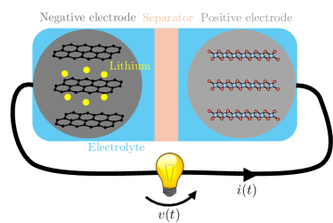
Figure 1: Illustration of a physics-based battery model with single particles and electrolyte.

A battery model (Fig. 1) allows us to simulate the terminal voltage $v(t)$ as an operator acting on the applied current $i(t)$ and depending on parameters $\theta$,

$$v(t)=F_{\theta}\{i(t)\},$$ (1)

with the variable $t$ representing time. In this work, we look at physics-based models, such as the SPM, SPMe, or DFN. These relate the terminal voltage to the applied current based on processes occurring within the battery such as diffusion and charge transfer. These depend on a set of parameters $\theta$ (Table 2 for the SPMe) and consist of systems of partial differential equations (in space and time), ordinary differential equations, differential algebraic equations (DAEs), and nonlinear operators, as set out in Appendix B for the SPMe. Note that the open circuit potentials (OCPs) of each electrode are also required. Non-invasive model parametrisation for a specific battery consists of estimating the parameters $\theta$ from current and voltage data from that battery.

1.1 Time domain voltage method

Before we look at EIS data, we briefly consider the time domain voltage method where we parametrise the model by specifying the current and minimising the difference between measured voltage and simulated voltage. An example of such data is illustrated in Fig. 2 and we might choose the optimal parameter values $\hat{\theta}$ to satisfy

$$\hat{\theta}=\arg\min_{\theta}\sum_{n=0}^{N-1}\big{(}v(t_{n})-v(t_{n},i(t),\theta,\mathrm{SOC}_{0})\big{)}^{2},$$ (2)

with $v(t_{n})$ the measured data at discrete times $t_{n}$ and $v(t_{n},i(t),\theta,\mathrm{SOC}_{0})$ the voltage simulated by the model with as initial condition $\mathrm{SOC}_{0}$ (the state-of-charge at time $t_{0}$). An alternative to the frequentist approach is the Bayesian approach, which has been used to explore the identifiability of the SPMe in [34]. Both of these types of optimisation can be performed with the open source Python package PyBOP [33], which fits PyBaMM models to data.

A drawback of only using time domain data is that the identifiability of some parameters may be poor. Hence, in this paper we will consider how to fit model parameters using impedance data, which is in the frequency domain, found from EIS measurements. In the next sections we detail how to measure EIS data and show how it can be used for model parametrisation.

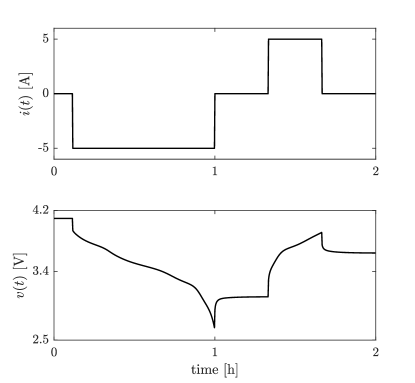
Figure 2: Illustration of a time domain simulation of the SPMe in Appendix C. The upper graph shows the applied current $i(t)$ while the lower graph shows the simulated voltage $v(t)$.

1.2 Measuring impedance data

EIS has become a widely applied technique for parametrising models [35], not only in laboratories, but also in BMS. However, one has to be careful to measure valid impedance data, that is, data satisfying the conditions of linearity and stationarity [18, 36].

A battery is in a stationary condition when it is at a fixed operating point $x_{m}$ (fixed state-of-charge and temperature), typically after a relaxation period of 2 hours or longer. The condition of linearity is satisfied when the amplitudes of the sinusoidal current or voltage perturbations around the operating point are small enough. A voltage deviation smaller than 10 mV is often considered to ensure linearity, however this depends on several factors such as the frequency, temperature, and SOC.

We choose the current as excitation,

$$i(t)=I_{k}\sin(\omega_{k}t),$$ (3)

with $I_{k}$ the amplitude, $\omega_{k}=2\pi f_{k}$ the angular frequency, and $f_{k}$ the frequency. When linearity and stationarity are satisfied during the experiment, the battery behaves as a linear time-invariant (LTI) system around the operating point $x_{m}$. Hence, after transients have faded away, the voltage response to the sinusoidal current excitation (3) yields,

$$v(t) =\text{OCV}_{m}+\mathcal{F}^{-1}\{Z_{m}(\omega)I(\omega)\}$$ (4a)

$$=\text{OCV}_{m}+\underbrace{|Z_{m}(\omega_{k})|I_{k}}_{V_{k}}\sin\big(\omega_{k}t+\underbrace{\angle Z_{m}(\omega_{k})}_{\varphi_{k}}\big{missing}),$$ (4b)

with OCV_m the open circuit voltage at operating point $x_{m}$, $\mathcal{F}^{-1}\{\cdot\}$ the inverse Fourier transform, $Z_{m}(\omega)$ the impedance at operating point $x_{m}$, and $I(\omega)$ the Fourier transform of $i(t)$. The voltage response is thus also a sinusoidal signal, superimposed on the OCV, but with a different amplitude $V_{k}$ and a phase shift $\varphi_{k}$. The impedance at angular frequency $\omega_{k}$ can then be measured from the Fourier spectra of voltage and current as

$$Z_{m}(\omega_{k})=\frac{V(\omega_{k})}{I(\omega_{k})}=\frac{V_{k}}{I_{k}}e^{j\varphi_{k}},$$ (5)

where the complex impedance can be decomposed into its real part $Z_{\mathrm{r}}(\omega_{k})$ and imaginary part $Z_{\mathrm{j}}(\omega_{k})$.

To obtain impedance data over a wide frequency range, this procedure is repeated at different angular frequencies $\omega_{k}$, which are typically logarithmically spaced from high to low. The conditions of linearity and stationarity should be checked for every frequency, which can be done by analysing the current and voltage data in the frequency domain [36], looking at the Lissajous plots [37], or, when all impedance data is collected, by using the Kramers-Kronig relations [38] or a measurement model [39, 40]. Note that for a battery, it is typically more difficult to obtain valid impedance data at low frequencies as nonlinear effects may be strong there [41].

1.3 Parametrising a model from EIS data

When measured over a wide frequency range, impedance data $Z_{m}(\omega_{k})$ reveals information about physical processes occurring at different time scales within the battery. Quantitative information about these processes can be obtained by fitting a model to the impedance data and estimating its parameters.

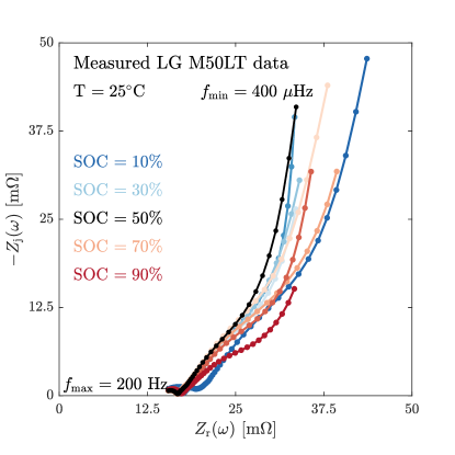
Figure 3: Nyquist plot of measured EIS data of the LG M50LT at different SOC and 25^∘C. Frequency range: [400 $\mu$Hz, 200 Hz].

To parametrise a physics-based model from measured impedance data we gather a dataset

$$\mathcal{D}=\{\omega_{k},Z_{m}(\omega_{k})\}_{k=1,...,K}^{m=1,...,M},$$ (6)

where the index $k$ runs over the different excited frequencies and $m$ runs over different operating points (e.g. different SOC). An example of such a measured dataset with $M=9$ different SOC operating points and $K=61$ frequencies, logarithmically spaced between 200 Hz and 400 $\mu$Hz, is shown in Fig. 3 for an LG M50LT battery. Some of the model parameters $\theta$ can then be estimated by minimising a chosen cost function, for instance, the sum of squares of the difference between the impedance dataset and the model’s impedance $Z_{m}(\omega,\theta)$,

$$\hat{\theta}=\arg\min_{\theta}\sum_{m=1}^{M}\sum_{k=1}^{K}|Z_{m}(\omega_{k})-Z_{m}(\omega_{k},\theta)|^{2}.$$ (7)

While it is common practice to estimate local model parameters from impedance at single operating points (for instance for an equivalent circuit model), we want to estimate global model parameters so that the set of parameters makes the model fit data at all the operating points. We do this by estimating the parameters simultaneously from impedance data at different SOC.

For relatively simple models the impedance $Z_{m}(\omega,\theta)$ can be calculated analytically by linearising the model at the operating point $x_{m}$ and transforming it into the frequency domain. However, for more complicated models, such as the SPMe or DFN, calculating an analytical expression of the impedance can become prohibitively complicated. Therefore, in this paper, we propose a fast numerical frequency domain method to obtain the model’s impedance using PyBaMM.

2 Computing numerical impedance with PyBaMM

To simulate physics-based models numerically, the spatial geometry (see Fig. 1) is typically meshed and the model is discretised on this mesh (for example, using the finite volume method [42]). It is important that sufficient discretisation points are chosen for correct simulations; we take 100 discretisation points for the radius of the particles, 100 discretisation points over the thickness of each electrode, and 20 points over the thickness of the separator. Variables evaluated over this mesh (e.g. the lithium concentration at specific points in the particles and electrolyte) are then converted into a state vector $\mathbf{x}(t)\in\mathbb{R}^{(N_{\mathbf{x}}+2)\times 1}$, with $N_{\mathbf{x}}$ is the number of states in the PyBaMM model and the additional two states being the voltage and current, and spatial operators (such as gradients and divergences) become matrices. The physics-based model of a battery then becomes a system of DAEs,

$$\mathbf{M}_{\theta}\big{(}\mathbf{x}(t)\big{)}\derivative{\mathbf{x}(t)}{t}=\mathbf{F}_{\theta}\big{(}\mathbf{x}(t)\big{)}+\mathbf{B}i(t),$$ (8)

with $\mathbf{M}_{\theta}$ the mass matrix of the system, $\mathbf{F}_{\theta}$ a vector-valued nonlinear multivariate function, and $\mathbf{B}$ a zero column vector with a unit entry in its last element. It is this system of DAEs that is solved in battery modelling software such as PyBaMM [31] to simulate the terminal voltage of a battery for a given applied current.

To obtain an impedance, the nonlinear system of DAEs (8) can be linearised around an operating point $\mathbf{x}_{m}$ and transformed into the frequency domain. The impedance at angular frequency $\omega_{k}$ can then be obtained as the scalar

$$Z_{m}(\omega_{k},\theta)=\Big{[}(j\omega_{k}\mathbf{M}_{\theta,m}-\mathbf{J}_{\theta,m})^{-1}\mathbf{B}\Big{]}_{N_{\mathbf{x}}+1},$$ (9)

where $j$ is the imaginary unit ($j^{2}=-1$), $\mathbf{J}_{\theta,m}$ is the Jacobian of $\mathbf{F}_{\theta}$ at the operating point $\mathbf{x}_{m}$,

$$\mathbf{J}_{\theta,m}=\frac{\partial\mathbf{F}_{\theta}(\mathbf{x})}{\partial\mathbf{x}}\bigg{\rvert}_{\mathbf{x}=\mathbf{x}_{m}},$$ (10)

$\mathbf{M}_{\theta,m}$ is the mass matrix evaluated at $\mathbf{x}_{m}$, and $N_{\mathbf{x}}+1$ indicates the entry for the voltage in the vector. The mathematical derivation for (9) with the definition of all of its terms is given in Appendix A.

In this work, we exploit PyBaMM to discretise the spatial dependencies of the model and compute the Jacobian $\mathbf{J}_{\theta,m}$ using automatic differentiation, which is exact. PyBaMM implements physics-based models by means of expression trees, to which parameter values $\theta$ are passed, and solves nonlinear systems of DAEs with suitable solvers.

We have developed open-source software called PyBaMM-EIS that implements this numerical frequency domain method, allowing efficient computation of the impedance of any battery model implemented in PyBaMM, at any operating point $\mathbf{x}_{m}$ during a simulation. Moreover, users can define their own model and compute an impedance from it.

3 Validation of the numerical impedance

We now validate the proposed numerical frequency domain impedance computation method by comparing it to a brute-force simulation and comparing the computation speed of the two approaches. The brute-force simulation consists of simulating the voltage response of the model for a sinusoidal current input at different frequencies and computing the impedance (5) from the Fourier spectra of these signals.

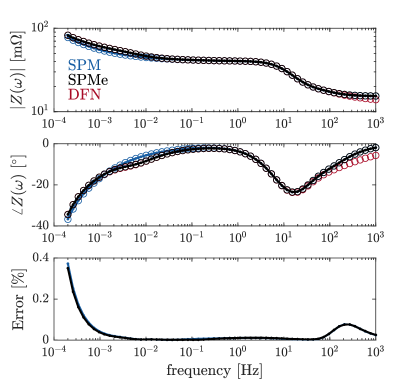
Figure 4: Bode plot of simulated impedance data for the LG M50 cell at 50% SOC for the SPM, SPMe, and DFN computed using the brute-force method ($Z_{\mathrm{bf}}(\omega)$, dots) and the numerical frequency domain method ($Z_{\mathrm{f}}(\omega)$, circles), and their relative error defined as $\text{Error [\%]}=100\frac{|Z_{\mathrm{bf}}(\omega)-Z_{\mathrm{f}}(\omega)|}{|Z_{\mathrm{f}}(\omega)|}$. The time domain DFN impedance is not shown due to a prohibitively long computation time.

Model	$N_{\mathbf{x}}$	Computation time
		Brute-force	Freq. domain
SPM	204	11.8 s	21.3 ms
SPMe	424	32.8 s	415 ms
DFN	20422	–	925 ms

Table 1: Number of states $N_{\mathbf{x}}$ and representative computation times for the impedance of different models and solution methods (averaged over 10 runs). The time domain DFN computation time was prohibitively long.

We consider the SPM, SPMe, and DFN models with double-layer capacitance implemented in PyBaMM with the parameter set of chen2020 [43] for the LG M50 cell. Fig. 4 shows a Bode plot of the EIS spectra of these models calculated using the brute-force and frequency domain approaches. Within PyBaMM the models were discretised in space using the finite volume method resulting in a DAE system with the number of states $N_{\mathbf{x}}$ listed in Table 1. Note that the DFN has the most states and the SPM the least. The impedance response was computed for an operating point at 50% SOC and 25^∘C, with 60 logarithmically spaced frequencies between 200 $\mu$Hz and 1 kHz. For the brute-force sinusoidal excitation, we chose an amplitude of $I_{k}=100$ mA and simulated the response for 10 periods. Only the 5 last periods were retained to discard transient effects. To obtain accurate simulations over this wide frequency range, we set the absolute tolerance of the solver to $10^{-9}$. The impedance was then computed from the ratio of voltage and current Fourier spectra (5). We used PyBaMM-EIS, with the same PyBaMM specifications, to compute the frequency domain numerical impedance.

We observe that both methods give excellent agreement with one another, with a relative error smaller than $0.4$% for all models over the entire frequency range. Note that the frequency domain approach computes the exact linearisation, while the brute-force approach is only exact when the amplitude of the sinusoidal excitation is small enough such that linearity is satisfied [36]. Battery models are typically more nonlinear at low frequencies due to the nonlinear OCV, which explains the significantly larger error at low frequencies. The computation times for obtaining the data in Fig. 4 are listed in Table 1 (note that the brute-force DFN simulation did not finish in a reasonable time due to the large number of states). We conclude that the numerical frequency domain approach is faster and provides us with accurate impedance data.

4 Comparing the impedance of different models

Using PyBaMM-EIS, we now compare the impedance response of different models for the chen2020 parameter set for the LG M50 cell. We found we needed 100 discretisation points in the particle to adequately resolve the impedance behaviour, especially in the high frequency diffusion region, and doing so made our results slightly differ from those of [30].

Fig. 5 shows a Nyquist plot of the impedance for the SPM, SPMe, and DFN, as implemented in PyBaMM, at 50% SOC and 25^∘ C (note that this is the same data as shown in Fig. 4). For each of these models, we notice two main features: a semi-circle (linked with charge transfer kinetics) and a low frequency diffusion tail. An analytical form of the SPM solid-state diffusion tail can be found in [29], which starts with a 45^∘ slope and goes towards a capacitive behaviour (vertical line in the Nyquist plot). We see the same here. The models where electrolyte dynamics are considered (SPMe and DFN) have a diffusion tail with an additional “bump”, linked with electrolyte diffusion. This “bump” is often present in measured impedance (see Fig. 3), indeed, measured impedance data rarely shows a diffusion tail with a 45^∘ slope that can be modelled with a Warburg element [44, 45, 46]. This suggests that it is worthwhile to work with models that consider electrolyte dynamics (at the cost of a more complicated model). Also note that the SPMe and DFN differ only at high frequencies (which matter less for simulations of real battery behaviour), as can be observed in the Bode plot of Fig. 4.

As the SPM lacks electrolyte dynamics—which are notable in impedance measurements—and the DFN has significantly more parameters and needs longer solve times than the SPMe while showing similar impedance data, we will work with the SPMe for the remainder of this paper.

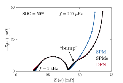
Figure 5: Nyquist plot of the EIS spectra of the SPM, SPMe, and DFN model at 50% SOC of the LG M50 cell (Chen2020 dataset) computed using the frequency domain method. Frequency range: [200 $\mu$Hz, 1 kHz]. The DFN overlaps with the SPMe, except at high frequencies. Note that we have changed the contact resistance of the SPM to match with the other models.

5 Impedance analysis of the SPMe

We consider the SPMe with double-layer capacitance defined in Appendix B, which is an extension of [10, 11]. This model depends on the OCPs of both electrodes and has 31 parameters, which are listed in Table 2. Note that two of these parameters are physical constants (the Faraday constant and ideal gas constant), and hence known, and one of the parameters is the temperature which can be measured, so in total, there remain 28 unknown parameters to simulate this model. Typically, the number of necessary parameters to simulate the model can be reduced by grouping them, which is discussed next. We then study the physical processes in the model (occurring at different time scales) to show how the impedance depends on SOC and changes when varying the grouped parameters.

5.1 Grouping model parameters

Not all of the model parameters can be estimated independently from current and voltage data, as some group together in the model. By grouping parameters, physics-based models can be rewritten with fewer parameters [47]. Grouped parameters naturally arise when non-dimensionalising the model variables. This has been done for the SPM by Bizeray et al. [29], for the SPM with double-layer capacitance by Kirk et al. [23], and for the SPMe without double-layer capacitance by Marquis et al. [10]. Grouping the parameters of the DFN model has been studied in [48] and in [15] for lithium metal batteries.

	Model parameters
$F$	Faraday constant [C/mol]
$R_{\mathrm{g}}$	Ideal gas constant [J/(mol.K)]
T	Ambient temperature [K]
$\alpha_{\pm}$	Electrode active material volume fraction
$\varepsilon_{\pm}$	Electrode porosity
$\varepsilon_{\mathrm{sep}}$	Separator porosity
$c_{\pm,\mathrm{max}}$	Electrode active material max. conc. [mol/m3]
$L_{\pm}$	Electrode thickness [m]
$L$	Total cell (electrodes & separator) thickness [m]
$A$	Electrode area [m2]
$R_{\pm}$	Particle radius [m]
$D_{\pm}$	Diffusivity in the particles [m2/s]
$D_{\mathrm{e}}$	Reference electrolyte diffusivity [m2/s]
$C_{\mathrm{dl},\pm}$	Electrode double-layer capacity [F/m2]
$m_{\pm}$	Ref. exch. current dens. [(A/m2)(m3/mol)1.5]
$t^{+}$	Cation transference number
$b$	Bruggeman coefficient
$c_{\pm}^{*0\%}$	Particle concentration at 0% SOC [mol/m3]
$c_{\pm}^{*100\%}$	Particle concentration at 100% SOC [mol/m3]
$c_{\mathrm{e},0}$	Initial electrolyte concentration [mol/m3]
$R_{0}$	Series resistance [$\Omega$]

Grouped parameters $\theta$
$Q^{\mathrm{th}}_{\pm}=F\alpha_{\pm}c_{\pm,\mathrm{max}}L_{\pm}A$	Theor. electrode capacity [As]
$\displaystyle Q^{\mathrm{e}}=F\varepsilon_{\text{sep}}c_{\mathrm{e},0}LA$	Ref. electrolyte capacity [As]
$\displaystyle\tau^{\mathrm{d}}_{\pm}=\frac{R^{2}_{\pm}}{D_{\pm}}$	Particle diff. time scale [s]
$\displaystyle\tau^{\mathrm{e}}_{\pm}=\frac{\varepsilon_{\text{sep}}L^{2}}{\varepsilon_{\pm}^{b_{\pm}}D_{\mathrm{e}}}$	Electrolyte diff. time scale [s]
$\displaystyle\tau^{\mathrm{e}}_{\mathrm{sep}}=\frac{L^{2}}{\varepsilon_{\mathrm{sep}}^{b_{\mathrm{sep}}-1}D_{\mathrm{e}}}$	Electrol. diff. time scale sep. [s]
$\displaystyle\tau^{\mathrm{ct}}_{\pm}=\frac{FR_{\pm}}{m_{\pm}\sqrt{c_{\mathrm{e},0}}}$	Charge transfer time scale [s]
$\displaystyle C_{\pm}=\frac{3\alpha_{\pm}C_{\mathrm{dl},\pm}L_{\pm}A}{R_{\pm}}$	Double-layer capacitance [F]
$\zeta_{\pm}=\varepsilon_{\pm}/\varepsilon_{\mathrm{sep}}$	Relative electrode porosity
$\ell_{\pm}=L_{\pm}/L$	Relative electrode thicknesses
$\displaystyle c_{\pm}^{0\%}=c_{\pm}^{*0\%}/c_{\pm,\mathrm{max}}$	Stoichiometry at 0% SOC
$\displaystyle c_{\pm}^{100\%}=c_{\pm}^{*100\%}/c_{\pm,\mathrm{max}}$	Stoichiometry at 100% SOC
$t^{+}$	Cation transference number
$R_{\mathrm{0}}$	Series resistance [$\Omega$]

Table 2: Model parameters of the SPMe with double-layer capacitance detailed in Appendix B and grouped parameters (see Appendix C).

In Appendix C, we have grouped the parameters of our SPMe with double-layer capacitance (keeping only the dimensions of time, current, and voltage) and obtained 22 grouped parameters, which we list in Table 2. Note that all these grouped parameters have units that depend upon seconds, Amperes, and Volts.

The theoretical electrode capacities $Q^{\mathrm{th}}_{\pm}$ are related to the stoichiometries at 0% and 100% SOC through [23],

$$Q^{\mathrm{th}}_{\pm}=\mp\frac{Q_{\mathrm{meas}}}{c_{\pm}^{100\%}-c_{\pm}^{0\%}},$$ (11)

with $Q_{\mathrm{meas}}$ the measured electrode capacity, which can be measured (e.g. $Q_{\mathrm{meas}}=5.15\ \text{Ah}=18551\ \text{As}$ in the chen2020 parameter set for the LG M50). This reduces the number of grouped parameters to be estimated by two when $Q_{\mathrm{meas}}$ is known.

The time scales $\tau^{\mathrm{ct}}_{\pm}$ are used to represent the charge transfer kinetics (as these arise when non-dimensionalising the model equations). However, representing charge transfer kinetics with a resistance makes physically more sense. Typical charge transfer resistances, which have values the order of magnitude of the diameter of the semi-circles in the impedance data, could be used instead [23]

$$R^{\mathrm{typ}}_{\mathrm{ct},\pm} =\frac{2R_{\mathrm{g}}\mathrm{T}R_{\pm}}{3FAL_{\pm}\alpha_{\pm}m_{\pm}c_{\pm,\mathrm{max}}\sqrt{c_{\mathrm{e},0}}}=\frac{2R_{\mathrm{g}}T}{F}\frac{\tau^{\mathrm{ct}}_{\pm}}{3Q^{\mathrm{th}}_{\pm}}.$$ (12)

The SPMe of Appendix C can be simulated knowing just the grouped parameters of Table 2 and the open circuit potentials (OCP) of each electrode, showing identical behaviour as the SPMe implemented in PyBaMM.

5.2 Model time scales

The power of EIS data is that it allows us to distinguish between different physical processes that occur at different time scales within the battery. We illustrate this for the grouped SPMe in Fig. 6. The different processes that we can distinguish at different time scales $\tau$ are the following:

• $\tau<1$ ms ($f>1$ kHz): At very short time scales the SPMe acts as a resistance, that is, the series resistance $R_{0}$.

• 1 ms $<\tau<$ 1 s (1 Hz $<f<$ 1 kHz): For these time scales, the dominant process of the SPMe is charge transfer, represented by two semi-circles in the Nyquist plot (one for each electrode). The time scale of this process is related to the charge transfer time scales $\tau^{\mathrm{ct}}_{\pm}$. However, as discussed above, their values do not represent the actual time scale. A better value would be $\tilde{\tau}^{\mathrm{ct}}_{\pm}=R^{\mathrm{typ}}_{\mathrm{ct},\pm}C_{\pm}$ (which is the time scale related to the resonating frequency of the $RC$-pair). Numerical values for the chen2020 parameter set yield $\tilde{\tau}^{\mathrm{ct}}_{+}=1.5$ ms and $\tilde{\tau}^{\mathrm{ct}}_{-}=15$ ms.

• 1 s $<\tau<$ 1000 s (1 mHz $<f<$ 1 Hz): In this range we have the processes of diffusion within the electrolyte, whose time scales are $\tau^{\mathrm{e}}_{\pm}$ and $\tau^{\mathrm{e}}_{\mathrm{sep}}$. The effect on the impedance is the “bump” in the diffusion tail. Numerical values for the chen2020 parameter set yield $\tau^{\mathrm{e}}_{+}=409.2$ s, $\tau^{\mathrm{e}}_{-}=634.7$ s, and $\tau^{\mathrm{e}}_{\mathrm{sep}}=246.2$ s.

• $\tau>$ 1 s ($f<$ 1 Hz): The longest time scales are related to diffusion within the particles, related to $\tau_{\pm}^{\mathrm{d}}$. The effect on the impedance is the diffusion tail. Numerical values for the chen2020 parameter set yield $\tau_{+}^{\mathrm{d}}=6812$ s and $\tau_{-}^{\mathrm{d}}=1041$ s.

The frequency ranges chosen here are not hard bounds and these values vary from battery to battery. Also note that frequency ranges of different physical processes may overlap. The electrolyte diffusion and particle diffusion time scales overlap in this example, and so do the charge transfer time scales in positive and negative electrodes. Due to the overlap in time scales we get the black line in Fig. 6 as the impedance, instead of the (ideal) dotted line.

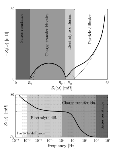
Figure 6: Impedance of the SPMe related to different physical processes occurring at different time scales. The dotted line in the Nyquist plot shows the impedance if the time scales of each process were perfectly separated. In reality they are not and we get the black line.

5.3 Impedance at different operating points

In stationary conditions, the SOC sets the particle stoichiometry $c_{\pm}$ (which is constant over the particle radius) by linear interpolation

$$c_{\pm}=c_{\pm}^{0\%}+\frac{\text{SOC}}{100}\left(c_{\pm}^{100\%}-c_{\pm}^{0\%}\right),$$ (13)

with $c_{\pm}^{0\%}$ and $c_{\pm}^{100\%}$, respectively, the stoichiometries at 0% and 100% SOC. Linearising the model at different SOC operating points $x_{m}$ (corresponding to different stoichiometries $c_{m,\pm}$) results in different impedance data, as can be seen in Fig. 7 for the grouped SPMe.

We note that the diameter of the semi-circles changes with SOC. This diameter is typically called the charge transfer resistance and is the derivative of the voltage contribution from the spatially averaged overpotential $\mkern 1.5mu\overline{\mkern-1.5mu\eta_{\pm}\mkern-1.5mu}\mkern 1.5mu$, with respect to the current, evaluated at the operating point $x_{m}$ (containing $i=0$). From Appendix D,

$$R_{\mathrm{ct},m,\pm} \approx\frac{R_{\mathrm{ct},\pm}^{\mathrm{typ}}}{2\sqrt{c_{m,\pm}(1-c_{m,\pm})}}\frac{1}{\mkern 1.5mu\overline{\mkern-1.5mu\sqrt{c_{\mathrm{e},\pm}}\mkern-1.5mu}\mkern 1.5mu\big{\rvert}_{x_{m}}}.$$ (14)

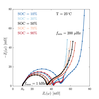
Figure 7: EIS spectra of the grouped SPMe (see Appendix C) at different SOC operating points and at 25^∘C. Frequency range: [200 $\mu$Hz, 1 kHz]. The model parameter values are listed as $\theta$ in Table 3. Note that the impedance at 10 % SOC has been cut-off.

High and low stoichiometries $c_{m,\pm}$ (related to high and low SOC) give higher charge-transfer resistance values, while the middle SOC range gives lower charge transfer resistance values. This is exactly what we see from the data.

The diffusion tail too changes strongly with SOC. This can be explained from (C.7). The diffusion tail impedance is related to the derivative

$$\frac{\mathrm{d}U_{\pm}(c_{\pm}|_{r=1})}{\mathrm{d}i}\bigg{\rvert}_{x_{m}}=\underbrace{U_{\pm}^{\prime}(c_{m,\pm})}_{\text{slope of OCP}}\frac{\mathrm{d}c_{\pm}|_{r=1}}{\mathrm{d}i}\bigg{\rvert}_{x_{m}},$$ (15)

and is proportional to the slope of the OCP [23, 29]. This slope strongly depends on the stoichiometries $c_{m,\pm}$, and, hence, on the SOC (see Fig. 9). The OCP slopes here are largest at 10% SOC, giving the largest diffusion tail. At an SOC where an OCP is flat (a zero slope), there will be no contribution of this electrode in the diffusion tail.

The series resistance $R_{0}$ in this model does not depend on SOC, and hence, the leftmost intercept with the real axis stays the same for all SOC.

5.4 Impedance sensitivity to the grouped parameters

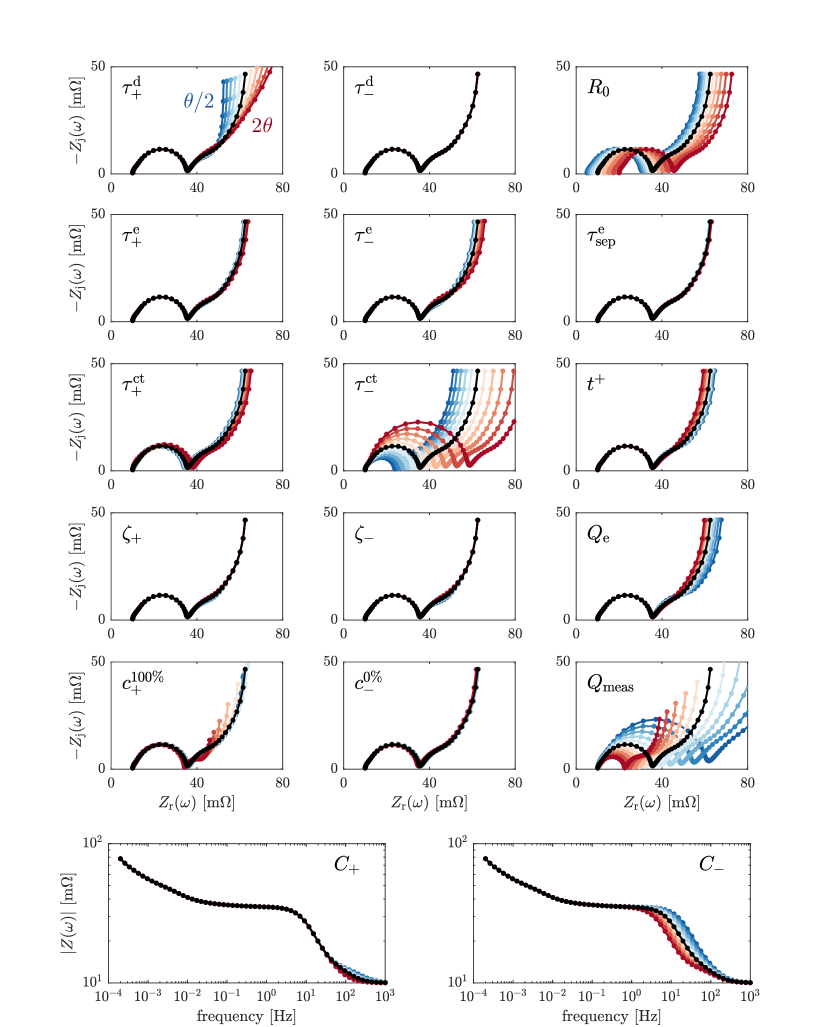
Figure 8: Impedance of the SPMe at 50% SOC and 25 ${}^{\circ}\mathrm{C}$ when varying the grouped parameters one by one. Parameters are perturbed with logarithmic spacing in the range $[0.5\theta,2\theta]$ (blue to red) with $\theta$ the Chen2020 parameters and $R_{0}=10$ m$\Omega$ (black). Frequency range: [200 $\mu$Hz, 1 kHz]. Note that most impedance are shown on a Nyquist plot, while the bottom two figures for the capacitances are Bode magnitude plots.

Fig. 8 shows the impedance of the SPMe for variations of the grouped parameters $\theta$ of Table 2. We describe the effect of each of these parameters:

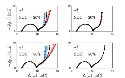
Figure 11: Sensitivity of the SPMe impedance to the particle diffusion time scales $\tau_{\pm}^{\mathrm{d}}$. The impedance is insensitive to $\tau_{\pm}^{\mathrm{d}}$ at SOC where the OCP $U_{\pm}$ is flat. The OCP of graphite has several plateaus (see Fig. 9), which explains why $\tau_{-}^{\mathrm{d}}$ is not identifiable at certain SOC. Parameters are perturbed in the range $[0.5\theta,2\theta]$ (blue to red) with $\theta$ the Chen2020 parameters with contact resistance of 10 m$\Omega$ (black). Frequency range: [200 $\mu$Hz, 1 kHz].

• The diffusion time scales in the particles have an effect at low frequencies in the diffusion tail: these are associated with the frequency where the diffusion tail changes from the 45-ish degree slope to the capacitative behaviour. Because these parameters have an effect at (very) low frequencies, long impedance experiments are needed to estimate them. At 50% SOC, as shown in the figure, $\tau^{\mathrm{d}}_{-}$ seems not to affect the impedance. This is because the slope of the negative OCP is nearly flat at that particular SOC [29]. At different SOC, the diffusion timescale of different electrodes may be better identifiable, as can be seen in Appendix, Fig. 11. This gives us an incentive to estimate the model parameters from impedance at different SOC, as in (7).

• The series resistance simply shifts the impedance along the horizontal direction.

• The electrolyte diffusion timescales have an effect on the time scale of the “bump”, and hence, at which frequencies it interacts with the particle diffusion. Note that the electrolyte diffusion time scale in the separator $\tau^{\mathrm{e}}_{\mathrm{sep}}$ has nearly no effect on the impedance.

• The charge transfer time scales change the diameter of the semi-circles. The change for the negative electrode is observed to be significantly larger than for the positive one. The diameter of the semi-circles is larger around 0 and 100% SOC, as can be seen in Fig. 7, making it easier to estimate these parameters. This again gives an incentive to estimate the model parameters from impedance at different SOC levels.

• The cation transference number slightly changes the initial slope and resistance of the diffusion tail.

• The relative electrode porosities have a small effect in the middle part of the diffusion tail.

• The reference electrolyte capacity changes the initial slope and resistance of the diffusion tail.

• The stoichiometries at 0 and 100% SOC change the stoichiometry at the particular SOC (13), and, hence, the width of the semi-circle (14) and the diffusion tail (15).

• The measured capacity changes the total size of the impedance. Batteries with a large capacity have a small impedance, and vice versa. Also recall that the theoretical electrode capacities $Q_{\pm}^{\mathrm{th}}$ can be calculated from $Q_{\mathrm{meas}}$, $c_{\pm}^{0\%}$, and $c_{\pm}^{100\%}$ (11).

• The effect of the double-layer capacitances cannot easily be seen on Nyquist charts, as it only changes the frequency dependence of the points on the semi-circle, but can be seen on a magnitude Bode plot. Here we note that the charge-transfer kinetics at the surface of the positive particles are faster than the negative ones.

As all these grouped parameters have a unique effect on the impedance, they can possibly be estimated from impedance data (depending on the frequency range and how strongly the processes are present in the impedance).

6 Parametrisation of the SPMe in simulations

We now study the estimation of the grouped SPMe parameters from impedance data by fitting the SPMe to simulated impedance data (where the true parameters are known).

The grouped parameters $c_{\pm}^{0\%}$ and $c_{\pm}^{100\%}$ are typically estimated from OCP and OCV data [23]. However, instead of fixing these values from OCP and OCV data, we will estimate them from impedance data at different SOC, and then set $Q^{\mathrm{th}}_{\pm}$ from (11).

Assuming that the relative thicknesses $\ell_{\pm}$ are known, the remaining grouped model parameters to estimate from measured impedance data are

$$\theta=[ \tau^{\mathrm{d}}_{+},\tau^{\mathrm{e}}_{+},\tau^{\mathrm{ct}}_{+},C_{+},\zeta_{+},c_{+}^{0\%},c_{+}^{100\%},$$

$$\tau^{\mathrm{d}}_{-},\tau^{\mathrm{e}}_{-},\tau^{\mathrm{ct}}_{-},C_{-},\zeta_{-},c_{-}^{0\%},c_{-}^{100\%},$$

$$\tau^{\mathrm{e}}_{\mathrm{sep}},Q^{\mathrm{e}},t^{+},R_{0}]\qquad\in\mathbb{R}_{+}^{18\times 1}.$$ (16)

The values of the true grouped parameters $\theta$ for the simulations are calculated from the Chen2020 parameter set and listed in Table 3.

6.1 Estimation from impedance data

We first study the parameter estimation from the simulated SPMe impedance data of Fig. 7. The impedance dataset (6) has $K=60$ frequencies, logarithmically spaced between 200 $\mu$Hz and 1 kHz, and $M=9$ different SOC levels (10%, 20%,…, 90%). We estimate the grouped parameters $\theta$ (16) by minimising the least squares cost function (7). The optimisation is performed with the multi-fitting problem class in PyBOP, using particle swarm optimisation (PSO) as the optimiser, with the boundaries for the 18-dimensional search space given in Table 3. We allow for a maximum of 1000 iterations and run the optimisation 10 times. Although the fitting is done over all SOC, it is instructive to examine the mean relative fitting errors (FE) at the different SOC levels

$$\mathrm{FE}_{m}\ [\%]=\frac{100}{K}\sum_{k=1}^{K}\frac{|Z_{m}(\omega_{k})-Z_{m}(\omega_{k},\hat{\theta})|}{|Z_{m}(\omega_{k})|}.$$ (17)

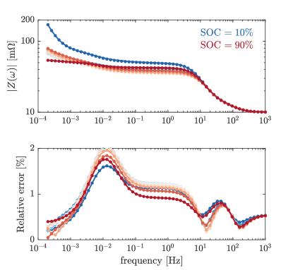
Figure 12: Fits of simulated SPMe impedance data and relative error. The estimated parameters are listed in Table 3 .

These are listed in Table 3 for the best fit of the 10 runs and the data over frequency is shown in Appendix, Fig. 12. The fitting errors are under 1% for all SOC levels.

The estimated parameters $\hat{\theta}$ of the best fit of the 10 runs are listed in Table 3. As an indication of the identifiability of the grouped parameters, we also list the relative standard deviation $\sigma_{\hat{\theta}}/\hat{\theta}$ over the 10 runs; we would expect accurately identifiable parameter from the data to have a small standard deviation. However, the cost function is highly non-convex, and, hence, this metric for the identifiability may depend on the optimiser and initial point. A better way would be to look at the Fisher information matrix [49]. The parameters related to large features can be identified accurately from impedance data (e.g. the stoichiometry bounds, series resistance, particle diffusion time scales, and charge transfer time scale of the large semi-circle). The estimated parameters related to the electrolyte diffusion and separator are less accurate, but these parameters related to small features in the impedance have little effect on the behaviour of the battery. The grouped model parameters are also all attributed to the correct electrode.

			Impedance data		Voltage data
Parameter	Optimisation bounds	$\theta$	$\hat{\theta}$	$\sigma_{\hat{\theta}}/\hat{\theta}$ [%]	$\hat{\theta}$	$\sigma_{\hat{\theta}}/\hat{\theta}$ [%]
$Q_{\mathrm{meas}}$ [As]		18551
$l_{+}$		0.4375
$l_{-}$		0.4930
$\tau^{\mathrm{d}}_{+}$ [s]	[5e2,1e4]	6812	6682	0.38	6831	0.53
$\tau^{\mathrm{d}}_{-}$ [s]	[5e2,1e4]	1041	1020	0.93	1065	1.48
$\tau^{\mathrm{e}}_{+}$ [s]	[2e2,1e3]	409.2	200.0	0.011	948.0	1.24
$\tau^{\mathrm{e}}_{-}$ [s]	[2e2,1e3]	634.7	403.5	20.9	209.9	53.7
$\tau^{\mathrm{e}}_{\mathrm{sep}}$ [s]	[2e2,1e3]	246.2	200.0	0.61	200.7	0.59
$\zeta_{+}$	[0.5,1.5]	0.7128	0.500	0.0019	0.7573	3.13
$\zeta_{-}$	[0.5,1.5]	0.5319	1.500	41.9	0.5420	3.09
$Q_{\mathrm{e}}$ [As]	[5e2,1e3]	804.8	500.0	8.20	797.9	2.12
$\tau^{\mathrm{ct}}_{+}$ [s]	[1e3,5e4]	4657	5158	26.5	6244	6.92
$\tau^{\mathrm{ct}}_{-}$ [s]	[1e3,5e4]	27592	27746	5.07	13255	8.38
$C_{+}$ [F]	[0,1]	0.5935	0.6178	13.9	1.2e-4	167
$C_{-}$ [F]	[0,1]	0.6719	0.6953	8.68	0.9966	4.04
$c^{0\%}_{+}$	[0.8,0.9]	0.8540	0.8548	0.10	–	–
$c^{0\%}_{-}$	[0,0.1]	0.02635	0.02634	11.8	–	–
$c^{100\%}_{+}$	[0.2,0.3]	0.2638	0.2642	0.22	–	–
$c^{100\%}_{-}$	[0.85,0.95]	0.9106	0.9092	0.31	–	–
$t^{+}$	[0.2,0.5]	0.2594	0.2647	9.16	0.2025	28.7
$R_{0}$ [$\Omega$]	[0,0.05]	0.01	0.0101	1.22	0.0148	8.56

$m$	1	2	3	4	5	6	7	8	9
SOCm [%]	10	20	30	40	50	60	70	80	90
FEm [%]	0.87	0.97	0.96	0.97	0.94	0.94	0.90	0.86	0.84

Table 3: Parametrisation of the grouped SPMe from simulated impedance data and time domain voltage data with particle swarm optimisation in PyBOP. We list the optimisation bounds, true parameters $\theta$, estimated parameters $\hat{\theta}$ (lowest cost of 10 runs), and relative standard deviation $\sigma_{\hat{\theta}}/\hat{\theta}$ (over 10 runs). The impedance data is shown in Fig. 7 and the time domain voltage data in Fig. 2. The average computation times (run parallel on 16 AMD 7950X cores) for the parametrisation from impedance and voltage data are 441 s and 613 s, respectively. Better estimates for the electrolyte diffusion parameters can be obtained using other optimisers at the cost of longer computation times. The fitting errors (17) of the impedance at different SOC are also listed.

6.2 Comparison with time domain data

Now we study the parameter estimation from the simulated SPMe time domain voltage data of Fig. 2. The dataset consists of 7 minutes resting at 90% SOC (starting from steady-state), then a -5 A discharge for 53 minutes, 20 minutes rest, 5 A charge for 20 min, and 20 minutes rest again (resulting in a total experiment time of 2 h). The data is simulated with a time step of $10$ s, resulting in $N=720$ data points. Note that measuring this dataset would take less time than measuring the impedance dataset from Fig. 7. We estimate the grouped parameters $\theta$ (16) by minimising the least squares cost function (2). The optimisation is performed in PyBOP, using PSO as the optimiser, with the same boundaries for the 18-dimensional search space given in Table 3. We allow for a maximum of 1000 iterations and run the optimisation 10 times. The stoichiometries $c_{\pm}^{0\%}$ and $c_{\pm}^{100\%}$ were not estimated as this led to convergence issues of the optimiser, they are assumed known for this simulation.

Accurate fits of the time domain voltage data were obtained, with the estimated parameters of the best fit and the relative standard deviations over the 10 runs listed in Table 3. For this specific simulation, we conclude that the long time scale parameters are identified with similar precision from the voltage time domain data and impedance data, while the short time scale parameters are better identified from impedance data (the sampling period of 10 s in the voltage time domain data does not allow to see the fast processes occurring in the battery).

The comparison of the different sources of data discussed above suggests an extension of the work presented here, which we will explore elsewhere. We could exploit the strengths of both the time domain voltage and the frequency domain EIS data by estimating model parameters using a weighted cost function

$$\hat{\theta}=\arg\min_{\theta}w_{1}C_{\mathrm{voltage}}(\theta)+w_{2}C_{\mathrm{EIS}}(\theta),$$ (18)

where $w_{1}$ and $w_{2}$ are weights, and $C_{\mathrm{voltage}}$ and $C_{\mathrm{EIS}}$ are, respectively, the time domain voltage data (2) and EIS data (7) cost functions.

7 Parametrisation of LG M50LT batteries from measured data

We now undertake to parametrise the grouped SPMe from measured data of a LG M50LT cell. This cell has a graphite anode and NMC cathode, and operates between 2.5 V and 4.2 V. The measured cell capacity is $Q_{\mathrm{meas}}=4.885$ Ah. Open circuit potentials have been obtained by tearing down the cell (provided by About:Energy (personal communication)) and are shown in Fig. 9 for the provided stoichiometric bounds.

$m$	1	2	3	4	5	6	7	8	9
SOCm [%]	10	20	30	40	50	60	70	80	90
OCVm [V]	3.3909	3.4998	3.5893	3.648	3.728	3.856	3.931	4.038	4.084
$\mathrm{FE}_{m}$ [%]	–	3.51	3.24	2.47	5.79	3.26	2.35	1.78	–

Table 4: Measurement information about the considered operating points of the LG M50LT. The ambient temperature for all the operating points is 25^∘C.

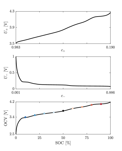
Figure 9: OCV and OCP data of the LG M50LT battery. The dots indicate the SOCs and OCVs at which the impedance of Fig. 3 is measured.

We performed EIS measurements at different operating points detailed in Table 4 and shown as dots in Fig. 9 with a Gamry Interface 5000P. The battery was first charged to 4.2 V and this voltage was held constant until the current was smaller than 50 mA. The battery was then discharged at C/10 in steps of 10% SOC (with $Q_{\mathrm{meas}}/10=0.4885$ A for periods of 1 h), followed by 4 h of zero current relaxation to reach steady-state for the EIS measurement. EIS was measured in the frequency range [400 $\mu$Hz, 200 Hz] with 10 logarithmically distributed frequencies per decade. Hybrid EIS was used (a current is applied, but a voltage perturbation is chosen by the user) with a DC current of 0 A and a sinusoidal voltage perturbation of 10 mV amplitude. A Nyquist plot of the measured impedance data is shown in Fig. 3 . The conditions of linearity and stationarity were checked from the Lissajous curves and using the measurement model toolbox of [40].

The grouped SPMe parameters $\theta$ (16) are estimated for the impedance data between 20% and 80% SOC (the 10% and 100% SOC data were hard to fit). The cost function (7), with $M=7$ and $K=61$, was minimised with 100 iterations of SciPy differential evolution. The estimated grouped parameters are listed in Table 5, with the fits shown in Fig. 10, and the average fitting errors listed in Table 4. Fits at (very) low frequencies are relatively poor, but for higher frequencies we obtained better results. At low frequencies, the impedance is strongly dependent on the slope of the OCPs, and hence on the OCP data and balancing, making it hard to obtain good fits. Moreover, due to hysteresis, the OCPs may be dependent on the direction with which we have approached the operating point (charging or discharging) and the SPMe may not be sufficiently detailed to model measured impedance data well.

We have not explored fitting the measured data with other models but there are many possible extensions that might improve the fit of the impedance response to measured data. These include considering the diffusivities in the particles to change with SOC (for example non-ideal diffusivity based on OCP (chemical) gradients as in [50] and used in [51]) or considering a distribution of particle size using multi-particle models [12], as well as the many other models available in PyBaMM.

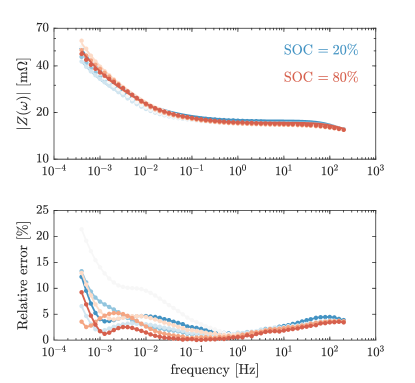
Figure 10: SPMe fits to measurements LG M50LT battery.

$\tau^{\mathrm{d}}_{+}=9065$ s	$\tau^{\mathrm{d}}_{-}=1096$ s	$R_{0}=14.63$ m$\Omega$
$\tau^{\mathrm{e}}_{+}=220.6$ s	$\tau^{\mathrm{e}}_{-}=511.2$ s	$\tau^{\mathrm{e}}_{\mathrm{sep}}=216.2$ s
$\zeta_{+}=0.792$	$\zeta_{-}=0.964$	$Q_{\mathrm{e}}=819.4$ As
$\tau^{\mathrm{ct}}_{+}=1737$ s	$\tau^{\mathrm{ct}}_{-}=1236$ s	$t^{+}=0.493$
$C_{+}=0.733$ F	$C_{-}=0.726$ F	$l_{+}=0.3697$
$c^{0\%}_{+}=0.985$	$c^{0\%}_{-}=0.00176$	$l_{-}=0.551$
$c^{100\%}_{+}=0.173$	$c^{100\%}_{-}=0.864$	$Q_{\mathrm{meas}}=17586$ As

Table 5: Estimated grouped parameters LG M50LT.

8 Conclusions

In this work, we have proposed a numerical approach to compute the impedance of physics-based models, which we have implemented under PyBaMM-EIS. The method consists of discretising the model dynamics in space, locally linearising the resulting nonlinear system of DAEs using automatic differentiation, transforming the linearised equations in the frequency domain, and solving them for the impedance. This tool allows us to evaluate impedance data of any model implemented in PyBaMM at any operating point. Moreover, it is significantly faster than doing “brute-force” simulations while giving comparable results.

We have analysed the impedance of different physics-based models (SPM, SPMe, and DFN), and have shown that it is essential to consider electrolyte dynamics (which add a “bump” in the diffusion tail that is also present in measured data). The DFN has similar impedance to the SPMe, but it is more expensive to simulate and has more parameters. Therefore, we conclude that much of the behaviour of the battery can be explained by analysing the impedance of the SPMe.

We have provided the model equations for the SPMe with double-layer capacitance, and grouped the parameters of this model to determine a minimal set of parameters required for simulations. Our grouped parameter SPMe gives identical results to PyBaMM’s SPMe. We identified how different features in the impedance of this model depend on SOC, and a sensitivity analysis of the impedance revealed the grouped parameters that have a significant effect on the impedance.

We estimated 18 grouped parameters of the SPMe using simulated voltage data and impedance data. Crucially, we fit impedance data across different SOC simultaneously in order to increase the identifiability of the parameters. We found that simulated EIS data could be fitted accurately, with most grouped parameters well estimated. The exceptions were those parameters related to small features in the impedance (which have little effect on the behaviour of the battery), for example the parameters of the separator. Hence, EIS can be used effectively to parametrise the SPMe. Comparing the informativity of simulated impedance and time domain voltage data, we found that the long time scale parameters (e.g. particle diffusion time scales) can be estimated accurately from both, but the short time scale parameters are better estimated from impedance data. We therefore suggest exploring both sources of data for parameter estimation.

To demonstrate how the methodology can be used in practice, we performed the parametrisation of the SPMe for a commercial LG M50LT battery from measured impedance and OCP data. The fit was good in the higher frequency region, but less good at lower frequencies. We have discussed the causes of this and suggested some possible extensions to the model for improving the fitting of measured impedance data. As PyBaMM-EIS can compute impedance data for any model implemented in PyBaMM, additional physical mechanisms can be added to the model and used for improving the quality of the fits.

We believe that the methodology presented in this paper gives a practical method for fitting a large class of models to EIS data. The use of automatic differentiation combined with working in the frequency domain dramatically reduces the computation time, and fitting the parameters across many SOC levels gives accurate estimations for most parameters. Moreover, the procedure presented can be complemented by using both time domain voltage and EIS as sources of data.

Appendix A: Numerical impedance computation

Software, such as PyBaMM, simulate a battery by integrating a system of DAEs

$$\overline{\mathbf{M}}_{\theta}\big{(}\overline{\mathbf{x}}(t)\big{)}\derivative{\overline{\mathbf{x}}(t)}{t}=\overline{\mathbf{F}}_{\theta}\big{(}\overline{\mathbf{x}}(t),t\big{)},$$ (A.1)

where $\overline{\mathbf{M}}_{\theta}\in\mathbb{R}^{N_{\mathbf{x}}\times N_{\mathbf{x}}}$ is the mass matrix, which may be singular, $\overline{\mathbf{x}}\in\mathbb{R}^{N_{\mathbf{x}}\times 1}$ is the vector with discretised states, and $\overline{\mathbf{F}}_{\theta}:\mathbb{R}^{N_{\mathbf{x}}\times 1}\rightarrow\mathbb{R}^{N_{\mathbf{x}}\times 1}$ is a nonlinear vector-valued function. The number of states $N_{\mathbf{x}}$ for different models (which depends on the number of discretisation points) are shown in Table 1. Both $\overline{\mathbf{M}}_{\theta}$ and $\overline{\mathbf{F}}_{\theta}$ depend on the model parameters $\theta$. This system of DAEs can be solved using a time-stepping algorithm. Note that some models, such as the single particle model [10], result in a system of ordinary differential equations instead of DAEs.

PyBaMM does not always use voltage and current as state variables and therefore we need to rewrite (A.1) in a form that allows us to compute an impedance. Assuming that the right-hand side $\overline{\mathbf{F}}_{\theta}$ depends on $t$ explicitly only through the applied current $i(t)$, the system of DAEs can be rewritten by adding current and voltage to the states,

$$\mathbf{M}_{\theta}\big{(}\mathbf{x}(t)\big{)}\derivative{\mathbf{x}(t)}{t}=\mathbf{F}_{\theta}\big{(}\mathbf{x}(t)\big{)}+\mathbf{B}i(t),$$ (A.2)

with $\mathbf{B}=[0,0,...,1]^{\top}$ and

$$\mathbf{x}^{\top}(t)=[\overline{x}_{1}(t),\overline{x}_{2}(t),\ldots,\overline{x}_{N_{\mathbf{x}}}(t),v(t),i(t)]\in\mathbb{R}^{(N_{\mathbf{x}}+2)\times 1}.$$ (A.3)

The last two rows of $\mathbf{M}_{\theta}$ are then zeros and the last two rows in $\mathbf{F}_{\theta}$ correspond to the algebraic equations. The first of these is the expression for the terminal voltage $v(t)$ in terms of the other state variables $G(\mathbf{x}(t))=0$ (which depends on the particular model) and the last row imposes that $x_{N_{\mathbf{x}}+2}(t)=i(t)$ by setting $F_{N_{\mathbf{x}}+2}(\mathbf{x}(t))=-x_{N_{\mathbf{x}}+2}(t)$. In matrix notation we have

$$\begin{bmatrix}M_{1,1}&M_{1,2}&\ldots&M_{1,N_{\mathbf{x}}+2}\\ M_{2,1}&M_{2,2}&\ldots&M_{2,N_{\mathbf{x}}+2}\\ \vdots&\vdots&&\vdots\\ M_{N_{\mathbf{x}},1}&M_{N_{\mathbf{x}},2}&\ldots&M_{N_{\mathbf{x}},N_{\mathbf{x}}+2}\\ 0&0&\ldots&0\\ 0&0&\ldots&0\end{bmatrix}\begin{bmatrix}\dot{x}_{1}\\ \dot{x}_{2}\\ \vdots\\ \dot{x}_{N_{\mathbf{x}}}\\ \dot{v}\\ \dot{i}\end{bmatrix}=\begin{bmatrix}F_{1}(\mathbf{x})\\ F_{2}(\mathbf{x})\\ \vdots\\ F_{N_{\mathbf{x}}}(\mathbf{x})\\ G(\mathbf{x})\\ -i\end{bmatrix}+\begin{bmatrix}0\\ 0\\ \vdots\\ 0\\ 0\\ 1\end{bmatrix}i.$$ (A.4)

To calculate the impedance from the model, we need to linearise (A.2) and transform the expression into the frequency domain.

Linearisation

To linearise the system of equations (A.2), we write down the Taylor series expansion of $\mathbf{F}_{\theta}(\mathbf{x}(t))$ around an operating point $\mathbf{x}_{m}$ (depending on SOC, temperature, etc.)

$$\mathbf{F}_{\theta}(\mathbf{x}(t))=\mathbf{F}_{\theta}(\mathbf{x}_{m})+\underbrace{\frac{\partial\mathbf{F}_{\theta}(\mathbf{x})}{\partial\mathbf{x}}\bigg{\rvert}_{\mathbf{x}=\mathbf{x}_{m}}}_{\mathbf{J}_{\theta,m}}(\underbrace{\mathbf{x}(t)-\mathbf{x}_{m}}_{\tilde{\mathbf{x}}(t)})+\text{h.o.t.,}$$ (A.5)

with $\mathbf{J}_{\theta,m}\in\mathbb{R}^{(N_{\mathbf{x}}+2)\times(N_{\mathbf{x}}+2)}$ the Jacobian of the system, depending on the operating point $\mathbf{x}_{m}$, and h.o.t. standing for higher order terms. Note that while the vector valued function $\mathbf{F}_{\theta}$ is dependent on all model parameters $\theta$, the Jacobian $\mathbf{J}_{\theta,m}$ may not be (that is, model information may be lost during linearisation). The mass matrix can similarly be expanded using a Taylor series. To linearise the system we neglect the higher order terms in (A.5) and all except the first term in $\mathbf{M}_{\theta}$, and put these into (A.2), yielding

$$\mathbf{M}_{\theta}(\mathbf{x}_{m})\derivative{\tilde{\mathbf{x}}(t)}{t}=\mathbf{F}_{\theta}(\mathbf{x}_{m})+\mathbf{B}i_{m}+\mathbf{J}_{\theta,m}\tilde{\mathbf{x}}(t)+\mathbf{B}\tilde{i}(t),$$ (A.6)

with $\tilde{i}(t)=i(t)-i_{m}$ and $i_{m}$ the $(N_{\mathbf{x}}+2)$-th entry of $\mathbf{x}_{m}$. Note that the operating point $\mathbf{x}_{m}$ does not have to be a steady-state, for instance taking $i_{m}\neq 0$ makes it possible to compute the impedance in operando conditions [41, 52]. However, for this paper we only consider impedance in stationary conditions ($i_{m}=0$) where $\mathbf{F}_{\theta}(\mathbf{x}_{m})=0$, and hence,

$$\underbrace{\mathbf{M}_{\theta}(\mathbf{x}_{m})}_{M_{\theta,m}}\derivative{\tilde{\mathbf{x}}(t)}{t}=\mathbf{J}_{\theta,m}\tilde{\mathbf{x}}(t)+\mathbf{B}i(t),$$ (A.7)

We have now obtained a linear system of DAEs which is valid for small perturbations at a frozen operating point $\mathbf{x}_{m}$ of the battery.

Frequency domain transformation

To transform the linear set of DAEs into the frequency domain, we take the Fourier transform of (A.7) and obtain

$$j\omega\mathbf{M}_{\theta,m}\tilde{\mathbf{X}}(\omega)=\mathbf{J}_{\theta,m}\tilde{\mathbf{X}}(\omega)+\mathbf{B}I(\omega),$$ (A.8)

where $\tilde{\mathbf{X}}(\omega)=\mathcal{F}\big{\{}\tilde{\mathbf{x}}(t)\big{\}}$ and using the property of Fourier transforms that

$$\mathcal{F}\Bigg{\{}\derivative{\tilde{\mathbf{x}}(t)}{t}\Bigg{\}}=j\omega\tilde{\mathbf{X}}(\omega).$$ (A.9)

Hence, we can write the solution of (A.8) as

$$\tilde{\mathbf{X}}(\omega)=\underbrace{(j\omega\mathbf{M}_{\theta,m}-\mathbf{J}_{\theta,m})^{-1}\mathbf{B}}_{\mathbf{K}_{\theta,m}(\omega)\in\mathbb{C}^{(N_{\mathbf{x}}+2)\times 1}}I(\omega).$$ (A.10)

Finally, we find a numerical expression for the impedance scalar at the operating point $\mathbf{x}_{m}$ and angular frequency $\omega$ by selecting the $(N_{\mathbf{x}}+1)$-th entry of the vector $\mathbf{K}_{\theta,m}(\omega)$,

$$Z_{m}(\omega,\theta)=\frac{V(\omega)}{I(\omega)}=\mathbf{K}_{\theta,m}(\omega)_{[N_{\mathbf{x}}+1]}.$$ (A.11)

Finding the vector $\mathbf{K}_{\theta,m}(\omega)$ involves the inverse matrix operation in (A.10) at the selected set of angular frequencies $\omega_{k}$ so that $Z_{m}(\omega_{k},\theta)$ can be used for the model parameter estimation (7). The simplest approach for finding this vector is to do a direct solve of (A.8) (e.g. using LU decomposition) which appears to be more computationally efficient than iterative methods (e.g. BicgSTAB [53]) for typical battery models.

Appendix B: Dimensional SPMe

Here, we detail the dimensional SPMe model based on [54, Chapter 3] with improved averaging from [11] and double-layer capacitance from [23]. The variables in this model are listed in Table 6 and the parameters in Table 2. In this model we choose a charging current to be positive (such that the impedance ends up in the right quadrant of the complex plane). Note that this is different to the implementations in PyBaMM and PyBOP, where charging currents are negative (and a corresponding minus sign is included in calculations of the impedance).

	Model variables
$i(t)$	Applied current [A]
$v(t)$	Terminal voltage [V]
$\mkern 1.5mu\overline{\mkern-1.5muv_{\pm}\mkern-1.5mu}\mkern 1.5mu(t)$	Electrode-aver. particle surface volt. [V]
$U_{\pm}(c_{\pm})$	Open circuit voltage [V]
$c_{\pm}(r,t)$	Particle lithium concentration [mol/m3]
$j_{\pm}(x,t)$	Molar flux [mol/(m2s)]
$\eta_{\pm}(x,t)$	Overpotentials [V]
$c_{\mathrm{e}}(x,t)$	Electrolyte lithium concentr. [mol/m3]
$N_{\mathrm{e}}(x,t)$	Electrolyte flux [mol/(m2s)]
$i_{0,\pm}(x,t)$	Exchange current density [A/m2]
$r$	Particle radius [m]
$x$	Electrode thickness [m]
$t$	Time [s]

Table 6: Variables of the SPMe with their units.

Electrode average operator

For any variable $h$, we define an “electrode-average” operator for each electrode, denoted by an overbar and subscript ($+/-$), as

$$\mkern 1.5mu\overline{\mkern-1.5muh_{\pm}\mkern-1.5mu}\mkern 1.5mu(t)=\frac{1}{L_{\pm}}\int h(x,t)\;\mathrm{d}x_{\pm},$$

with the integration domains $\mathrm{d}x_{-}\in[0,L_{-}]$ and $\mathrm{d}x_{+}\in[L-L_{+},L]$.

Diffusion in the spherical solid particles in each of the electrodes ($\pm$)

$$\frac{\partial c_{\pm}}{\partial t}=\frac{1}{r^{2}}\frac{\partial}{\partial r}\left(r^{2}D_{\pm}(c_{\pm})\frac{\partial c_{\pm}}{\partial r}\right)\qquad 0\leq r\leq R_{\pm}$$ (B.1)

with boundary conditions

$$\left.D_{\pm}(c_{\pm})\frac{\partial c_{\pm}}{\partial r}\right|_{r=0}=0,\qquad\left.-D_{\pm}(c_{\pm})\frac{\partial c_{\pm}}{\partial r}\right|_{r=R_{\pm}}=\mkern 1.5mu\overline{\mkern-1.5muj_{\pm}\mkern-1.5mu}\mkern 1.5mu,$$ (B.2)

and initial conditions

$$c_{\pm}(r,0)=c_{\pm}^{0\%}+\frac{\text{SOC}_{0}}{100}\left(c_{\pm}^{100\%}-c_{\pm}^{0\%}\right).$$ (B.3)

Intercalation reaction at the particle surface

$$j_{\pm}(x,t)=\frac{2i_{0,\pm}}{F}\sinh\left(\frac{F\eta_{\pm}}{2R_{\mathrm{g}}T}\right)$$ (B.4)

with the exchange current

$$i_{0,\pm}(x.t)=m_{\pm}\sqrt{c_{\pm}|_{r=R_{\pm}}}\sqrt{c_{\mathrm{e},\pm}(c_{\pm,\mathrm{max}}-c_{\pm}|_{r=R_{\pm}})},$$ (B.5)

the overpotentials

$$\eta_{\pm}(x,t) =v_{\pm}-U_{\pm}(c_{\pm}|_{r=R_{\pm}}),$$ (B.6)

and the particle surface voltage

$$v_{\pm}(x,t)=\mkern 1.5mu\overline{\mkern-1.5muv_{\pm}\mkern-1.5mu}\mkern 1.5mu+\frac{2R_{\mathrm{g}}T}{F}(1-t^{+})\left(\mkern 1.5mu\overline{\mkern-1.5mu\log(\frac{c_{\mathrm{e},\pm}}{c_{\mathrm{e},0}})\mkern-1.5mu}\mkern 1.5mu-\log(\frac{c_{\mathrm{e},\pm}}{c_{\mathrm{e},0}})\right).$$ (B.7)

Transfer process at the particle surface with double-layer

$$C_{\mathrm{dl},\pm}\frac{\mathrm{d}\mkern 1.5mu\overline{\mkern-1.5muv_{\pm}\mkern-1.5mu}\mkern 1.5mu}{\mathrm{d}t}=\pm\frac{R_{\pm}}{3\alpha_{\pm}L_{\pm}A}i(t)-F\mkern 1.5mu\overline{\mkern-1.5muj_{\pm}\mkern-1.5mu}\mkern 1.5mu$$ (B.8)

with initial condition $\mkern 1.5mu\overline{\mkern-1.5muv_{\pm}\mkern-1.5mu}\mkern 1.5mu(0)=U_{\pm}(c_{\pm,0})$.

Diffusion in the electrolyte

$$\varepsilon(x)\frac{\partial c_{\mathrm{e}}}{\partial t}= -\frac{\partial N_{\mathrm{e}}}{\partial x}$$

$$+\left\{\begin{tabular}[]{ll}$\displaystyle{\frac{3\alpha_{-}}{R_{-}}j_{-}}$&for $0<x<L_{-}$\\ $0$&for $L_{-}<x<L-L_{+}$\\ $\displaystyle{\frac{3\alpha_{+}}{R_{+}}j_{+}}$&for $L-L_{+}<x<L$\end{tabular}\right.$$ (B.12)

where the electrolyte flux

$$N_{\mathrm{e}} (x,t)=-\varepsilon(x)^{b}D_{\mathrm{e}}(c_{\mathrm{e}})\frac{\partial c_{\mathrm{e}}}{\partial x}$$

$$-\frac{t^{+}i(t)}{FA}\left\{\begin{tabular}[]{ll}$\displaystyle{\frac{x}{L_{-}}}$&for $0<x<L_{-}$\\ $1$&for $L_{-}<x<L-L_{+}$\\ $\displaystyle{\frac{L-x}{L_{+}}}$&for $L-L_{+}<x<L$\end{tabular}\right.$$ (B.16)

with

$$\varepsilon(x)=\left\{\begin{tabular}[]{ll}$\displaystyle{\varepsilon_{-}}$&for $0<x<L_{-}$\\ $\varepsilon_{\mathrm{sep}}$&for $L_{-}<x<L-L_{+}$\\ $\displaystyle{\varepsilon_{+}}$&for $L-L_{+}<x<L$,\end{tabular}\right.$$ (B.20)

boundary conditions

$$\left.\frac{\partial c_{\mathrm{e}}}{\partial x}\right|_{x=0}=0\ \text{ and }\left.\frac{\partial c_{\mathrm{e}}}{\partial x}\right|_{x=L}=0,$$ (B.21)

and initial condition $c_{\mathrm{e}}(x,0)=c_{\mathrm{e},0}$.

Terminal voltage

$$v(t)= \mkern 1.5mu\overline{\mkern-1.5muv_{+}\mkern-1.5mu}\mkern 1.5mu-\mkern 1.5mu\overline{\mkern-1.5muv_{-}\mkern-1.5mu}\mkern 1.5mu+\eta_{\mathrm{e}}+R_{0}i(t)$$ (B.22)

where the electrolyte overpotential

$$\eta_{\mathrm{e}}(t) =\frac{2R_{\mathrm{g}}T(1-t^{+})}{F}\mkern 1.5mu\overline{\mkern-1.5mu\log\left(\frac{c_{\mathrm{e},+}}{c_{\mathrm{e},-}}\right)\mkern-1.5mu}\mkern 1.5mu.$$ (B.23)

Appendix C: SPMe with grouped parameters

We now write the dimensional SPMe of Appendix B with grouped parameters. We do this by scaling some of the variables with parameters as per Table 7. We decide only to retain the dimensions of time, current, and voltage. The SPMe can be reformulated as follows with the grouped parameters listed in Table 2.

Scaled variables	Unit
$r_{\pm}=r^{*}_{\pm}/R_{\pm}$	dimensionless
$x=x^{*}/L$	dimensionless
$c_{\pm}=c^{*}_{\pm}/c_{\pm,\mathrm{max}}$	dimensionless
$c_{\mathrm{e}}=c_{\mathrm{e}}^{*}/c_{\mathrm{e},0}$	dimensionless
$N_{\mathrm{e}}=N_{\mathrm{e}}^{*}/(c_{\mathrm{e},0}L)$	1/s
$j_{\pm}=j^{*}_{\pm}/(R_{\pm}c_{\pm,\mathrm{max}})$	1/s
$i_{0,\pm}=i^{*}_{0,\pm}/(FR_{\pm}c_{\pm,\mathrm{max}})$	1/s

Table 7: Scaling of the variables of the full model. The variables of the full models are denoted with an asterisk in superscript and the new variables without. Other variables are kept the same as in the full dimensional model.

Diffusion in the spherical solid particles in each of the electrodes

$$\frac{\partial c_{\pm}}{\partial t}=\frac{1}{r^{2}}\frac{\partial}{\partial r}\left(\frac{r^{2}}{\tau^{\mathrm{d}}_{\pm}}\frac{\partial c_{\pm}}{\partial r}\right)\qquad 0\leq r\leq 1$$ (C.1)

with boundary conditions

$$\left.\frac{\partial c_{\pm}}{\partial r}\right|_{r=0}=0,\qquad\left.-\frac{1}{\tau^{\mathrm{d}}_{\pm}}\frac{\partial c_{\pm}}{\partial r}\right|_{r=1}=\mkern 1.5mu\overline{\mkern-1.5muj_{\pm}\mkern-1.5mu}\mkern 1.5mu,$$ (C.2)

and initial conditions

$$c_{\pm}(r,0)=c_{\pm}^{0\%}+\frac{\text{SOC}_{0}}{100}\left(c_{\pm}^{100\%}-c_{\pm}^{0\%}\right).$$ (C.3)

Intercalation reaction at the particle surface

$$j_{\pm}(x,t)=2i_{0,\pm}\sinh\Bigg{(}\frac{F\eta_{\pm}}{2R_{\mathrm{g}}T}\Bigg{)}$$ (C.4)

with

$$i_{0,\pm} =\frac{1}{\tau^{\mathrm{ct}}_{\pm}}\sqrt{c_{\pm}|_{r=1}}\sqrt{c_{\mathrm{e,\pm}}(1-c_{\pm}|_{r=1})},$$ (C.5)

$$\eta_{\pm}(x,t) =v_{\pm}-U_{\pm}(c_{\pm}|_{r=1}),$$ (C.6)

$$v_{\pm}(x,t) =\mkern 1.5mu\overline{\mkern-1.5muv_{\pm}\mkern-1.5mu}\mkern 1.5mu+\frac{2R_{\mathrm{g}}T}{F}(1-t^{+})\left(\mkern 1.5mu\overline{\mkern-1.5mu\log(c_{\mathrm{e},\pm})\mkern-1.5mu}\mkern 1.5mu-\log(c_{\mathrm{e},\pm})\right).$$ (C.7)

Transfer process at the particle surface with double-layer

$$C_{\pm}\frac{\mathrm{d}\mkern 1.5mu\overline{\mkern-1.5muv_{\pm}\mkern-1.5mu}\mkern 1.5mu}{\mathrm{d}t}=\pm i(t)-3Q_{\pm}^{\mathrm{th}}\mkern 1.5mu\overline{\mkern-1.5muj_{\pm}\mkern-1.5mu}\mkern 1.5mu$$ (C.8)

with initial condition $\mkern 1.5mu\overline{\mkern-1.5muv_{\pm}\mkern-1.5mu}\mkern 1.5mu(0)=U_{\pm}(c_{\pm,0})$.

Diffusion in the electrolyte

$$\zeta(x)\frac{\partial c_{\mathrm{e}}}{\partial t}= -\frac{\partial N_{\mathrm{e}}}{\partial x}$$

$$+\frac{3}{Q^{\mathrm{e}}}\left\{\begin{tabular}[]{ll}$\displaystyle{\frac{Q^{\mathrm{th}}_{-}j_{-}}{\ell_{-}}}$&for $0<x<\ell_{-}$\\ $0$&for $\ell_{-}<x<1-\ell_{+}$\\ $\displaystyle{\frac{Q^{\mathrm{th}}_{+}j_{+}}{\ell_{+}}}$&for $1-\ell_{+}<x<1$\end{tabular}\right.$$ (C.12)

where $Q^{\mathrm{th}}_{\pm}$ are given by (11) and the electrolyte flux

$$N_{\mathrm{e}}= -\frac{1}{\tau_{\mathrm{e}}(x)}\frac{\partial c_{\mathrm{e}}}{\partial x}$$

$$-\frac{t^{+}i(t)}{Q^{\mathrm{e}}}\left\{\begin{tabular}[]{ll}$\displaystyle{\frac{x}{\ell_{-}}}$&for $0<x<\ell_{-}$\\ $1$&for $\ell_{-}<x<1-\ell_{+}$\\ $\displaystyle{\frac{1-x}{\ell_{+}}}$&for $1-\ell_{+}<x<1$\end{tabular}\right.$$ (C.16)

with

$$\zeta(x)= \left\{\begin{tabular}[]{ll}$\zeta_{-}$&for $0<x<\ell_{-}$\\ $1$&for $\ell_{-}<x<1-\ell_{+}$\\ $\zeta_{+}$&for $1-\ell_{+}<x<1$,\end{tabular}\right.$$ (C.20)

$$\tau_{\mathrm{e}}(x)= \left\{\begin{tabular}[]{ll}$\tau^{\mathrm{e}}_{-}$&for $0<x<\ell_{-}$\\ $\tau^{\mathrm{e}}_{\mathrm{sep}}$&for $\ell_{-}<x<1-\ell_{+}$\\ $\tau^{\mathrm{e}}_{+}$&for $1-\ell_{+}<x<1$,\end{tabular}\right.$$ (C.24)

boundary conditions

$$\left.\frac{\partial c_{\mathrm{e}}}{\partial x}\right|_{x=0}=0,\qquad\left.\frac{\partial c_{\mathrm{e}}}{\partial x}\right|_{x=1}=0,$$ (C.25)

and initial condition $c_{\mathrm{e}}(x,0)=1$.

Terminal voltage

$$v(t)= \mkern 1.5mu\overline{\mkern-1.5muv_{+}\mkern-1.5mu}\mkern 1.5mu-\mkern 1.5mu\overline{\mkern-1.5muv_{-}\mkern-1.5mu}\mkern 1.5mu+\eta_{\mathrm{e}}+R_{0}i(t)$$ (C.26)

where the electrolyte overpotential

$$\eta_{\mathrm{e}}(t)= \frac{2R_{\mathrm{g}}T}{F}(1-t^{+})\mkern 1.5mu\overline{\mkern-1.5mu\log\Bigg(\frac{c_{\mathrm{e},+}}{c_{\mathrm{e},-}}\mkern-1.5mu)}.$$ (C.27)

Appendix D: Charge transfer resistance

The charge transfer resistance at the operating point $x_{m}$ is the derivative of the voltage contribution from the spatially averaged overpotential $\mkern 1.5mu\overline{\mkern-1.5mu\eta_{\pm}\mkern-1.5mu}\mkern 1.5mu$, with respect to the current, evaluated at the operating point $x_{m}$,

$$R_{\mathrm{ct},m,\pm} =\pm\frac{\mathrm{d}\mkern 1.5mu\overline{\mkern-1.5mu\eta_{\pm}\mkern-1.5mu}\mkern 1.5mu}{\mathrm{d}i}\bigg{\rvert}_{x_{m}}.$$ (D.1)

In general, the average overpotential does not correspond to the average molar flux $\mkern 1.5mu\overline{\mkern-1.5muj_{\pm}\mkern-1.5mu}\mkern 1.5mu$ but, from (C.4) and (C.7),

$$j_{\pm}=2i_{0,\pm}\sinh\Bigg{(}\frac{F\mkern 1.5mu\overline{\mkern-1.5mu\eta_{\pm}\mkern-1.5mu}\mkern 1.5mu}{2R_{\mathrm{g}}T}+(1-t^{+})\left(\mkern 1.5mu\overline{\mkern-1.5mu\log(c_{\mathrm{e},\pm})\mkern-1.5mu}\mkern 1.5mu-\log(c_{\mathrm{e},\pm})\right)\Bigg{)}.$$ (D.2)

For small currents, we linearise as

$$j_{\pm}\approx 2i_{0,\pm}\Bigg{(}\frac{F\mkern 1.5mu\overline{\mkern-1.5mu\eta_{\pm}\mkern-1.5mu}\mkern 1.5mu}{2R_{\mathrm{g}}T}+(1-t^{+})\left(\mkern 1.5mu\overline{\mkern-1.5mu\log(c_{\mathrm{e},\pm})\mkern-1.5mu}\mkern 1.5mu-\log(c_{\mathrm{e},\pm})\right)\Bigg{)}.$$ (D.3)

In practice, we find that the contribution from the spatial variation of the electrolyte stoichiometry is much smaller than the overpotential, therefore,

$$\mkern 1.5mu\overline{\mkern-1.5muj_{\pm}\mkern-1.5mu}\mkern 1.5mu\approx 2\mkern 1.5mu\overline{\mkern-1.5mui_{0,\pm}\mkern-1.5mu}\mkern 1.5mu\Bigg{(}\frac{F\mkern 1.5mu\overline{\mkern-1.5mu\eta_{\pm}\mkern-1.5mu}\mkern 1.5mu}{2R_{\mathrm{g}}T}\Bigg{)}=\frac{F\mkern 1.5mu\overline{\mkern-1.5mu\eta_{\pm}\mkern-1.5mu}\mkern 1.5mu}{R_{\mathrm{g}}T}\mkern 1.5mu\overline{\mkern-1.5mui_{0,\pm}\mkern-1.5mu}\mkern 1.5mu.$$ (D.4)

Noting that $x_{m}$ is a state at which $i=0$,

$$R_{\mathrm{ct},m,\pm} \approx\pm\frac{R_{\mathrm{g}}T}{F\mkern 1.5mu\overline{\mkern-1.5mui_{0,\pm}\mkern-1.5mu}\mkern 1.5mu}\frac{\mathrm{d}\mkern 1.5mu\overline{\mkern-1.5muj_{\pm}\mkern-1.5mu}\mkern 1.5mu}{\mathrm{d}i}\bigg{\rvert}_{x_{m}}.$$ (D.5)

From (C.8) (neglecting the double-layer capacitance) this yields the conventional result that

$$R_{\mathrm{ct},m,\pm} \approx\frac{R_{\mathrm{ct},\pm}^{\mathrm{typ}}}{2\sqrt{c_{m,\pm}(1-c_{m,\pm})}}\frac{1}{\mkern 1.5mu\overline{\mkern-1.5mu\sqrt{c_{\mathrm{e},\pm}}\mkern-1.5mu}\mkern 1.5mu\big{\rvert}_{x_{m}}}.$$ (D.6)

Data and code availability

PyBAMM-EIS:
https://github.com/pybamm-team/pybamm-eis

PyBOP:
https://github.com/pybop-team/PyBOP

Competing Interests

The authors have no competing interests to declare.

References

- [1] G. L. Plett, Battery management systems, Volume II: Equivalent-circuit methods, Artech House, 2015.
- [2] X. Hu, S. Li, H. Peng, A comparative study of equivalent circuit models for Li-ion batteries, Journal of Power Sources 198 (2012) 359–367.
- [3] M. Lagnoni, C. Scarpelli, G. Lutzemberger, A. Bertei, Critical comparison of equivalent circuit and physics-based models for lithium-ion batteries: A graphite/lithium-iron-phosphate case study, Journal of Energy Storage 94 (2024) 112326.
- [4] G. L. Plett, M. S. Trimboli, Battery management systems, Volume III: Physics-Based Methods, Artech House, 2023.
- [5] A. Tian, K. Dong, X.-G. Yang, Y. Wang, L. He, Y. Gao, J. Jiang, Physics-based parameter identification of an electrochemical model for lithium-ion batteries with two-population optimization method, Applied Energy 378 (2025) 124748.
- [6] M. Doyle, T. F. Fuller, J. Newman, Modeling of galvanostatic charge and discharge of the lithium/polymer/insertion cell, Journal of the Electrochemical society 140 (6) (1993) 1526.
- [7] M. Doyle, J. Newman, A. S. Gozdz, C. N. Schmutz, J.-M. Tarascon, Comparison of modeling predictions with experimental data from plastic lithium ion cells, Journal of the Electrochemical Society 143 (6) (1996) 1890. doi:10.1149/1.1836921.
- [8] M. Guo, G. Sikha, R. E. White, Single-particle model for a lithium-ion cell: Thermal behavior, Journal of The Electrochemical Society 158 (2) (2010) A122.
- [9] S. J. Moura, F. B. Argomedo, R. Klein, A. Mirtabatabaei, M. Krstic, Battery state estimation for a single particle model with electrolyte dynamics, IEEE Transactions on Control Systems Technology 25 (2) (2016) 453–468.
- [10] S. G. Marquis, V. Sulzer, R. Timms, C. P. Please, S. J. Chapman, An asymptotic derivation of a single particle model with electrolyte, Journal of The Electrochemical Society 166 (15) (2019) A3693.
- [11] F. Brosa Planella, M. Sheikh, W. D. Widanage, Systematic derivation and validation of a reduced thermal-electrochemical model for lithium-ion batteries using asymptotic methods, Electrochimica Acta 388 (2021) 138524.
- [12] T. L. Kirk, J. Evans, C. P. Please, S. J. Chapman, Modeling electrode heterogeneity in lithium-ion batteries: Unimodal and bimodal particle-size distributions, SIAM Journal on Applied Mathematics 82 (2) (2022) 625–653.
- [13] D. Lu, M. S. Trimboli, G. Fan, R. Zhang, G. L. Plett, Nondestructive pulse testing to estimate a subset of physics-based-model parameter values for lithium-ion cells, Journal of The Electrochemical Society 168 (8) (2021) 080533.
- [14] P. Iurilli, C. Brivio, V. Wood, On the use of electrochemical impedance spectroscopy to characterize and model the aging phenomena of lithium-ion batteries: a critical review, Journal of Power Sources 505 (2021) 229860.
- [15] W. Hileman, M. S. Trimboli, G. Plett, Estimating the values of the pde model parameters of rechargeable lithium-metal battery cells using linear eis, ASME Letters in Dynamic Systems and Control (2024) 1–7.
- [16] X. Zhu, M. Cazorla Soult, B. Wouters, M. H. Mamme, Study of solid-state diffusion impedance in li-ion batteries using parallel-diffusion warburg model, Journal of The Electrochemical Society (2024).
- [17] B. Wimarshana, I. Bin-Mat-Arishad, A. Fly, A multi-step parameter identification of a physico-chemical lithium-ion battery model with electrochemical impedance data, Journal of Power Sources 580 (2023) 233400.
- [18] M. E. Orazem, B. Tribollet, Electrochemical Impedance Spectroscopy, Wiley, 2008.
- [19] S. Wang, J. Zhang, O. Gharbi, V. Vivier, M. Gao, M. E. Orazem, Electrochemical impedance spectroscopy, Nature Reviews Methods Primers 1 (1) (2021) 41.
- [20] V. Vivier, M. E. Orazem, Impedance analysis of electrochemical systems, Chemical Reviews 122 (12) (2022) 11131–11168.
- [21] D. Lu, M. S. Trimboli, G. Fan, Y. Wang, G. L. Plett, Nondestructive EIS testing to estimate a subset of physics-based-model parameter values for lithium-ion cells, Journal of The Electrochemical Society 169 (8) (2022) 080504.
- [22] M. D. Murbach, V. W. Hu, D. T. Schwartz, Nonlinear electrochemical impedance spectroscopy of lithium-ion batteries: experimental approach, analysis, and initial findings, Journal of The Electrochemical Society 165 (11) (2018) A2758.
- [23] T. L. Kirk, A. Lewis-Douglas, D. Howey, C. P. Please, S. J. Chapman, Nonlinear electrochemical impedance spectroscopy for lithium-ion battery model parameterization, Journal of The Electrochemical Society 170 (1) (2023) 010514.
- [24] Y. Ji, D. T. Schwartz, Second-harmonic nonlinear electrochemical impedance spectroscopy: Part II. model-based analysis of lithium-ion battery experiments, Journal of The Electrochemical Society 171 (2) (2024) 023504.
- [25] A. Lasia, Impedance of porous electrodes, Journal of Electroanalytical Chemistry 397 (1-2) (1995) 27–33.
- [26] J. P. Meyers, M. Doyle, R. M. Darling, J. Newman, The impedance response of a porous electrode composed of intercalation particles, Journal of the Electrochemical Society 147 (8) (2000) 2930.
- [27] P. Albertus, J. Newman, Introduction to dualfoil 5.0, University of California Berkeley, Berkeley, CA, Tech. Rep (2007).
- [28] J. Song, M. Z. Bazant, Effects of nanoparticle geometry and size distribution on diffusion impedance of battery electrodes, Journal of The Electrochemical Society 160 (1) (2012) A15.
- [29] A. M. Bizeray, J.-H. Kim, S. R. Duncan, D. A. Howey, Identifiability and parameter estimation of the single particle lithium-ion battery model, IEEE Transactions on Control Systems Technology 27 (5) (2018) 1862–1877.
- [30] H. Zhu, T. A. Evans, P. J. Weddle, A. M. Colclasure, B.-R. Chen, T. R. Tanim, T. L. Vincent, R. J. Kee, Extracting and interpreting electrochemical impedance spectra (EIS) from physics-based models of lithium-ion batteries, Journal of the Electrochemical Society 171 (5) (2024) 050512.
- [31] V. Sulzer, S. G. Marquis, R. Timms, M. Robinson, S. J. Chapman, Python battery mathematical modelling (PyBaMM), Journal of Open Research Software 9 (1) (2021).
- [32] M. Žic, V. Subotić, S. Pereverzyev, I. Fajfar, Solving CNLS problems using Levenberg-Marquardt algorithm: A new fitting strategy combining limits and a symbolic Jacobian matrix, Journal of Electroanalytical Chemistry 866 (2020) 114171.
- [33] B. Planden, N. E. Courtier, M. Robinson, A. Khetarpal, F. B. Planella, D. A. Howey, Python battery optimisation and parameterisation (PyBOP), https://github.com/pybop-team/PyBOP (2024).
- [34] A. Aitio, S. G. Marquis, P. Ascencio, D. Howey, Bayesian parameter estimation applied to the li-ion battery single particle model with electrolyte dynamics, IFAC-PapersOnLine 53 (2) (2020) 12497–12504.
- [35] W. Hu, Y. Peng, Y. Wei, Y. Yang, Application of electrochemical impedance spectroscopy to degradation and aging research of lithium-ion batteries, The Journal of Physical Chemistry C 127 (9) (2023) 4465–4495.
- [36] N. Hallemans, D. Howey, A. Battistel, N. F. Saniee, F. Scarpioni, B. Wouters, F. La Mantia, A. Hubin, W. D. Widanage, J. Lataire, Electrochemical impedance spectroscopy beyond linearity and stationarity—A critical review, Electrochimica Acta (2023) 142939.
- [37] M. A. Zabara, J. Goh, V. Gaudio, L. Zou, M. Orazem, B. Ulgut, Utility of Lissajous plots for electrochemical impedance spectroscopy measurements: detection of non-linearity and non-stationarity, Journal of The Electrochemical Society 171 (1) (2024) 010507.
- [38] M. Urquidi-Macdonald, S. Real, D. D. Macdonald, Applications of Kramers—Kronig transforms in the analysis of electrochemical impedance data—iii. stability and linearity, Electrochimica Acta 35 (10) (1990) 1559–1566.
- [39] P. Agarwal, M. E. Orazem, L. H. Garcia-Rubio, Application of measurement models to impedance spectroscopy: III. Evaluation of consistency with the Kramers-Kronig relations, Journal of the Electrochemical Society 142 (12) (1995) 4159.
- [40] M. E. Orazem, Measurement model for analysis of electrochemical impedance data, Journal of Solid State Electrochemistry 28 (3) (2024) 1273–1289.
- [41] N. Hallemans, W. D. Widanage, X. Zhu, S. Moharana, M. Rashid, A. Hubin, J. Lataire, Operando electrochemical impedance spectroscopy and its application to commercial Li-ion batteries, Journal of Power Sources 547 (2022) 232005.
- [42] R. J. LeVeque, et al., Finite volume methods for hyperbolic problems, Vol. 31, Cambridge University Press, 2002.
- [43] C.-H. Chen, F. Brosa Planella, K. O’regan, D. Gastol, W. D. Widanage, E. Kendrick, Development of experimental techniques for parameterization of multi-scale lithium-ion battery models, Journal of The Electrochemical Society 167 (8) (2020) 080534.
- [44] F. Vandeputte, N. Hallemans, J. A. Kuzhiyil, N. F. Saniee, W. D. Widanage, J. Lataire, Frequency domain parametric estimation of fractional order impedance models for Li-ion batteries, IFAC-PapersOnLine 56 (2) (2023) 4325–4330.
- [45] M. E. Orazem, B. Ulgut, On the proper use of a Warburg impedance, Journal of The Electrochemical Society 171 (4) (2024) 040526.
- [46] F. Vandeputte, N. Hallemans, J. Lataire, Parametric estimation of arbitrary fractional order models for battery impedances, IFAC-PapersOnLine 58 (15) (2024) 97–102.
- [47] G. L. Plett, M. S. Trimboli, Process for lumping parameters to enable nondestructive parameter estimation for lithium-ion physics-based models, Proceedings of the 35th International Electric Vehicle Symposium and Exhibition (EVS35), Oslo, Norway (2022).
- [48] Z. Khalik, M. Donkers, J. Sturm, H. J. Bergveld, Parameter estimation of the Doyle–Fuller–Newman model for lithium-ion batteries by parameter normalization, grouping, and sensitivity analysis, Journal of Power Sources 499 (2021) 229901.
- [49] J. J. Rissanen, Fisher information and stochastic complexity, IEEE transactions on information theory 42 (1) (1996) 40–47.
- [50] H. Mendoza, S. A. Roberts, V. E. Brunini, A. M. Grillet, Mechanical and electrochemical response of a LiCoO2 cathode using reconstructed microstructures, Electrochimica Acta 190 (2016) 1–15.
- [51] J. S. Horner, G. Whang, D. S. Ashby, I. V. Kolesnichenko, T. N. Lambert, B. S. Dunn, A. A. Talin, S. A. Roberts, Electrochemical modeling of GITT measurements for improved solid-state diffusion coefficient evaluation, ACS Applied Energy Materials 4 (10) (2021) 11460–11469.
- [52] X. Zhu, N. Hallemans, B. Wouters, R. Claessens, J. Lataire, A. Hubin, Operando odd random phase electrochemical impedance spectroscopy as a promising tool for monitoring lithium-ion batteries during fast charging, Journal of Power Sources 544 (2022) 231852.
- [53] H. A. van der Vorst, Bi-CGSTAB: A fast and smoothly converging variant of Bi-CG for the solution of nonsymmetric linear systems, SIAM Journal on Scientific and Statistical Computing 13 (2) (1992) 631–644.
- [54] S. G. Marquis, Long-term degradation of lithium-ion batteries, Ph.D. thesis, University of Oxford (2020).