RWKV-edge: Deeply Compressed RWKV for Resource-Constrained Devices

Abstract

To deploy LLMs on resource-contained platforms such as mobile robotics and wearables, non-transformers LLMs have achieved major breakthroughs. Recently, a novel RNN-based LLM family, Repentance Weighted Key Value (RWKV) (Peng et al., 2023, 2024) models have shown promising results in text generation on resource-constrained devices thanks to their computational efficiency. However, these models remain too large to be deployed on embedded devices due to their high parameter count. In this paper, we propose an efficient suite of compression techniques, tailored to the RWKV architecture. These techniques include low-rank approximation, sparsity predictors, and clustering head, designed to align with the model size. Our methods compress the RWKV models by 4.95–3.8x with only 2.95pp loss in accuracy.

1 Introduction

The large language models (or LLMs) have been gained tremendous success in various applications, such as chatbots, code generation, and text summarization. The dominant model architecture for such models is based on the transformer architecture. While the transformer architecture has shown superior performance, the architecture is computationally expensive due to the attention mechanism and requires a large amount of memory. For instance, GPT4 is reported to run on tens of A100 GPUs in parallel; even smaller models such as llama-7B require about 28GB of memory and 12.75 tokens per second on Apple M1 Pro. They, therefore, are beyond the capacity of many key-edge devices with less than 1GB of available memory. Example devices include: (1) wearable gadgets, (2) mobile robots such as drones and humanoids, (3) small electronics such as motion cameras, (4) smartphones and tablets. These devices show a strong need for LLMs, while invoking the cloud is often infeasible or undesirable.

To this end, recent development sheds light on lightweight alternatives to transformer-based LLMs. One of the recent breakthroughs is an RNN-based LLM family, RWKV (Peng et al., 2023, 2024). Beyond classic RNNs for language modeling (Sherstinsky, 2020), RWKV incorporates multi-headed vector-valued states and dynamic recurrence mechanisms. It, therefore, achieves a high model capacity comparable to transformer-based LLMs while still maintaining efficient inference as in classic RNNs. For instance, on embedded Arm processors, RWKV 7B was reported to generate 16.39 tokens per second (git, ) while Transformer-based Llama-7B only generates several tokens per second. Deploying the 7B model, while impressive in throughput, often requires compromises in energy efficiency and latency, making less practical for real-time or battery-operated applications. On the contrary, smaller models, such as 0.1B, 0.4B, and 1.5B, are more suitable for such applications.

Albeit computationally efficient, RWKV models are nevertheless large, just like transformer models, which make them hard to realistically run on edge devices. Even after quantization, they would require memory size of several hundred MB or GBs. For instance, the RWKV 1.5B model requires about 4GB memory to execute its inference, which misfits resource-constrained devices such as Raspberry Pi 4 with 4GB memory. To surmount this primary barrier, we explore innovative compression strategies for RWKV models to reduce their size by an additional order of magnitude.

In our work, we introduce RWKV-edge, a suite of compressions tailored to RWKV models. We train the models with those methods of which results in several benefits:

• For the weight matrices of the RWKV blocks such as channel-mix or time-mix, our low-rank approximations reduce its size by 4x, which complements to quantization.

• With empirical results showing FFN’s high sparsity in the channel-mix, our sparsity predictors enable us to further reduce the memory usage during model inference.

• Clustering outer blocks such as the head layer effectively shrinks 10x their size, which is often practical benefits towards smaller models.

Note that the RWKV models are still fast evolving. At the time of writing (Dec 2024), version 7 has been released, with new architectural designs such as contextual adaptation (Coda-Forno et al., ). Our optimizations, which focus on basic building blocks such as classification head and projection matrices, are still appliable to these most recent releases (and likely future releases).

2 Related work

Singular Value Decomposition (SVD)

SVD has been extensively explored for compressing various layers (Chen et al., 2018; Acharya et al., 2018; Ben Noach & Goldberg, 2020). One recent work (Hsu et al., 2022) reconstructs the decomposed transformer blocks applying the Fisher information to assort important parameters. However, no previous work has explored its validity for the RWKV models.

Clustering

Research on clustering is an active area, ranging from unsupervised algorithm such as Kmeans to supervised (Barnabò et al., 2023) or semi-supervised approaches assisted by LLMs (Viswanathan et al., 2024; Tipirneni et al., 2024). Such research primarily targets on reducing clustering loss, which is orthogonal to RWKV-edge’s goal. Unlike these cases, recent work (Agarwal et al., ) leverages clustering to remove redundant attention heads on inference, which aligns with our idea; however our focus is on the output layer.

Quantization

Post-quantization is one of popular compression techniques used across various domains. Recent work on LLM is the weight quantization by n-bits while minimizing errors in precision (Frantar et al., 2023; Dettmers & Zettlemoyer, 2023). Although quantization helps reduction model size, it has a maximum limit to how much compression can be achieved and often requires customized algorithms to maintain precision. Our design operates in the same domain and can be co-beneficial with the quantization. Since the original RWKV repository provides 8-bit post quantization, we leverage this to prove how it complements our idea.

Sparsity

Active research on the transformer block is sparsity on Feed-Forward Networks, pruning unrelated their rows and columns (Liu et al., 2023; Xue et al., 2024; Song et al., 2024c). The idea is proven to be effective in the transformer models; yet it is not explored in RWKV.

3 Motivations

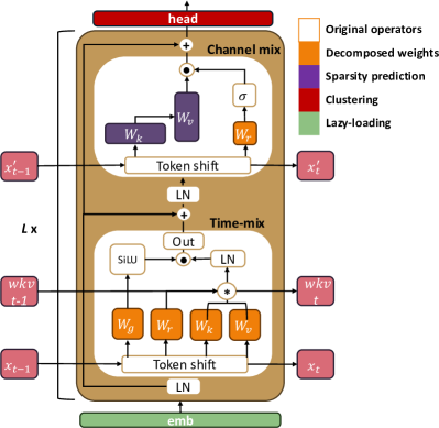
Figure 1: Simplified architecture of the RWKV model. Each variant has multiple ($L$) numbers of RWKV blocks, which comprise time and channel-mix layers. Colored blocks are our techniques onto the original layers. (LN=Layer Normalization).

Table 1: RWKV hyperparameters and parameter distribution of RWKV models. Each block scales differently in proportion to the model size, which guides where to optimize them.

3.1 RWKV

RWKV models are a family of RNN-based LLMs. Just like transformer-based LLMs, each RWKV model includes an embedding layer at the bottom (near the input), and a classification head at the top (near the output). Unlike transformers, between the embedding and the header are a stack of RWKV blocks (e.g. 12 or 24), each of which consists of a channel-mixing and a time-mixing layer (which are often referred to as “Attention (attn)” and “Feed-Forward Network (FFN)” for convenience). As depicted in Figure 1: RWKV blocks eschew attention mechanisms; rather, the state information propagates across timesteps as small, fixed-size vectors (e.g. $wkv_{t-1}$ or $wkv_{t}$ elements). Specifically, channel-mixing layers take the role of short-term memory to store the state of the previous information, while time-mixing layers act as long-term memory to retain a part of the previous states over a longer period. Inside RWKV blocks, the majority of weights are in the projection matrices termed as Receptance, Weight, Key, and Value, which are analogous to (but functionally different from) the Query, Key, and Value weights of Transformers.

3.2 Analysis of RWKV for potential optimization

Overall parameter distribution

RWKV models, depending on their variants, have different weight distribution across layers. Overall, the size of RWKV blocks scale quadractically with dimension $D$ and the number of blocks $L$. Depending on the block configuration, each block has a size of either $W\in\mathbb{R}^{D\times D}$ or $W\in\mathbb{R}^{D\times 3.5D}$. Note that the above description is about parameter scaling, not computational scaling. By comparison, Each of the embedding and the head layer is a $M\in\mathbb{R}^{D\times V}$ matrix; where $V$ is the vocabulary size. Embedding layer is a lookup table given a token index, and head layer is a linear layer to project the hidden state to a distribution over the vocabulary. Their sizes only scale with $D$ but not with number of RWKV blocks. As denoted in Table 1, for smaller models (tiny and small), the embedding and head layers occupy almost a half or third of the parameter sizes; such a fraction diminishes to about 15% for the medium model, for which the RWKV blocks dominate.

This suggests that: for smaller models, compressing the embedding and head layers would be as important as compressing the RWKV blocks; whereas for larger models, compressing embedding and head will yield marginal benefit. This observation guides us for navigating through tradeoffs between model size for accuracy, as Section 6.4.

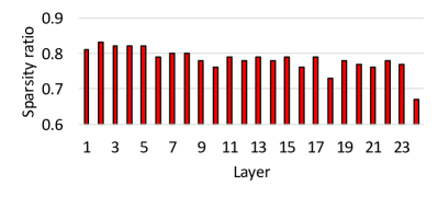
Figure 2: Average FFN’s sparsity ratio of 200 token generations in the channel-mix layer of the small (0.4B) RWKV model. Sparsity ratio refers to the rate of non-zero values in activations. Every layer has high sparsity, implying loading unnecessary weight row/columns.

Parameters in RWKV blocks

The RWKV weights are dominated by two groups of weight matrices: (1) several square matrices $W\in\mathbb{R}^{D\times D}$ in channel mix and time mix; they constitute 22% — 39% of total model weights, across different model sizes; (2) two FFN matrices for FFN $W\in\mathbb{R}^{D\times 3.5D}$ in channel mix; they constitute 25% — 44% of total model weights. Both groups of weights are critical for the model performance, and they need to be compressed. The sizes of all other weights (small vectors) are negligible. This is summarized in Table 1

To compress square projection matrices, our approach is low-rank approximation. Our hypothesis is that the intrinsic rank of such projection is low, and can be approximated by the product of two much smaller matrices (one ’tall’ and one ’flat’). Such low-rank approximation has shown high efficacy in model compression (e.g. LoRA (Hu et al., 2021) for fine-tuning LLMs); however, it was unclear whether they will apply to RWKV, which has very different representation than transformers; it was also unclear what mechanism (and effort) would be needed to recover the accuracy lost by decomposition.

To compress FFN non-square matrices, our approach is to exploit sparsity. Note that the FFN matrices are unamendable to low-rank approximation, as they are not square (they already have relatively lower rank; we confirmed: further decomposition would not reduce much weight while quickly degrading accuracy). Our motivation for sparsity is the nonlinearity (squared ReLU) between the two FFN matrices, which suppresses negative neurons as zeros; as well as the lottery ticket hypothesis (Frankle & Carbin, 2019) that only a small subset of parameters is essential for each token generation. However, RWKV sparsity was never examined before (as far as we know), and a lottery ticket hypothesis was never tested on RWKV (especially smaller models) (Liu et al., 2023; Xue et al., 2024; Song et al., 2024c, b, a)

Our new findings validate the existence of sparsity in RWKV: that is, to generate a token, only a small fraction of neurons in the FFN activation vector have non-zero values; correspondingly, only a small fraction of rows/columns in the FFN weight matrices participate in the computation effectively, and only these rows/columns need to be loaded in memory for this token. Figure 2 shows the sparsity of the RWKV’s FFN weight matrices across layers, ranging from 83% (bottom layers) to 67% (top layers).

To exploit the sparsity for memory saving, however, requires us to predict activated neurons without actually computing them. This raises significant, new challenges. (1) The RWKV sparsity level (–83%) is notably lower than large transformers (e.g. reported to be 99% in OPT-175B), which most prior work focused on (Liu et al., 2023). This not only means the ”headroom” for memory reduction is lower than large transformers, but also means that finding actually activated neurons is more difficult. False positives in predicting activated neurons would result in loading unnecessary weights, quickly diminishing the saving; false negatives would miss actually activated neurons that are key to model inference – leading to accuracy collapse. (2) As we focus on smaller models, the memory overhead of predictors themselves (often smaller neural networks) becomes non-negligible; the overhead of predictors could totally diminish the benefit of sparsity. These challenges combined, sparsity predictors known effective for transformers will fail for RWKV, as we will show in Section 4.2.

4 RWKV-edge: Deeply compressed RWKV

We present RWKV-edge, applying multiple techniques to reduce in-memory footprint, as demonstrated in Figure 1. We keep the original model shape and augment a few auxiliary layers to prevent performance drops incurred by our heavy compression.

4.1 Singular Vector Decomposition for RWKV blocks

Given a weight matrix $W\in\mathbb{R}^{M\times M}$, where $M$ is the embedding size, we apply two alternative methods with SVD Equation (10) to cover different use cases:

(1) Continual pretraining: given input data $X\in\mathbb{R}^{1\times M}$, computation for a single linear layer is represented as follows:

$$XW\approx(XL)R$$ (1)

where $L\in\mathbb{R}^{M\times(M/k)}$, $R\in\mathbb{R}^{(M/k)\times M}$, and $k$ is a compression factor e.g., $k=8$, which involves retaining only the top $M/k$ singular values. The computation equation can be implemented with two linear layers, referring to Equation (10): $L$ is a weight matrix $U\Sigma$, which has $M^{2}/k$ parameters. 2) $R$ is a weight matrix $V$, having also $M^{2}/k$ parameters.

We apply this equation to the vanilla pretrained model by (1) decomposing the original model and (2) continuing training with the decomposed version. The rational of such method is two folds: (1) dimensionality reduction from $M^{2}$ to $2M^{2}/k$ and (2) simplicity, achieved with two minimal layers that minimally disturbs the original weights. However, due to the minimal complexity, its performance degrades when non-linearity arises. Note that this training is pretraining, not fine-tuning; fine-tuning is specific to downstream tasks, which is not the focus here.

(2) Regular pretraining: to overcome the limitation of Equation (1), an enhanced computation for a single linear layer is formulated as below:

$$XW\approx relu(XL)^{2}R+(XD)$$ (2)

where $relu()$ is the activation function, and $D$ is a diagonal matrix containing singular values. We use the equation for pretraining from scratch. The rationale for introducing additional complexity is that such pretraining provides high flexibility in defining model architecture; therefore, we incorporate these new terms to improve expressiveness and approximation. In specific, the non-linearity magnifies differences between features by amplifying important activations and suppressing irrelevant ones, i.e., increasing model capacity. The diagonal matrix adjusts an approximated weight matrix, compensating for the rank reduction caused by SVD.

Note that augmented terms do not incur computational overheads much. For instance, the activation function and the diagonal matrix requires element-wise multiplication, which is $O(M)$; therefore, while the absolute GFLOPs are slightly higher than the original architecture, its cost is negligible. Since many edge CPUs support SIMD instructions, which can accelerate such computations, inference on our models incurs a trivial overhead.

Whichever method is used, we apply this exclusively to square matrices: $W_{r,k,v,g}$ in a time-mix layer, and $W_{r}$ in a channel-mix layer, as depicted in Figure 1. We do not apply $W_{o}$ in the time-mix, as this leads to detrimental effects due to its high-rank structure. When extending this method to non-square matrices, such as $W_{k,v}$ in the channel-mix, we observe that a mismatch between input and output dimensions of the matrices reduces the effectiveness of SVD, limiting the ability to express the most significant patterns in the weight e.g., overfitting or poor generalization.

4.2 Leveraging sparsity for lightweight FFNs in channel-mix layer

For non-square matrices such as FFN $W_{k,v}$ in the channel-mix, we utilize sparsity to reduce the memory footprint during inference, instead of employing SVD. Our first approach involves a set of small layers predicting the likely weight columns needed for a given input, which has been explored in other line of work (Xue et al., 2024; Liu et al., 2023); however, none have applied sparsity to RWKV models.

Given an input $X\in\mathbb{R}^{1\times M}$, the computation is defined by the following equation:

$$XW\approx\sigma(L_{2}(ReLU(XL_{1}))$$ (3)

where $L_{1}\in\mathbb{R}^{M\times N}$, $L_{2}\in\mathbb{R}^{N\times M}$, and $N$ is a hidden dimension for a linear layer. $\sigma$ represents the sigmoid activation function.

While these trained predictors (MLP predictors) perform well on transformer-based models, we found that they bring limited practical benefits on RWKV models, often dropping model accuracy. Because of this issue, we explore a unique and lightweight quantization such as 1/2/4 bits for sparsity prediction. The rationale of this approach is that quantization often preserves critical values despite introducing significant numerical errors.

Interestingly, we find that applying standalone–whether train-based or quantized predictors–can fail to capture essential weight columns. Notably, we observe that the quantized predictors generally outperform MLP predictors in predicting sparsity; yet, MLP predictors often retrieves valuable outliers, missed by the quantized version. Based on this observation, we adopt an ensemble predictor that combines both predictors to improve accuracy. The effectiveness of each predictor type and the benefits of the ensemble approach will be tackled in our evaluations.

4.3 Eliminating redundancy on outer layers

Although both head and embedding layers take less amount of parameters than the RWKV blocks, they still account for a significant portion of small RWKV models. We further squeeze the RWKV models to reach the least size, but performant models to work on resource-constrained environments. To do this, the key idea is to load only relevant tokens or corresponding embeddings during inference.

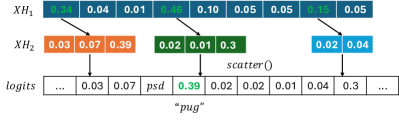
Figure 3: An illustration of the clustered heed. The clustered head loads only the few of high probable layers as their total probabilities exceed a predefined threshold, and then scatters their logits. psd refers to a pseudo-logit that covers unloaded logits.

Clustered head layer

We, first, apply the centroid-based clustering, such as KMeans, to word embeddings based on their similarity. After clustering, we re-train our decomposed models with our newly added cluster layers.

Given an input $X\in\mathbb{R}^{1\times M}$, the computation for the clustered head is denoted as follows:

$$C=cumsum(softmax(XH_{1}))$$ (4)

$$k_{cutoff}=min\{k:C[k]\geq p_{min}\}$$ (5)

$$k_{cutoff}=max(k_{min},min(k_{cutoff},k_{max}))$$ (6)

$$logits=XW\approx H_{2}Clusters[k_{cutoff}]$$ (7)

where $H_{1}\in\mathbb{R}^{M\times c}$ and $H_{2}\in\mathbb{R}^{M\times t}$. $c$ is the number of clusters and $t$ represents the number of tokens within each cluster. The clustered computation involves two layers: $H_{1}$ projects them embedding dimension $M$ to probabilities for $c$ clusters, and $H_{2}$ contains token embeddings for each cluster. The operation is visualized in Figure 3 and described as follows: the logit vector is initialized as $inf$. Equation (4, 5) identifies probable clusters by accumulating their probability until exceeding a predefined threshold $p_{min}$ e.g., 0.95. Equation (5, 6) extracts their cluster indices, and Equation (7) scatters the logits by multiplying the corresponding token embeddings $H_{2}$ and selected clusters. The token with the highest probability in the logit vector is then selected as the next token for generation.

While updating only logits of the most probable token loaded by the selected clusters preserves accuracy, this harms perplexity due to the absence of logits from unloaded clusters. This occurs because the calculation of perplexity depends on the complete probability distribution, which our initial method cannot fully capture.

To address this logit error, we apply pseudo-logits by utilizing the probability invariant e.g., $\Sigma^{k}_{i=0}P_{i}=1$. For instance, assume that there are unknown 50 logits among 100 of them. To approximate unknown logits, we leverage the relationship between the sum of softmax probabilities and exponentials:

$$P_{known}=\frac{logits_{known}}{logits_{known}+logits_{unknown}}$$ (8)

$$logits_{unknown}=logits_{known}\frac{1-P_{known}}{P_{known}}$$ (9)

Here, Equation (8) represents the softmax equation, and Equation (9) is its derived form. By calculating the derived form, we can determine the sum of unknown logits and distribute pseudo-logits by dividing this sum by the number of unknown logits.

Nevertheless, there is a caveat: while the pseudo-logit does recover perplexity, its calculation is non-trivial. This is because the operation requires iterating the unloaded clusters; hence, it should be used with caution, depending on its purpose of application–either perplexity or inference time.

Lazy embedding layer

We employ a caching mechanism for our embedding layer that loads only new tokens while reusing previously loaded ones. To manage a cache capacity, we set a threshold (e.g., 1000 tokens). Once the number of loaded embeddings are exceeded the threshold, the cache evicts the oldest token sequentially to make room for new tokens. We admit that this type of mechanism is not new and normally explored in Retrieval Augmented Generation (RAG) area. For example, the recent work (Jin et al., 2024) stores input embeddings to accelerate retrieval processing and reducing memory costs. This work deals with massive information to cover plenty words; on the contrary, ours tackles a small subset of words to process general text generation.

5 Implementation

Training details To pretrain our models, we use the Pile dataset (Gao et al., 2020) to train the baselines. Specifically, we use 200B tokens. This dataset is the largest that we can afford (given our limited academic resource budget) to train the models.

We have trained our models by regularly submitting jobs to a SLURM cluster at the authors’ institution. Each training job runs for at most 3 days (cluster policy) and on 4–6 A100 GPUs. As of this writing, we have trained ours models with 215B and 196B for the small and medium models.

How SVD is trained We utilized the Pile dataset to train our models for appropriate cases. For continual pretrain, we inherited the official checkpoints and modify their layers by applying Eq 1. For regular pretrain, we initialized models from scratch using random weights and biases, following Eq 2. This training requires the end-to-end training; hence, the most time-consuming.

How sparsity predictors are trained We trained sparsity predictors based on our pretrained models infused with our techniques. We recorded activations and accompanying weights by inputting multiple training samples. Using with them, we trained linear layers specific to the channel mix layer Unlike the SVD training, this approach does not require the end-to-end training. This is a similar approach to the existing work (Liu et al., 2023; Xue et al., 2024).

How head is trained We used our pretrained models with the Pile dataset. Since only the clustered head layer needs training, such as the time and channel mix layers, were frozen. Despite involving relatively few parameters, training the head layer requires end-to-end training because the layer resides at the final stage of the model.

Custom NEON kernels We put effort into making RWKV work on a variety of embedded devices by combining various optimizations, both existing and proposed by us. The original RWKV codebase only provides INT8 quantizations for CUDA kernels and defaults to Python’s tensor data type conversions for ARM CPUs, resulting in more than a 10x slowdown when quantized (INT8) RWKV inference runs on ARM CPUs. To address this, we implemented custom NEON kernels for fused dequantized and matrix-vector multiplications. To support a variety of ARM devices, our kernels include versions that dequantize to FP16 for chips supporting hardware NEON FP16 instructions (e.g., RPi5) and versions that dequantize to FP32 for chips that do not support FP16 (e.g., RPi4 and earlier, Opi).

Only via these NEON kernels does our evaluation (and demonstration) on INT8 become feasible on popular ARM devices such as RPi5. We will contribute them to the upstream RWKV codebase.

6 Experiments

We conduct a comprehensive evaluation of RWKV-edge to assess its performance, focusing on the following aspects: (1) accuracy, (2) memory usage, and (3) inference.

6.1 Methodology

Benchmarks.

We evaluate our models and systems on a wide range of benchmarks, details of which are provided in Appendix A. In this section, we focus on presenting the results of one benchmark: lambada_openai (Paperno et al., 2016), which we find to be the most challenging, comprising test cases such as long-range contextual and semantic reasoning. This benchmark is where most models encounter the most difficulty. On other easier benchmarks, the advantages of our models are even more pronounced (see Appendix for details).

Table 2: Models used in the experiments. ”Params” means the size of a checkpoint saved on disk, which differs from the memory usage.

Table 3: CPU platforms to test the model inference.

Model versions and baselines.

We consider a variety of RWKV models that are appropriate for edge (or resource constrained) devices that RWKV were designed for. Table 6 listed these variants as well as their hyperparametres. Specifically, we compare the following implementations.

• RWKV-vanilla: the RWKV (v5) checkpoints released by the authors; unmodified.

• RWKV-ours: we take RWKV-vanilla, modify their architectures to ours, and continue to pre-train the models on the aforementioned Pile dataset (not any specific downstream tasks). We update all the model parameters as we want the altered models to recover their accuracy; empirically, we find that frozen model parts result in inferior accuracy.

We further compare to the following transformer models of similar sizes and FLOPs requirements (also listed in Table 6): OPT (Zhang et al., 2022), GPT-Neo (Black et al., 2021), and smaller variants of Llama (Miao et al., 2024; mic, ; Zhang et al., 2024).

Inference.

We execute inference with FP16 and INT8 and apply the optimal thresholds for our techniques to our models. For instance, we use the ensemble predictors and appropriate thresholds for them, depending on the model size. For a metric, we use token-per-second (TPS), which is a typical performance metric for text generation. To verify our effective models, we deploy them and measure their performance on two edge platforms, listed in Table 3.

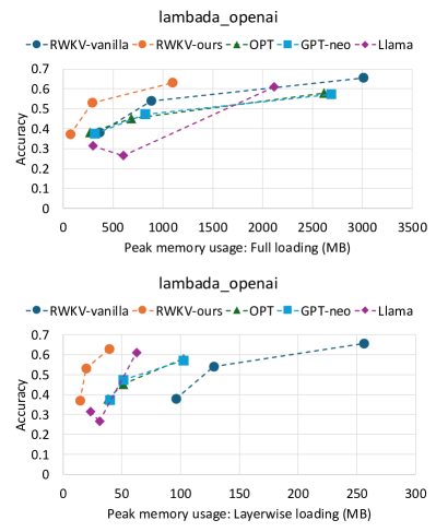
Figure 4: Accuracy & memory footprint comparison between RWKV and transformer models. RWKV-ours has smaller memory footprint than other models and still maintain the comparable accuracy on both loading strategies. All models are FP16.

6.2 Model Memory footprint

We consider a model’s memory footprint as its maximum memory usage during model inference. Results in Figure 4 show that we significantly reduce memory footprint, while incurring little or no reduction in the inference accuracy that is defined by the benchmark tasks, e.g., accuracy defined in a word prediction task. Our techniques also preserve model perplexity, which measures the model output fluency or coherence; see Appendix A for details.

We characterize a model’s memory footprint under popular model loading strategies: (1) full loading: a mainstream approach adopted by ML inference on the edge: as the inference code launches, it loads all the model parameters into the memory, and therefore avoids any disk IO at inference time; with our techniques, full loading would load all the weights except those in embedding, FFNs (in channel-mix), and classification head, which are managed by our proposed techniques in Section 4.2–4.3. (2) layerwise loading: an approach for more aggressive memory reduction: the inference code loads layer N+1 while executing layer N; this shrinks the memory footprint but nevertheless incurs high delays in disk IO at inference time.

Figure 4 shows that RWKV-ours , compared to RWKV-vanilla , reduces the memory for full loading by 4x on average, and for layerwise loading by 5x on average. Meanwhile, RWKV-ours only experiences little accuracy drop, around 3.8pp and 4.9pp for small, and medium models, respectively.

Figure 5 further breaks down our memory footprint by model components. Across all model sizes, our techniques (SVD and sparsity) significantly reduce the memory footprint of RWKV blocks, by 2.5x for the time-mix and 3.6x for the channel-mix. In particular, for tiny and small models where the embedding and head layers are major memory consumers, our clustered head reduces memory usage by 6.7x by loading only relevant weight clusters for predicted output tokens, and our embedding cache reduces memory by more than an order of magnitude by only loading embeddings for tokens in the context. Without these two optimizations (and only with SVD and sparsity), we would not see much memory reduction for smaller models.

Comparison to Transformer models

Our RWKV models demonstrate a clear advantage against transformer models in terms of memory efficiency. Results are shown in Figure 4(a) and (b). Note that this comparison favors transformers by not counting their KV cache sizes; RWKV maintains compact, O(1) memory states across timesteps, and therefore does not require KV caches by design.

At similar accuracy levels, RWKV-ours consume 3x less memory than transformer models, as exemplified by our medium model (the rightmost ) vs. Llama (the right most ) in the figures. With similar memory footprints, RWKV-ours achieves much higher accuracy than transformers, as shown by RWKV-ours vs. GPT-neo or Llama in the figures. Much of the benefit comes from our techinques instead of RWKV itself: RWKV-vanilla, without our optimzations, would see lower or marginal memory savings, as shown by RWKV-vanilla vs. OPT or GPT-neo in the figures.

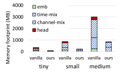
Figure 5: Breakdown of full loading on RWKV models. Our models have significant reduction in all components e.g., embedding, time/channel-mix, and head.

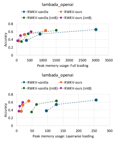
Figure 6: Comparison of accuracy and memory usage between float16 and int8 for RWKV models. Our models are complement to quantization without a significant performance drop.

Compatibility with quantization

Our optimizations complement model quantization effectively. Combined with a popular quantization scheme INT8, this results in a 10x reduction in memory footprint on average across different parameter sizes (of which 2x from quantization and around 5x from our optimizations).

To demonstrate this, we compare RWKV-vanilla and RWKV-ours, both before and after quantization. As shown in Figure 6, RWKV-ours benefits from INT8 quantization by reducing memory usage by roughly 2x while incurring minimal in accuracy (less than 1pp on both small and medium models). This indicates that RWKV-ours is as robust, if not more so, to quantization compared to RWKV-vanilla, which sees an average loss of 1.5pp across different parameter sizes.

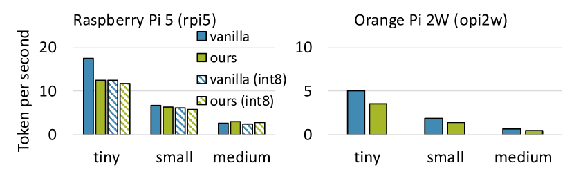
(a)

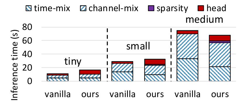
(b)

Figure 7: (a) Comparison of TPS between RWKV-vanilla and RWKV-ours on rpi5 and opi2w. RWKV-ours exhibits a slight loss, compared to RWKV-vanilla. This loss becomes minor in the small model. (b) Breakdown of RWKV-vanilla/ours inference time on rpi5. The head layer is the main difference between vanilla and ours; additionally, its layer becomes smaller on larger models while other layers remain the same.

6.3 Inference speed

Our memory optimization does not slow down inference much compared to RWKV-vanilla. As shown in Figure 7(a), running FP16 small and medium models, RWKV-ours see a slight TPS drop or no degradation (5% drop and 20% increase for each model); on tiny model, the drop is more noticeable (29%). The major factor of such slowdown, as illustrated in Figure 7(b), comes from the clustered head layer, which does gather-scatter operations on pseudo logits (lower parallelism, memory latency bound) in lieu of a full matrix multiplication (regular parallelism). As model sizes increase, the overhead of clustered head is dwarfed by those of RWKV blocks, diminishing the gap in inference speeds.

For INT8 inference, RWKV-ours and vanilla show similar inference speeds to the FP16 inference with minor TPS drops. Note that this is a remarkable achievement thanks to our NEON kernels; Turning off the kernels leads a detrimental effect on the speed (10x slower). As shown in Figure 7(a), all sizes from tiny to medium RWKV-ours show a minor decrease in TPS, which is 7%, 9%, and 5%, respectively. RWKV-vanillas show similar performance drops (10% and 9%) on small and medium models; on the contrary, running the tiny vanilla results in a drop in 40% TPS. These performance drops in INT8 compared to FP16 are due to under-optimization, e.g., cache alignment for a specific instruction. We will plan to close this gap in future work.

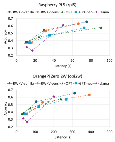
Figure 8: Model comparison between transformer and RWKV models on both CPU platforms. The model sizes are medium, small, and tiny from left to right. RWKV-ours are the optimal models among displayed models considering all crucial metrics e.g., accuracy, peak memory usage, and TPS.

Inference: Transformer vs. RWKV.

RWKV-ours have slight drops or no degradation in token-per-second (TPS) at similar accuracy levels, such as for medium and small models. While RWKV-vanilla has higher accuracy than any other models, its benefits in memory reduction and TPS are minor. As demonstrated in Figure 8, RWKV-ours results in 19% drops and 7% gains in TPS on average, compared to other small and medium transformer models on the rpi5; by contrast, executing our tiny model drops 28%. This is understandable because our models require more GFLOPs due to additional multiplications induced by our augmented layers. While RWKV-ours have little benefits on TPS, our models are more optimal other transformer models with a similar or higher accuracy and huge amount of memory savings. On the opi2w, we found that tendencies of the resultant numbers are very homogeneous to those of rpi5; therefore, we omit its description.

Energy consumption

RWKV-ours consume slightly more energy per inference, compared to RWKV-vanilla. As measured using a USB power meter, both variants, during active inference, draw the same device power (around 6.5 Watts for Rpi5). Hence, the total energy consumption is proportional to the time taken to generate a certain number of tokens, with RWKV-ours consuming approximately 10% more energy on the small models (e.g., 214J vs 195J for 200 tokens)

6.4 Ablation study

We conduct ablation study to evaluate individual effectiveness of each technique. For SVD, we apply $k=8$ factor to decompose the weight matrices; for the clustering and sparsity predictor, we set appropriate thresholds and bits for each model size to achieve the best accuracy.

Our optimizations impact on accuracy

As shown in Table 4, we observe that the ablated models show a slight drop in accuracy compared to RWKV-vanilla; The losses are 1.3pp, 0.7pp and 2pp from tiny, small and medium models, respectively; the numbers are averaged across ablated models in the same parameter sizes. Overall, among the three optimizations, SVD has the highest impact on model accuracy while Sparsity shows the least. Notably, the accuracy of the SVD-ablated models are closely aligned with the vanilla models. This is reasonable because ablating SVD essentially reverts the models to their vanilla counterparts. Considering that the memory efficiency from CLS diminishes as the model layers and dimensions scale up, we disable CLS for medium or larger models. For a detailed breakdown of individual memory efficiency, we refer to the contents presented in Figure 5.

Table 4: Accuracy of ablated models. Benchmark: OpenAI lambada. A component column refers to the model with all components except the specified component. Ablated models have slight drops in accuracy; yet, having more memory usage than full models (all). (SVD = Singular Value Decomposition, CLS = the clustered head, Sparse = sparsity predictors)

6.5 Sensitive analysis

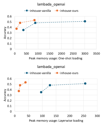
Figure 9: Accuracy & peak memory usage comparison of inhouse RWKV models. inhouse-ours has smaller memory footprint than inhouse-vanilla models and still maintain the comparable accuracy on both loading strategies.

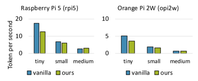
Figure 10: Comparison of TPS between inhouse-vanilla and inhouse-ours on rpi5 and opi2w. inhouse-ours exhibits a slight loss, compared to inhouse-vanilla. This loss becomes minor in the small model.

SVD as a suitable architecture for pretraining.

We test the idea, Eq 2, in section 4.1: replacing $W\in R^{D\times D}$ projection matrices with their SVD decomposition format, which is further enhanced with non-linearity, composed by full-rank, diagonal matrices. We initialize such a model architecture from scratch and pretrain them with the Pile datasets. We named these models, pretrained by us from scratch, as “in-house” checkpoints: inhouse-vanilla: models in the vanilla architecture without our optimiziations. inhouse-ours: model architectures with our optimizations.

As Figure 9 shows, the comparison between inhouse-vanilla and inhouse-ours manifests that the SVD can be a suitable choice. While reducing the parameters of project matrices by 4x (and the total model sizes by 4.8x–3.5x, ranging from tiny to medium models), the total accuracy sees, rather, slight gains: 1.4pp on average. The additional FLOPS required by SVD (at inference time) is also negligible: as shown in Figure 10, inhouse-ours is only 13.7% slower than inhouse-vanilla on average on rpi5, and 20% slower on opi2w. Furthermore, we observed little to none training throughput difference on these two inhouse-vanilla and inhouse-ours. This suggest that SVD should be considered as a “free” size optimization for pretraining RWKV models.

We notice an important caveat, though. inhouse-vanilla, with our trainig budget and datasets, fall under the accuracy of the official checkpoints (for instance, on lambada_openai, inhouse-vanilla show lower accuracy by 7.7pp from tiny to medium models. Full results are in the appendix. We attribute the reason as the official checkpoints were trained for far more tokens (1.12 T, 5x more than ours) and datasets (RWKV authors disclosed their choices of their training data, but not the exact ratios or scripts (Peng et al., 2023)).

The choice of low-rank approximation factors

We tested aggressive (16x) and light (4x) SVD decomposition factors to find the optimal balance between memory efficiency and accuracy. We find that the 16x factor results in detrimental accuracy; on the contrary, the light decomposition (4x) brings a slight or no accuracy improvement, compared to 8x default decomposition. In detail, 16x shows significant drops: 2.85pp for the tiny model, 11pp for the small model, and 29pp for the medium model; 4x models achieve very similar accuracy to 8x with less than 1pp. For the light decomposition, albeit comparable accuracy, it still provides complementary benefits with quantization regarding to memory efficiency.

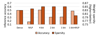
Figure 11: Accuracy and sparsity rate achieved by the ground-truth (GT) and quantized predictors ($n$-bit). Benchmark: lambada_openai

A variety of sparsity predictors

We find that a deeply quantized predictor (1-bit), when ensembled with a learning-based MLP, can provide the best of both worlds: small predictor size and high neuron recall. This combination outperforms using either the MLP or a larger quantized predictor (e.g., 4-bit) alone.

To show this, we study a range of sparsity predictors and their ensembles on our small model by executing inference for the OpenAI benchmark. As illustrated in Figure 11, n-bit quantized networks, which constitute 1/n of the original FP16 FFN size, can predict the sparsity rate and accuracy close to the ground truth (83% vs 85%), while aggressive quantized networks (1/2-bits) lose their accuracy by a half of that of 4-bit network despite their similar sparsity rate. However, we found that these accuracy losses from heavy quantization can be mitigated by ensembling the quantized predictor and MLP. Specifically, one such ensemble (1-bit and MLP) leads to losing minor accuracy degradation (1.7pp) and having less memory usage due to aggressive quantization, compared to the sole 4-bit quantized network. This indicates that the 4-bit predictor w/o MLP is more accurate, while the 1-bit predictor w/ MLP is more memory efficient, which suggests that the choice of predictor depends on the user’s priorities, whether favoring memory reduction or higher accuracy, and highlights the trade-off between these two factors.

The number of clusters

We find that applying appropriate thresholds for the clustered head is crucial to achieve the best accuracy and memory efficiency. To find out its implication, we varied its threshold to load more (0.99) or less (0.85) number of clusters; our default is 0.95, which is empricially determined at best. We observe that 0.85 reduces the memory usage by 2x, yet dropping 10pp in accuracy. Conversely, increasing the value to 0.99 loads 2x more clusters, which volumes the memory usage up by 2x; yet, this improves 1.5pp in accuracy. Note that the described memory usage is derived from only the clustered head size, not from the entire model. Our results implicate that the number of clusters should be carefully determined to balance the trade-off between the memory usage and the accuracy. Finally, we observe that the inference time is not much affected by the number of clusters.

7 Conclusions

In this study, we present RWKV-edge, a suite of efficient compression techniques for RWKV models, which are easily deployable and runnable on edge devices such as Raspberry Pi 5. RWKV-edge primarily incorporates SVD, ensemble sparsity predictors, and clustered head. By applying those compressing techniques, RWKV models can achieve a reduction of 4.95x–3.8x in memory usage while losing only 2.95pp in accuracy compared to the vanilla models. Although RWKV-edge introduces computational overheads, we demonstrate that these overheads are negligible for deployment on edge devices.

Appendix A Additional evaluation

We report our full evaluations on the official and our models here.

Table 5: A collection of benchmark tasks for the model evaluation. Tasks are popularly used in the LLM evaluation.

Table 6: Benchmark results for all models (acc = accuracy, ppl = perplexity).

Appendix B Background

Singular Value Decomposition (SVD)

SVD is one of the low-rank factorizations to approximate an original weight matrix with standard factorization. It decomposes the matrix into three matrices ($U,\Sigma,V$) and multiplies them to approximate the original one with fewer total parameters.

Given a matrix $W\in\mathbb{R}^{M\times N}$, SVD reconstructs it as follows:

$$W\approx U\Sigma V^{T}$$ (10)

where $U\in\mathbb{R}^{M\times r}$, $V\in\mathbb{R}^{N\times r}$, and $r$ is a target rank for SVD. $\Sigma$ is a diagonal matrix of non-zero singular values $diag(\sigma_{1},...,\sigma_{r})$, where $\sigma_{1}\geq\sigma_{2}\geq...\geq\sigma_{r}\geq...\geq\sigma_{k}>0$, and $k$ is the rank of matrix $W$. Setting zeros to $\sigma_{r+1},...,\sigma_{k}$ achieves the low-rank approximation.

References

- (1) rwkv.cpp. https://github.com/RWKV/rwkv.cpp. [Accessed 26-09-2024].
- (2) Microllama. https://github.com/keeeeenw/MicroLlama.
- Acharya et al. (2018) Acharya, A., Goel, R., Metallinou, A., and Dhillon, I. Online Embedding Compression for Text Classification using Low Rank Matrix Factorization, November 2018.
- (4) Agarwal, S., Acun, B., Hosmer, B., Elhoushi, M., Lee, Y., Venkataraman, S., Papailiopoulos, D., and Wu, C.-J. CHAI: Clustered Head Attention for Efficient LLM Inference.
- Barnabò et al. (2023) Barnabò, G., Uva, A., Pollastrini, S., Rubagotti, C., and Bernardi, D. Supervised Clustering Loss for Clustering-Friendly Sentence Embeddings: An Application to Intent Clustering. In Findings of the Association for Computational Linguistics: IJCNLP-AACL 2023 (Findings), pp. 412–430, Nusa Dua, Bali, 2023. Association for Computational Linguistics. doi: 10.18653/v1/2023.findings-ijcnlp.36.
- Ben Noach & Goldberg (2020) Ben Noach, M. and Goldberg, Y. Compressing Pre-trained Language Models by Matrix Decomposition. In Wong, K.-F., Knight, K., and Wu, H. (eds.), Proceedings of the 1st Conference of the Asia-Pacific Chapter of the Association for Computational Linguistics and the 10th International Joint Conference on Natural Language Processing, pp. 884–889, Suzhou, China, December 2020. Association for Computational Linguistics. doi: 10.18653/v1/2020.aacl-main.88.
- Black et al. (2021) Black, S., Gao, L., Wang, P., Leahy, C., and Biderman, S. GPT-Neo: Large Scale Autoregressive Language Modeling with Mesh-Tensorflow, March 2021. URL https://doi.org/10.5281/zenodo.5297715. If you use this software, please cite it using these metadata.
- Chen et al. (2018) Chen, P. H., Si, S., Li, Y., Chelba, C., and Hsieh, C.-j. GroupReduce: Block-Wise Low-Rank Approximation for Neural Language Model Shrinking, June 2018.
- (9) Coda-Forno, J., Binz, M., Akata, Z., Botvinick, M., Wang, J. X., and Schulz, E. Meta-in-context learning in large language models.
- Dettmers & Zettlemoyer (2023) Dettmers, T. and Zettlemoyer, L. The case for 4-bit precision: K-bit Inference Scaling Laws. In Proceedings of the 40th International Conference on Machine Learning, pp. 7750–7774. PMLR, July 2023.
- Frankle & Carbin (2019) Frankle, J. and Carbin, M. The Lottery Ticket Hypothesis: Finding Sparse, Trainable Neural Networks, March 2019.
- Frantar et al. (2023) Frantar, E., Ashkboos, S., Hoefler, T., and Alistarh, D. GPTQ: Accurate Post-Training Quantization for Generative Pre-trained Transformers, March 2023.
- Gao et al. (2020) Gao, L., Biderman, S., Black, S., Golding, L., Hoppe, T., Foster, C., Phang, J., He, H., Thite, A., Nabeshima, N., Presser, S., and Leahy, C. The Pile: An 800gb dataset of diverse text for language modeling. arXiv preprint arXiv:2101.00027, 2020.
- Hsu et al. (2022) Hsu, Y.-C., Hua, T., Chang, S.-E., Lou, Q., Shen, Y., and Jin, H. LANGUAGE MODEL COMPRESSION WITH WEIGHTED LOW-RANK FACTORIZATION. 2022.
- Hu et al. (2021) Hu, E. J., Shen, Y., Wallis, P., Allen-Zhu, Z., Li, Y., Wang, S., Wang, L., and Chen, W. LoRA: Low-Rank Adaptation of Large Language Models, October 2021.
- Jin et al. (2024) Jin, C., Zhang, Z., Jiang, X., Liu, F., Liu, X., Liu, X., and Jin, X. RAGCache: Efficient Knowledge Caching for Retrieval-Augmented Generation, April 2024.
- Liu et al. (2023) Liu, Z., Wang, J., Dao, T., Zhou, T., Yuan, B., Song, Z., Shrivastava, A., Zhang, C., Tian, Y., Re, C., and Chen, B. Deja Vu: Contextual Sparsity for Efficient LLMs at Inference Time, October 2023.
- Miao et al. (2024) Miao, X., Oliaro, G., Zhang, Z., Cheng, X., Wang, Z., Zhang, Z., Wong, R. Y. Y., Zhu, A., Yang, L., Shi, X., Shi, C., Chen, Z., Arfeen, D., Abhyankar, R., and Jia, Z. SpecInfer: Accelerating Large Language Model Serving with Tree-based Speculative Inference and Verification. In Proceedings of the 29th ACM International Conference on Architectural Support for Programming Languages and Operating Systems, Volume 3, volume 3 of ASPLOS ’24, pp. 932–949, New York, NY, USA, April 2024. Association for Computing Machinery. ISBN 9798400703867. doi: 10.1145/3620666.3651335.
- Paperno et al. (2016) Paperno, D., Kruszewski, G., Lazaridou, A., Pham, Q. N., Bernardi, R., Pezzelle, S., Baroni, M., Boleda, G., and Fernández, R. The LAMBADA dataset: Word prediction requiring a broad discourse context, June 2016.
- Peng et al. (2023) Peng, B., Alcaide, E., Anthony, Q., Albalak, A., Arcadinho, S., Biderman, S., Cao, H., Cheng, X., Chung, M., Grella, M., GV, K. K., He, X., Hou, H., Lin, J., Kazienko, P., Kocon, J., Kong, J., Koptyra, B., Lau, H., Mantri, K. S. I., Mom, F., Saito, A., Song, G., Tang, X., Wang, B., Wind, J. S., Wozniak, S., Zhang, R., Zhang, Z., Zhao, Q., Zhou, P., Zhou, Q., Zhu, J., and Zhu, R.-J. RWKV: Reinventing RNNs for the Transformer Era, December 2023.
- Peng et al. (2024) Peng, B., Goldstein, D., Anthony, Q., Albalak, A., Alcaide, E., Biderman, S., Cheah, E., Du, X., Ferdinan, T., Hou, H., Kazienko, P., GV, K. K., Kocoń, J., Koptyra, B., Krishna, S., McClelland Jr., R., Muennighoff, N., Obeid, F., Saito, A., Song, G., Tu, H., Woźniak, S., Zhang, R., Zhao, B., Zhao, Q., Zhou, P., Zhu, J., and Zhu, R.-J. Eagle and Finch: RWKV with Matrix-Valued States and Dynamic Recurrence, April 2024.
- Sherstinsky (2020) Sherstinsky, A. Fundamentals of Recurrent Neural Network (RNN) and Long Short-Term Memory (LSTM) network. Physica D: Nonlinear Phenomena, 404:132306, March 2020. ISSN 01672789. doi: 10.1016/j.physd.2019.132306.
- Song et al. (2024a) Song, C., Han, X., Zhang, Z., Hu, S., Shi, X., Li, K., Chen, C., Liu, Z., Li, G., Yang, T., and Sun, M. ProSparse: Introducing and Enhancing Intrinsic Activation Sparsity within Large Language Models, July 2024a.
- Song et al. (2024b) Song, Y., Mi, Z., Xie, H., and Chen, H. PowerInfer: Fast Large Language Model Serving with a Consumer-grade GPU. In Proceedings of the ACM SIGOPS 30th Symposium on Operating Systems Principles, pp. 590–606, Austin TX USA, November 2024b. ACM. ISBN 9798400712517. doi: 10.1145/3694715.3695964.
- Song et al. (2024c) Song, Y., Xie, H., Zhang, Z., Wen, B., Ma, L., Mi, Z., and Chen, H. Turbo Sparse: Achieving LLM SOTA Performance with Minimal Activated Parameters, June 2024c.
- Tipirneni et al. (2024) Tipirneni, S., Adkathimar, R., Choudhary, N., Hiranandani, G., Amjad, R. A., Ioannidis, V. N., Yuan, C., and Reddy, C. K. Context-Aware Clustering using Large Language Models, May 2024.
- Viswanathan et al. (2024) Viswanathan, V., Gashteovski, K., Gashteovski, K., Lawrence, C., Wu, T., and Neubig, G. Large Language Models Enable Few-Shot Clustering. Transactions of the Association for Computational Linguistics, 12:321–333, 2024. doi: 10.1162/tacl˙a˙00648.
- Xue et al. (2024) Xue, Z., Song, Y., Mi, Z., Chen, L., Xia, Y., and Chen, H. PowerInfer-2: Fast Large Language Model Inference on a Smartphone, June 2024.
- Zhang et al. (2024) Zhang, P., Zeng, G., Wang, T., and Lu, W. Tinyllama: An open-source small language model, 2024.
- Zhang et al. (2022) Zhang, S., Roller, S., Goyal, N., Artetxe, M., Chen, M., Chen, S., Dewan, C., Diab, M., Li, X., Lin, X. V., Mihaylov, T., Ott, M., Shleifer, S., Shuster, K., Simig, D., Koura, P. S., Sridhar, A., Wang, T., and Zettlemoyer, L. OPT: Open Pre-trained Transformer Language Models, June 2022.