Fast and Robust
Visuomotor Riemannian Flow Matching Policy

Abstract

Diffusion-based visuomotor policies excel at learning complex robotic tasks by effectively combining visual data with high-dimensional, multi-modal action distributions. However, diffusion models often suffer from slow inference due to costly denoising processes or require complex sequential training arising from recent distilling approaches. This paper introduces Riemannian Flow Matching Policy (RFMP), a model that inherits the easy training and fast inference capabilities of flow matching (FM). Moreover, RFMP inherently incorporates geometric constraints commonly found in realistic robotic applications, as the robot state resides on a Riemannian manifold. To enhance the robustness of RFMP, we propose Stable RFMP (SRFMP), which leverages LaSalle’s invariance principle to equip the dynamics of FM with stability to the support of a target Riemannian distribution. Rigorous evaluation on eight simulated and real-world tasks show that RFMP successfully learns and synthesizes complex sensorimotor policies on Euclidean and Riemannian spaces with efficient training and inference phases, outperforming Diffusion Policies while remaining competitive with Consistency Policies.

I Introduction

Deep generative models are revolutionizing robot skill learning due to their ability to handle high-dimensional multimodal action distributions and interface them with perception networks, enabling robots to learn sophisticated sensorimotor policies [1]. In particular, diffusion-based models such as diffusion policies (DP) [2, 3, 4, 5, 6, 7] exhibit exceptional performance in imitation learning for a large variety of simulated and real-world robotic tasks, demonstrating a superior ability to learn multimodal action distributions compared to previous behavior cloning methods [8, 9, 10]. Nevertheless, these models are characterized by an expensive inference process as they often require to solve a stochastic differential equation, thus hindering their use in certain robotic settings [11], e.g., for highly reactive motion policies.

For instance, DP [2], typically based on a Denoising Diffusion Probabilistic Model (DDPM) [12], requires approximately $100$ denoising steps to generate an action. This translates to roughly $1$ second on a standard GPU. Even faster approaches such as Denoising Diffusion Implicit Models (DDIM) [13], still need $10$ denoising steps, i.e., $0.1$ second, per action [2]. Consistency policy [3] aims to accelerate the inference process by training a student model to mimic a DP teacher with larger denoising steps. Despite providing a more computationally-efficient inference, the CP training requires more computational resources and might be unstable due to the sequential training of the two models. Importantly, training these models becomes more computationally demanding when manipulating data with geometric constraints, e.g., robot end-effector orientations, as the computation of the score function of the diffusion process is not as simple as in the Euclidean case [14]. Furthermore, the inference process also incurs increasing computational complexity.

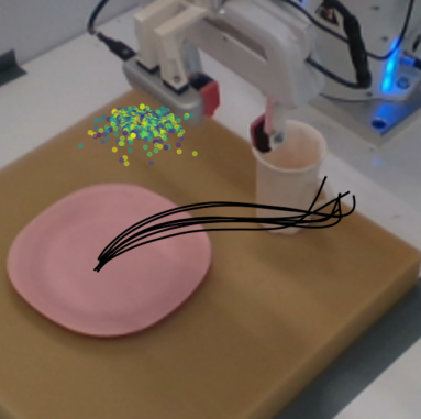
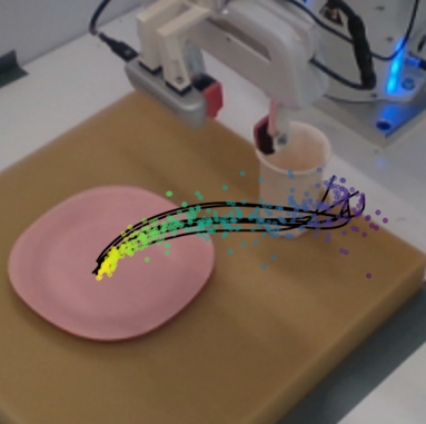
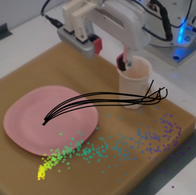
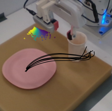
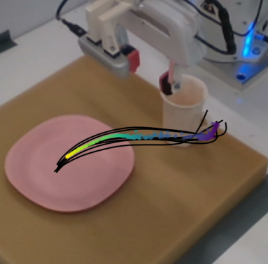
Figure 1: Flows of the RFMP (top) and SRFMP (bottom) at times $t=\{0.0,1.0,1.5\}$. The policies are learned from pick-and-place demonstration (black) and conditioned on visual observations. Note that the flow of SRFMP is stable to the target distribution at $t>1.0$, enhancing the policy robustness and inference time.

To overcome these limitations, we propose to learn visuomotor robot skills via a Riemannian flow matching policy (RFMP). Compared to DP, RFMP builds on another kind of generative model: Flow Matching (FM) [15, 16]. Intuitively, FM gradually transforms a simple prior distribution into a complex target distribution via a vector field, which is represented by a simple function. The beauty of FM lies in its simplicity, as the resulting flow, defined by an ordinary differential equation (ODE), is much easier to train and much faster to evaluate compared to the stochastic differential equations of diffusion models. However, as many visuomotor policies are represented in the robot’s operational space, action representations must include both end-effector position and orientation. Thus, the policy must consider that orientations lie on either the $\mathcal{S}^{3}$ hypersphere or the $\operatorname{SO}(3)$ Lie group, depending on the specific parametrization. To properly handle such data, we leverage Riemannian flow matching (RFM) [16], an extension of flow matching that accounts for the geometric constraints of data lying on Riemannian manifolds. In our previous work [17], we introduced the idea of leveraging flow matching in robot imitation learning and presented RFMP, which capitalizes on the easy training and fast inference of FM methods to learn and synthesize end-effector pose trajectories. However, our initial evaluation was limited to simple proof-of-concept experiments on the LASA dataset [18].

In this paper, we demonstrate the effectiveness of RFMP to learn complex real-world visuomotor policies and present a systematic evaluation of the performance of RFMP on both simulated and real-world manipulation tasks. Moreover, we propose Stable Riemannian Flow Matching Policy (SRFMP) to enhance the robustness of RFMP (see Figure 1). SRFMP builds on stable flow matching (SFM) [19, 20], which leverages LaSalle’s invariance principle [21] to equip the dynamics of FM with stability to the support of the target distribution. Unlike SFM, which is limited to Euclidean spaces, SRFMP generalizes this concept to Riemannian manifolds, guaranteeing the stability of the RFM dynamics to the support of a Riemannian target distribution. We systematically evaluate RFMP and SRFMP across $8$ tasks in both simulation and real-world settings, with policies conditioned on both state and visual observations. Our experiments demonstrate that RFMP and SRFMP inherit the advantages from FM models, achieving comparable performance to DP with fewer evaluation steps (i.e., faster inference) and significantly shorter training times. Moreover, our models achieve competitive performance compared to CP [3] on several simulated tasks. Notably, SRFMP requires fewer ODE steps than RFMP to achieve an equivalent performance, resulting in even faster inference times.

In summary, beyond demonstrating the effectiveness of our early work on simulated and real robotic tasks, the main contributions of this article are threefold: (1) We introduce Stable Riemannian Flow Matching (SRFM) as an extension of SFM [20] to incorporate stability into RFM; (2) We propose stable Riemannian flow matching policy (SRFMP), which combines the easy training and fast inference of RFMP with stability guarantees to Riemannian target action distribution; (3) We systematically evaluate both RFMP and SRFMP across $8$ tasks from simulated benchmarks and real settings. Supplementary material is available on the paper website https://sites.google.com/view/rfmp.

II Related work

As the literature on robot policy learning is arguably vast, we here focus on approaches that design robot policies based on flow-based generative models.

Normalizing Flows are arguably the first broadly-used generative models in robot policy learning [22]. They were commonly employed as diffeomorphisms for learning stable dynamical systems in Euclidean spaces [23, 24, 25], with extensions to Lie groups [26] and Riemannian manifolds [27], similarly addressed in this paper. The main drawback of normalizing flows is their slow training, as the associated ODE needs to be integrated to calculate the log-likelihood of the model. Moreover, none of the aforementioned works learned sensorimotor policies based on visual observations via imitation learning.

Diffusion Models [28] recently became state-of-art in imitation learning because of their ability to learn multi-modal and high-dimensional action distributions. They have been primarily employed to learn motion planners [29], and complex control policies [2, 30, 4]. Recent extensions consider to use 3D visual representations from sparse point clouds [6], and to employ equivariant networks for learning policies that, by design, are invariant to changes in scale, rotation, and translation [7]. However, a major drawback of diffusion models is their slow inference process. In [2], DP requires $10$ to $100$ denoising steps, i.e., $0.1$ to $1$ second on a standard GPU, to generate each action. Consistency models (CM) [31] arise as a potential solution to overcome this drawback [3, 32, 33]. CM distills a student model from a pretrained diffusion model (i.e., a teacher), enabling faster inference by establishing direct connections between points along the probability path. Nevertheless, this sequential training process increases the overall complexity and time of the whole training phase.

Flow Matching [15] essentially trains a normalizing flow by regressing a conditional vector field instead of maximizing the likelihood of the model, thus avoiding to simulate the ODE of the flow. This leads to a significantly simplified training procedure compared to classical normalizing flows. Moreover, FM builds on simpler probability transfer paths than diffusion models, thus facilitating faster inference. Tong et al. [34] showed that several types of FM models can be obtained according to the choice of conditional vector field and source distributions, some of them leading to straighter probability paths, which ultimately result in faster inference. Rectified flows [35] is a similar simulation-free approach that designs the vector field by regressing against straight-line paths, thus speeding up inference. Note that rectified flows are a special case of FM, in which a Dirac distribution is associated to the probability path [34]. Due to their easy training and fast inference, FM models quickly became one of the de-facto generative models in machine learning and have been employed in a plethora of different applications [36, 37, 38, 39, 40, 41].

In our previous work [17], we proposed to leverage RFM to learn sensorimotor robot policies represented by end-effector pose trajectories on Riemannian manifolds. Building on a similar idea, subsequent works have used FM along with an equivariant transformer to learn $\operatorname{SE}(3)$-equivariant policies [42], for multi-support manipulation tasks with a humanoid robot [43], and for point-cloud-based robot imitation learning [44]. In this paper, we build upon our previous work, Riemannian Flow Matching Policy (RFMP), to enable the learning of complex visuomotor policies on Riemannian manifolds. Unlike the aforementioned approaches, our work focuses on providing a fast and robust RFMP inference process. We achieve this by constructing the FM vector field using LaSalle’s invariance principle, which not only enhances inference robustness with stability guarantees but also preserves the easy training and fast inference capabilities of RFMP.

III Background

In this section, we provide a short background on Riemannian manifolds, and an overview of the flow matching framework with its extension to Riemannian manifolds.

III-A Riemannian Manifolds

A smooth manifold $\mathcal{M}$ can be intuitively understood as a $d$-dimensional surface that locally, but not globally, resembles the Euclidean space $\mathbb{R}^{d}$ [45, 46]. The geometric structure of the manifold is described via the so-called charts, which are diffeomorphic maps between parts of $\mathcal{M}$ and $\mathbb{R}$. The collection of these charts is called an atlas. The smooth structure of $\mathcal{M}$ allows us to compute derivatives of curves on the manifolds, which are tangent vectors to $\mathcal{M}$ at a given point ${\bm{x}}$. For each point ${\bm{x}}\in\mathcal{M}$, the set of tangent vectors ${\bm{u}}$ of all curves that pass through ${\bm{x}}$ forms the tangent space $\mathcal{T}_{{\bm{x}}}\mathcal{M}$. The tangent space spans a $d$-dimensional affine subspace of $\mathbb{R}^{d}$, where $d$ is the manifold dimension. The collections of all tangent spaces of $\mathcal{M}$ forms the tangent bundle $\mathcal{TM}=\bigcup_{{\bm{x}}\in\mathcal{M}}\{({\bm{x}},{\bm{u}})|{\bm{u}}\in\mathcal{T}_{\bm{x}}\mathcal{M}\}$, which can be thought as the union of all tangent spaces paired with their corresponding points on $\mathcal{M}$.

Riemannian manifolds are smooth manifolds equipped with a smoothly-varying metric $g$, which is a family of inner products $g_{\bm{x}}:\mathcal{T}_{\bm{x}}\mathcal{M}\times\mathcal{T}_{\bm{x}}\mathcal{M}\to\mathbb{R}$. The norm associated with the metric is denoted as $\|{\bm{v}}\|_{g_{{\bm{x}}}}$ with ${\bm{v}}\in\mathcal{T}_{\bm{x}}\mathcal{M}$, and the distance between two vectors ${\bm{u}},{\bm{v}}\in\mathcal{T}_{\bm{x}}\mathcal{M}$ is defined as the norm $\Arrowvert{\bm{u}}-{\bm{v}}\Arrowvert_{g_{{\bm{x}}}}$. With this metric, we can then define the length of curves on $\mathcal{M}$. The shortest curve on $\mathcal{M}$ connecting any two points ${\bm{x}},{\bm{y}}\in\mathcal{M}$ is called a geodesic. Intuitively, geodesics can be seen as the generalization of straight lines to Riemannian manifolds. To operate with Riemannian manifolds, a common way is to exploit its Euclidean tangent spaces $\mathcal{T}_{\bm{x}}\mathcal{M}$ and back-and-forth maps between $\mathcal{M}$ and $\mathcal{T}_{\bm{x}}\mathcal{M}$, i.e., the exponential and logarithmic maps. Specifically, the exponential map $\text{Exp}_{{\bm{x}}}({\bm{u}}):\mathcal{T}_{\bm{x}}\mathcal{M}\to\mathcal{M}$ maps a point ${\bm{u}}$ on the tangent space of ${\bm{x}}$ to a point ${\bm{y}}\in\mathcal{M}$, so that the geodesic distance between ${\bm{y}}=\text{Exp}_{{\bm{x}}}({\bm{u}})$ and ${\bm{x}}$ satisfies $d_{g}({\bm{x}},{\bm{y}})=\|{\bm{u}}\|_{g_{{\bm{x}}}}$. The inverse operation is the logarithmic map $\text{Log}_{{\bm{x}}}({\bm{y}}):\mathcal{M}\to\mathcal{T}_{\bm{x}}\mathcal{M}$, which projects a point ${\bm{y}}\in\mathcal{M}$ to the tangent space $\mathcal{T}_{\bm{x}}\mathcal{M}$ of ${\bm{x}}$. Finally, when optimizing functions of manifold-valued parameters, we need to compute the Riemannian gradient. Specifically, the Riemannian gradient of a scalar function $f:\mathcal{M}\to\mathbb{R}$ at ${\bm{x}}\in\mathcal{M}$ is a vector in the tangent space $\mathcal{T}_{\bm{x}}\mathcal{M}$ [47, 48]. It is obtained via the identification $\mathcal{L}_{{\bm{u}}}f({\bm{x}})=\langle\nabla_{{\bm{x}}}f({\bm{x}}),{\bm{u}}\rangle_{{\bm{x}}}$, where $\mathcal{L}_{{\bm{u}}}f({\bm{x}})$ denotes the directional derivative of $f$ in the direction ${\bm{u}}\in\mathcal{T}_{\bm{x}}\mathcal{M}$, and $\langle\cdot,\cdot\rangle_{{\bm{x}}}$ is the Riemannian inner product on $\mathcal{T}_{\bm{x}}\mathcal{M}$.

III-B Flow Matching

Continuous normalizing flows (CNF) [49] form a class of deep generative models that transform a simple probability distribution into a more complex one. The continuous transformation of the samples is parametrized by an ODE, which describes the flow of the samples over time. Training CNF is achieved via maximum likelihood estimation, and thus involves solving (a.k.a. simulating) inverse ODEs, which is computationally expensive. Instead, flow matching (FM) [15] is a simulation-free generative model that efficiently trains CNF by directly mimicking a target vector field.

III-B1 Euclidean Flow Matching

FM [15] reshapes a simple prior distribution $p$ into a (more complicated) target distribution $q$ via a probability density path $p_{t}$ that satisfies $p_{0}=p$ and $p_{1}=q$. The path $p_{t}$ is generated by push-forwarding $p_{0}$ along a flow $\psi_{t}$ as,

$$p_{t}=[\psi_{t}]_{*}p_{0},$$ (1)

where the push-forward operator $*$ is defined as,

$$[\psi_{t}]_{*}p_{0}({\bm{x}})=p_{0}(\psi_{t}^{-1}({\bm{x}}))\det\left(\frac{\partial\psi_{t}^{-1}({\bm{x}})}{\partial{\bm{x}}}\right).$$ (2)

The flow $\psi_{t}({\bm{x}})$ is defined via a vector field $u_{t}:[0,1]\times\mathbb{R}^{d}\to\mathbb{R}^{d}$ by solving the ODE,

$$\frac{d\psi_{t}({\bm{x}})}{dt}=u_{t}(\psi_{t}({\bm{x}})),\quad\text{with}\quad\psi_{0}({\bm{x}})={\bm{x}}.$$ (3)

Assuming that both the vector field $u_{t}({\bm{x}})$ and probability density path $p_{t}$ are known, one can regress a parametrized vector field $v_{t}({\bm{x}};{\bm{\theta}}):[0,1]\times\mathbb{R}^{d}\to\mathbb{R}^{d}$ to some target vector field $u_{t}$, which leads to the FM loss function,

$$\ell_{\text{FM}}({\bm{\theta}})=\mathbb{E}_{t,p_{t}({\bm{x}})}\Arrowvert v_{t}({\bm{x}};{\bm{\theta}})-u_{t}({\bm{x}})\Arrowvert_{2}^{2},$$ (4)

where ${\bm{\theta}}$ are the learnable parameters, $t\sim\mathcal{U}[0,1]$, and ${\bm{x}}\sim p_{t}({\bm{x}})$. However, the loss (4) is intractable since we actually do not have prior knowledge about $u_{t}$ and $p_{t}$. Instead, Lipman et al. [15] proposed to learn a conditional vector field $u_{t}({\bm{x}}|{\bm{x}}_{1})$ with ${\bm{x}}_{1}$ as a conditioning variable. This conditional vector field generates the conditional probability density path $p_{t}({\bm{x}}|{\bm{x}}_{1})$, which is related to the marginal probability path via $p_{t}({\bm{x}})=\int p_{t}({\bm{x}}|{\bm{x}}_{1})q({\bm{x}}_{1})d{\bm{x}}_{1}$, with $q$ being the unknown data distribution. After reparametrization, this leads to the tractable conditional flow matching (CFM) loss function,

$$\ell_{\text{CFM}}({\bm{\theta}})=\mathbb{E}_{t,q({\bm{x}}_{1}),p({\bm{x}}_{0})}\Arrowvert v_{t}({\bm{x}}_{t};{\bm{\theta}})-u_{t}({\bm{x}}_{t}|{\bm{x}}_{1})\Arrowvert_{2}^{2},$$ (5)

where ${\bm{x}}_{t}=\psi_{t}({\bm{x}}_{0}|{\bm{x}}_{1})$ denotes the conditional flow. Note that optimizing the CFM loss (5) is equivalent to optimizing the FM loss (4) as they have identical gradients [15]. The problem therefore boils down to design a conditional vector field $u_{t}({\bm{x}}_{t}|{\bm{x}}_{1})$ that generates a probability path $p_{t}$ satisfying the boundary conditions $p_{0}=p$, $q=p_{1}$. Intuitively, $u_{t}({\bm{x}}_{t}|{\bm{x}}_{1})$ should move a randomly-sampled point at $t=0$ to a datapoint at $t\!=\!1$. Lipman et al. [15] proposed the Gaussian CFM, which defines a probability path from a zero-mean normal distribution to a Gaussian distribution centered at $\bm{x}_{1}$ via the conditional vector field,

$$u_{t}({\bm{x}}_{t}|{\bm{x}}_{1})={\bm{x}}_{1}-(1-\sigma){\bm{x}}_{0},$$ (6)

which leads to the flow ${\bm{x}}_{t}=\psi_{t}({\bm{x}}_{0}|{\bm{x}}_{1})=(1-(1-\sigma)t){\bm{x}}_{0}+t{\bm{x}}_{1}$. Note that a more general version of CFM is proposed by Tong et al. [34].

Finally, the inference process of CFM is straightforward and consists of the following steps: (1) Get a sample from $p_{0}$; and (2) Query the learned vector field $v_{t}({\bm{x}};{\bm{\theta}})$ to solve the ODE (3) with off-the-shelf solvers, e.g., based on the Euler method [50].

III-B2 Riemannian Flow Matching

In many robotics settings, data lies on Riemannian manifolds [51, 52]. For example, various tasks involve the rotation of the robot’s end-effector. Therefore, the corresponding part of the state representation lies either on the Riemannian hypersphere $\mathcal{S}^{3}$ or the $\operatorname{SO}(3)$ group, depending on the choice of parametrization. To guarantee that the FM generative process satisfies manifold constraints, Chen and Lipman [16] extended CFM to Riemannian manifolds. The Riemannian conditional flow matching (RCFM) considers that the flow $\psi_{t}$ evolves on a Riemannian manifold $\mathcal{M}$. Thus, for each point ${\bm{x}}\in\mathcal{M}$, the vector field associated to the flow $\psi_{t}$ at this point lies on the tangent space of ${\bm{x}}$, i.e., $u_{t}({\bm{x}})\in\mathcal{T}_{\bm{x}}\mathcal{M}$. The RCFM loss function resembles that of the CFM model but it is computed with respect to the Riemannian metric $g_{{\bm{x}}}$ as follows,

$$\ell_{\text{RCFM}}=\mathbb{E}_{t,q({\bm{x}}_{1}),p({\bm{x}}_{0})}\Arrowvert v_{t}({\bm{x}}_{t};{\bm{\theta}})-u_{t}({\bm{x}}_{t}|{\bm{x}}_{1})\Arrowvert_{g_{{\bm{x}}_{t}}}^{2}.$$ (7)

As in the Euclidean case, we need to design the flow $\psi_{t}$, its corresponding conditional vector field $u_{t}({\bm{x}}_{t}|{\bm{x}}_{1})$, and choose the base distribution. Following [16, 36], the most straightforward strategy is to exploit geodesic paths to design the flow $\psi_{t}$. For simple Riemannian manifolds such as the hypersphere, the hyperbolic manifold, and some matrix Lie groups, geodesics can be computed via closed-form solutions. We can then leverage the geodesic flow given by,

$${\bm{x}}_{t}=\text{Exp}_{{\bm{x}}_{1}}(t\,\text{Log}_{{\bm{x}}_{1}}({\bm{x}}_{0})),\quad t\in[0,1].$$ (8)

The conditional vector field can then be calculated as the time derivative of ${\bm{x}}_{t}$, i.e., $u_{t}({\bm{x}}_{t}|{\bm{x}}_{1})=\dot{{\bm{x}}}_{t}$. Notice that $u_{t}$ boils down to the conditional vector field (6) with $\sigma=0$ when $\mathcal{M}=\mathbb{R}^{d}$. Chen and Lipman [16] also provide a general formulation of $u_{t}({\bm{x}}_{t}|{\bm{x}}_{1})$ for cases where closed-form geodesics are not available. The prior distribution $p_{0}$ can be chosen as a uniform distribution on the manifold [36, 16], or as a Riemannian [53] or wrapped Gaussian [16, 54] distribution on $\mathcal{M}$. During inference, we solve the corresponding RCFM’s ODE on the Riemannian manifold $\mathcal{M}$ via projection-based methods. Specifically, at each step, the integration is performed in the tangent space $\mathcal{T}_{\bm{x}}\mathcal{M}$ and the resulting vector is projected onto the Riemannian manifold $\mathcal{M}$ with the exponential map.

III-C Flow Matching vs. Diffusion and Consistency Models

Diffusion Policy (DP) [2] is primarily trained based on DDPM [12], which performs iterative denoising from an initial noise sample ${\bm{x}}^{K}$, where $K$ denotes the total number of denoising steps. The denoising process follows,

$${\bm{x}}_{k-1}=\alpha_{t}({\bm{x}}_{k}-\gamma\epsilon_{\bm{\theta}}({\bm{x}}_{k},k)+\mathcal{N}(0,\sigma^{2}\bm{I})),$$ (9)

where $\alpha$, $\gamma$ and $\sigma$ constitute the noise schedule that governs the denoising process, and $\epsilon_{\theta}({\bm{x}}_{k},k)$ is the noise prediction network that infers the noise at the $k$-th denoising step. The final sample ${\bm{x}}_{0}$ is the noise-free target output. The equivalent inference process in FM is governed by,

$$\frac{d\psi_{t}({\bm{x}})}{dt}=v_{t}(\psi_{t}({\bm{x}});{\bm{\theta}}),\quad\text{with}\quad\psi_{0}({\bm{x}})={\bm{x}},$$ (10)

where $v_{t}(\psi_{t}({\bm{x}});{\bm{\theta}})$ is the learned vector field that mimics the target forward process (6). Two key differences can be identified: (1) FM requires to solve a simple ODE, and (2) The FM vector field induces straighter paths. Importantly, the DP denoising framework limits its inference efficiency, particularly in scenarios requiring faster predictions.

Consistency Policy (CP) [3] aims to speed up the inference process of DP by leveraging a consistency model that distills the DP as a teacher model. While CP adopts a similar denoising mechanism as DP, it enhances the process by incorporating both the current denoising step $k$ and the target denoising step $t$ as inputs to the denoising network, formalized as $\epsilon_{\theta}({\bm{x}}^{k},k,t)$. However, CP involves a two-stage training process. First, a DP teacher policy is trained. Next, a student policy is trained to mimic the denoising process of the teacher policy. This approach enables CP to achieve faster and more efficient inference while retaining the performance of its teacher model, at the cost of a more complex training process. In contrast, FM training is simulation-free, and features a single-phase training with a simple loss function.

IV Fast and Robust RFMP

Our goal is to leverage the RCFM framework to learn a parameterized policy $\pi_{\bm{\theta}}({\bm{a}}|{\bm{o}})$ that adheres to the target (expert) policy $\pi_{e}({\bm{a}}|{\bm{o}})$, which generates a set of $N$ demonstrations $D_{n}=\{{\bm{o}}^{s},{\bm{a}}^{s}\}_{s=1}^{T}$, where ${\bm{o}}$ denotes an observation, ${\bm{a}}$ represents the corresponding action, and $T$ denotes the length of $n$-th trajectory. In this section, we first introduce Riemaniann flow matching polices (RFMP) that leverage RCFM to achieve easy training and fast inference. Second, we propose Stable RFMP (SRFMP), an extension of RFMP that enhances its robustness and inference speed through stability to the target distribution.

IV-A Riemannian Flow Matching Policy

RFMP adapts RCFM to visuomotor robot policies by learning an observation-conditioned vector field $u_{t}({\bm{a}}|{\bm{o}})$. Similar to DP [2], RFMP employs a receding horizon control strategy [55], by predicting a sequence of actions over a prediction horizon $T_{p}$. This strategy aims at providing temporal consistency and smoothness on the predicted actions. This means that the predicted action horizon vector is constructed as ${\bm{a}}=[{\bm{a}}^{s},{\bm{a}}^{s+1},\ldots,{\bm{a}}^{s+T_{p}}]$, where ${\bm{a}}^{i}$ is the action at time step $i$, and $T_{p}$ is the action prediction horizon. This implies that all samples ${\bm{a}}_{1}$, drawn from the target distribution $p_{1}$, have the form of the action horizon vector ${\bm{a}}$. Moreover, we define the base distribution $p_{0}$ such that samples $\bm{a}_{p_{0}}\sim p_{0}$ are of the form $\bm{a}_{0}=[\bm{a}_{b},\ldots,\bm{a}_{b}]$ with $\bm{a}_{b}$ sampled from an auxiliary distribution $b$. This structure contributes to the smoothness of the predicted action vector $\bm{a}$, as the flow of all its action components start from the same initial action $\bm{a}_{b}$.

In contrast to the action horizon vector, the observation vector ${\bm{o}}$ is not defined on a receding horizon but is constructed by randomly sampling only few observation vectors. Specifically, RFMP follows the sampling strategy proposed in [37] which uses: (1) A reference observation ${\bm{o}}^{s-1}$ at time step $s-1$; (2) A context observation ${\bm{o}}^{c}$ randomly sampled from an observation window with horizon $T_{o}$, i.e., $c$ is uniformly sampled from $[s-T_{o},s-2]$; and (3) The time gap $s-c$ between the context observation and reference observation. Therefore, the observation vector is defined as ${\bm{o}}=[{\bm{o}}^{s-1},{\bm{o}}^{c},s-c]$. Notice that, when $T_{o}=2$, we disregard the time gap and the observation is ${\bm{o}}=[{\bm{o}}^{s-1},{\bm{o}}^{c}]$. The aforementioned strategy leads to the following RFMP loss function,

$$\ell_{\text{RFMP}}=\mathbb{E}_{t,q({\bm{a}}_{1}),p({\bm{a}}_{0})}\Arrowvert v_{t}({\bm{a}}_{t}|{\bm{o}};{\bm{\theta}})-u_{t}({\bm{a}}_{t}|{\bm{a}}_{1})\Arrowvert_{g_{{\bm{a}}_{t}}}^{2}.$$ (11)

Algorithm 1 summarizes the training process of RFMP. Note that our RFMP inherits most of the training framework of RCFM, the main difference being that the vector field learned in RFMP is conditioned on the observation vector ${\bm{o}}$.

Input: Initial parameters ${\bm{\theta}}$, prior and target distribution $p_{0}$, $p_{1}$.

Output: Learned vector field parameters ${\bm{\theta}}$.

1 while termination condition unsatisfied do

2    Sample flow time step $t$ from the uniform distribution $\mathcal{U}[0,1]$.

3    Sample noise ${\bm{a}}_{0}\sim p_{0}$.

4    Jointly sample action sequence ${\bm{a}}_{1}\sim p_{1}$ and corresponding observation vector ${\bm{o}}$.

5    Compute conditional vector field $u_{t}({\bm{a}}_{t}|{\bm{a}}_{1})$ via the RCFM geodesic flow (8).

6    Evaluate $\ell_{\text{RFMP}}$ as in (11).

7    Update parameters ${\bm{\theta}}$.

Algorithm 1 RFMP Training Process

After training RFMP, the inference process, which essentially queries the policy $\pi_{\bm{\theta}}({\bm{a}}|{\bm{o}})$, boils down to the following four steps: (1) Draw a sample ${\bm{a}}_{0}$ from the prior distribution $p_{0}$; (2) Construct the observation vector ${\bm{o}}$; (3) Employ an off-the-shelf ODE solver to integrate the learned vector field $v_{t}({\bm{a}}|{\bm{o}};{\bm{\theta}})$ from ${\bm{a}}_{0}$ along the time interval $t=[0,1]$, and get the generated action sequence ${\bm{a}}=[{\bm{a}}^{s},...,{\bm{a}}^{s+T_{p}}]$; (4) Execute the first $T_{a}$ actions of the sequence ${\bm{a}}$ with $T_{a}\leq T_{p}$. This last step allows the robot to quickly react to environment changes, while still providing smooth predicted actions.

IV-B Stable Riemannian Flow Matching Policy

Both CFM and RCFM train and integrate the learned vector field $v_{t}({\bm{x}}|{\bm{\theta}})$ within the interval $[0,1]$. However, they do not guarantee that the flow converges stably to the target distribution at $t=1$. Besides, the associated vector field may even display strongly diverging behaviors when going beyond this upper boundary [20]. The aforementioned issues may arise due to numerical inaccuracies when training or integrating the vector field. To solve this problem, Sprague et al. [20] proposed Stable Autonomous Flow Matching (SFM) [20], which equips the dynamics of FM with stability to the support of the target distribution. Here, we propose to improve RFMP with SFM, which we generalize to the Riemannian case, in order to guarantee that the flow stabilizes to the target policy at $t=1$. Our experiments show that this approach not only enhances RFMP’s robustness but also further reduces inference time.

IV-B1 Stable Euclidean FMP

We first summarize the Euclidean SFM [20], and then show how SFM can be integrated into RFMP. SFM leverages the stochastic LaSalle’s invariance principle [56, 57] — a criterion from control theory used to characterize the asymptotic stability of stochastic autonomous dynamical systems — to design a stable vector field $u$. Sprague et al. [20, Thm 3.8] adapts this principle to the FM setting as follows.

Theorem 1.

(Stochastic LaSalle’s Invariance Principle) If there exists a time-independent vector field $u$, a flow $\psi$ generated by $u$, and a positive scalar function $H$ such that,

$$\mathcal{L}_{{\bm{u}}}H({\bm{x}})=\nabla_{{\bm{x}}}H({\bm{x}})u({\bm{x}})\leq 0,$$ (12)

where $\mathcal{L}_{{\bm{u}}}H({\bm{x}})$ is the directional derivative of the scalar function $H$ in the direction ${\bm{u}}$ and $\nabla_{{\bm{x}}}H$ is the gradient of the function $H$, then,

$$\lim\limits_{t\to\inf}\psi({\bm{x}},t)\in\{{\bm{x}}\in\mathcal{X}|\mathcal{L}_{u}H({\bm{x}})=0\},$$

almost surely with ${\bm{x}}\sim p({\bm{x}},0)$.

Intuitively, Theorem 1 provides conditions for convergence to an invariant set even when $\mathcal{L}_{u}H({\bm{x}})$ is not strictly negative, therefore accounting for stochastic fluctuations in the system. Theorem 1 notably holds if $u({\bm{x}})$ is a gradient field of $H$, i.e., if $u({\bm{x}})=-\nabla_{{\bm{x}}}H({\bm{x}})^{\top}$. In this case, the problem of finding a stable vector field boils down to defining an appropriate scalar function $H$. As LaSalle’s invariance principle requires an autonomous, a.k.a time-independent, vector field, Sprague et al. [20] augment the FM state space ${\bm{x}}$ with an additional dimension $\tau$, called temperature or pseudo time, so that the SFM augmented state space becomes $\bm{\xi}=[{\bm{x}},\tau]$. The pair $(H,\bm{\xi})$ is then defined so that it satisfies (12) as,

$$H(\bm{\xi}|\bm{\xi}_{1})=\frac{1}{2}(\bm{\xi}-\bm{\xi}_{1})^{\top}{\bm{A}}(\bm{\xi}-\bm{\xi}_{1}),$$ (13)

$$u(\bm{\xi}|\bm{\xi}_{1})=-\nabla_{\bm{\xi}}H(\bm{\xi}|\bm{\xi}_{1})^{\top}=-{\bm{A}}(\bm{\xi}-\bm{\xi}_{1}),$$ (14)

where ${\bm{A}}$ is a positive-define matrix. To simplify the calculation, ${\bm{A}}$ is set as the diagonal matrix,

$${\bm{A}}=\left[\begin{matrix}\lambda_{{\bm{x}}}{\bm{I}}&\bm{0}\\ \bm{0}&\lambda_{\tau}\end{matrix}\right],$$ (15)

with $\lambda_{{\bm{x}}},\lambda_{\tau}\in\mathbb{R}$. The vector field $u$ and corresponding stable flow $\psi_{t}$ are then given as,

$$u(\bm{\xi}_{t}|\bm{\xi}_{1})=\left[\begin{aligned} u_{{\bm{x}}}({\bm{x}}_{t}|{\bm{x}}_{1})\\ u_{\tau}(\tau_{t}|\tau_{1})\end{aligned}\right]=\left[\begin{aligned} -\lambda_{\bm{x}}({\bm{x}}_{0}-{\bm{x}}_{1})\\ -\lambda_{\tau}(\tau_{0}-\tau_{1})\end{aligned}\right],$$ (16)

$$\psi_{t}(\bm{\xi}_{0}|\bm{\xi}_{1})=\left[\begin{aligned} \psi_{t}({\bm{x}}_{0}|{\bm{x}}_{1})\\ \psi_{t}(\tau_{0}|\tau_{1})\end{aligned}\right]=\left[\begin{aligned} {\bm{x}}_{1}+e^{-\lambda_{\bm{x}}t}({\bm{x}}_{0}-{\bm{x}}_{1})\\ \tau_{1}+e^{-\lambda_{\tau}t}(\tau_{0}-\tau_{1})\end{aligned}\right].$$ (17)

The parameters $\tau_{1}$ and $\tau_{0}$ define the range of the $\tau$ flow, while the parameters $\lambda_{\bm{x}}$ and $\lambda_{\tau}$ determine its convergence. Specifically, the flow converges faster for higher values of $\lambda_{{\bm{x}}}$ and $\lambda_{\tau}$. Moreover, the ratio between $\lambda_{{\bm{x}}}/\lambda_{\tau}$ determines the relative rate of convergence of the spatial and pseudo-time parts of the flow. We ablate the influence of $\lambda_{{\bm{x}}}$ and $\lambda_{\tau}$ on SRFMP in Section V-B.

We integrate SFM to RFMP by regressing an observation-conditioned vector field $v(\bm{\xi}|{\bm{o}};{\bm{\theta}})$ to a stable target vector field $u(\bm{\xi}_{t}|\bm{\xi}_{1})$, where $\bm{\xi}=[{\bm{a}}^{s},...,{\bm{a}}^{s+T_{p}},\tau]$ is the augmented prediction horizon vector, and ${\bm{o}}$ is the observation vector.

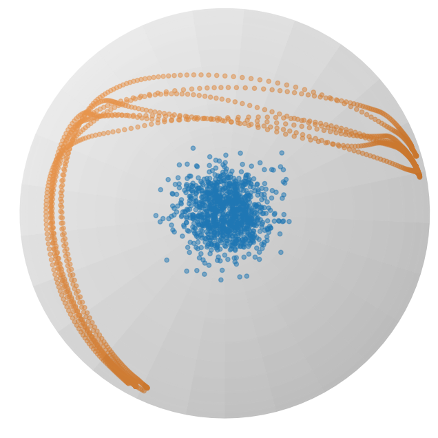
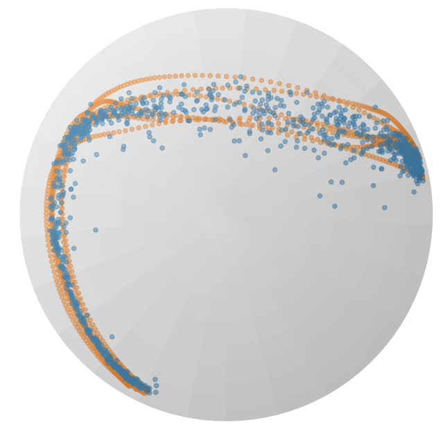
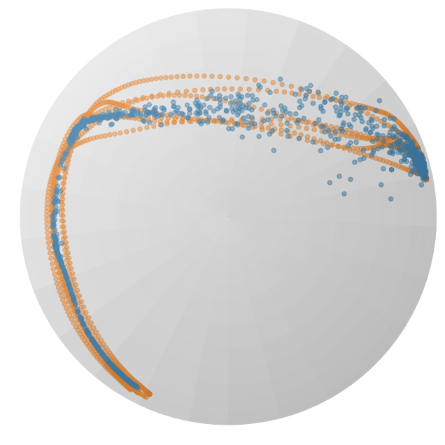
Figure 2: Flows of the RFM (top) and SRFM (bottom) trained on the $\mathsf{L}$-shape LASA dataset projected on the sphere manifold. Orange points represent the training dataset, while blue points show generated probability path at different times $t=\{0.0,1.0,1.5\}$ across the three columns.

IV-B2 Stable Riemannian FMP

1 Training Process

Input: Initial parameters ${\bm{\theta}}$, prior and target distribution $p_{0}$, $p_{1}$.

Output: Learned vector field parameters ${\bm{\theta}}$.

2 while termination condition unsatisfied do

3    Sample flow time step $t$ from an uniform distribution $\mathcal{U}[0,1]$.

4    Sample noise ${\bm{a}}_{0}\sim p_{0}$.

5    Jointly sample action sequence ${\bm{a}}_{1}\sim p_{1}$ and corresponding observation vector ${\bm{o}}$.

6    Form the vectors $\bm{\xi}_{1}=[{\bm{a}}_{1},\tau_{1}]$ and $\bm{\xi}_{0}=[{\bm{a}}_{0},\tau_{0}]$.

7    Compute conditional vector field $u_{t}(\bm{\xi}_{t}|\bm{\xi}_{1})$ via (14).

8    Evaluate the loss $\ell_{\text{SRFMP}}$ as defined in (22).

9    Update parameters ${\bm{\theta}}$.

10Inference Step

Input: Predefined number of function evaluation $N$, learned vector field $v_{{\bm{\theta}}}$, observation vector ${\bm{o}}$ and prior distribution $p_{0}$.

11 Sample ${\bm{a}}_{0}\sim p_{0}$, and set $t=0$, $\bm{\xi}_{0}=[{\bm{a}}_{0},\tau_{0}]$.

12 while $t\leq N$ do

13    Update time step $t=t+1$,

14    if $t=1$ then

15       $\Delta t=\frac{1}{\lambda_{{\bm{x}}}}$

16   else

17       $\Delta t=\varepsilon<\frac{1}{\lambda_{{\bm{x}}}}$

18   Integration on the learned Riemannian vector field $\bm{\xi}_{t}=\text{Exp}_{\bm{\xi}_{t-1}}(v_{{\bm{\theta}}}(\bm{\xi}_{t-1},{\bm{o}})\Delta t)$

Algorithm 2 SRFMP Training & Inference Process

Next, we introduce our extension, stable Riemannian flow matching (SRFM), which generalizes SFM [20] to Riemannian manifolds. Similarly as SFM, we define a time-invariant vector field $u$ by augmenting the state space with the pseudo-time state $\tau$, so that $\bm{\xi}=[{\bm{x}},\tau]$. Notice that, in this case, ${\bm{x}}\in\mathcal{M}$ and thus $\bm{\xi}$ lies on the product of Riemannian manifolds $\mathcal{M}\times\mathbb{R}$. Importantly, Theorem 1 also holds for Riemannian autonomous systems, in which case $\nabla_{{\bm{x}}}H({\bm{x}})$ denotes the Riemannian gradient of the positive scalar function $H$. We formulate $H$ so that the pair $(H,\bm{\xi})$ satisfies (12) as,

$$H(\bm{\xi}|\bm{\xi}_{1})=\frac{1}{2}\text{Log}_{\bm{\xi}_{1}}(\bm{\xi})^{\top}{\bm{A}}\text{Log}_{\bm{\xi}_{1}}(\bm{\xi}),$$ (18)

which leads to the Riemannian vector field,

$$u(\bm{\xi}|\bm{\xi}_{1})=-\nabla_{\bm{\xi}}H(\bm{\xi})^{\top}=-{\bm{A}}\text{Log}_{\bm{\xi}_{1}}(\bm{\xi}).$$ (19)

By setting the positive-definite matrix ${\bm{A}}$ as in (15), we obtain the Riemannian vector field,

$$u(\bm{\xi}_{t}|\bm{\xi}_{1})=\left[\begin{aligned} u_{\bm{x}}({\bm{x}}_{t}|{\bm{x}}_{1})\\ u_{\tau}(\tau_{t}|\tau_{1})\end{aligned}\right]=\left[\begin{aligned} -\lambda_{\bm{x}}\text{Log}_{{\bm{x}}_{1}}({\bm{x}}_{0})\\ -\lambda_{\tau}(\tau_{0}-\tau_{1})\end{aligned}\right],$$ (20)

which generates the stable Riemannian flow,

$$\psi_{t}(\bm{\xi}_{0}|\bm{\xi}_{1})=\left[\begin{aligned} \psi_{t}({\bm{x}}_{0}|{\bm{x}}_{1})\\ \psi_{t}(\tau_{0}|\tau_{1})\end{aligned}\right]=\left[\begin{aligned} \text{Exp}_{{\bm{x}}_{1}}\left(e^{-\lambda_{\bm{x}}t}\text{Log}_{{\bm{x}}_{1}}({\bm{x}}_{0})\right)\\ \tau_{1}+e^{-\lambda_{\tau}t}(\tau_{0}-\tau_{1})\end{aligned}\right].$$ (21)

The parameters $\lambda_{\bm{x}}$ and $\lambda_{\tau}$ have the same influence as in the Euclidean case. Notice that the spatial part of the stable flow (21) closely resembles the geodesic flow (8) proposed in [16]. Figure 2 shows an example of learned RFM and SRFM flows at times $t=\{0,1,1.5\}$. The RFM flow diverges from the target distribution at times $t>1$, while the SRFM flow is stable and adheres to the target distribution for $t\geq 1$.

Finally, the process to induce this stable behavior into the RFMP flow involves two main changes: (1) We define an augmented action horizon vector $\bm{\xi}=\left[{\bm{a}}^{s},\ldots,{\bm{a}}^{s+T_{p}},\tau\right]$, and; (2) We regress the observation-conditioned Riemannian vector field $v(\bm{\xi}|{\bm{o}};{\bm{\theta}})$ against the stable Riemannian vector field $u(\bm{\xi}|\bm{\xi}_{1})$ defined in (19), where ${\bm{o}}$ denotes the observation vector. The model is then trained to minimize the SRFMP loss,

$$\ell_{\text{SRFMP}}=\mathbb{E}_{t,q({\bm{a}}_{1}),p({\bm{a}}_{0})}\Arrowvert v(\bm{\xi}_{t}|{\bm{o}};{\bm{\theta}})-u(\bm{\xi}_{t}|\bm{\xi}_{1})\Arrowvert_{g_{{\bm{a}}_{t}}}^{2}.$$ (22)

This approach, hereinafter referred to as stable Riemannian flow matching policy (SRFMP), is summarized in Algorithm 2. The learned SRFMP vector field drives the flow to converge to the target distribution within a certain time horizon, ensuring that it remains within this distribution, as illustrated by the bottom row of Figures 1 and 2. In contrast, the RFMP vector field may drift the flow away from the target distribution at $t>1$ (see Figures 1 and 2, top row). Therefore, SRFMPs provide flexibility and increased robustness in designing the generation process, while RFMPs are more sensitive to the integration process.

IV-B3 Solving the SRFMP ODE

As previously discussed, querying SRFMP policies involves integrating the learned vector field along the time interval $t=[0,T]$ with time boundary $T$. To do so, we use the projected Euler method, which integrates the vector field on the tangent space for one Euler step and then projects the resulting vector onto the manifold $\mathcal{M}$. Assuming an Euclidean setting and that $v(\bm{\xi}|{\bm{o}};{\bm{\theta}})$ is perfectly learned, this corresponds to recursively applying,

$${\bm{x}}_{t+1}={\bm{x}}_{t}+v_{{\bm{x}}}({\bm{x}}_{t}|{\bm{o}};{\bm{\theta}})\Delta t\,\approx\,{\bm{x}}_{t}+\lambda_{\bm{x}}({\bm{x}}_{1}-{\bm{x}}_{t})\Delta t,$$ (23)

with time step $\Delta t$ and $v_{{\bm{x}}}$ following the same partitioning as $u_{{\bm{x}}}$ in (20). The time step $\Delta t$ is typically set as $\Delta t=T/N$, where $N$ is the total number of ODE steps. Here we propose to leverage the structure of SRFMP to choose the time step $\Delta t$ in order to further speed up the inference time of RFMP. Specifically, we observe that the recursion (23) leads to,

$${\bm{x}}_{t}=(1-\lambda_{{\bm{x}}}\Delta t)^{n}({\bm{x}}_{0}-{\bm{x}}_{1})+{\bm{x}}_{1},$$ (24)

after $n$ time steps. It is easy to see that ${\bm{x}}_{t}$ converges to ${\bm{x}}_{1}$ after a single time step when setting $\Delta t=1/\lambda_{{\bm{x}}}$.

In the Riemannian case, assuming that $v(\bm{\xi}|{\bm{o}};{\bm{\theta}})$ approximately equals the Riemannian vector field (20), we obtain,

$${\bm{x}}_{t+1}=\text{Exp}_{{\bm{x}}_{t}}\left(v_{{\bm{x}}}({\bm{x}}|{\bm{o}};{\bm{\theta}})\Delta t\right)\,\approx\,\text{Exp}_{{\bm{x}}_{t}}\left(\lambda_{\bm{x}}\text{Log}_{{\bm{x}}_{t}}({\bm{x}}_{1})\Delta t\right).$$ (25)

Similarly, it is easy to see that the Riemannian flow converges to ${\bm{x}}_{1}$ after a single time step for $\Delta t=1/\lambda_{{\bm{x}}}$. Importantly, this strategy assumes that the learned vector field is perfectly learned and thus equals the target vector field. However, this is often not the case in practice. However, our experiments show that the flow obtained solving the SRFMP ODE with a single time step $\Delta t=1/\lambda_{\bm{x}}$ generally leads to the target distribution. In practice, we set $\Delta t$ to $1/\lambda_{\bm{x}}$ for the first time step, and to a smaller value afterwards for refining the flow.

V Experiments

We thoroughly evaluate the performance of RFMP and SRFMP on a set of six simulation settings and two real-world tasks. The simulated benchmarks are: (1) The Push-T task from [2]; (2) A Sphere Push-T task, which we introduce as a Riemannian benchmark; and (3)-(6) Four tasks (Lift, Can, Square, and Tool Hang) from the large-scale robot manipulation benchmark Robomimic [10]. The real-world robot tasks correspond to: (1) A Pick & Place task; and (2) A Mug Flipping task. Collectively, these eight tasks serve as a benchmark to evaluate (1) the performance, (2) the training time, and (3) the inference time of RFMP and SRFMP with respect to state-of-the-art generative policies, i.e., DP and extensions thereof.

V-A Implementation Details

To establish a consistent experimental framework, we first introduce the neural network architectures employed in RFMP and SRFMP across all tasks. We then describe the considered baselines, and our overall evaluation methodology.

V-A1 RFMP and SRFMP Implementation

Our RFMP implementation builds on the RFM framework from Chen and Lipman [16]. We parameterized the vector field $v_{t}(\bm{a}|\bm{o};\bm{\theta})$ using the UNet architecture employed in DP [2], which consists of $3$ layers with downsampling dimensions of $(256,512,1024)$ and $(128,256,512)$ for simulated and real-world tasks. Each layer employs a $1$-dimensional convolutional residual network as proposed in [29]. We implement a Feature-wise Linear Modulation (FiLM) [58] to incorporate the observation condition vector ${\bm{o}}$ and time step $t$ into the UNet. Instead of directly feeding the FM time step $t$ as a conditional variable, we first project it into a higher-dimensional space using a sinusoidal embedding module, similarly to DP. For tasks with image-based observations, we leverage the same vision perception backbone as in DP [2]. Namely, we use a standard ResNet-$18$ in which we replace: (1) the global average pooling with a spatial softmax pooling, and (2) BatchNorm with GroupNorm. Our SRFMP implementation builds on the SFM framework [20]. We implement the same UNet as RFMP to represent $v_{{\bm{x}}}$ by replacing the time step $t$ by the temperature parameter $\tau$. We introduce an additional Multi-Layer Perceptron (MLP) to learn $v_{\tau}$. As for $t$ in RFMP, we employed a sinusoidal embedding for the input $\tau$. The boundaries $\tau_{0}$ and $\tau_{1}$ are set to $0$ and $1$ in all experiments.

We implement different prior distributions for different tasks. For the Euclidean Push-T and the four Robomimic tasks, the action space is $\mathbb{R}^{d}$ and we thus define the prior distribution as a Euclidean Gaussian distribution for both RFMP and SRFMP. For the Sphere Push-T, the action space is the hypersphere $\mathcal{S}^{2}$. In this case, we test two types of Riemannian prior distribution, namely a spherical uniform distribution, and a wrapped Gaussian distribution [59, 60], illustrated in Figure 3. Regarding the real robot tasks, the task space is defined as the product manifold $\mathcal{M}=\mathbb{R}^{3}\times\mathcal{S}^{3}\times\mathbb{R}^{1}$, whose components represent the position, orientation (encoded as quaternions), and opening of the gripper. The Euclidean and hypersphere parts employ Euclidean Gaussian distributions and a wrapped Gaussian distribution, respectively.

TABLE I: Hyperparameters for all experiments: Resolution of original and cropped image, number of parameters for the learned vector field using RFMP and SRFMP, number of ResNet parameters, training epochs and batch size.

Experiment	Image res.	Crop res.	RFMP VF Num. params	SRFMP VF Num. params	ResNet params	Epochs	Batch size
Push-T Tasks
Eucl. Push-T task	$96\times 96$	$84\times 84$	$8.0\text{\times}{10}^{07}$	$8.14\text{\times}{10}^{07}$	$1.12\text{\times}{10}^{07}$	$300$	$256$
Sphere Push-T task	$100\times 100$	$84\times 84$	$8.0\text{\times}{10}^{07}$	$8.14\text{\times}{10}^{07}$	$1.12\text{\times}{10}^{07}$	$300$	$256$
State-based Robomimic
Lift	N.A.	N.A.	$6.58\text{\times}{10}^{07}$	$6.68\text{\times}{10}^{07}$	N.A.	50	256
Can	N.A.	N.A.	$6.58\text{\times}{10}^{07}$	$6.68\text{\times}{10}^{07}$	N.A.	$50$	$256$
Square	N.A.	N.A.	$6.58\text{\times}{10}^{07}$	$6.68\text{\times}{10}^{07}$	N.A.	$50$	$512$
Tool Hang	N.A.	N.A.	$6.58\text{\times}{10}^{07}$	$6.68\text{\times}{10}^{07}$	N.A.	$100$	$512$
Vision-based Robomimic
Lift	$2\times 84\times 84$	$2\times 76\times 76$	$9.48\text{\times}{10}^{07}$	$9.69\text{\times}{10}^{07}$	$2\times$1.12\text{\times}{10}^{07}$$	100	256
Can	$2\times 84\times 84$	$2\times 76\times 76$	$9.48\text{\times}{10}^{07}$	$9.69\text{\times}{10}^{07}$	$2\times$1.12\text{\times}{10}^{07}$$	100	256
Square	$2\times 84\times 84$	$2\times 76\times 76$	$9.48\text{\times}{10}^{07}$	$9.69\text{\times}{10}^{07}$	$2\times$1.12\text{\times}{10}^{07}$$	100	512
Real-world experiments
Pick & place	$320\times 240$	$288\times 216$	$2.51\text{\times}{10}^{07}$	$2.66\text{\times}{10}^{07}$	$1.12\text{\times}{10}^{07}$	$300$	$256$
Rotate mug	$320\times 240$	$256\times 192$	$2.51\text{\times}{10}^{07}$	$2.66\text{\times}{10}^{07}$	$1.12\text{\times}{10}^{07}$	$300$	$256$

For all experiments, we optimize the network parameters of RFMP and SRFMP using AdamW [61] with a learning rate of $\eta=1\times 10^{-4}$ and weight decay of $w_{d}=0.001$ based on an exponential moving averaging (EMA) framework on the weights [62] with a decay of $w_{\text{EMA}}=0.999$. Moreover, we use an action prediction horizon $T_{p}=16$, an action horizon $T_{a}=T_{p}/2$, and an observation horizon $T_{o}=2$. We set the SRFMP parameters as $\lambda_{{\bm{x}}}=\lambda_{\tau}=2.5$. Table I summarizes the image resolution, number of parameters, and number of training epochs used in each experiment.

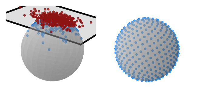
Figure 3: 2D visualization of prior distributions used in the Sphere Push-T task: wrapped Gaussian distribution (left) and sphere uniform distribution (right). The sphere Gaussian distribution is obtained by first sampling from a Euclidean Gaussian distribution on a tangent space of the sphere (the red points), followed by the exponential map, which projects the samples onto the sphere manifold $\mathcal{S}^{d}$ (blue points). The spherical uniform distribution is computed by normalizing samples from a zero-mean Euclidean Gaussian distribution.

V-A2 Baselines

In the original DP paper [2], the policy is trained using either Denoising Diffusion Probabilistic Model (DDPM) [12] or Denoising Diffusion Implicit Model (DDIM) [13]. In this paper, we prioritize faster inference and thus employ DDIM-based DP for all our experiments. We train DDIM with $100$ denoising steps. The prior distribution is a standard Gaussian distribution unless explicitly mentioned. During training we use the same noise scheduler as in [2], the optimizer AdamW with the same learning rate and weight decay as for RFMP and SRFMP. Note that DP does not handle data on Riemannian manifolds, and thus does not guarantee that the resulting trajectories lie on the manifold of interest for tasks with Riemannian action spaces, e.g., the Sphere Push-T and real-world robot experiments. In these cases, we post-process the trajectories obtained during inference and project them on the manifold. In the case of the hypersphere manifold, the projection corresponds to a unit-norm normalization. We also compare RFMP and SRFMP against CP [3] on the Robomimic tasks with vision-based observations. To do so, we use the performance values reported in [3].

V-A3 Evaluation methodology

We evaluate RFMP, SRFMP, and DP using three key metrics: (1) The performance, computed as the average task-depending score across all trials, with $50$ trials for each simulated task, and $10$ trials for each real-world task; (2) The number of training epochs; and (3) The inference time. To provide a consistent measure of inference time across RFMP, SRFMP, and DP, we report it in terms of the number of function evaluations (NFE), which is proportional to the inference process time. Given that each function evaluation takes approximately the same time across all methods, inference time comparisons can be made directly based on NFE. For example, in real-world tasks, with an NFE of $2$, DP requires around $0.0075$\mathrm{s}$$, while RFMP and SRFMP take approximately $0.0108$\mathrm{s}$$ and $0.0113$\mathrm{s}$$, respectively. When NFE is increased to $5$, DP takes around $0.0175$\mathrm{s}$$, while RFMP and SRFMP require about $0.021$\mathrm{s}$$ and $0.0212$\mathrm{s}$$.

V-B Push-T Tasks

We first consider two simple Push-T tasks, namely the Euclidean Push-T proposed in [2], which was adapted from the Block Pushing task [8], and the Sphere Push-T task, which we introduce shortly. The goal of the Euclidean Push-T task, illustrated in Figure 4, is to push a gray T-shaped object to the designated green target area with a blue circular agent. The agent’s movement is constrained by a light gray square boundary. Each observation ${\bm{o}}$ is composed of the $96\times 96$ RGB image of the current scene and the agent’s state information. We introduce the Sphere Push-T task, visualized in Figure 4, to evaluate the performance of our models on the sphere manifold. Its environment is obtained by projecting the Euclidean Push-T environment on one half of a $2$-dimensional sphere $\mathcal{S}^{2}$ of radius of $1$. This is achieved by projecting the environment, normalized to a range $[-1.5,1.5]$, from the plane $z=1$ to the sphere via a stereographic projection. The target area, the T-shaped object, and the agent then lie and evolve on the sphere. As in the Euclidean case, each observation ${\bm{o}}$ is composed of the $96\times 96$ RGB image of the current scene and the agent’s state information on the manifold. All models (i.e., RFMP, SRFMP, DP) are trained for $300$ epochs in both settings. During testing, we choose the best validation epoch and only roll out $500$ steps in the environment with an early stop rule terminating the execution when the coverage area is over $95\%$ of the green target area. The score for both Euclidean and Sphere Push-T tasks is the maximum coverage ratio during execution. The tests are performed with $50$ different initial states not present in the training set.

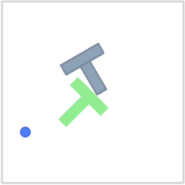
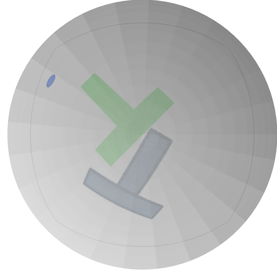
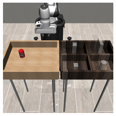
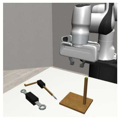
Figure 4: Simulation benchmarks: Euclidean Push-T [2], Sphere Push-T, and four tasks from Robomimic [10]: Lift, Can, Square, Tool Hang.

V-B1 Euclidean Push-T

First, we evaluate the performance of RFMP and SRFMP in the Euclidean case for different number of function evaluations in the testing phase. The models are trained with the default parameters described in Section V-A1. Table II shows the success rate of RFMP and SRFMP for different NFEs. We observe that both RFMP and SRFMP achieve similar success rates overall. While SRFMP demonstrates superior performance with a single NFE, RFMP achieves higher success rates with more NFEs. We hypothesize that this behavior arises from the fact that, due to the equality $\lambda_{\bm{x}}=\lambda_{\tau}$, the SRFMP conditional probability path resembles the optimal transport map between the prior and target distributions as in [15]. This, along with the stability framework of SRFMP, allows us to automatically choose the timestep during inference via (24), which enhances convergence in a single step. When comparing our approaches with DP, we observe that DP performs drastically worse than both RFMP and SRFMP for a single NFE, achieving a score of only $10.9\%$. Nevertheless, the performance of DP improves when increasing the NFE and matches that of our approaches for $10$ NFE.

TABLE II: Euclidean Push-T: Impact of NFE on policies

	NFE
Policy	1	3	5	10
RFMP	$0.848$	$\bm{0.855}$	$\bm{0.923}$	$\bm{0.891}$
SRFMP	$\bm{0.875}$	$0.851$	$0.837$	$0.856$
DP	$0.109$	$0.79$	$0.838$	$0.862$

Next, we ablate the action prediction horizon $T_{p}$, observation horizon $T_{o}$, learning rate $\eta$, and weight decay $w_{d}$ for RFMP and SRFMP. We consider $3$ different values for each, while setting the other hyperparameters to their default values, and test the resulting models with $5$ different NFE. For SRFMP, we additionally ablate the parameters $\lambda_{\bm{x}}$ and $\lambda_{\tau}$ for $3$ different ratios $\lambda_{\bm{x}}/\lambda_{\tau}$ and $4$ values for each ratio. Each setup is tested with $50$ seeds, resulting in a total of $2250$ and $4000$ experiments for RFMP and SRFMP. The results are reported in Tables III and IV, respectively. We observe that a short observation horizon $T_{o}=2$ leads to the best performance for both models. This is consistent with the task, as the current and previous images accurately provide the required information for the next pushing action, while the actions associated with past images rapidly become outdated. Moreover, we observe that an action prediction horizon $T_{p}=16$ leads to the highest score. We hypothesize that this horizon allows the model to maintain temporal consistency, while providing frequent enough updates of the actions according to the current observations. Concerning SRFMP, we find that $\lambda_{\bm{x}}=\lambda_{\tau}=2.5$ leads to the highest success rates. Interestingly, this choice leads to the ratio $\lambda_{\bm{x}}/\lambda_{\tau}=1$, in which case the flow of ${\bm{x}}$ follows the Gaussian CFM (6) of [15] with $\sigma\to 0$ for $\tau=[0,1]$, see [20, Cor 4.12]. In the next experiments, we use the default parameters resulting from our ablations, i.e., $T_{p}=16$, $T_{o}=2$, $\eta=1\times 10^{-4}$, $w_{d}=0.001$, and $\lambda_{\bm{x}}=\lambda_{\tau}=2.5$.

TABLE III: RFMP Hyperparameters Ablation on Euclidean Push-T

Parameter	Values	Success rate
NFE		$1$	$3$	$5$	$10$	$100$
$T_{o}$	${\color[rgb]{0.0,0.39,0.0}\bm{2}}$	$\bm{0.848}$	$\bm{0.855}$	$\bm{0.923}$	$\bm{0.891}$	$\bm{0.91}$
	$8$	$0.195$	$0.16$	$0.154$	$0.168$	$0.179$
	$16$	$0.135$	$0.143$	$0.14$	$0.133$	$0.135$
	$8$	$0.754$	$0.835$	$0.827$	$0.839$	$0.85$
	${\color[rgb]{0.0,0.39,0.0}\bm{16}}$	$\bm{0.848}$	$0.855$	$\bm{0.923}$	$0.891$	$0.91$
$T_{p}$	$32$	$0.799$	$\bm{0.906}$	$0.878$	$\bm{0.929}$	$\bm{0.93}$
$\eta$	${\color[rgb]{0.0,0.39,0.0}\bm{1\times 10^{-4}}}$	$\bm{0.848}$	$0.855$	$0.923$	$0.891$	$0.91$
	$5\text{\times}{10}^{-5}$	$0.797$	$0.863$	$0.843$	$0.897$	$0.889$
	$1\text{\times}{10}^{-5}$	$0.641$	$0.771$	$0.805$	$0.88$	$0.841$
	${\color[rgb]{0.0,0.39,0.0}\bm{0.001}}$	$0.848$	$0.855$	$\bm{0.923}$	$0.891$	$\bm{0.91}$
	$0.005$	$0.846$	$\bm{0.882}$	$0.875$	$0.866$	$0.856$
$w_{d}$	$0.01$	$\bm{0.868}$	$0.831$	$0.842$	$\bm{0.927}$	$0.853$

TABLE IV: SRFMP Hyperparameters Ablation on Euclidean Push-T

Parameter	Values	Success rate
NFE		$1$	$3$	$5$	$10$
$T_{o}$	${\color[rgb]{0.0,0.39,0.0}\bm{2}}$	$\bm{0.875}$	$\bm{0.851}$	$\bm{0.837}$	$\bm{0.856}$
	$8$	$0.124$	$0.139$	$0.147$	$0.13$
	$16$	$0.145$	$0.138$	$0.149$	$0.144$
	$8$	$0.816$	$0.726$	$0.592$	$0.318$
	${\color[rgb]{0.0,0.39,0.0}\bm{16}}$	$\bm{0.875}$	$0.851$	$0.837$	$\bm{0.856}$
$T_{p}$	$32$	$0.852$	$\bm{0.861}$	$\bm{0.881}$	$0.829$
$\eta$	${\color[rgb]{0.0,0.39,0.0}\bm{1.0\times 10^{-4}}}$	$\bm{0.875}$	$\bm{0.851}$	$\bm{0.837}$	$\bm{0.856}$
	$5\text{\times}{10}^{-5}$	$0.754$	$0.621$	$0.456$	$0.334$
	$1\text{\times}{10}^{-5}$	$0.602$	$0.56$	$0.443$	$0.288$
	${\color[rgb]{0.0,0.39,0.0}\bm{0.001}}$	$\bm{0.875}$	$\bm{0.851}$	$\bm{0.837}$	$\bm{0.856}$
	$0.005$	$0.837$	$0.826$	$0.826$	$0.684$
$w_{d}$	$0.01$	$0.733$	$0.75$	$0.768$	$0.571$
$\lambda_{{\bm{x}}}\quad\lambda_{\tau}$	$1$ $0.2$	$0.74$	$0.614$	$0.494$	$0.457$
	$1$ $1$	$0.85$	$0.777$	$0.608$	$0.416$
	$1$ $6$	$0.87$	$0.768$	$0.753$	$0.812$
	$2.5$ $0.2$	$0.832$	$0.392$	$0.576$	$0.549$
	${\color[rgb]{0.0,0.39,0.0}\bm{2.5}}$ ${\color[rgb]{0.0,0.39,0.0}\bm{2.5}}$	$\bm{0.875}$	$\bm{0.851}$	$0.837$	$\bm{0.856}$
	$2.5$ $15$	$0.832$	$0.799$	$0.789$	$0.807$
	$5$ $1$	$0.796$	$0.741$	$0.614$	$0.513$
	$5$ $5$	$0.845$	$0.825$	$0.797$	$0.642$
	$5$ $30$	$0.822$	$0.830$	$0.772$	$0.743$
	$7.5$ $1.5$	$0.799$	$0.685$	$0.442$	$0.456$
	$7.5$ $7.5$	$0.787$	$0.8$	$0.809$	$0.633$
	$7.5$ $45$	$0.782$	$0.817$	$\bm{0.844}$	$0.814$

V-B2 Sphere Push-T

Next, we test the ability of RFMP and SRFMP to generate motions on non-Euclidean manifolds with the Sphere Push-T task. We evaluate two types of Riemannian prior distributions for RFMP and SRFMP, namely a spherical uniform distribution and wrapped Gaussian distribution. We additionally consider a Euclidean Gaussian distribution for DP. Notice that the actions generated by DP are normalized in a post-processing step to ensure that they belong to the sphere. The corresponding performance are reported in Table V. Our results indicate that the choice of prior distribution significantly impacts the performance of both RFMP and SRFMP. Specifically, we observe that RFMP and SRFMP with a uniform sphere distribution consistently outperform their counterparts with wrapped Gaussian distribution. We hypothesize that RFMP or SRFMP benefit from having samples that are close to the data support, which leads to simpler vector fields to learn. In other words, uniform distribution provides more samples around the data distribution, which potentially lead to simpler vector fields. DP exhibit poor performance with sphere-based prior distributions, suggesting its ineffectiveness in handling such priors. Instead, DP’s performance drastically improves when using a Euclidean Gaussian distribution and higher NFE. Note that this high performance does not scale to higher dimensional settings as already evident in the real-world experiments reported in Section V-D, where the effect of ignoring the geometry of the parameters exacerbates, which is a known issue when naively operating with Riemannian data [63]. Importantly, SRFMP is consistently more robust to NFE and achieves high performance with a single NFE, leading to shorter inference times for similar performance compared to RFMP and DP.

TABLE V: Impact of the prior distribution on Sphere Push-T Task

	NFE
Policy	$1$	$3$	$5$	$10$
RFMP sphere uniform	$\bm{0.871}$	$0.746$	$0.77$	$0.817$
RFMP sphere Gaussian	$0.587$	$0.724$	$0.748$	$0.733$
SRFMP sphere uniform	$0.772$	$0.736$	$0.796$	$0.829$
SRFMP sphere Gaussian	$0.707$	$0.706$	$0.735$	$0.707$
DP sphere uniform	$0.274$	$0.261$	$0.235$	$0.197$
DP sphere Gaussian	$0.170$	$0.162$	$0.231$	$0.227$
DP euclidean Gaussian	$0.227$	$\bm{0.796}$	$\bm{0.813}$	$\bm{0.885}$

TABLE VI: Influence of Integration Time on RFMP and SRFMP

Euclidean Push-T	$t=1.0$	$t=1.2$	$t=1.6$
RFMP	$0.855$	$0.492$	$0.191$
SRFMP	$\bm{0.862}$	$\bm{0.851}$	$\bm{0.829}$
Sphere Push-T	$t=1.0$	$t=1.2$	$t=1.6$
RFMP	$\bm{0.736}$	$0.574$	$0.264$
SRFMP	$0.727$	$\bm{0.736}$	$\bm{0.685}$

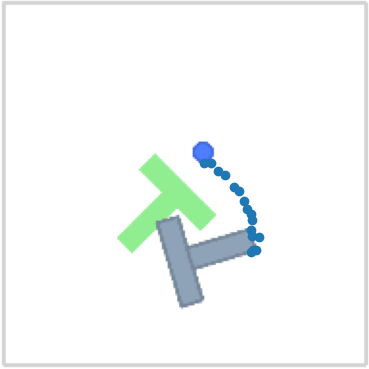
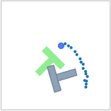
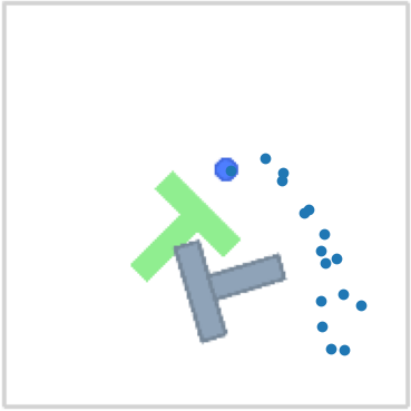
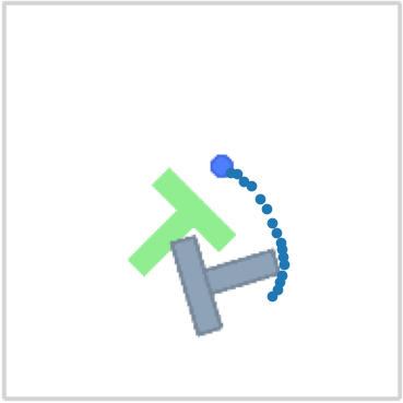
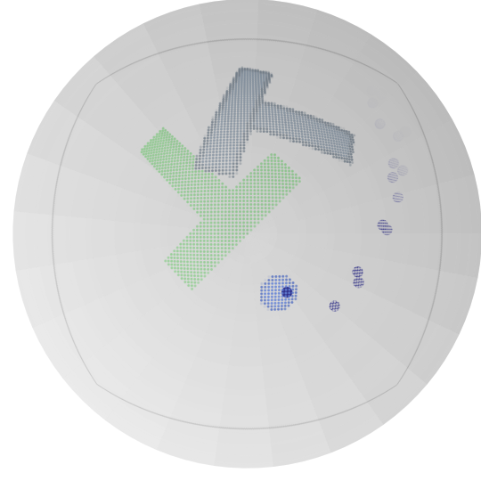
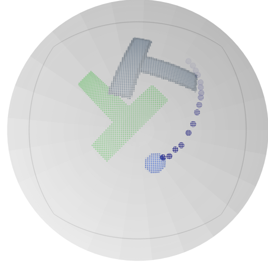
Figure 5: Action series generated by RFMP (first and third rows) and SRFMP (second and forth rows) trained on the Push-T tasks at integration times $t=\{0.8,1.2,1.6\}$.

V-B3 Influence of Integration Time Boundary

We further assess the robustness of SRFMP to varying time boundaries on the Push-T tasks by increasing the time boundary during inference. The performance of both RFMP and SRFMP is summarized in Table VI with result presented for $\text{NFE}=3$ under the time boundaries $t=1$ and $t=1.2$, as well as for $\text{NFE}=4$ under the time boundaries $t=1.6$. Our results show that the performance of RFMP is highly sensitive to the time boundary, gradually declining as the boundary increases. In contrast, SRFMP demonstrates remarkable robustness, with minimal variation across different time boundaries. As illustrated in Figure 5, the quality of action series generated by RFMP noticeably deteriorates with increasing time boundaries, whereas SRFMP consistently delivers high-quality action series regardless of the time boundary.

V-C Simulated Robotic Experiments

Next, we evaluate RFMP and SRFMP on the well-known Robomimic robotic manipulation benchmark [10]. This benchmark consists of five tasks with varying difficulty levels. The benchmark provides two types of demonstrations, namely proficient human (PH) high-quality teleoperated demonstrations, and mixed human (MH) demonstrations. Each demonstration contains multi-modal observations, including state information, images, and depth data. We report results on four tasks (Lift, Can, Square, and Tool Hang) from the Robomimic dataset with $200$ PH demonstrations for training for both state- and vision-based observations. Note that the difficulty of the selected tasks becomes progressively more challenging. The score of each of the $50$ trials is determined by whether the task is completed successfully after a given number of steps ($300$ for Lift, $500$ for Can and Square, and $700$ for Tool Hang. The performance is then the percentage of successful trials.

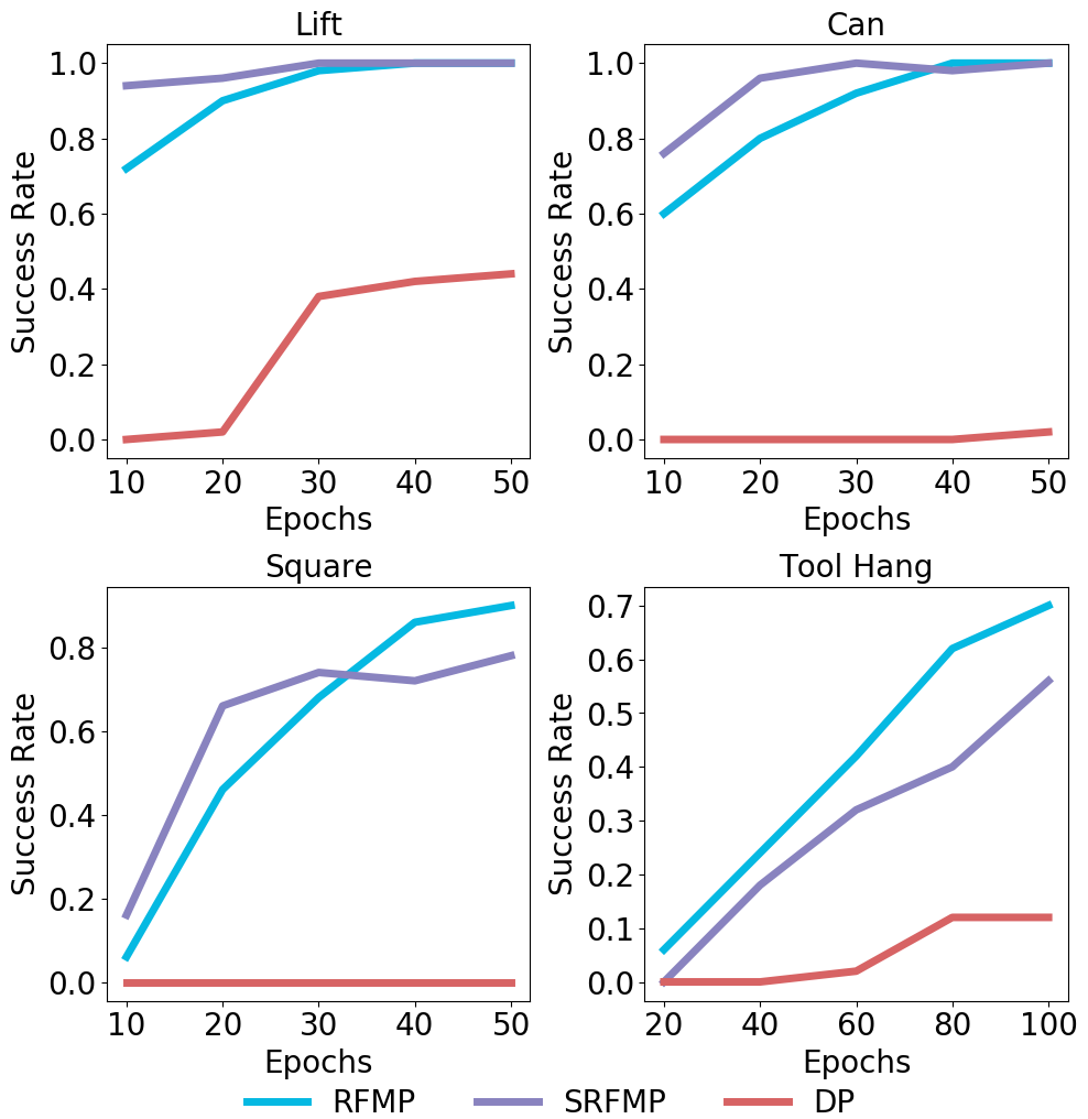
Figure 6: Success rate on Robomimic tasks with state-based observations at different checkpoints. The models performance of Lift, Can, and Square tasks is checked every $10$ epochs throughout the $50$-epoch training process using $3$ NFE. For the Tool Hang task, the models are trained over $100$ epochs and checked every $20$ epochs using $10$ NFE.

V-C1 State-based Observations

We first assess the training efficiency of RFMP and SRFMP and compare it against DP by analyzing their performance at different training stages. Figure 6 shows the success rate of the three policies as a function of the number of training epochs for each task. All policies are evaluated with $3$ NFE for Lift, Can, and Square, and with $10$ NFE for Tool Hang. We observe that RFMP and SRFMP consistently outperform DP across all tasks, requiring fewer training epochs to achieve comparable or superior performance. For the easier tasks (Lift and Can), both RFMP and SRFMP achieve high performance after just $20$ training epochs, while the success rate of DP remains low after $50$ epochs. This trend persists in the harder tasks (Square and Tool Hang), with RFMP and SRFMP reaching high success rates significantly faster than DP.

TABLE VII: Success rate as a function of different NFE values on the state-based Robomimic tasks.

Task	Lift					Can					Square					Tool Hang
NFE	$1$	$2$	$3$	$5$	$10$	$1$	$2$	$3$	$5$	$10$	$1$	$2$	$3$	$5$	$10$	$1$	$2$	$3$	$5$	$10$
RFMP	$\bm{1}$	$\bm{1}$	$\bm{1}$	$0.98$	$\bm{1}$	$\bm{0.96}$	$\bm{1}$	$\bm{1}$	$\bm{0.98}$	$0.96$	$\bm{0.78}$	$\bm{0.82}$	$\bm{0.9}$	$\bm{0.84}$	$\bm{0.9}$	$0.16$	$\bm{0.3}$	$\bm{0.36}$	$\bm{0.56}$	$\bm{0.7}$
SRFMP	$\bm{1}$	$\bm{1}$	$\bm{1}$	$\bm{1}$	$\bm{1}$	$0.94$	$0.96$	$\bm{1}$	$\bm{0.98}$	$\bm{0.98}$	$0.72$	$0.7$	$0.78$	$0.7$	$0.72$	$\bm{0.26}$	$0.2$	$0.28$	$0.5$	$0.56$
DP	$0$	$0.78$	$0.96$	$0.96$	$0.98$	$0$	$0.38$	$0.82$	$0.92$	$0.9$	$0$	$0.4$	$0.62$	$0.66$	$0.66$	$0$	$0$	$0.04$	$0.1$	$0.08$

TABLE VIII: Jerkiness of predicted robot trajectories for different NFE on the robomimic tasks with state-based observations. All values are expressed in thousands, where the lower the smoother the prediction.

Task	Lift					Can					Square					Tool Hang
NFE	$1$	$2$	$3$	$5$	$10$	$1$	$2$	$3$	$5$	$10$	$1$	$2$	$3$	$5$	$10$	$1$	$2$	$3$	$5$	$10$
RFMP	$\bm{9.75}$	$\bm{8.82}$	$9.05$	$\bm{8.82}$	$\bm{8.44}$	$7.92$	$\bm{6.62}$	$6.59$	$\bm{6.45}$	$9.68$	$\bm{9.11}$	$\bm{6.39}$	$\bm{5.49}$	$\bm{5.3}$	$\bm{4.29}$	$\bm{4.43}$	$\bm{3.98}$	$\bm{4.54}$	$\bm{5.25}$	$\bm{4.79}$
SRFMP	$10.2$	$10.1$	$\bm{7.79}$	$9.75$	$9.35$	$\bm{7.6}$	$7.75$	$\bm{6.35}$	$7.16$	$\bm{6.86}$	$9.29$	$9.67$	$6.59$	$8.3$	$7.81$	$5.48$	$5.0$	$5.33$	$6.28$	$6.29$
DP	$344$	$14.4$	$8.15$	$7.3$	$8.57$	$558$	$19.9$	$6.94$	$5.93$	$6.19$	$558$	$19.9$	$7.28$	$14.7$	$5.48$	$777$	$9.42$	$9.95$	$5.39$	$7.41$

Next, we evaluate the performance of the policies for different NFE in the testing phase. For RFMP and SRFMP, we use the $50$-epoch models for Lift, Can, and Square, and the $100$-epoch model for Tool Hang. DP is further trained for a total of $300$ epochs and we select the model at the best validation epoch. The results are reported in Table VII. RFMP and SRFMP outperform DP for all task and all NFE, even though DP was trained for more epochs. Moreover, we observe that RFMP and SRFMP are generally more robust to low NFE than DP. They achieve $100$% success rate at almost all NFE values for the easier Lift and Can tasks, while DP’s performance drastically drops for $1$ and $2$ NFE. We observe a similar trend for the Square task, where the performance of RFMP and SRFMP slightly improves when increasing the NFE. The performance of all models drops for Tool Hang, which is the most complex of the considered tasks. In this case, the performance of RFMP and SRFMP is limited for low NFE values and improves for higher NFE. DP performs poorly for all considered NFE values. Table VIII reports the jerkiness as a measure of the smoothness of the trajectories generated by the different policies. We observe that RFMP and SRFMP produce arguably smoother trajectories than DP for low NFE, as indicated by the lower jerkiness values. The smoothness of the trajectories becomes comparable for higher NFE. In summary, both RFMP and SRFMP achieve high success rates and smooth action predictions with low NFE, enabling faster inference without compromising task completion.

V-C2 Vision-based Observations

Next, we assess our models performance when the vector field is conditioned on visual observations. We consider the tasks Lift, Can and Square with the same policy settings and networks (see Table I). Each observation ${\bm{o}}^{s}$ at time $s$ corresponds to the embeddings vector obtained from an image of an over-the-shoulder camera and an image of an in-hand camera. We train the models for a total $100$ epochs and use the best-performing checkpoint for evaluation. The performance of different policies is reported in Table IX. RFMP and SRFMP consistently outperform DP on all tasks, regardless of the NFE. As for the previous experiments, our models are remarkably robust to changes in NFE compared to DP. Importantly, SRFMP consistently surpassed RFMP for $1$ and $2$ NFE. Regarding Can and Square tasks, SRFMP with $1$ NFE achieved performance on par with RFMP using $3$ NFE. This efficiency gain showcases the benefits of enhancing the policies with stability to the target distribution for reducing their inference time. We additionally compare RFMP and SRFMP against CP by reporting the performance obtained from [3] in Table IX. Our models achieve a competitive performance compared to CP, which is a method aimed at steeping up inference. However, in contrast to CP, our models are easy and fast to train.

TABLE IX: Success rate as a function of NFE on vision-based robomimic tasks. The CP results correspond to those reported in [3].

Task	Lift					Can					Square
	NFE					NFE					NFE
Policy	$1$	$2$	$3$	$5$	$10$	$1$	$2$	$3$	$5$	$10$	$1$	$2$	$3$	$5$	$10$
RFMP	$\bm{1}$	$\bm{1}$	$\bm{1}$	$\bm{1}$	$\bm{1}$	$0.78$	$0.82$	$\bm{0.9}$	$\bm{0.96}$	$\bm{0.94}$	$0.56$	$0.74$	$\bm{0.9}$	$\bm{0.9}$	$\bm{0.9}$
SRFMP	$\bm{1}$	$\bm{1}$	$\bm{1}$	$\bm{1}$	$\bm{1}$	$\bm{0.88}$	$\bm{0.88}$	$\bm{0.9}$	$0.9$	$0.86$	$\bm{0.86}$	$\bm{0.82}$	$\bm{0.9}$	$0.88$	$\bm{0.9}$
DP	$0$	$0.7$	$0.96$	$0.98$	$0.98$	$0$	$0.38$	$0.66$	$0.68$	$0.66$	$0$	$0.04$	$0.16$	$0.26$	$0.12$
CP	$\underline{1}$	N.A.	$\underline{1}$	N.A.	N.A.	$\underline{0.98}$	N.A.	$\underline{0.95}$	N.A.	N.A.	$\underline{0.92}$	N.A.	$\underline{0.96}$	N.A.	N.A.

V-D Real Robotic Experiments

Finally, we evaluate RFMP and SRFMP on two real-world tasks, namely Pick & Place and Mug Flipping, with a $7$-DoF robotic manipulator.

V-D1 Experimental Setup

Figure 7 shows our experimental setup. The tasks are performed on a Franka Emika Panda robot arm. We collect the demonstrations via a teleoperation system consisting of two robot twins. Demonstrations are collected by an expert who guides the source robot. All the demonstrations were recorded in a fairly controlled environment with minimal variation in lighting and background. The target robot then reads the end-effector pose of the source robot and reproduces it via a Cartesian impedance controller. Each observation ${\bm{o}}^{s}$ is composed of the end-effector position, and of the image embedding obtained from the ResNet vision backbone that processes the images from an over-the-shoulder camera. The policies are trained to generate $8$-dimensional actions composed of the position, orientation, and gripper state.

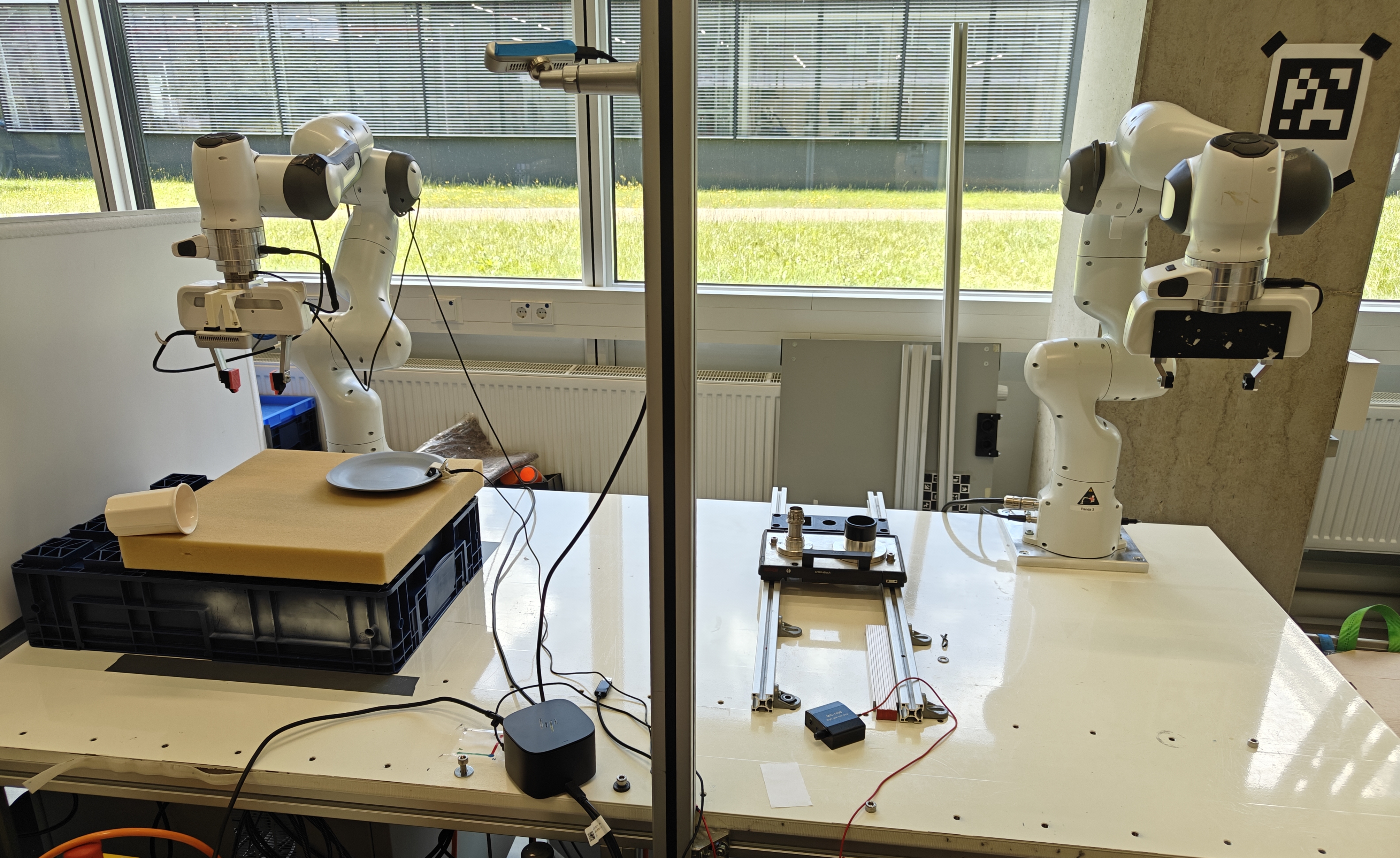
Figure 7: Robotic experimental setup consisting of $2$ Franka Emika Panda robot arms for teleoperation and an over-the-shoulder camera (Realsense d435). The left arm is follower robot, while the right one acts as the leader. During the teaching phase, a human expert controls the leader arm to send the desired reference to the follower robot via ROS. During testing, only the follower arm is operational.

V-D2 Pick & Place

The goal of this task is to test the ability of RFMP and SRFMP to learn Euclidean policies in real-world settings. The task consists of approaching and picking up a white mug, and to then place it on a pink plate, as shown in Figure 8. Note that the end effector of the robot points downwards during the entire task, so that its orientation remains almost constant.

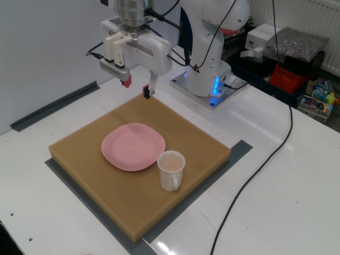
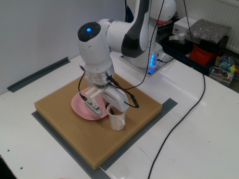
Figure 8: Pick & Place: First, the robot end-effector approaches and grasps the white mug. Then, it lifts the mug and places it upright on the pink plate.

We collect $100$ demonstrations where the white mug is randomly placed on the yellow mat, while the pink plate position and end-effector initial position are slightly varied. We split our demonstration data to use $90$ demonstrations for training and $10$ for validation. All models are trained for $300$ epochs with the same training hyperparameters as reported in Table I. As in previous experiments, we use the best-performing checkpoints of each model for evaluation.

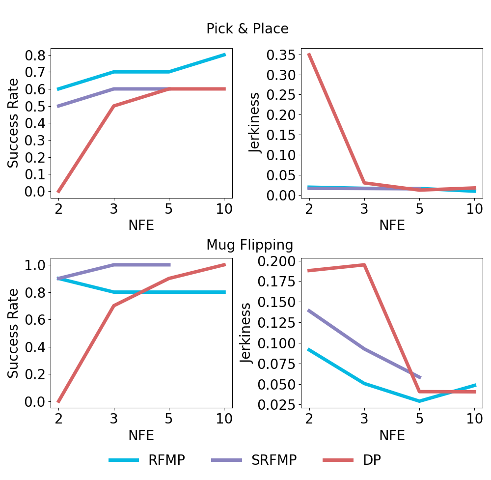
Figure 9: Success rate and predicted actions jerkiness as a function of NFE on the Pick & Place and Mug flipping tasks.

During testing, we systematically place the white mug at $10$ different locations on a semi-grid covering the surface of the yellow sponge. We evaluate the performance of RFMP, SRFMP, and DP as a function of different NFE values, under two metrics: Success rate and prediction smoothness. Figure 9 shows the increased robustness of RFMP and SRFMP to NFE compared to DP. Notably, DP requires more NFEs to achieve a success rate competitive to RFMP and SRFMP, which display high performance with only $2$ NFE. Moreover, DP generated highly jerky predictions when using $2$ NFE. In contrast, RFMP and SRFMP consistently retrieve smooth trajectories, regardless of the NFE.

Our experiments also revealed that slight variations in background and lighting conditions (e.g., cloudy and sunny days), had minimal impact on the policies performance. However, consistent failures were observed when the mug was initially positioned on the right side of the yellow mat, where the robot often obstructs the external camera view when approaching the mug. A multi-camera setting may improve performance on such occlusion cases.

V-D3 Mug Flipping

In this task, a white mug is initially positioned horizontally on a yellow sponge, as shown in Figure 10. The task consists of two stages: First, the robot locates the white mug and grasps it by rotating its end-effector to align with the mug orientation. The robot then places the mug upright on the blue plate. Note that this task demands the robot to execute elaborated rotation trajectories for both grasping and placing. For this task, we collect $50$ demonstrations with the white mug randomly positioned and rotated on the left side of a yellow sponge. Note that we use only the left side as the task requires the robot to operate near its workspace limits, which are prohibitive when the mug is placed on the right side. Furthermore, the end-effector initial pose was also slightly varied across the demonstrations. The policy hyperparameters for this task are provided in Table I.

Figure 10: Mug flipping: The robot rotates its end-effector to align with the white mug’s orientation and subsequently grasps it. It then place the mug upright on the blue plate.

Figure 9 shows the results of evaluating the different considered policies using the same two metrics as the Pick & Place task, namely success rate and trajectory smoothness. Both RFMP and SRFMP are significantly more robust to different NFE in terms of success rate when compared to DP. While the smoothness of RFMP and SRFMP is slightly affected by NFE in this particular task, both methods still outperform DP in this regard. Similarly to the Pick & Place, slight variations on lightning and background had a negligible effect on the performance of the tested policies.

In summary, our findings from both simulated and real-world tasks show that RFMP and SRFMP offer significant advantages over DP. In particular, RFMP and SRFMP achieve faster inference by using fewer NFE without compromising success rates regardless of the observation type. This translates into highly-robust visuomotor policies. Importantly, these advantages do not come at the cost of elaborated training strategies like those used in consistency-based models. In fact, our models demonstrate competitive performance against CP, while being notably easier to train. Regarding the difference between SRFMP and RFMP, the results did not show significant performance gains in terms of success rate and prediction smoothness. Nevertheless, SRFMP shows to be easier to train, achieving higher success rate than RFMP for fewer training epochs (e.g., in Lift, Can, Square tasks).

VI Conclusion

This paper introduced Stable Riemannian Flow Matching Policy (SRFMP), a novel framework that combines the easy training of flow matching with stability-based robustness properties for visuomotor policy learning. SRFMP builds on our extension of stable flow matching to Riemannian manifolds, providing stable convergence of the learned flow to the support of Riemannian target distributions. Our simulated and real-world experiments show that both our previous work on RFMP and its stable counterpart SRFMP outperform diffusion policies and achieve comparable performance to recent distillation-based extensions, while offering advantages in terms of inference speed, ease of training, and robust performance even with limited NFEs and training epochs. Future work will focus on exploring equivariant policy structures to potentially reduce the number of required demonstrations and to improve generalization. Additionally, we aim to investigate multi-modal perception backbones for tackling contact-rich tasks.

References

- [1] J. Urain, A. Mandlekar, Y. Du, M. Shafiullah, D. Xu, K. Fragkiadaki, G. Chalvatzaki, and J. Peters, “Deep generative models in robotics: A survey on learning from multimodal demonstrations,” arXiv preprint arXiv:2408.04380, 2024.
- [2] C. Chi, S. Feng, Y. Du, Z. Xu, E. Cousineau, B. Burchfiel, and S. Song, “Diffusion policy: Visuomotor policy learning via action diffusion,” in Robotics: Science and Systems (R:SS), 2023.
- [3] A. Prasad, K. Lin, J. Wu, L. Zhou, and J. Bohg, “Consistency policy: Accelerated visuomotor policies via consistency distillation,” in Robotics: Science and Systems (R:SS), 2024.
- [4] M. Reuss, M. Li, X. Jia, and R. Lioutikov, “Goal-conditioned imitation learning using score-based diffusion policies,” in Robotics: Science and Systems (R:SS), 2023.
- [5] S.-F. Chen, H.-C. Wang, M.-H. Hsu, C.-M. Lai, and S.-H. Sun, “Diffusion model-augmented behavioral cloning,” in Intl. Conf. on Machine Learning (ICML), 2024.
- [6] Y. Ze, G. Zhang, K. Zhang, C. Hu, M. Wang, and H. Xu, “3d diffusion policy: Generalizable visuomotor policy learning via simple 3d representations,” in Robotics: Science and Systems (R:SS), 2024.
- [7] J. Yang, Z. Cao, C. Deng, R. Antonova, S. Song, and J. Bohg, “Equibot: SIM(3)-equivariant diffusion policy for generalizable and data efficient learning,” in Conference on Robot Learning (CoRL), 2024.
- [8] P. Florence, C. Lynch, A. Zeng, O. A. Ramirez, A. Wahid, L. Downs, A. Wong, J. Lee, I. Mordatch, and J. Tompson, “Implicit behavioral cloning,” in Conference on Robot Learning (CoRL), ser. Proceedings of Machine Learning Research, vol. 164. PMLR, 2022, pp. 158–168.
- [9] N. M. Shafiullah, Z. Cui, A. A. Altanzaya, and L. Pinto, “Behavior transformers: Cloning modes with one stone,” in Neural Information Processing Systems (NeurIPS), 2022.
- [10] A. Mandlekar, D. Xu, J. Wong, S. Nasiriany, C. Wang, R. Kulkarni, L. Fei-Fei, S. Savarese, Y. Zhu, and R. Martín-Martín, “What matters in learning from offline human demonstrations for robot manipulation,” in Conference on Robot Learning (CoRL), 2022, pp. 1678–1690.
- [11] C. Luo, “Understanding diffusion models: A unified perspective,” arXiv preprint arXiv2208.11970, 2022.
- [12] J. Ho, A. Jain, and P. Abbeel, “Denoising diffusion probabilistic models,” Advances in neural information processing systems, vol. 33, pp. 6840–6851, 2020.
- [13] J. Song, C. Meng, and S. Ermon, “Denoising diffusion implicit models,” in Intl. Conf. on Learning Representations (ICLR), 2020.
- [14] C.-W. Huang, M. Aghajohari, J. Bose, P. Panangaden, and A. Courville, “Riemannian diffusion models,” in Neural Information Processing Systems (NeurIPS), 2022.
- [15] Y. Lipman, R. T. Chen, H. Ben-Hamu, M. Nickel, and M. Le, “Flow matching for generative modeling,” in Intl. Conf. on Learning Representations (ICLR), 2022.
- [16] R. T. Chen and Y. Lipman, “Riemannian flow matching on general geometries,” in Intl. Conf. on Learning Representations (ICLR), 2023.
- [17] M. Braun, N. Jaquier, L. Rozo, and T. Asfour, “Riemannian flow matching policy for robot motion learning,” in IEEE/RSJ Intl. Conf. on Intelligent Robots and Systems (IROS), 2024.
- [18] A. Lemme, Y. Meirovitch, M. Khansari-Zadeh, T. Flash, A. Billard, and J. J. Steil, “Open-source benchmarking for learned reaching motion generation in robotics,” Paladyn, Journal of Behavioral Robotics, vol. 6, no. 1, 2015.
- [19] C. I. Sprague, A. Elofsson, and H. Azizpour, “Stable autonomous flow matching,” arXiv preprint arXiv2402.05774, 2024.
- [20] S. Christopher Iliffe, E. Arne, and A. Hossein, “Incorporating stability into flow matching,” in ICML 2024 Workshop on Structured Probabilistic Inference & Generative Modeling, 2024.
- [21] J. LaSalle, “Some extensions of Liapunov’s second method,” IRE Transactions on Circuit Theory, vol. 7, no. 4, pp. 520–527, 1960.
- [22] G. Papamakarios, E. Nalisnick, D. J. Rezende, S. Mohamed, and B. Lakshminarayanan, “Normalizing flows for probabilistic modeling and inference,” Journal of Machine Learning Research, vol. 22, no. 57, pp. 1–64, 2021.
- [23] M. A. Rana, A. Li, D. Fox, B. Boots, F. Ramos, and N. Ratliff, “Euclideanizing flows: Diffeomorphic reduction for learning stable dynamical systems,” in Learning for Dynamics and Control. PMLR, 2020, pp. 630–639.
- [24] S. A. Khader, H. Yin, P. Falco, and D. Kragic, “Learning stable normalizing-flow control for robotic manipulation,” in 2021 IEEE International Conference on Robotics and Automation (ICRA). IEEE, 2021, pp. 1644–1650.
- [25] J. Urain, M. Ginesi, D. Tateo, and J. Peters, “Imitationflow: Learning deep stable stochastic dynamic systems by normalizing flows,” in 2020 IEEE/RSJ International Conference on Intelligent Robots and Systems (IROS). IEEE, 2020, pp. 5231–5237.
- [26] J. Urain, D. Tateo, and J. Peters, “Learning stable vector fields on lie groups,” IEEE Robotics and Automation Letters, vol. 7, no. 4, pp. 12 569–12 576, 2022.
- [27] J. Zhang, H. B. Mohammadi, and L. Rozo, “Learning Riemannian stable dynamical systems via diffeomorphisms,” in 6th Annual Conference on Robot Learning, 2022.
- [28] L. Yang, Z. Zhang, Y. Song, S. Hong, R. Xu, Y. Zhao, W. Zhang, B. Cui, and M.-H. Yang, “Diffusion models: A comprehensive survey of methods and applications,” ACM Comput. Surv., vol. 56, no. 4, 2023.
- [29] M. Janner, Y. Du, J. B. Tenenbaum, and S. Levine, “Planning with diffusion for flexible behavior synthesis,” in Intl. Conf. on Machine Learning (ICML), 2022.
- [30] Z. Wang, J. J. Hunt, and M. Zhou, “Diffusion policies as an expressive policy class for offline reinforcement learning,” in Intl. Conf. on Learning Representations (ICLR), 2023.
- [31] Y. Song, P. Dhariwal, M. Chen, and I. Sutskever, “Consistency models,” in Intl. Conf. on Machine Learning (ICML). PMLR, 2023, pp. 32 211–32 252.
- [32] G. Lu, Z. Gao, T. Chen, W. Dai, Z. Wang, and Y. Tang, “Manicm: Real-time 3d diffusion policy via consistency model for robotic manipulation,” arXiv preprint arXiv:2406.01586, 2024.
- [33] Z. Wang, Z. Li, A. Mandlekar, Z. Xu, J. Fan, Y. Narang, L. Fan, Y. Zhu, Y. Balaji, M. Zhou et al., “One-step diffusion policy: Fast visuomotor policies via diffusion distillation,” arXiv preprint arXiv:2410.21257, 2024.
- [34] A. Tong, K. Fatras, N. Malkin, G. Huguet, Y. Zhang, J. Rector-Brooks, G. Wolf, and Y. Bengio, “Improving and generalizing flow-based generative models with minibatch optimal transport,” Transactions on Machine Learning Research, 2024.
- [35] X. Liu, C. Gong, and Q. Liu, “Flow straight and fast: Learning to generate and transfer data with rectified flow,” in Intl. Conf. on Learning Representations (ICLR), 2022.
- [36] A. J. Bose, T. Akhound-Sadegh, K. Fatras, G. Huguet, J. Rector-Brooks, C.-H. Liu, A. C. Nica, M. Korablyov, M. Bronstein, and A. Tong, “SE(3)-stochastic flow matching for protein backbone generation,” in Intl. Conf. on Learning Representations (ICLR), 2023.
- [37] A. Davtyan, S. Sameni, and P. Favaro, “Efficient video prediction via sparsely conditioned flow matching,” in Proceedings of the IEEE/CVF International Conference on Computer Vision, 2023, pp. 23 263–23 274.
- [38] V. T. Hu, W. Yin, P. Ma, Y. Chen, B. Fernando, Y. M. Asano, E. Gavves, P. Mettes, B. Ommer, and C. G. M. Snoek, “Motion flow matching for human motion synthesis and editing,” arXiv preprint arXiv:2312.08895, 2023.
- [39] X. Zhang, Y. Pu, Y. Kawamura, A. Loza, Y. Bengio, D. L. Shung, and A. Tong, “Trajectory flow matching with applications to clinical time series modeling,” in Neural Information Processing Systems (NeurIPS), 2024.
- [40] H. Lin, O. Zhang, H. Zhao, D. Jiang, L. Wu, Z. Liu, Y. Huang, and S. Z. Li, “PPFlow: Target-aware peptide design with torsional flow matching,” in Intl. Conf. on Machine Learning (ICML), 2024.
- [41] A. H. Liu, M. Le, A. Vyas, B. Shi, A. Tjandra, and W.-N. Hsu, “Generative pre-training for speech with flow matching,” in Intl. Conf. on Learning Representations (ICLR), 2024.
- [42] N. Funk, J. Urain, J. Carvalho, V. Prasad, G. Chalvatzaki, and J. Peters, “Actionflow: Efficient, accurate, and fast policies with spatially symmetric flow matching,” in R:SS workshop: Structural Priors as Inductive Biases for Learning Robot Dynamics, 2024.
- [43] Q. Rouxel, A. Ferrari, S. Ivaldi, and J.-B. Mouret, “Flow matching imitation learning for multi-support manipulation,” arXiv preprint arXiv:2407.12381, 2024.
- [44] E. Chisari, N. Heppert, M. Argus, T. Welschehold, T. Brox, and A. Valada, “Learning robotic manipulation policies from point clouds with conditional flow matching,” in Conference on Robot Learning (CoRL), 2024.
- [45] M. do Carmo, Riemannian Geometry. Birkhäuser Basel, 1992.
- [46] J. M. Lee, Introduction to Riemannian manifolds. Springer, 2018, vol. 2.
- [47] P.-A. Absil, R. Mahony, and R. Sepulchre, Optimization Algorithms on Matrix Manifolds. Princeton University Press, 2007.
- [48] N. Boumal, An introduction to optimization on smooth manifolds. Cambridge University Press, 2023.
- [49] R. T. Chen, Y. Rubanova, J. Bettencourt, and D. K. Duvenaud, “Neural ordinary differential equations,” Advances in neural information processing systems, vol. 31, 2018.
- [50] K. Atkinson, An introduction to numerical analysis. John wiley & sons, 1991.
- [51] J. M. Selig, Geometric fundamentals of robotics. Springer Science & Business Media, 2007.
- [52] F. Merat, “Introduction to robotics: Mechanics and control,” IEEE Journal on Robotics and Automation, vol. 3, no. 2, pp. 166–166, 1987.
- [53] X. Pennec, “Intrinsic statistics on Riemannian manifolds: Basic tools for geometric measurements,” Journal of Mathematical Imaging and Vision, vol. 25, p. 127–154, 2006.
- [54] F. Galaz-Garcia, M. Papamichalis, K. Turnbull, S. Lunagomez, and E. Airoldi, “Wrapped distributions on homogeneous Riemannian manifolds,” arXiv preprint arXiv:2204.09790, 2022.
- [55] D. Q. Mayne and H. Michalska, “Receding horizon control of nonlinear systems,” in IEEE Conference on Decision and Control (CDC), 1988, pp. 464–465.
- [56] J. P. La Salle, “An invariance principle in the theory of stability,” Tech. Rep., 1966.
- [57] X. Mao, “Stochastic versions of the LaSalle theorem,” Journal of differential equations, vol. 153, no. 1, pp. 175–195, 1999.
- [58] E. Perez, F. Strub, H. De Vries, V. Dumoulin, and A. Courville, “Film: Visual reasoning with a general conditioning layer,” in Proceedings of the AAAI conference on artificial intelligence, vol. 32, no. 1, 2018.
- [59] K. V. Mardia and P. E. Jupp, Distributions on Spheres. John Wiley and Sons, Ltd, 1999, ch. 9, pp. 159–192.
- [60] F. Galaz-Garcia, M. Papamichalis, K. Turnbull, S. Lunagomez, and E. Airoldi, “Wrapped distributions on homogeneous riemannian manifolds,” arXiv preprint arXiv:2204.09790, 2022.
- [61] I. Loshchilov and F. Hutter, “Decoupled weight decay regularization,” in Intl. Conf. on Learning Representations (ICLR), 2019.
- [62] B. T. Polyak and A. B. Juditsky, “Acceleration of stochastic approximation by averaging,” SIAM journal on control and optimization, vol. 30, no. 4, pp. 838–855, 1992.
- [63] N. Jaquier, L. Rozo, and T. Asfour, “Unraveling the single tangent space fallacy: An analysis and clarification for applying Riemannian geometry in robot learning,” in IEEE Intl. Conf. on Robotics and Automation (ICRA), 2024, pp. 242–249.