Improving the predictive power of empirical shell-model Hamiltonians

Abstract

We present two developments which enhance the predictive power of empirical shell model Hamiltonians for cases in which calibration data is sparse. A recent improvement in the ab initio derivation of effective Hamiltonians leads to a much better starting point for the optimization procedure. In addition, we introduce a protocol to avoid over-fitting, enabling a more reliable extrapolation beyond available data. These developments will enable more robust predictions for exotic isotopes produced at rare isotope beam facilities and in astrophysical environments.

The nuclear shell model is a ubiquitous framework for interpreting nuclear structure data. In particular, the interacting shell model, or configuration interaction (CI) approach quantitatively reproduces and explains a vast amount of spectroscopic data. These CI calculations require the specification of an effective Hamiltonian. While ab initio methods have made great progress recently in deriving these Hamiltonians from the underlying inter-nucleon interactions, they have not yet achieved the precision obtained with phenomenological Hamiltonians adjusted to data. The gold standard for the phenomenological CI paradigm is the USD family of Hamiltonians, which reproduce spectra with a root-mean-squared deviation of better than 200 keV. In this relatively small model space, the vast amount of available data is more than sufficient to constrain the parameters of the Hamiltonian. In contrast, many of the nuclei that will be studied in the coming decades at rare isotope facilities, including the majority of nuclei relevant for $r$-process nucleosynthesis, will live in larger model spaces where data is sparse. This enhances the importance of maximizing predictive power with minimal data. In addition, the information content of various experimental data is often redundant, in terms of which parameters are constrained; in order to reliably extrapolate beyond the available data it is critical to avoid over-fitting. In this Letter, we (1) demonstrate that an improved ab initio calculation provides a starting point which requires fewer phenomenological adjustments, and (2) utilize a training/testing partitioning scheme to avoid over-fitting.

Microscopic configuration-interaction (CI) calculations for specific regions of nuclei are based on a description in terms of a selected set of shell-model orbitals (the model space) with a Hamiltonian operator

$$H=E_{0}+\sum_{\alpha}\epsilon_{\alpha}\hat{n}_{\alpha}+\sum_{\alpha<\beta,\gamma<\delta}\sum_{J}V_{J}(\alpha\beta;\gamma\delta)\hat{T}_{J}(\alpha\beta;\delta\gamma)$$

that is represented by the energy of the closed core $E_{0}$, single-particle energies (SPE) $\epsilon_{\alpha}$, and two-body matrix elements (TBME) $V_{JT}(\alpha\beta;\gamma\delta)$: In principle, three-body matrix elements could be included, but they dramatically increase the complexity of the problem, and their main effect is to modify the SPE and TBME, so they are generally not treated explicitly. The SPE and TBME can be obtained from a realistic NN (possibly with 3N) interaction, renormalized to the valence space in some way, for example using many-body perturbation theory Hjorth-Jensen1995 , shell model coupled cluster Sun2018 , or the valence-space in-medium similarity renormalization group (VS-IMSRG) sr19 . We use the latter approach in this work, including the effects of 3N interactions via the normal-ordered two-body (NO2B) approximation. This leads to values for $E_{0}$, $\epsilon$ and $V_{J}$ which are nucleus-dependent sr19 .

A commonly applied approximation when optimizing empirical Hamiltonians is to use a nucleus-independent set of SPE and TBME. The TBME may include some smooth mass dependence, e.g. $A^{-0.3}$ sd06 ; mag20 ; fp04 ; jun45 ; jj44b . Within this approximation the SPE and TBME can be used parameters to achieve an improved description of measured binding energies and excitation energies (energy data) with the goal of obtaining improved wavefunctions and improved predictions for new energy data and for other observables.

The singular-value decomposition (SVD) method provides a systematic approach for finding the most important linear combinations of the $N_{p}$ SPE and TBME parameters which can be determined by the data Arima1968 ; Wildenthal1984 ; mag20 . One starts with wavefunctions obtained from a Hamiltonian derived from the best available ab-initio input. With these wavefunctions, the expectation value of the Hamiltonian provides a linear combination of SPE and TBME for each of the $N_{d}$ energy data. The SVD amounts to a diagonalization of the $N_{p}\times N_{p}$ fit matrix solution to $\chi^{2}$ minimization, and provides singular values and associated eigenvectors (linear combinations of SPE and TBME). The largest singular values are associated with the most well determined linear combinations, and smallest singular values are associated with the least well determined combinations. The TBME associated with these least well determined combinations will have some influence on the extrapolations to new energy data and to the calculations of other observables. One must choose a singular value cut-off $N_{c}$. Below the cut off one can use TBME obtained from the best available ab-initio input. This provides a new set of SPE and TBME that can be used to obtain an improved set of wavefunctions. One iterates the SVD fits and the wavefunction calculations until convergence.

Examples of Hamiltonians obtained in this way with protons and neutrons are, USDA/B sd06 and USDC/I mag20 for the $\{0d_{5/2},0d_{3/2},1s_{1/2}\}$ $(sd)$ model space, GPFX1A fp04 for the $\{0f_{7/2},0f_{5/2},1p_{3/2},1p_{1/2}\}$ ($fp$) model space, and JUN45 jun45 and jj44b (Appendix A of jj44b ) for the $\{0f_{5/2},1p_{3/2},1p_{1/2},0g_{9/2}\}$ ($jj44$) model space. For all of these Hamiltonians the root-mean-square-deviation (RMSD) between the calculated and experimental energy data is 150-200 keV. This is to be compared with the results of ab-initio type calculations over the same regions of nuclei where the RMSD is much larger (see Fig. 9 of sr19 for the $sd$ model space). In all of these cases, there is abundant experimental data to constrain the fitted Hamiltonian across the entire model space. However, for very exotic nuclei relevant for rare isotope beam facilities and $r$-process nucleosynthesis, the data will be sparse and strongly biased toward the most stable region of the model space. In such cases, it is possible to overfit to the available data, yielding an Hamiltonians that extrapolates poorly to more exotic nuclei.

In this Letter, we demonstrate that by using an improved ab-initio starting point and by reserving some data for validation, we can improve the predictive power of the resulting Hamiltonian when extrapolating beyond the fit data. For our application, we consider data for low-lying states for all nuclei between ⁷⁸Ni and ¹⁰⁰Sn that can be described by protons in $\{0f_{5/2},1p_{3/2},1p_{1/2},0g_{9/2}\}$ (the $\pi j4$ model space), which requires 4 SPE and 65 TBME with $T=1$ associated with the valence protons. This space has been considered previously with SVD derived Hamiltonians jun45 , jw88 , lisetskiy04 as well as those obtained VS-IMSRG methods Yuan24 . The data we employ consists of 22 ground-state binding energies and 167 excitation energies. The region between ⁹⁰Zr and ¹⁰⁰Sn is well established territory where many wavefunctions are dominated by $\{1p_{1/2},0g_{9/2}\}$ configurations that requires only nine TBME that can be established directly from the energy data talmi60 , cohen64 , aurbach65 , vervier66 , ball72 , gloeckner73 , blomqvist85 . There is new data for nuclei close to ⁷⁸Ni whose structure is dominated by the $\{0f_{5/2},1p_{3/2},1p_{1/2}\}$ subset of orbitals. Importantly, many of the single-particle energies for these orbitals associated with low-lying states in ⁷⁹Cu cu79 and ⁹⁹In in99 are now established . The results from the IMSRG methods discussed below are also shown. In the supplementary material we review the experimental data for nuclei between ⁷⁸Ni and ⁸⁶Kr. This includes a discussion of intruder states that can be attributed to orbital configurations that are not part of the $\pi j4$ model space. These intruder states are excluded from the data set used for the SVD fits.

As a starting point for our fitting procedure, we use Hamiltonians derived with the VS-IMSRG. These are obtained using the EM 1.8/2.0 NN+3N interaction Heb2011 in a harmonic oscillator basis with frequency $\hbar\omega=12$ MeV, truncated to 13 major shells ($2n+l\leq$ $e_{\rm max}=12$). We normal order with respect to the Hartree-Fock ground state of the reference and discard the residual 3N interaction. We then decouple the $\pi j4$ valence space, using the Magnus formulation of the IMSRG. The results labeled IMSRG(2) are obtained with the standard approximation sr19 , truncating all operators at the two-body level throughout the flow, including inside nested commutators. The results labeled IMSRG(3f2) include the recently introduced correction in which intermediate three-body operators arising in nested commutators are incorporated by rewriting the double commutator in a factorized form while maintaining the same computational scaling as the IMSRG(2) approximationHe24 . As in ref. He24 , we include factorized terms with a one-body intermediate during the flow, and include terms with a two-body intermediate at the end of the flow. We perform the procedure for two different references, ⁷⁸Ni and ¹⁰⁰Sn, corresponding to empty and full valence spaces, respectively, and take the average of the two resulting valence space Hamiltonians as our starting point for the fitting procedure.

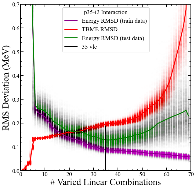
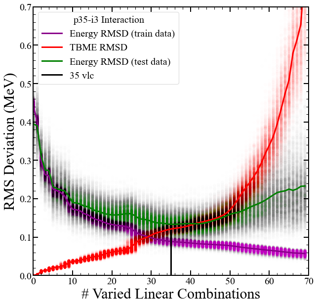
Figure 1: The purple points show the energy-RMSD between theory and experiment as a function of the number of VLC, and the red points show the TBME-RMSD between the IMSRG and fitted Hamiltonians. The lines are the results for the pn-i2 and pn-i3 Hamiltonians. We also show points for the 2000 batches of randomly sampled experimental training data discussed in the text, purple points for the training energy data set, and green points for the predicted data set.

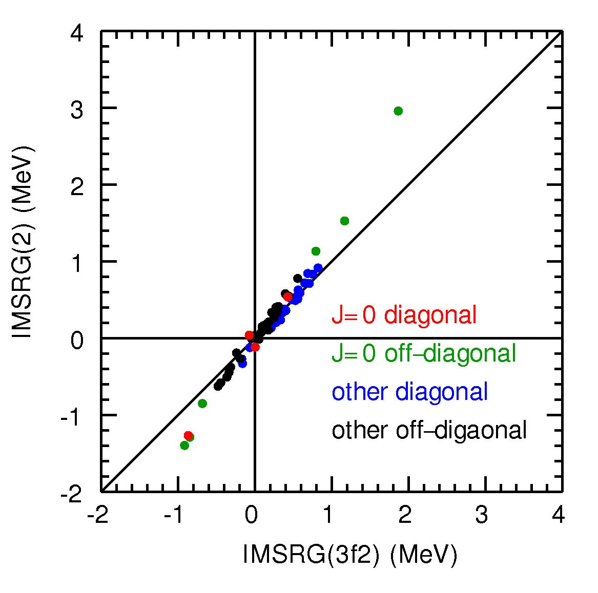
Figure 2: Comparison of the TBME obtained with the two versions of the IMSRG method - the y-axis involves the 2-body truncation and the x-axis involves the factorized approximation. The TBME are colored according to the type of overlap that they describe.

Intuitively, the more realistic the ab initio Hamiltonian is, the less it needs to be modified to produce results that are in agreement with experiment. Shown in FIG. 2 is a comparison of the TBME obtained with the IMSRG(2) and IMSRG(3f2) approximations, indicating the magnitude of the uncertainty due to the many-body truncation. These uncertainties propagate into our effective Hamiltonians, and ultimately the resulting wavefunctions and calculations made with them. The main difference is that the $J=0$, $T=1$ TBME are about 30 percent weaker for IMSRG(3f2) compared to those from IMSRG(2).

FIG. 1 shows the RMSD for the two different IMSRG starting points as a function of the number of VLC. The resulting Hamiltonians will be labeled by $pn\text{--}ia$ where $n$ indicates the number of VLC, and $a$ indicates the ab-initio starting Hamiltonian, $a=2$ for IMSRG(2) and $a=3$ for IMSRG(3f2). The purple line shows the energy-RMSD between the calculated and experimental energy data. Both starting points approach a similar level of energy-RMSD as the number of VLC increase. The major difference between the approach to this threshold is shown by the red points, which shows the RMSD between the fitted and ab-initio TBME. For IMSRG(2) the TBME-RMSD goes above the 200 keV level with 6 VLC, while for the results for IMSRG(3f2) do not reach this level until around 55 VLC. It can also be seen that the energy-RMSD for the fitted data set falls substantially after only one VLC for IMSRG(3f2), while IMSRG(2) requires nearly 15 VLC to reach the same level of accuracy. These results highlight the improvement made for the TBME by the IMSRG(3f2) method. The deviations for each state in the fitted energy data obtained with the p1-i3 and p35-i3 Hamiltonians are shown in FIG. 3.

An essential purpose of these effective Hamiltonians is to achieve some level of predictive power; this is highlighted in FIG. 1. To obtain the scatter of the points around the central fit values as well as the green points in this figure, all of the known experimental data for this model space was randomly partitioned into training (80%) and testing (20%) batches. The training batch was used to vary the parameters of our Hamiltonian, and the testing set was used in the calculation of RMSD - in this way our fitted Hamiltonian is predicting the results of data that it had not seen in the fitting procedure. The sampling process was repeated 2000 times to generate a distribution of calculations for each VLC, and for each set of Hamiltonian parameters. The green curve highlights the predictive capacity of each Hamiltonian as the number of VLC’s is increased. It can be seen that each Hamiltonian approaches an energy-RMSD minimum (a maximum for the predictive power) at about 35 VLC. In fact the RMSD is reasonably small over the range of 15-35 VLC. This is significant because it indicates that we can achieve some benchmark level of predictive power with fewer modifications to our starting Hamiltonian with the factorization method given by He24 . This becomes critically significant when one considers effective Hamiltonians for larger model spaces where producing these effective Hamiltonians and using them to make predictions becomes computationally intensive, or where data is sparse or redundant in terms of constrained parameters.

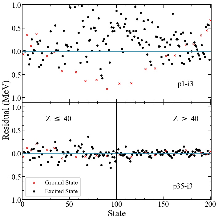
Figure 3: Residual between states calculated from effective Hamiltonian with both (a) 1 VLC and (b) 35 VLC, and corresponding experimental states used to generate the effective Hamiltonian. Both effective Hamiltonians are obtained from the IMSRG(3f2) starting point. We note that the p35-i3 energy differences are larger below $Z=90$ (120 keV) compared those above that (50 keV). The main reason is that the higher-mass data is dominated by only nine TBME associated with the $\{1p_{1/2},0g_{9/2}\}$ orbitals, whereas the lower mass data is dominated by 30 TBME associated with the $\{0f_{5/2},1p_{3/2},1p_{1/2}\}$ orbitals. The supplementary material includes a listing of the experimental and p35-i3 fitted energy data as well as a listing of the p35-i3 SPE and TBME.

The calculations presented in FIG. 5 sampled from the full range of data $28\leq Z\leq 50$, so the predictions are in some sense an interpolation. It is of great interest to also understand the robustness of extrapolations beyond the fit data. To do this, we partition the data so that the training data only contains $Z>36$, and consider the RMSD for $Z\leq 36$. We find that the RMSD in the neutron-rich validation set decreases as the number of VLC is increased, up to 35, where we obtain an RMS of approximately 300 keV. Beyond 35 VLC, the RMSD grows again, indicating that we have begun to over-fit, and extrapolative power deteriorates.

In conclusion, we found that two markedly different starting Hamiltonians can be tuned to produce quite similar results when a robust dataset and fitting method are implemented. The degree to which these starting Hamiltonians must be modified intuitively depends on how successful the initial parameters are at reproducing the known experimental data. The goal is to produce wavefunctions that are realistic and predictive. We conclusively find that the factorized approximation of IMSRG(3f2) given by He24 produces a starting Hamiltonian that requires less modification to reproduce experimental data than ab initio Hamiltonians produced by other methods, meaning that this Hamiltonian is inherently more realistic - a result illustrated clearly in FIG. 1 and FIG. 4. The TBME-RMSD is much smaller with the recently introduced VS-IMSRG(3f2) corrections involving three-body operators. Thus, 3f2 should provide a better input for the linear combinations of parameters that cannot be determined from VLC fits to energy data. In addition, we have demonstrated that utilizing the RMSD from the training/validation partitioning in the fit procedure helps protect against over-fitting, and yields more robust extrapolation to data beyond that used in the fit.

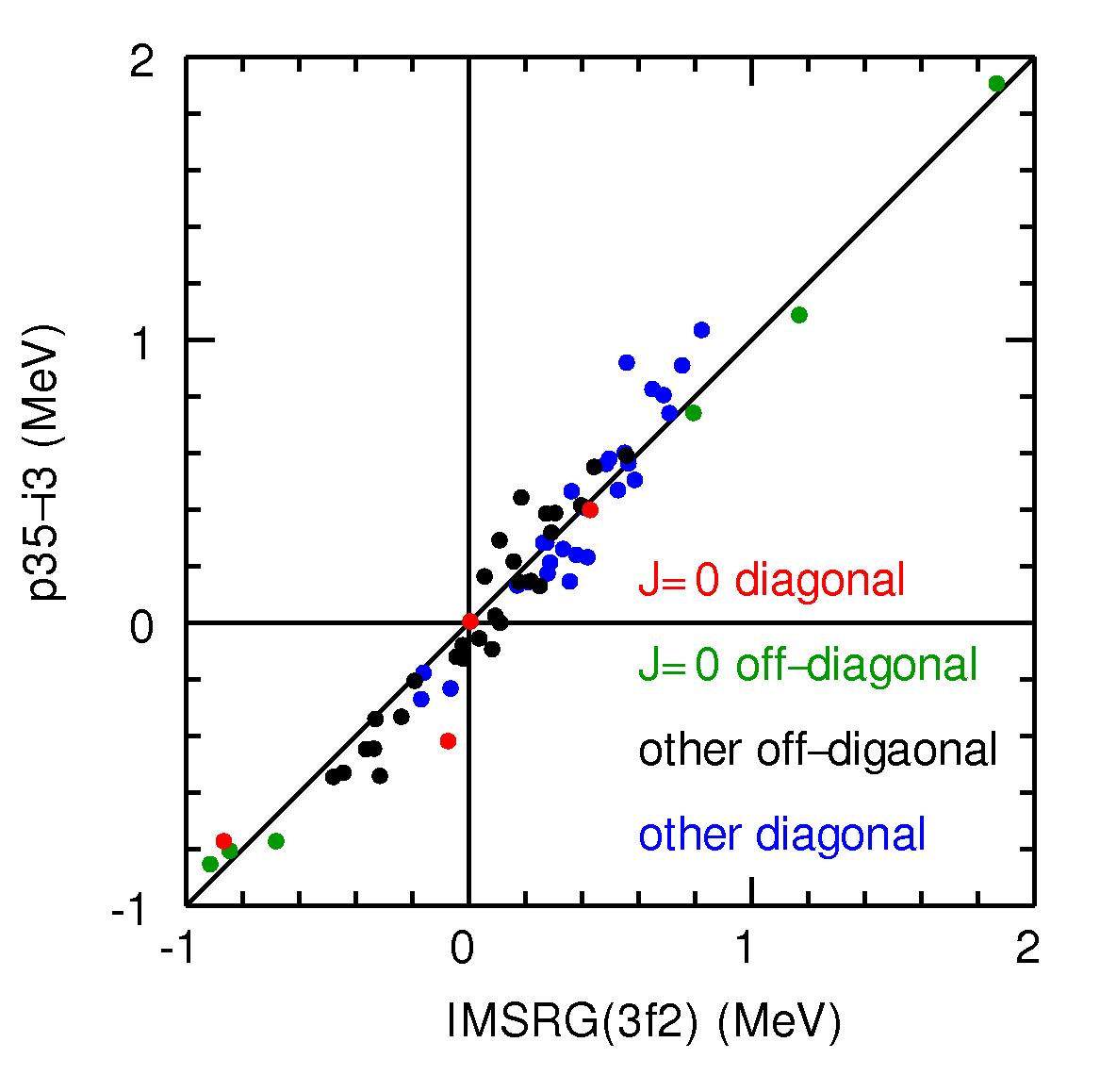
Figure 4: Comparison of the IMSRG(3f2) and p35-i3 TBME.

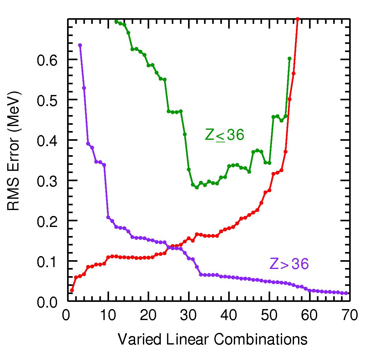
Figure 5: Results obtained when the fitted data set is restricted to $A>86$. See caption to FIG. 1

We acknowledge support from NSF grants PHY-2110365, and PHY-2340834.

I Supplementary Material

I.1 Initial Procedure: $\chi^{2}$ Minimization

Our starting Hamiltonian has a set of parameters $\vec{p}^{s}=(p_{1}^{s},\cdots,p_{N_{p}}^{s})$. This Hamiltonian defines a starting set of eigenvectors $|\phi_{k}^{s}\rangle$ that can be used to calculate the operator overlaps $\beta_{i}^{k}$ so that each associated eigenvalue $\lambda_{k}$ can be calculated in equation $(1)$. Then we seek to minimize the $\ell^{2}$-norm of the residual ($\vec{\chi}$) between the $N_{d}$ measured experimental energies and calculated energy eigenvalues:

$$\underset{\vec{p}\in\mathbb{R}^{N_{p}}}{\textrm{min}}\chi^{2}=\underset{\vec{p}\in\mathbb{R}^{N_{p}}}{\textrm{min}}\sum_{k=1}^{N_{d}}\left(\frac{E_{k}^{exp}-\lambda_{k}(\vec{p})}{\sigma_{k}}\right)^{2}$$

where $\sigma_{k}^{2}=\left(\sigma_{k}^{exp}\right)^{2}+\left(\sigma_{k}^{th}\right)^{2}$. We can reorganize the fitting by expanding $\lambda_{k}$ and defining the expected energy contribution from $H^{1}(\vec{p})$ to be $\epsilon_{k}^{exp}=E_{k}^{exp}-E_{k}^{0}$. Now our $\chi^{2}$ minimization looks like:

$$\underset{\vec{p}\in\mathbb{R}^{N_{p}}}{\textrm{min}}\chi^{2}=\underset{\vec{p}\in\mathbb{R}^{N_{p}}}{\textrm{min}}\sum_{k=1}^{N_{d}}\left(\frac{\epsilon_{k}^{exp}-\epsilon_{k}(\vec{p})}{\sigma_{k}}\right)^{2}$$

We simplify the notation further first by re-expressing our data components $z_{k}^{exp}=\epsilon_{k}^{exp}/\sigma_{k}$ and then considering the model components:

$$z_{k}(\vec{p})=\frac{\epsilon_{k}(\vec{p})}{\sigma_{k}}=\sum_{i=1}^{N_{p}}p_{i}\frac{\beta_{i}^{k}}{\sigma_{k}}$$

We can arrange the components of the experimental data into a data vector $\vec{z}^{exp}=[z_{1}^{exp},\cdots,z_{N_{d}}^{exp}]^{T}$, and similarly for the model components we can represent a model vector through matrix-vector multiplication:

$$\left[\begin{array}[]{c}z_{1}(\vec{p})\\ \vdots\\ z_{N_{d}}(\vec{p})\end{array}\right]=\left[\begin{array}[]{ccc}\beta_{1}^{1}/\sigma_{1}&\cdots&\beta_{N_{p}}^{1}/\sigma_{1}\\ \vdots&\ddots&\vdots\\ \beta_{1}^{N_{d}}/\sigma_{N_{d}}&\cdots&\beta_{N_{p}}^{N_{d}}/\sigma_{N_{d}}\\ \end{array}\right]\left[\begin{array}[]{c}p_{1}\\ \vdots\\ p_{N_{p}}\end{array}\right]$$

If we recognize that $\frac{\beta_{j}^{k}}{\sigma_{k}}=\frac{\partial z_{k}(\vec{p})}{\partial p_{j}}$ then the matrix above must by definition be the transposed Jacobian $(J^{T})$ of the vector-valued function $\vec{z}(\vec{p})=[z_{1}(\vec{p}),\cdots,z_{N_{d}}(\vec{p})]^{T}$. This allows us to re-express our $\chi^{2}$ minimization as:

$$\underset{\vec{p}\in\mathbb{R}^{N_{p}}}{\textrm{min}}\chi^{2}=\underset{\vec{p}\in\mathbb{R}^{N_{p}}}{\textrm{min}}\|\vec{z}^{exp}-J^{T}\vec{p}\|^{2}$$

Minimizing this with respect to each parameter $p_{j}$ gives $N_{p}$ equations of the form:

$$\frac{\partial\chi^{2}}{\partial p_{j}} =2\sum_{k=1}^{N_{d}}\left(\frac{\epsilon_{k}^{exp}-\epsilon_{k}(\vec{p})}{\sigma_{k}}\right)\left(-\frac{1}{\sigma_{k}}\frac{\partial\epsilon_{k}(\vec{p})}{\partial p_{j}}\right)$$

$$=-2\sum_{k=1}^{N_{d}}\left(\frac{\epsilon_{k}^{exp}\beta_{j}^{k}}{\sigma_{k}^{2}}-\sum_{i=1}^{N_{p}}p_{i}\frac{\beta_{i}^{k}\beta_{j}^{k}}{\sigma_{k}^{2}}\right)=0$$

which leaves us with the condition that:

$$\sum_{k=1}^{N_{d}}\frac{\epsilon_{k}^{exp}\beta_{j}^{k}}{\sigma_{k}^{2}}=\sum_{k=1}^{N_{d}}\sum_{i=1}^{N_{p}}p_{i}\frac{\beta_{i}^{k}\beta_{j}^{k}}{\sigma_{k}^{2}}$$

Notice that If we now define the quantities:

$$e_{j}=\sum_{k=1}^{N_{d}}\frac{E_{exp}^{k}\beta_{j}^{k}}{\left(\sigma^{k}\right)^{2}}\quad\textrm{and}\quad G=\left[\begin{array}[]{ccc}\gamma_{11}&\cdots&\gamma_{1p}\\ \vdots&\ddots&\vdots\\ \gamma_{p1}&\cdots&\gamma_{pp}\end{array}\right]$$

where

$$\gamma_{ij}=\sum_{k=1}^{N_{d}}\frac{\beta_{i}^{k}\beta_{j}^{k}}{\left(\sigma^{k}\right)^{2}}=\sum_{k=1}^{N_{d}}\frac{\beta_{j}^{k}\beta_{i}^{k}}{\left(\sigma^{k}\right)^{2}}=\gamma_{ji}\in\mathbb{R}$$

we can rewrite the $N_{p}$ equations as a single vector equation:

$$\vec{e}-G\vec{x}=0\quad\longrightarrow\quad\vec{x}=G^{-1}\vec{e}$$

Since the $G$-matrix is real and symmetric, it is diagonalizable. The step of solving for $\vec{x}$ shown in equation $(2)$ is only possible if G is invertible, meaning that none of the eigenvalues of the $G$-matrix are 0. This process can be used to find a new $\vec{x}$ that can be used to calculate new eigenvalues for the new eigenstates $|\phi_{k}^{\prime}\rangle$, repeating until convergence. $\mathbf{Note:}$ $G^{-1}$ is referred to as the error matrix because its diagonal entries are the square of parameter errors and the off-diagonals are related to correlations between parameters.

SVD Proceedure

The Hamiltonian parameters are often highly correlated, and the fit can be re-expressed in terms of an orthonormal basis of uncorrelated SVD parameters. Since $G$ is real and symmetric, its SVD is identical to an eigendecomposition - the SVD for $G$ and $G^{-1}$ are:

$$G=ADA^{T}\quad\textrm{and}\quad G^{-1}=AD^{-1}A^{T}$$

where:

• $D\in\mathbb{R}^{p\times p}$ is a matrix of diagonal positive elements $D_{ii}>0$.

• $A\in\mathbb{R}^{p\times p}$ is a rotation matrix whose columns form an orthonormal basis of our SVD parameter space.

• $D^{-1}$ is a diagonal matrix whose elements are inverses of the elements of $D$ - i.e. $\left[D^{-1}\right]_{ii}=d_{i}=\frac{1}{D_{ii}}$

With these substitutions in the result of our minimization we have:

$$\vec{x}=AD^{-1}A^{T}\vec{e}\quad\longrightarrow\quad A^{T}\vec{x}=D^{-1}A^{T}\vec{e}$$

Now we express the rotations of $\vec{x}$ and $\vec{e}$

$$\vec{y}=A^{T}\vec{x}\quad\textrm{and}\quad\vec{c}=A^{T}\vec{e}$$

resulting in

$$\vec{y}=D^{-1}\vec{c}\quad\longrightarrow\quad y_{i}=d_{i}c_{i}$$

Here the uncorrelated SVD parameters $y_{i}$ are expressed as a linear combination of the Hamiltonian parameters $x_{i}$ with associated errors $d_{i}$ - explicitly:

$$\vec{y}=A^{T}\vec{x}=\sum_{l=1}^{p}x_{l}\vec{a}_{l}^{T}\quad\longrightarrow\quad y_{i}=\sum_{l=1}^{p}x_{l}\left[A^{T}\right]_{il}$$

where $\vec{a}_{l}^{T}$ is the $l$’th column of $A^{T}$. When $d_{i}$ is large the SVD parameters $y_{i}$ experience a large change from a correspondingly small change in the data $c_{i}$, meaning that the corresponding linear combination of Hamiltonian parameters $y_{i}$ is poorly determined by the given data set. We can establish a cutoff criterion on what is poorly determined linear combination of Hamiltonian parameters $y_{i}$ based on the magnitude of the corresponding $d_{i}$

Fitting Algorithm

1. Starting from the best available Hamiltonian parameters $\vec{x}^{s}$ we construct and diagonalize the $G$-matrix to obtain $D_{ii}$ eigenvalues and the orthonormal basis for our parameter space.

2. Mutually independent SVD parameters $y_{i}$ are determined in the fit from equation $(4)$. Explicitly:

   $$y_{i}=d_{i}c_{i}=d_{i}\sum_{l=1}^{p}e_{l}\left[A^{T}\right]_{il}$$

   Simultaneously, linear combinations of ab initio Hamiltonian parameters are determined from equation $(5)$. Explicitly:

   $$\vec{y}^{*}=A^{T}\vec{x}^{*}\quad\longrightarrow\quad y_{i}^{*}=\sum_{l=1}^{p}x_{l}^{*}\left[A^{T}\right]_{il}$$

3. One defines a cutoff criterion $\delta$, and updated linear combinations $\vec{y}^{a}$ are defined by only adopting well-determined values $y_{i}$ with respect to this cutoff, and leaving ab initio values $y_{i}^{*}$ for the rest:

   $$y_{i}^{a}=\begin{cases}y_{i}\quad&(d_{i}\leq\delta)\\ y_{i}^{*}\quad&(d_{i}>\delta)\end{cases}$$

   The number of well-determined linear combinations is $N_{d}$

4. With the updated set of model parameters $\vec{y}^{a}$ one recovers the Hamiltonian parameters by inverting the rotation:

   $$\vec{x}^{a}=(A^{T})^{-1}\vec{y}^{a}$$

5. This set of Hamiltonian parameters takes the place of $\vec{x}^{s}$ as input to the first step of this algorithm, and is used to obtain the next set of parameters $\vec{x}^{b}$. This process is repeated until convergence.

I.2 Experimental data for the N = 50 isotones

The structure of ⁷⁸Ni has been studied via knock-out reactions and shows a group of excited states between 2.6 and 4.0 MeV ni78 . Levels with spins and parities of 2⁺ and 4⁺ are suggested at 2.60 and 3.18 MeV, respectively. The relatively high excitation of these states indicates that the wavefunction of ⁷⁸Ni is dominates by closed-shell configuration of $Z=28$ for protons and $N=50$ for neutrons. For protons, a $0f_{7/2}$ proton can be moved across the $Z=28$ proton gap into the $0f_{5/2}$ and $1p_{3/2}$ orbitals leading to a multiplet of states with $J^{\pi}$ ranging from 1⁺ to 6⁺. For neutrons, a $0g_{9/2}$ neutron can be moved across the $N=50$ shell gap into the $0d_{5/2}$ orbital, leading to a multiplet of states states from 2⁺ to 7⁺. Also for neutrons, a $1p_{1/2}$ neutron can be moved across $N=50$ into the $0d_{5/2}$ orbital, leading to states with 2^- and 3^-.

The level structure of ⁷⁹Cu has also been studied in knock-out reactions cu79 . Two low-lying levels are proposed at 0.656 and 1.511 MeV with the gamma-decay sequence of 1.511 MeV to 0.656 MeV to the ground state. These experimental energies are compared to shell-model predictions in FIG. 6. All of these predictions give an ordering of 1/2^-, 3/2^- and 5/2^- corresponding to single-particle configurations of $1p_{1/2}$, $1p_{3/2}$ and $0f_{5/2}$, respectively.

The ⁷⁹Cu ground-state spin-parity is not measured. The lighter Cu isotopes are measured to have ⁷¹Cu ($J=3/2$), ⁷³Cu ($J=3/2$), ⁷⁵Cu ($J=5/2$) and ⁷⁷Cu ($J=5/2$) nnds . Shell-model calculations give negative-parity ground states. The energy differences between the lowest levels with $J=3/2^{-}$ and $J=5/2^{-}$ obtained with the JUN45 Hamiltonian jun45 in the $jj44$ model space are shown in Fig. (6). They are compared with experiment for ^69,71,73,75Cu using the energies of the states that are suggested to have $J$ = 3/2 and 5/2 nnds . For ⁷⁹Cu we give the experimental results assumming a ground state and first excited states with $J^{\pi}$ of 5/2^- and 3/2^-, respectively, (solid black line) and 3/2^- and 5/2^-, respectively. (dashed black line). The systematics of these energy differences compared to theory are consistent with the ground state of ⁷⁹Cu having $J^{\pi}$=5/2^-, with the first excited state at 0.656 MeV having $J^{\pi}$=3/2^-. When compared to the shell-model calculations in Fig. (1), the second-excited state at 1.511 MeV is expected to have $J^{\pi}$=1/2^-. The sequence of gamma decays observed in cu79 is consistent with the (1/2^-, 3/2^-, 5/2^-) sequence. In the single-particle model this gives a $1p_{1/2}-1p_{3/2}$ spin-orbit splitting of 0.855 MeV. This smaller the value of 1.66 MeV shown by the MCSM calculations in FIG. 2 of cu79 . The experimental 1/2^- - 3/2^- splitting in in ¹³¹In is suggested to be 988 keV tap16 .

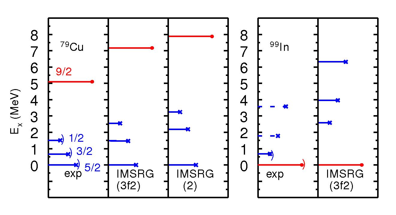
Figure 6: Levels in ⁷⁹Cu and ⁹⁹in. The $J$ value is correlated with the horizontal length of the lines: blue for negative parity and red for positive parity. Experimental levels with suggested $J^{\pi}$ assignments are indicated by ”)” cu79 ; in99 . The 9/2⁺ energy shown in the experimental panel was obtained from our $p35\text{--}i3$ Hamiltonian. The dashed blue lines for ⁹⁹In show excitation energies based on the observations in ¹³¹In in131 . In the $\pi j4$ model space, the states for ⁷⁹Cu are interpreted as single-particle states relative to a ⁷⁸Ni closed shell, and states for ⁹⁹in are interpreted as single-hole states relative to a ¹⁰⁰Sn closed shell. The IMSRG results are based on calculations for ⁷⁸Ni and ¹⁰⁰Sn

Other excited states in ⁷⁹Cu are observed starting at 2.9 MeV. It is natural to understand these as intruder coming from the knockout of an $0f_{7/2}$ proton in ⁸⁰Zn leading to $2p-1h$ states in ⁷⁹Cu. Three transitions at 2.94, 3.88, and 4.30 MeV of about equal intensity that decay directly to the ground state and could represent fragments of the $0f_{7/2}$ hole strength.

The first excited 2⁺ level in ⁸⁰Zn was identified in a Coulomb excitation study at 1.492 MeV zn80w . The Coulex experiment obtains B(E2,$\uparrow$)=20.1(16) e${}^{2}\cdot$fm⁴. Further level structure has been provided from knock-out reactions where a 4${}^{+}_{1}$ level is placed at 1.979 MeV zn80s . In zn80s three other levels are identified at 2.627, 2.820 and 3.174 MeV. The latter two decay only to the 4${}^{+}_{1}$ level. The experimental energies are compared to those from the JUN45 jun45 and MCSM mcsm Hamiltonians in FIG. 4 of zn80s . With only two protons in the $0f_{5/2}$ and $1p_{3/2}$ orbitals beyond ⁷⁸Ni, the maximum positive-parity spin is 4⁺. Lifetimes and B(E2) values have been determined for both the 2$+$ and 4$+$ levels zn80cort .

Level structure for ⁸¹Ga has come from extensive study of the beta decay of the 5/2⁺ ground state of ⁸¹Zn, as well as by both multi-nucleon transfer (MNT) and knock-out reactions. A recent decay scheme was obtained using laser-ionized ⁸¹Zn and has provided the most detail ga81p . The ground-state 5/2^- assignment is supported by laser hyperfine methods ch10 . Two excited 3/2^- levels are identified, along with one clear 9/2^- level and one clear 11/2^- level ga81d . 11/2^- is the highest spin that can be obtained by three protons in the $0f_{5/2}$ and $1p_{3/2}$ orbitals. Levels proposed at higher spins would have to involve either the $0g_{9/2}$ proton orbital, or intruder states coming from the neutron excitations across the $N=50$ shell gap. A possible higher-spin level has been reported by both ga81d and ga81guil at 2.766 MeV that decays to the 11/2^- level. Ref. ga81d also reports on the gamma decay from a level at 3.093 MeV to the 2.766 MeV level, that could have even higher spin. Transitions at 770 keV and 990 keV were observed in (p,2p) reactions that feed into the $11/2^{-}$ level at 1.952 MeV olivPhD .

The basic level structure for ⁸²Ge has been provided by beta-decay of the 2^- ground state of ⁸²Ga ge82alsh , ge82vern , and beta-delayed neutron decay of the 5/2^- ground-state of ⁸³Ga. Also by Coulomb excitation, MNT studies ge82rzac , ge82hwan , ge82carp , ge82sahi , and fission-product gamma-ray studies ge82wilm . Triple coincidences between gamma rays (in MeV) at 1.348 (2⁺), 0.938 (4⁺), and 0.940 (6⁺) establish the yrast sequence. As $6^{+}$ is the highest possible spin for four protons in the $0f_{5/2}$ and $1p_{3/2}$ levels, this level would have to arise from some cross-shell excitation, or involvement of the $0g_{9/2}$ proton orbital. A proposed $7^{+}$ level at 3.948 MeV has been reported thisse23 that decays to the $6^{+}$ level at 3.228 MeV. These $5^{+},6^{+},7^{+}$ states are understood as coming from the excitation of a neutron in the $0g_{9/2}$ orbital into the $1d_{5/2}$ orbital across the $N=50$ shell gap thisse23 ; sie12 . These high-spin particle-hole configurations are also observed in ⁸⁴Se, ⁸⁶Kr and ⁸⁸Sr thisse23 at increasingly higher excitation energy.

The 2${}_{2}^{+}$ MeV level is placed at 2.216 MeV by strong population in all of the decay studies as well as the presence of a 2.216 MeV ground-state transition. The 0${}_{2}^{+}$ level at 2.333 MeV is similarly observed in decay studies with no ground-state transition. Two levels at 2.702 and 2.714 MeV are observed in all of the decay studies, but not observed in the MNT and fission-gamma studies are possible 3⁺ and 1⁺ levels, respectively. Two levels at 2.883 and 2.933 MeV are observed in decay, MNT, and fission studies that decay only to the two lower-energy 4${}_{1}^{+}$ and 4${}_{2}^{+}$ levels and are candidates for 4⁺ and 5⁺ assignments. The B(E2) value for the 1.348 MeV level has been measured by ge82gade .

The level structure of ⁸³As with 33 protons has the most complex structure among the odd-proton $N=50$ isotones. It has 5 valence protons and is exactly half way from $Z=28$ to $Z=38$. The maximum spin available by breaking both pair of protons that occupy the $0f_{5/2}$ and $1p_{3/2}$ orbitals would be 13/2^-. Extensive data exist for the structure of ⁸³As from decay and MNT reaction studies. With 5 protons, the Fermi level has moved up in energy to the point that a 9/2⁺ state associated with the $0g_{9/2}$ proton state should be observed. However, firm identification has remained elusive. A candidate is present at 2.777 MeV that has been assigned (9/2⁺). as83bacz . However, in other studies, no level was assigned as 9/2⁺ as83rezy , se84drou , as83porq . The gamma decay data clearly show low-energy levels that have should have proton configurations, then a gap around 3 MeV where the neutron particle-hole states should be present as83winger . As in ⁸¹Ga, three excited levels in ⁸³As at 0.307, 1.544, and 1.867 MeV are clearly identified as 3/2^-, 9/2^-, and 11/2^-, respectively.

Extensive data are also present for the structure of ⁸⁴Se. Not only from beta decay and multi-nucleon transfer (MNT) studies, but also from the ⁸²Se(t,p)⁸⁴Se 2-neutron transfer reaction. and where cross-shell neutron states are possible, the level density rises rapidly. Levels populated in beta decay were reported by Hoff et. al. se84hoff . High-spin structures have been reported by several groups ge82carp , se84drou .

Three prominent higher-spin levels have been observed at 3.372 [6⁺], 3.639 [5⁺], and 3.704 [6⁺] MeV with the spin and parity assignments derived from Coulex data se84litz , se84mullin , se84knight . A proposed $7^{+}$ level has been identified in several papers at 4.407 MeV. Unlike ⁸²Ge, it is possible to obtain spin and parity of $7^{+}$ by aligning all six protons in the $0f_{5/2}$, $1p_{3/2}$, and $1p_{1/2}$ orbitals thisse23 . Two 0⁺ levels below 3 MeV are identified in both reports at 2.247 and 2.655 keV. Gamma-ray transitions from both of these levels are seen by cross-correlations in the Carpenter data set ge82carp . Three other 0$+$ levels are proposed at 1.967, 2.716, and 2.740 MeV for which no gamma transitions are observed.

The level structure of ⁸⁵Br is quite important for these studies as the data for the spins and parities are on a far firmer basis. Polarized proton pickup in the ⁸⁶Kr(d,³He)⁸⁵Br reaction provide definitive data for the locations of the 3/2^-, 5/2^- and 1/2^- states at 0, 0.345, and 1.191 MeV, respectively. These are associated with $1p_{3/2}$, $0f_{5/2}$, and $1p_{1/2}$ single proton hole states Angular distribution data for the high-spin levels also provide a definite location of the 9/2⁺ level at 1.859 MeV that is associated with proton excitation into the $0g_{9/2}$ orbital. The yrast $9/2^{-}$ and $11/2^{-}$ levels observed in the lower-Z isotones are clearly identified at 1.572 and 2.165 MeV, respectively.

Excellent data are available for the levels of ⁸⁶Kr. The new beta-decay data from the 1^{- 86}Br ground state leads directly to a certain 2^- assignment for the level at 4.316 MeV kr86urban . There is good agreement also for the high-spin levels from studies by two different groups kr86prev , kr86winter . There are Coulex data for the 2⁺ and 3^- levels and a surprising long 3-ns half-life for the 4${}_{1}^{+}$ level.

I.3 Results of the p35-i3 SVD fit.

The first state for each nucleus gives the ground state energy in MeV. The other states for each nucleus are excitation energies in MeV. The table gives the experiment energy, the fitted energy and the energy difference.

Nucleus 2J parity   exp   fitted  difference
  1 Cu 79  5 -  -657.354 -657.437 -0.083
  2 Cu 79  3 -     0.656    0.761  0.105
  3 Cu 79  1 -     1.511    1.550  0.039
  4 Zn 80  0 +  -673.884 -673.802  0.082
  5 Zn 80  4 +     1.497    1.532  0.035
  6 Zn 80  8 +     1.979    2.068  0.089
  7 Zn 80  4 +     2.630    2.490 -0.140
  8 Ga 81  5 -  -687.152 -687.104  0.048
  9 Ga 81  3 -     0.351    0.397  0.046
 10 Ga 81  3 -     0.803    0.615 -0.188
 11 Ga 81  9 -     1.236    1.415  0.179
 12 Ga 81 11 -     1.952    1.937 -0.015
 13 Ge 82  0 +  -702.228 -702.046  0.182
 14 Ge 82  4 +     1.348    1.591  0.243
 15 Ge 82  4 +     2.216    2.332  0.116
 16 Ge 82  8 +     2.288    2.169 -0.119
 17 Ge 82  0 +     2.333    2.463  0.130
 18 Ge 82  8 +     2.524    2.370 -0.154
 19 Ge 82  6 +     2.702    2.702 -0.000
 20 Ge 82  2 +     2.714    2.774  0.060
 21 As 83  5 -  -713.771 -713.688  0.083
 22 As 83  3 -     0.307    0.094 -0.213
 23 As 83  3 -     0.712    0.977  0.265
 24 As 83  1 -     1.194    1.152 -0.042
 25 As 83  9 -     1.543    1.589  0.046
 26 As 83 11 -     1.867    1.788 -0.079
 27 Se 84  0 +  -727.339 -727.205  0.134
 28 Se 84  4 +     1.454    1.781  0.327
 29 Se 84  8 +     2.122    2.199  0.077
 30 Se 84  4 +     2.461    2.457 -0.004
 31 Se 84  0 +     1.967    1.776 -0.191
 32 Se 84  6 +     2.700    2.523 -0.177
 33 Br 85  3 -  -737.255 -737.367 -0.112
 34 Br 85  5 -     0.345    0.425  0.080
 35 Br 85  3 -     0.956    0.901 -0.055
 36 Br 85  1 -     1.191    1.092 -0.099
 37 Br 85  7 -     1.427    1.331 -0.096
 38 Br 85  5 -     1.553    1.477 -0.076
 39 Br 85  9 -     1.571    1.569 -0.002
 40 Br 85  3 -     1.725    1.680 -0.045
 41 Br 85  1 -     1.795    1.643 -0.152
 42 Br 85  9 +     1.859    2.123  0.264
 43 Br 85 11 -     2.165    2.071 -0.094
 44 Br 85 15 +     3.856    3.961  0.105
 45 Kr 86  0 +  -749.234 -749.299 -0.065
 46 Kr 86  4 +     1.565    1.648  0.083
 47 Kr 86  8 +     2.250    2.243 -0.007
 48 Kr 86  4 +     2.349    2.438  0.089
 49 Kr 86  6 +     2.917    3.051  0.134
 50 Kr 86  6 -     3.099    3.275  0.176
 51 Kr 86 10 -     3.935    3.858 -0.077
 52 Kr 86 12 -     4.431    4.345 -0.086
 53 Rb 87  3 -  -757.856 -757.953 -0.097
 54 Rb 87  5 -     0.403    0.436  0.033
 55 Rb 87  1 -     0.845    0.687 -0.158
 56 Rb 87  7 -     1.349    1.575  0.226
 57 Rb 87  3 -     1.390    1.221 -0.169
 58 Rb 87  1 -     1.463    1.399 -0.064
 59 Rb 87  9 +     1.578    1.540 -0.038
 60 Rb 87  5 -     1.678    1.898  0.220
 61 Rb 87 11 +     3.001    3.050  0.049
 62 Rb 87 13 +     3.099    3.082 -0.017
 63 Rb 87 15 +     3.644    3.523 -0.121
 64 Rb 87 17 +     4.151    4.065 -0.086
 65 Sr 88  0 +  -768.468 -768.531 -0.062
 66 Sr 88  4 +     1.836    1.848  0.012
 67 Sr 88  6 -     2.734    2.649 -0.085
 68 Sr 88  0 +     3.156    3.227  0.071
 69 Sr 88  4 +     3.218    3.140 -0.078
 70 Sr 88  6 +     3.635    3.495 -0.140
 71 Sr 88  2 +     3.487    3.457 -0.030
 72 Sr 88 10 -     3.585    3.519 -0.066
 73 Sr 88  8 -     3.953    3.841 -0.112
 74 Sr 88 12 -     4.020    4.072  0.052
 75 Y  89  1 -  -775.547 -775.622 -0.075
 76 Y  89  9 +     0.909    0.878 -0.031
 77 Y  89  3 -     1.507    1.531  0.024
 78 Y  89  5 -     1.745    1.592 -0.153
 79 Y  89  5 +     2.222    1.994 -0.228
 80 Y  89  7 +     2.530    2.546  0.016
 81 Y  89 11 +     2.567    2.499 -0.068
 82 Y  89  9 +     2.622    2.770  0.148
 83 Y  89 13 +     2.893    2.842 -0.051
 84 Y  89 13 -     3.343    3.231 -0.112
 85 Y  89 15 -     4.132    4.078 -0.054
 86 Y  89 17 -     4.450    4.450 -0.000
 87 Y  89 19 -     4.839    4.973  0.134
 88 Zr 90  0 +  -783.897 -783.920 -0.023
 89 Zr 90  0 +     1.761    1.760 -0.001
 90 Zr 90  4 +     2.186    2.200  0.014
 91 Zr 90 10 -     2.319    2.286 -0.033
 92 Zr 90  8 -     2.739    2.695 -0.044
 93 Zr 90  6 -     2.748    2.703 -0.045
 94 Zr 90  8 +     3.077    3.071 -0.006
 95 Zr 90  4 +     3.309    3.446  0.137
 96 Zr 90 12 +     3.448    3.402 -0.046
 97 Zr 90 16 +     3.589    3.505 -0.084
 98 Zr 90 18 +     5.248    5.170 -0.078
 99 Zr 90 20 +     5.644    5.476 -0.168
100 Nb 91  9 +  -789.052 -789.117 -0.065
101 Nb 91  1 -     0.105    0.097 -0.008
102 Nb 91  5 -     1.187    1.194  0.007
103 Nb 91  3 -     1.313    1.361  0.048
104 Nb 91  7 +     1.581    1.558 -0.023
105 Nb 91  3 -     1.613    1.568 -0.045
106 Nb 91  9 +     1.637    1.635 -0.002
107 Nb 91  9 -     1.790    1.864  0.074
108 Nb 91 13 -     1.984    2.001  0.017
109 Nb 91 17 -     2.034    2.038  0.004
110 Nb 91 13 +     2.290    2.273 -0.017
111 Nb 91 11 -     2.413    2.459  0.046
112 Nb 91 15 -     2.660    2.749  0.089
113 Nb 91 17 +     3.110    3.148  0.038
114 Nb 91 21 +     3.466    3.518  0.052
115 Mo 92  0 +  -796.511 -796.471  0.040
116 Mo 92  4 +     1.510    1.560  0.050
117 Mo 92  8 +     2.283    2.296  0.013
118 Mo 92  0 +     2.520    2.515 -0.005
119 Mo 92 10 -     2.527    2.467 -0.060
120 Mo 92 12 +     2.612    2.551 -0.061
121 Mo 92 16 +     2.760    2.656 -0.104
122 Mo 92  6 -     2.850    2.893  0.043
123 Tc 93  9 +  -800.598 -800.598 -0.000
124 Tc 93  1 -     0.392    0.382 -0.010
125 Tc 93  7 +     0.681    0.758  0.077
126 Tc 93  5 -     1.408    1.414  0.006
127 Tc 93 13 +     1.434    1.473  0.039
128 Tc 93 11 +     1.516    1.551  0.035
129 Tc 93 13 -     2.185    2.172 -0.013
130 Tc 93 17 +     2.185    2.230  0.045
131 Tc 93 17 -     2.185    2.170 -0.015
132 Tc 93 21 +     2.535    2.521 -0.014
133 Tc 93 21 -     3.281    3.291  0.010
134 Tc 93 25 -     3.888    3.965  0.077
135 Ru 94  0 +  -806.864 -806.781  0.083
136 Ru 94  4 +     1.431    1.473  0.042
137 Ru 94  8 +     2.187    2.184 -0.003
138 Ru 94 12 +     2.498    2.464 -0.034
139 Ru 94  8 +     2.503    2.472 -0.031
140 Ru 94 10 -     2.624    2.569 -0.055
141 Ru 94 16 +     2.644    2.551 -0.093
142 Ru 94  0 +     2.995    3.049  0.054
143 Ru 94 14 -     3.658    3.607 -0.051
144 Rh 95  9 +  -809.910 -809.879  0.031
145 Rh 95  1 -     0.543    0.560  0.017
146 Rh 95  7 +     0.680    0.706  0.026
147 Rh 95  5 +     1.180    1.232  0.052
148 Rh 95 13 +     1.351    1.401  0.050
149 Rh 95 11 +     1.430    1.479  0.049
150 Rh 95 17 +     2.068    2.134  0.066
151 Rh 95 17 -     2.236    2.232 -0.004
152 Rh 95 21 +     2.450    2.453  0.003
153 Rh 95 21 -     3.243    3.289  0.046
154 Rh 95 25 +     3.724    3.848  0.124
155 Rh 95 25 -     3.909    3.954  0.045
156 Pd 96  0 +  -815.042 -814.964  0.078
157 Pd 96  4 +     1.415    1.412 -0.003
158 Pd 96  8 +     2.099    2.127  0.028
159 Pd 96 12 +     2.424    2.369 -0.055
160 Pd 96 16 +     2.531    2.482 -0.049
161 Pd 96 10 -     2.649    2.615 -0.034
162 Pd 96 14 +     3.184    3.180 -0.004
163 Pd 96 20 +     3.784    3.815  0.031
164 Ag 97  9 +  -817.052 -817.063 -0.011
165 Ag 97  7 +     0.716    0.694 -0.022
166 Ag 97 13 +     1.290    1.321  0.031
167 Ag 97 11 +     1.418    1.512  0.094
168 Ag 97  9 +     1.673    1.750  0.077
169 Ag 97 15 +     2.020    2.082  0.062
170 Ag 97 17 +     2.053    2.124  0.071
171 Ag 97 21 +     2.343    2.401  0.058
172 Cd 98  0 +  -821.073 -821.087 -0.014
173 Cd 98  4 +     1.395    1.371 -0.024
174 Cd 98  8 +     2.082    2.090  0.008
175 Cd 98 12 +     2.280    2.281  0.001
176 Cd 98 16 +     2.428    2.430  0.002
177 Cd 98 10 -     2.627    2.619 -0.008
178 In 99  9 +  -822.155 -822.201 -0.046
179 In 99  1 -     0.671    0.734  0.063
180 In 99  3 -     1.780    1.782  0.002
181 In 99  5 -     3.580    3.585  0.005
182 Sn 00  0 +  -825.163 -825.190 -0.027

I.4 The p35-i3 Hamiltonian

All numbers are in units of MeV. The orbitals are labeled by $k$ with $k=1$ for $0f_{5/2}$, $k=2$ for $1p_{3/2}$, $k=3$ for $1p_{1/2}$, and $k=4$ for $0g_{9/2}$. SPE(1) = -14.8729 SPE(2) = -14.1118, SPE(3) = -13.3233, and SPE(4) = -9.7056. The table contains $k_{1},k_{2},k_{3},k_{4},J$ and TBME$(k_{1},k_{2},k_{3},k_{4}J,T=1)$.

 1 1 1 1  0  -0.4231
 1 1 2 2  0  -0.9062
 1 1 3 3  0  -0.9527
 1 1 4 4  0   1.7602
 2 2 2 2  0   0.0985
 2 2 3 3  0  -0.6757
 2 2 4 4  0   1.2092
 3 3 3 3  0   0.4232
 3 3 4 4  0   0.7347
 4 4 4 4  0  -0.7997
 1 2 1 2  1   0.7977
 1 2 2 3  1  -0.0102
 2 3 2 3  1   0.7258
 1 1 1 1  2   0.4175
 1 1 1 2  2  -0.2325
 1 1 1 3  2  -0.4466
 1 1 2 2  2  -0.2462
 1 1 2 3  2  -0.3913
 1 1 4 4  2   0.3924
 1 2 1 2  2   0.8217
 1 2 1 3  2   0.2397
 1 2 2 2  2   0.2777
 1 2 2 3  2   0.3862
 1 2 4 4  2  -0.6077
 1 3 1 3  2   0.1329
 1 3 2 2  2   0.0384
 1 3 2 3  2  -0.4775
 1 3 4 4  2   0.5542
 1 4 1 4  2   0.0421
 2 2 2 2  2   0.2882
 2 2 2 3  2  -0.4163
 2 2 4 4  2   0.6484
 2 3 2 3  2   0.1423
 2 3 4 4  2   0.3348
 4 4 4 4  2  -0.1620
 1 2 1 2  3   0.8950
 1 2 1 3  3  -0.1740
 1 3 1 3  3   1.1166
 1 4 1 4  3   0.2328
 1 4 2 4  3   0.1689
 2 4 2 4  3  -0.2489
 1 1 1 1  4   0.5909
 1 1 1 2  4  -0.0808
 1 1 4 4  4   0.0712
 1 2 1 2  4   0.2474
 1 2 4 4  4  -0.6290
 1 4 1 4  4   0.5752
 1 4 2 4  4   0.1236
 1 4 3 4  4  -0.1368
 2 4 2 4  4   0.6199
 2 4 3 4  4  -0.1014
 3 4 3 4  4   0.6132
 4 4 4 4  4   0.2891
 1 4 1 4  5   0.2415
 1 4 2 4  5   0.0179
 1 4 3 4  5  -0.4179
 2 4 2 4  5   0.1877
 2 4 3 4  5   0.2897
 3 4 3 4  5   0.1333
 1 4 1 4  6   0.5584
 1 4 2 4  6   0.4964
 2 4 2 4  6   0.8076
 4 4 4 4  6   0.4062
 1 4 1 4  7  -0.3052
 4 4 4 4  8   0.5553

References

- (1) M. Hjorth-Jensen, T. T. S. Kuo and E. Osnes, Phys. Rep. 261, 125 (1995).
- (2) Z. H. Sun, T. D. Morris, G. Hagen, G. R. Jansen, and T. Papenbrock, Phys. Rev. C 98, 054320 (2018).
- (3) S. R. Stroberg, H. Hergert, S. K. Bogner, and J. D. Holt, Annu. Rev. Nucl. Part. Sci. 2019. 69, 307 (2019).
- (4) B. A. Brown and W. A. Richter, Phys. Rev. C 7 4, 034315 (2006).
- (5) A. Magilligan and B. A. Brown, Phys. Rev. C 101, 064312 (2020).
- (6) M. Honma, T. Otsuka, B. A. Brown and T. Mizusaki, Phys. Rev. C 69, 034335 (2004).
- (7) M. Honma, T. Otsuka, T. Mizusaki, and M. Hjorth-Jensen, Phys. Rev. C 80, 064323 (2009).
- (8) S. Mukhopadhyay, B. P. Crider, B. A. Brown, S. F. As hley, A. Chakraborty, A. Kumar, E. E. Peters, M. T. McEllistrem, F. M. Prados-Estevez, and S. W. Yates, Phys. Rev. C 95, 014327 (2017).
- (9) A. Arima, S. Cohen, R. D. Lawson, and M. H. MacFarlane, Nucl. Phys. A108, 94 (1968).
- (10) B. H. Wildenthal, Prog. Part. Nucl. Phys. 11, 5 (1984).
- (11) X. Ji and B. H. Wildenthal, Phys. Rev. C 37, 1256 (1988).
- (12) A. F. Lisetskiy, B. A. Brown, M. Horoi and H. Grawe, Phys. Rev. C 70, 044314 (2004).
- (13) Q. Yuan and B. S. Hu, Phys. Lett. B 858, 139018 (2024).
- (14) I. Talmi and I. Unna, Nucl. Phys. 19, 225 (1960).
- (15) S. Cohen, R. D. Lawson, M. H. Macfarlane, and M. Soga, Phys. Lett. 10, 195 (1964).
- (16) N. Auerbach and I. Talmi, Nucl. Phys. 64, 458 (1965).
- (17) J. Vervier, Nucl. Phys. 75, 17 (1966).
- (18) J. B. Ball, J. B.McGrory, and J. S. Larsen, Phys. Lett. 41B, 581 (1972).
- (19) D. H. Gloeckner and F. J. D. Serduke, Nucl. Phys . A220, 4 (1973).
- (20) J. Blomqvist and L. Rysdtrom, Phys. Scr. 31, 31 (1985).
- (21) L. Olivier et. al., Phys. Rev. Lett. 119, 19201 (2017).
- (22) L. Nies et al., Phys. Rev. Lett. 131, 022502 (2023).
- (23) V. Vaquero et al, Phys. Rev. Lett. 124, 022501 (2020).
- (24) K. Hebeler, S. K. Bogner, R. J. Furnstahl, A. Nogga, and A. Schwenk Phys. Rev. C 83, 031301(R) (2011)
- (25) B. C. He and S. R. Stroberg, Phys. Rev. C 110, 044317 (2024).
- (26) R. Taniuchi et. al., Nature 569, 53 (2019).
- (27) J. Taprogge et. al. Eur. Phys. J. A (2016) 52: 347
- (28) National Nuclear Data Center
- (29) J. Van de Walle, Phys. Rev. Lett. 107, 142501 (2007).
- (30) Y. Shiga et al., Phys. Rev. C 93, 024320 (2016).
- (31) MCSM
- (32) M. L. Cortes et. al., Phys. Rev. C 97, 044315 (2018).
- (33) V. Paziy et. al., Phys. Rev. C 102, 014329 (2020).
- (34) B. Cheal et. al., Phys. Rev. Lett. 104, 252502 (2010).
- (35) J. Dudouet et. al., Phys. Rev. C 100, 011301(R) (2019).
- (36) L. Olivier., Ph.D. thesis, University Paris-Saclay, (2017)
- (37) Guillaume Maquart, Physique Nucleaire Experimental, Universtite de Lyon, (2017).
- (38) M. F. Alshudifat et. al., Phys.Rev. C 93, 044325 (2016).
- (39) D. Verney et. al., Phys. Rev. C 76, 054312 (2007).
- (40) T. Rzaca-Urban, W. Urban, J. L. Durell, A. G. Smith, and I. Ahmad, Phys. Rev. C 76, 027302 (2007).
- (41) K. Hwang, J. H. Hamilton, A. V. Ramayya, N. T. Brewer, Y. X. Luo, J. O. Rasmussen, and S. J. Zhu, Phys. Rev. C 84, 024305 (2011).
- (42) M. P. Carpenter et al., Physics Division Annual Report 2006, Argonne National Labortory.
- (43) E. Sahin, G. de Angelis, G. Duchene, T. Faul, A. Gadeaa, A. F. Lisetskiy, D. Ackermann, A. Algora, S. Aydinhi, F. Azaiez et al., Nucl. Phys. A 893, 1 (2012).
- (44) D. Wilmsen, Thesis, Universite de Caen Normandie (2017).
- (45) Thisse, D., Lebois, M., Verney, D. et al. Eur. Phys. J. A 59, 153 (2023)
- (46) K. Sieja and F. Nowacki, Phys. Rev. C 85, 051301(R) (2012).
- (47) A. Gade et al., Phys. Rev. C 81, 064326 (2010).
- (48) P. Baczyk, W. Urban, D. Zlotowska, M. Czerwinski, T. Rzaca-Urban, A. Blanc, M. Jentschel, P. Mutti, U. Koster, T. Soldner, G. de France, G. Simpson, and C. A. Ur, Phys. Rev. C 91, 047302 (2015)
- (49) K. Rezynkina et al., Phys. Rev. C 106, 014320 (2022).
- (50) F. Drouet, G. S. Simpson, A. Vancraeyenest, G. Gey, G. Kessedjian, T. Malkiewicz, M. Ramdhane, C. Sage, G. Thiamova, T. Grahn et al., EPJ Web Conf. 62, 01005 (2013), DOI: 10.1051/epjconf/20136201005
- (51) M. G. Porquet et al., Phys. Rev. C 84, 054305 (2011)
- (52) J. A. Winger, J. C. Hill, F. K. Wohn, R. L. Gill, X. Ji, and B.H. Wildenthal, Phys. Rev. C 38, 285 (1988).
- (53) P. Hoff and B. Fogelberg, Nucl. Phys. A 368, 210 (1981).
- (54) J. Litzenger et. al., Phys. Rev. C 92, 064322 (2015).
- (55) S. M. Mullins, D. L. Watson, H. T. Fortune, Phys. Rev. C 37, 587 (1988).
- (56) J. D. Knight, C. J. Orth, W. T. Leland and A. B. Tucker, Phys. Rev. C 9, 1467 (1974).
- (57) W. Urban et. al., Phys. Rev. C 94, 044328 (2016).
- (58) A. Prevost et. al., Eur. Phys. J A 22, 391 (2004).
- (59) G. Winter, L. Funke, R. Schwengner, H. Prade, R. Wirowski, N. Nicolay, A. Dewald, P. von Brentano, Z. Phys. A 343, 369 (1992).