A Unified Convergence Analysis Framework of the Energy-stable ETDRK3 Schemes for the No-Slope-Selection Thin Film Model

Abstract

The recent studies [21] and [22] introduce two temporally third-order accurate exponential time differencing Runge–Kutta (ETDRK3) numerical schemes, both of which can be expressed in a unified one-parameter formulation and have been proven to unconditionally preserve the discrete energy dissipation law for the no-slope-selection (NSS) equation in the epitaxial thin film growth model. However, no study has provided the theoretical proof of the convergence of such schemes. Consequently, this paper establishes a unified framework for the space-time convergence analysis of these energy-stable schemes. By employing Fourier pseudo-spectral discretization in space and the inner product technique, we derive a rigorous Fourier eigenvalue analysis, which provides a detailed optimal convergence rate and error estimate in the $\ell^{\infty}(0,T;H_{h}^{1})\cap\ell^{2}(0,T;H_{h}^{3})$ norm. The primary challenge is addressing the complex nonlinear terms in the NSS equation. Fortunately, this challenge could be resolved through careful eigenvalue bound estimates for various operators. The proposed analysis builds on the approach in [J. Sci Comput, 81 (2019), pp. 154–185], while significantly optimizing and simplifying the proof process.

MSC Classification]65T50, 65L04, 65M12, 65M20

1 Introduction

In this paper, we consider a two-dimensional (2-D) epitaxial thin film growth equation, which corresponds to the $L^{2}$ gradient flow associated with the following energy functional:

$$E(u):=\int_{\Omega}\Bigl{(}-\frac{1}{2}\ln(1+|\nabla u|^{2})+\frac{\varepsilon^{2}}{2}|\Delta u|^{2}\Bigr{)}\,\mathrm{d}\mathbf{x},$$ (1.1)

where $\Omega=(0,L_{x})\times(0,L_{y}),~{}u:\Omega\to\mathbb{R}^{2}$ is a periodic height function, and $\varepsilon$ is a constant. Since the logarithm term $-\frac{1}{2}\ln(1+|\nabla u|^{2})$ has no relative minima, there are no energetically favored values for $|\nabla u|$, which means that there is no slope selection mechanism in the epitaxial growth dynamics. The second term, which is quadratic, represents the isotropic surface diffusion effect. In turn, the chemical potential becomes the following variational derivative of the energy:

$$\mu:=\delta_{u}E=\nabla\cdot\Bigl{(}\frac{\nabla u}{1+|\nabla u|^{2}}\Bigr{)}+\varepsilon^{2}\Delta^{2}u,$$

and the no-slope-selection (NSS) equation stands for the $L^{2}$ gradient flow,

$$\partial_{t}u=-\mu=-\nabla\cdot\Bigl{(}\frac{\nabla u}{1+|\nabla u|^{2}}\Bigr{)}-\varepsilon^{2}\Delta^{2}u,$$ (1.2)

in which the fourth-order term in (1.2) models the surface diffusion and the nonlinear second-order term describes the Ehrlich-Schowoebel effect [1, 2, 3, 4]. Under the periodic boundary condition, the NSS equation (1.2) is mass conservative, i.e.,

$$\frac{\mathrm{d}}{\mathrm{d}t}\int_{\Omega}u(\mathbf{x},t)=0.$$ (1.3)

Up to the present, significant efforts have been devoted to the design and analysis of numerical schemes for the NSS equation; see the relevant literature [5, 6, 7, 8, 10, 9, 12, 11, 13, 14], among others. In particular, numerical schemes with high-order accuracy and energy stability are of particular interest, owing to the long-time nature of the gradient flow coarsening process. For example, based on the convex-concave decomposition of the energy, the convex splitting framework introduced by Eyre [15] has led to the development of a number of unconditionally energy-stable schemes; see, e.g., [5, 6, 7, 9, 13] and the references therein. Meanwhile, exponential time differencing (ETD) methods have emerged as a popular research direction in recent years. Ju et al. [16] first introduced unconditionally energy-stable first- and second-order ETD multi-step (ETDMS) schemes by introducing a stabilization constant. Then, Wang et al. [7, 17, 18] incorporated various Douglas-Dupont stabilizing terms to analyze the energy stability of second-, third-, and even higher-order stabilized ETDMS schemes, along with long-time error estimates. Due to the multi-step nature of these schemes, the total energy is always composed of the original terms and some regularized terms, referred to as the “modified energy." While the corresponding theoretical foundation is rigorous, there is a preference for retaining the original energy as it more closely reflects the physical reality of the problem.

Motivated by this, Sun and Zhou [20] adopted explicit single-step time integration to propose a second-order unconditionally energy-stable ETDRK (ETDRK2) scheme. Furthermore, they established error estimates and proved unconditional original energy stability without the need for the Lipschitz assumption on the nonlinear terms. Very recently, the studies [21] and [22] proposed third-order ETDRK (ETDRK3) schemes and successfully proved the discrete energy dissipation law for phase-field models, including the NSS equation (1.2).

For the temporal convergence analysis and error estimates of the ETD-based schemes, the authors [16, 20] derived the first- and second-order temporal $\ell^{\infty}(0,T;\ell^{2})$ convergence result with useful mathematical tools, such as

$$\|e^{n+1}\|_{2}\leq C\tau^{k},\quad(k=1,2),$$ (1.4)

in which $e^{n+1}$ stands for the numerical error in the next time step, $C$ is some constant with subscript of the relevant parameters, and $\tau$ is the time-step size. To obtain a higher regularity result, Cheng et al. [7] presented the following third-order temporal convergence result, in the $\ell^{\infty}(0,T;H_{h}^{1})\cap\ell^{2}(0,T;H_{h}^{3})$ norm:

$$\|\nabla_{\mathcal{N}}e^{\ell}\|_{2}+\Big{(}\varepsilon^{2}\tau\sum_{m=1}^{\ell}\|\nabla_{\mathcal{N}}\Delta_{\mathcal{N}}e^{m}\|_{2}^{2}\Big{)}^{1/2}\leq C\tau^{3}.$$ (1.5)

Motivated by the framework constructed by [7], this study aims to provide a rigorous convergence analysis for the two existing ETDRK3 schemes. To begin, we identify the core structure of the two schemes, which can be expressed in a unified Butcher-like formulation, with a single degree of freedom determined by one parameter. The formulation is then decomposed into two distinct stages: in the first stage, the linear part is integrated exponentially, introducing an intermediate variable; while in the second stage, an explicit single-step interpolation is applied to handle the nonlinear part. Error estimates are finally derived for both stages, with a thorough application of linearized stability analysis in the second stage.

A key challenge in the analysis of this high-order ETDRK formulation arises from the involvement of various global and inverse operators within the algorithm. To establish a uniform bound for these operators, we carefully estimate the eigenvalues of the operators, as well as those of their compositions. By applying an aliasing error control technique to the $\ell^{\infty}(0,T;H_{h}^{1})$ error estimate, we are also able to derive the spatial convergence rate and naturally establish the fully-discrete error estimates. In contrast to the approach in [7], we shall adopt a single-step analysis strategy, namely, the analysis of each time step of the model scheme is independent of the others. In addition, to finish the complete proof, the authors in [7] used mathematical induction, that is, their convergence analysis requires the assumption that $\|\nabla_{\mathcal{N}}\Delta_{\mathcal{N}}e^{m}\|_{2}\leq 1$ holds (cf. Proposition 3.2 in [7]), and this condition is recovered at the time instant $t^{n+1}$. In contrast, our approach does not rely on any assumption or recovery, which significantly simplifies the proof. Another important point to note is that, owing to the structure of the one-parameter ETDRK3 formulation, the most operators we use are considerably simpler than those in [7], which make the analysis more accessible to readers.

The rest of this paper is organized as follows. In Section 2, we present the fully-discrete numerical schemes, which combine Fourier pseudo-spectral spatial discretization with two third-order accurate exponential time differencing Runge-Kutta methods for time integration. We also supplement the discrete mass conservation law. Section 3 contains the main convergence theorem and its corresponding proof, as well as the definitions of various operators in Fourier space. In the following section, we briefly provide numerical evidence that supports the theoretical results from Section 3. Finally, we conclude with some remarks.

2 Review of the energy-stable ETDRK3 Fourier pseudo-spectral schemes

2.1 Fourier pseudo-spectral discretization

Consider $\Omega=(0,L)^{2}$. For simplicity of presentation, we let $N$ be a positive integer, and $N_{x}=N_{y}=N$ and $N\cdot h=L$. We also set the number of grid points in each direction as $N=2K+1$, and the case for an even $N$ could also be similarly treated. We compute the variables at the regular numerical grid $\Omega_{\mathcal{N}}:=\{(x_{p},y_{q})|x_{p}=ph,~{}y_{q}=qh,~{}0\leq p,\,q\leq N\}$. Denote $u_{e}$ as the exact solution of (1.2), $u(t)=u_{e}(\cdot,t)|_{\Omega_{\mathcal{N}}}$ be the restriction of the exact solution on $\Omega_{\mathcal{N}}$, $\tau$ be the time step $\frac{T}{N_{t}}$, and $t_{i}=i\tau$ for $0\leq i\leq N_{t}$. Let $H_{\mathrm{per}}^{m}(\Omega)=\{v\in H^{m}(\Omega)|v~{}\text{is periodic}\}$, and $\mathcal{M}_{\mathcal{N}}$ be the space of 2-D periodic grid functions on $\Omega_{\mathcal{N}}$. In this paper, we denote $C$ (such as (1.4) and (1.5)) one generic constant which may depend on $\varepsilon$, the solution $u$, the stabilization constant $\kappa$, and the total time $T$, but is independent of the mesh size $h$ and the time-step size $\tau$.

The discrete Fourier expansion for a periodic grid function $f\in\mathcal{M}_{\mathcal{N}}$ is defined as

$$f_{p,q}=\sum_{\ell,m=-K}^{K}\hat{f}_{\ell,m}\mathrm{e}^{2\pi\mathrm{i}(\ell x_{p}+my_{q})/L},\quad\mbox{with}~{}\hat{f}_{\ell,m}=\frac{1}{N^{2}}\sum_{p,q=0}^{N-1}f_{p,q}\mathrm{e}^{-2\pi\mathrm{i}(\ell x_{p}+y_{q})/L}.$$ (2.1)

Then, the first- and second-order discrete spatial partial derivatives in the $x$-direction are approximated by:

$$(D_{x}f)_{p,q}=\sum_{\ell,m=-K}^{K}\frac{2k\pi\mathrm{i}}{L}\hat{f}_{\ell,m}\mathrm{e}^{2\pi\mathrm{i}(\ell x_{p}+my_{q})/L},\quad(D_{x}^{2}f)_{p,q}=\sum_{\ell,m=-K}^{K}-\frac{4k\pi^{2}}{L^{2}}\hat{f}_{\ell,m}\mathrm{e}^{2\pi\mathrm{i}(\ell x_{p}+my_{q})/L}.$$

The differentiation operators in the $y$-direction ($D_{y}$ and $D_{y}^{2}$) could be similarly defined. For any $f,g\in\mathcal{M}_{\mathcal{N}}$, and $(f_{1},f_{2})^{T}\in\mathcal{M}_{\mathcal{N}}\times\mathcal{M}_{\mathcal{N}}$, the discrete gradient, divergence and Laplacian could be defined as follows:

$$\nabla_{\mathcal{N}}f=\begin{pmatrix}D_{x}f\\ D_{y}f\end{pmatrix},\quad\nabla_{\mathcal{N}}\cdot\begin{pmatrix}f_{1}\\ f_{2}\end{pmatrix}=D_{x}f_{1}+D_{y}f_{2},\quad\Delta_{\mathcal{N}}f=D_{x}^{2}f+D_{y}^{2}f.$$

We also need to introduce the discrete $L^{2}$ inner product $\langle\cdot,\cdot\rangle$ and norm $\|\cdot\|_{2}$ to measure the discrete differentiation operators defined above,

$$\langle f,g\rangle=h^{2}\sum_{i,j=1}^{2N}f_{ij}g_{ij},\qquad\qquad\quad\|f\|_{2}=\sqrt{\langle f,f\rangle}.$$

Furthermore, a detailed calculation shows that the following formulas of summation by parts are valid at the discrete level. [28, 29]

$$\left\langle f,\nabla_{\mathcal{N}}\cdot\begin{pmatrix}g_{1}\\ g_{2}\end{pmatrix}\right\rangle=-\left\langle\nabla_{\mathcal{N}}f,\begin{pmatrix}g_{1}\\ g_{2}\end{pmatrix}\right\rangle,\quad\langle f,\Delta_{\mathcal{N}}g\rangle=-\langle\nabla_{\mathcal{N}}f,\nabla_{\mathcal{N}}g\rangle=\langle\Delta_{\mathcal{N}}f,g\rangle.$$

In turn, the spatial discretization of equation (1.2) becomes: Given $u_{0}\in\mathcal{M}_{\mathcal{N}}$, find $u:[0,T]\to\mathcal{M}_{\mathcal{N}}$ such that

$$\left\{\begin{aligned} &\frac{\mathrm{d}u}{\mathrm{d}t}=-L_{\kappa}u+N_{\kappa}(u),\quad t\in(0,T],\\ &u(0)=u(0),\end{aligned}\right.$$ (2.2)

where the operator $L_{\kappa}=\varepsilon^{2}\Delta_{\mathcal{N}}^{2}-\kappa\Delta_{\mathcal{N}}$ that is symmetric negative definite on $\mathcal{M}_{\mathcal{N}}$, and the nonlinear term $N_{\kappa}(u)=-\kappa\Delta_{\mathcal{N}}u-\nabla_{\mathcal{N}}\cdot\left(\frac{\nabla_{\mathcal{N}}u}{1+|\nabla_{\mathcal{N}}u|^{2}}\right)$. Further, we denote $g_{\kappa}(u)=\kappa\nabla_{\mathcal{N}}u+\frac{\nabla_{\mathcal{N}}u}{1+|\nabla_{\mathcal{N}}u|^{2}}$, so that $N_{\kappa}(u)=-\nabla_{\mathcal{N}}\cdot g_{\kappa}(u)$. The following Calculus-style inequality has been proven in an existing work [16].

Lemma 2.1.

Denote a mapping $\beta:\,\mathbb{R}^{2}\to\mathbb{R}^{2}$ that $\beta(\bm{v})=\frac{\bm{v}}{1+|\bm{v}|^{2}}$. Then, we have

$$|\beta(\bm{v})-\beta(\bm{w})|\leq|\bm{v}-\bm{w}|,\quad\forall\bm{v},\,\bm{w}\in\mathbb{R}^{2}.$$

Also, we introduce the following $\ell^{2}$ estimate [7], which will be needed in the later analysis.

Lemma 2.2.

For any two grid functions $f_{1}$ and $f_{2}$, we have

$$\|g_{\kappa}(f_{1})-g_{\kappa}(f_{2})\|_{2}\leq(\kappa+1)\|\nabla_{\mathcal{N}}(f_{1}-f_{2})\|_{2}.$$ (2.3)

Moreover, to overcome the difficulty caused by an appearance of aliasing error in the nonlinear term, we introduce a periodic extension of a grid function and a Fourier collocation interpolation operator defined in [7].

Definition 2.1.

For any periodic grid function $f$ defined over a uniform 2-D numerical grid, we denote $f_{N}$ as its periodic extension. In more details, suppose that the grid function $f$ has a discrete Fourier expansion as (2.1), its continuous extension (projection) onto $\mathcal{P}_{K}$ (the space of trigonometric polynomials of degree at most $K$) is given by

$$f_{N}(\bm{x})=\sum_{\ell,m=-K}^{K}\hat{f}_{\ell,m}\mathrm{e}^{2\pi\mathrm{i}(\ell x+my)/L}.$$

Meanwhile, for any periodic continuous function $\bm{f}$, which may contain larger wave length, its collocation interpolation operator is defined as

$$\bm{f}_{p,q} =\sum_{\ell,m=-K}^{K}\big{(}\hat{f}_{c}\big{)}_{\ell,m}\mathrm{e}^{2\pi\mathrm{i}(\ell x_{p}+my_{q})/L}$$

$$P_{c}^{N}\bm{f}_{N}(\bm{x}) =\sum_{\ell,m=-K}^{K}\big{(}\hat{f}_{c}\big{)}_{\ell,m}\mathrm{e}^{2\pi\mathrm{i}(\ell x+my)/L},$$

in which the Fourier collocation coefficients $(\hat{f}_{c})_{\ell,m}$ could be obtained by discrete Fourier transformation. Notice that $\hat{f}_{c}$ may not be the Fourier coefficients of $\bm{f}$, due to the truncation and aliasing errors. The following two lemmas [23, 24, 25] are necessary for the later unified convergence analysis where the definition of the norm $\|\cdot\|_{H^{m}}$ is omit here for simplicity of presentation.

Lemma 2.3.

For any $\phi\in\mathcal{P}_{mK}$ in dimension $d$, we have

$$\big{\|}P_{c}^{N}\phi\big{\|}_{H^{k_{0}}}\leq(\sqrt{m})^{d}\|\phi\|_{H^{k_{0}}},\quad\forall k_{0}\in\mathbb{Z},~{}k_{0}\geq 0.$$

Lemma 2.4.

As long as $f$ and all its derivatives (up to $m$-th order) are continuous and periodic on $\Omega$, the convergence of the derivatives of the interpolation is given by

$$\|f-P_{c}^{N}f\|_{H^{k}}\leq C\|f\|_{H^{m}}h^{m-k},\quad\mbox{for}~{}0\leq k\leq m,~{}m>\frac{d}{2}.$$

2.2 Derivation of the time-stepping integrators

To define ETDRK methods, we introduce the functions

$$\varphi_{k}(z)=\int_{0}^{1}\mathrm{e}^{(1-s)z}\frac{s^{k-1}}{(k-1)!}\mathrm{d}s>0,\quad k\geq 1,$$

which satisfy the recursion relation ($z\neq 0$):

$$\varphi_{k}(z)=\frac{\varphi_{k-1}(z)-\frac{1}{(k-1)!}}{z},~{}k\geq 1,\quad\text{with}~{}\varphi_{0}(z)=\mathrm{e}^{z}.$$

More precisely, when $k=1,2$, the two $\varphi$-functions read as follows,

$$\varphi_{1}(z)=\frac{1-\mathrm{e}^{-z}}{z},\qquad\varphi_{2}(z)=\frac{\mathrm{e}^{-z}-1+z}{z^{2}},$$

and the vital properties holds for the later analysis.

Lemma 2.5.

1. $\varphi_{i}$ is decreasing for $i=0,1,2$;

2. $\forall x>0,~{}\mbox{it holds that}~{}0<\varphi_{1}(z)\leq 1$, $0<\varphi_{2}(z)\leq\frac{1}{2}$, and $\big{|}\frac{\varphi_{2}(z)}{\sqrt{\varphi_{1}(z)}}\big{|}\leq\frac{1}{2}$.

We outline an three-stage stabilization ETDRK3 formulation for (2.2) in the form:

$$\left\{\begin{aligned} &u_{n,0}=u^{n},\\ &u_{n,i}=\varphi_{0}(c_{i}\tau L_{\kappa})u^{n}+\tau\sum_{j=0}^{i-1}a_{i,j}(\tau L_{\kappa})N_{\kappa}(u_{n,j}),\quad i=1,2,3,\\ &u^{n+1}=u_{n,3}.\end{aligned}\right.$$ (2.4)

According to the consistency analysis, Hochbruck and Ostermann [26] found the following one-parameter family of third-order methods:

$$\begin{array}[]{c|ccc}c_{0}&&&\\ c_{1}&a_{1,0}(\tau L_{\kappa})&&\\ c_{2}&a_{2,0}(\tau L_{\kappa})&a_{2,1}(\tau L_{\kappa})&\\ \hline\cr c_{3}&a_{3,0}(\tau L_{\kappa})&a_{3,1}(\tau L_{\kappa})&a_{3,2}(\tau L_{\kappa})\end{array}=\begin{array}[]{c|cccc}0&&&\\ c_{1}&c_{1}\varphi_{1,1}&&\\ \frac{2}{3}&\frac{2}{3}\varphi_{1,2}-\frac{4}{9c_{1}}\varphi_{2,2}&\frac{4}{9c_{1}}\varphi_{2,2}&\\ \hline\cr 1&\varphi_{1}-\frac{3}{2}\varphi_{2}&0&\frac{3}{2}\varphi_{2}\end{array},$$ (2.13)

where $\varphi_{i,j}(\tau L_{\kappa}):=\varphi_{i}(c_{j}\tau L_{\kappa})$. By selecting different parameter values, one can obtain the following two third-order ETDRK schemes:

• [21] ETDRK3-1 ($c_{1}=\frac{2}{3}$):

  $$\left\{\begin{aligned} u_{n,1}=&\varphi_{0}\bigl{(}\frac{2}{3}\tau L_{\kappa}\bigr{)}u^{n}+\frac{2}{3}\tau\varphi_{1}\bigl{(}\frac{2}{3}\tau L_{\kappa}\bigr{)}N_{\kappa}(u^{n}),\\ u_{n,2}=&u_{n,1}+\frac{2}{3}\tau\varphi_{2}\bigl{(}\frac{2}{3}\tau L_{\kappa}\bigr{)}\bigl{(}N_{\kappa}(u_{n,1})-N_{\kappa}(u^{n})\bigr{)},\\ u^{n+1}=&\varphi_{0}(\tau L_{\kappa})u^{n}+\tau\varphi_{1}(\tau L_{\kappa})N_{\kappa}(u^{n})+\frac{3}{2}\tau\varphi_{2}(\tau L_{\kappa})\bigl{(}N_{\kappa}(u_{n,2})-N_{\kappa}(u^{n})\bigr{)}.\end{aligned}\right.$$ (2.14)

• [22] ETDRK3-2 ($c_{1}=\frac{4}{9}$):

  $$\left\{\begin{aligned} u_{n,1}=&\varphi_{0}\bigl{(}\frac{4}{9}\tau L_{\kappa}\bigr{)}u^{n}+\frac{4}{9}\tau\varphi_{1}\bigl{(}\frac{4}{9}\tau L_{\kappa}\bigr{)}N_{\kappa}(u^{n}),\\ u_{n,2}=&\varphi_{0}(\frac{2}{3}\tau L_{\kappa})u^{n}+\frac{2}{3}\tau\varphi_{1}\bigl{(}\frac{2}{3}\tau L_{\kappa}\bigr{)}N_{\kappa}(u^{n})+\tau\varphi_{2}(\frac{2}{3}\tau L_{\kappa})\bigl{(}N_{\kappa}(u_{n,1})-N_{\kappa}(u^{n})\bigr{)},\\ u^{n+1}=&\varphi_{0}(\tau L_{\kappa})u^{n}+\tau\varphi_{1}(\tau L_{\kappa})N_{\kappa}(u^{n})+\frac{3}{2}\tau\varphi_{2}(\tau L_{\kappa})\bigl{(}N_{\kappa}(u_{n,2})-N_{\kappa}(u^{n})\bigr{)}.\end{aligned}\right.$$ (2.15)

To prove the mass conservation of the ETDRK3-1 (2.14) and ETDRK3-2 (2.15) schemes, we first introduce the following lemma [27].

Lemma 2.6.

Let $g$ be an analytic function defined on the spectrum of $M\in\mathbb{C}^{d\times d}$; that is, the values $g^{(i)}(\lambda_{i})(0\leq j\leq n_{i}-1,\,1\leq i\leq d)$ exists, where $\{\lambda_{i}\}_{i=1}^{d}$ are the eigenvalues of $M$, and $n_{i}$ is the order of the largest Jordan block where $\lambda_{i}$ appears. Then it holds that

1. $g(M)$ commutes with $M$;

2. $g(M^{T})=g(M)^{T}$;

3. the eigenvalues of $g(M)$ are $g(\lambda_{i}),~{}1\leq i\leq d$;

4. $g(P^{-1}MP)=P^{-1}g(M)P$ for any non-singular matrix $P\in\mathbb{C}^{d\times d}$;

5. for any $P,Q\in\mathbb{C}^{d\times d}$, $\mathrm{e}^{(P+Q)t}=\mathrm{e}^{Pt}\mathrm{e}^{Qt}=\mathrm{e}^{Qt}\mathrm{e}^{Pt}$ iff $PQ=QP$;

6. $\frac{\mathrm{d}}{\mathrm{d}t}(\mathrm{e}^{Mt})=M\mathrm{e}^{Mt}=\mathrm{e}^{Mt}M$.

Proposition 2.1 (Discrete mass conservation).

The ETDRK3-1 (2.14) and ETDRK3-2 (2.15) schemes preserves unconditionally mass conservation in the discrete sense; that is,

$$\overline{u^{n+1}}=\overline{u^{n}}:=\frac{1}{|\Omega|}\int_{\Omega}u^{n}\mathrm{d}\mathbf{x},\quad 0\leq n\leq N_{t}-1.$$

Proof.

We can rewrite the third equation of (2.14) or (2.15) as follows:

$$\begin{aligned} u^{n+1}-u^{n}=&\bigl{(}\mathrm{e}^{-\tau L_{\kappa}}-I\bigr{)}u^{n}+L_{\kappa}^{-1}\bigl{(}I-\mathrm{e}^{-\tau L_{\kappa}}\bigr{)}N_{\kappa}(u^{n})\\ &+\frac{3}{2}L_{\kappa}^{-1}(\tau L_{\kappa})^{-1}\bigl{(}\mathrm{e}^{-\tau L_{\kappa}}-I+\tau L_{\kappa}\bigr{)}\bigl{(}N_{\kappa}(u_{n,2})-N_{\kappa}(u^{n})\bigr{)}.\end{aligned}$$ (2.16)

We introduce two functions $g_{1}$ and $g_{2}:\mathbb{R}\to\mathbb{R}$, defined by

$$g_{1}(a)=1-\mathrm{e}^{-\tau a},\qquad g_{2}(a)=\frac{\mathrm{e}^{-\tau a}-1+\tau a}{\tau a}.$$

It follows that for any $a>0$, we have $0<g_{1}(a)<1$ and $0<g_{2}(a)<\frac{1}{2}$. Furthermore, we define the operators $B_{1}$ and $B_{2}$ as

$$B_{1}=g_{1}(L_{\kappa}),\qquad B_{2}=g_{2}(L_{\kappa}),$$

so that (2.16) becomes

$$u^{n+1}-u^{n}=B_{1}\bigl{(}-u^{n}+L_{\kappa}^{-1}N_{\kappa}(u^{n})\bigr{)}+\frac{3}{2}L_{\kappa}^{-1}B_{2}\bigl{(}N_{\kappa}(u_{n,2})-N_{\kappa}(u^{n})\bigr{)}.$$ (2.17)

By using the lemma and the fact that $L_{\kappa}$ is symmetric and positive definite, we conclude that both $B_{1}$ and $B_{2}$ are symmetric, positive definite, and commute with $L_{\kappa}$ and $L_{\kappa}^{-1}$. Now, by taking the discrete $L^{2}$ inner product of (2.17) with $v_{0}\equiv 1$, we obtain

$$\overline{u^{n+1}}-\overline{u^{n}}=\langle u^{n+1}-u^{n},1\rangle=\big{\langle}L_{\kappa}^{-1}N_{\kappa}(u^{n})-u^{n},B_{1}v_{0}\big{\rangle}+\frac{3}{2}\big{\langle}L_{\kappa}^{-1}\bigl{(}N_{\kappa}(u_{n,2})-N_{\kappa}(u^{n})\bigr{)},B_{2}v_{0}\big{\rangle}.$$

From the definitions of $B_{1}$ and $B_{2}$, we derive the following expressions:

$$B_{1}=I-\mathrm{e}^{-\tau L_{\kappa}}=\tau L_{\kappa}-\frac{1}{2}(\tau L_{\kappa})^{2}+\frac{1}{6}(\tau L_{\kappa})^{3}+\cdots,$$

$$B_{2}=(\tau L_{\kappa})^{-1}\bigl{(}\mathrm{e}^{-\tau L_{\kappa}}-I+\tau L_{\kappa}\bigr{)}=\frac{1}{2}\tau L_{\kappa}-\frac{1}{6}(\tau L_{\kappa})^{2}+\frac{1}{24}(\tau L_{\kappa})^{3}+\cdots.$$

Therefore, we conclude that $B_{1}v_{0}=B_{2}v_{0}=0$, which completes the proof. ∎

3 Optimal rate convergence analysis of the fully-discrete scheme

In this section, we present a unified convergence analysis framework for the third-order formulation (2.4). For clarity, we first provide the explicit form of the formulation:

$$u_{n,1} =\varphi_{0}(c_{1}\tau L_{\kappa})u^{n}+c_{1}\tau\varphi_{1}(c_{1}\tau L_{\kappa})N_{\kappa}(u^{n}),$$ (3.1)

$$u_{n,2} =\varphi_{0}(\frac{2}{3}\tau L_{\kappa})u^{n}+\frac{2}{3}\tau\varphi_{1}(\frac{2}{3}\tau L_{\kappa})N_{\kappa}(u^{n})+\frac{4}{9c_{1}}\tau\varphi_{2}(\frac{2}{3}\tau L_{\kappa})\big{(}N_{\kappa}(u_{n,1})-N_{\kappa}(u^{n})\bigr{)},$$ (3.2)

$$u^{n+1} =\varphi_{0}(\tau L_{\kappa})u^{n}+\tau\varphi_{1}(\tau L_{\kappa})N_{\kappa}(u^{n})+\frac{3}{2}\tau\varphi_{2}(\tau L_{\kappa})\bigl{(}N_{\kappa}(u_{n,2})-N_{\kappa}(u^{n})\bigr{)}.$$ (3.3)

The global existence of weak solution, strong solution, and smooth solution for the NSS equation (1.2) has been established in [3]. In more details, a global-in-time estimate of $L^{\infty}(0,T;H^{m})\cap L^{2}(0,T;H^{m+2})$ for the phase variable was proved, assuming initial data in $H^{m}$, for any $m\geq 2$. Therefore, with an initial data with sufficient regularity, the exact solution is assumed to preserve a regularity of class $\mathcal{R}$:

$$u_{e}\in\mathcal{R}:=C^{3}(0,T;H^{3})\cap L^{\infty}(0,T;H^{M_{0}}),\quad M_{0}=\max\{17,m_{0}+5\}.$$

Define $U_{N}(\cdot,t):=\mathcal{P}_{N}u_{e}(\cdot,t)$, the (spatial) Fourier projection of the exact solution into $\mathcal{B}^{K}$, the space of trigonometric polynomials of degree to and including $K$. The following projection approximation is standard: if $\phi_{e}\in L^{\infty}(0,T;H_{\mathrm{per}}^{\ell}(\Omega))$, for some $\ell\in\mathbb{N}$,

$$\|U_{N}-u_{e}\|_{L^{\infty}(0,T;H^{m})}\leq Ch^{\ell-k}\|u_{e}\|_{L^{\infty}(0,T;H^{\ell})},\quad\forall 0\leq k\leq\ell.$$

By $U_{N}^{m}$ we denote $U_{N}(\cdot,t^{m})$, with $t^{m}=m\cdot\tau$. Since $U_{N}\in\mathcal{P}_{K}$, the mass conservative property is available at the discrete level:

$$\overline{U_{N}^{m}}=\frac{1}{|\Omega|}\int_{\Omega}U_{N}(\cdot,t_{m})\mathrm{d}\mathbf{x}=\frac{1}{|\Omega|}\int_{\Omega}U_{N}(\cdot,t_{m-1})\mathrm{d}\mathbf{x}=\overline{U_{N}^{m-1}},\quad\forall m\in\mathbb{N}.$$

On the other hand, the solution of the scheme (2.14) or (2.15) is also mass conservative at the discrete level (as given by Proposition 2.1); that is,

$$\overline{u^{m}}=\overline{u^{m-1}},\quad\forall m\in\mathbb{N}.$$

Meanwhile, we denote $U^{m}$ as the interpolation values of $U_{N}$ at discrete grid points at time instant $t^{m}$: $U_{p,q}^{m}:=U_{N}(x_{p},y_{q},t^{m})$. As indicated before, we use the mass conservative projection for the initial solution:

$$u_{p,q}^{0}=U_{p,q}^{0}:=U_{N}(x_{p},y_{q},t=0).$$

The error grid function is defined as

$$e^{m}:=U^{m}-u^{m},\quad\forall m\in\mathbb{N}.$$ (3.4)

Therefore, it follows that $\overline{e^{m}}=0$, $\forall m\in\mathbb{N}$. For the introduced third-order accurate scheme (3.1)-(3.3), the convergence result is stated below.

Theorem 3.1.

Given initial data $U_{\mathcal{N}}^{0}\in H_{\mathrm{per}}^{M_{0}}(\Omega)$ with periodic boundary conditions, suppose that the unique solution for the NSS equation is of regularity class $\mathcal{R}$. Then, provided that $\tau$ and $h$ are sufficiently small, for all positive integers $k$, such that $\tau\cdot k\leq T$, the following convergence estimate is valid:

$$\|\nabla_{\mathcal{N}}e^{k}\|_{2}+\Bigl{(}\varepsilon^{2}\tau\sum_{j=1}^{k}\|G_{\mathcal{N}}^{1,3,(0)}\nabla_{\mathcal{N}}\Delta_{\mathcal{N}}e^{j}\|_{2}^{2}\Bigr{)}^{\frac{1}{2}}\leq C(\tau^{3}+h^{m_{0}}),$$ (3.5)

where $G_{\mathcal{N}}^{1,3,(0)}$ is a specific operator defined in (3.21).

We will begin by proving the convergence result of the ETDRK3 formulation (3.1)-(3.3) for the NSS equation (1.2) and putting the complete process into Section 3.2-Section 3.4.

3.1 Preliminaries

For the Fourier projection solution $U_{N}$ and its interpolation $U$, a careful consistency analysis implies that

$$U_{n,1} =\varphi_{0}(c_{1}\tau L_{\kappa})U^{n}+c_{1}\tau\varphi_{1}(c_{1}\tau L_{\kappa})N_{\kappa}(U^{n}),$$ (3.6)

$$U_{n,2} =\varphi_{0}(\frac{2}{3}\tau L_{\kappa})U^{n}+\frac{2}{3}\tau\varphi_{1}(\frac{2}{3}\tau L_{\kappa})N_{\kappa}(U^{n})+\frac{4}{9c_{1}}\tau\varphi_{2}(\frac{2}{3}\tau L_{\kappa})\bigl{(}N_{\kappa}(U_{n,1})-N_{\kappa}(U^{n})\bigr{)},$$ (3.7)

$$U^{n+1} =\varphi_{0}(\tau L_{\kappa})U^{n}+\tau\varphi_{1}(\tau L_{\kappa})N_{\kappa}(U^{n})+\frac{3}{2}\tau\varphi_{2}(\tau L_{\kappa})\bigl{(}N_{\kappa}(U_{n,2})-N_{\kappa}(U^{n})\bigr{)}+\tau\zeta^{n},$$ (3.8)

with $\|\nabla_{\mathcal{N}}\zeta^{n}\|\leq C(\tau^{3}+h^{m_{0}})$. Notice that the profiles $U_{n,1}$ and $U_{n,2}$ are constructed, based on the exact interpolation solution $U^{n}$ at the previous time step. In turn, subtracting the numerical algorithm (3.1)-(3.3) from the consistency estimate (3.6)-(3.8) gives

$$e_{n,1} =\varphi_{0}(c_{1}\tau L_{\kappa})e^{n}+c_{1}\tau\varphi_{1}(c_{1}\tau L_{\kappa})\tilde{N}_{\kappa}(e^{n}),$$ (3.9)

$$e_{n,2} =\varphi_{0}(\frac{2}{3}\tau L_{\kappa})e^{n}+\frac{2}{3}\tau\varphi_{1}(\frac{2}{3}\tau L_{\kappa})\tilde{N}_{\kappa}(e^{n})+\frac{4}{9c_{1}}\tau\varphi_{2}(\frac{2}{3}\tau L_{\kappa})\bigl{(}\tilde{N}_{\kappa}(e_{n,1})-\tilde{N}_{\kappa}(e^{n})\bigr{)},$$ (3.10)

$$e^{n+1} =\varphi_{0}(\tau L_{\kappa})e^{n}+\tau\varphi_{1}(\tau L_{\kappa})\tilde{N}_{\kappa}(e^{n})+\frac{3}{2}\tau\varphi_{2}(\tau L_{\kappa})\bigl{(}\tilde{N}_{\kappa}(e_{n,2})-\tilde{N}_{\kappa}(e^{n})\bigr{)}+\tau\zeta^{n},$$ (3.11)

where $\tilde{N}_{\kappa}(e):=N_{\kappa}(U)-N_{\kappa}(u)$ with $e$ defined by (3.4). We also denote $\tilde{g}_{\kappa}(e):=g_{\kappa}(U)-g_{\kappa}(u)$ in (2.3) for the simplicity.

On the other hand, to facilitate convergence analysis, we introduce the following linear operators which will be used in the later analysis:

$$G_{\mathcal{N}}^{1,1} =\varphi_{1}(c_{1}\tau L_{\kappa})=(c_{1}\tau L_{\kappa})^{-1}\bigl{(}I-\mathrm{e}^{-c_{1}\tau L_{\kappa}}\bigr{)};$$

$$G_{\mathcal{N}}^{1,2} =\varphi_{1}\bigl{(}\frac{2}{3}\tau L_{\kappa}\bigr{)}=\bigl{(}\frac{2}{3}\tau L_{\kappa}\bigr{)}^{-1}\bigl{(}I-\mathrm{e}^{-\frac{2}{3}\tau L_{\kappa}}\bigr{)};$$

$$G_{\mathcal{N}}^{1,3} =\varphi_{1}(\tau L_{\kappa})=(\tau L_{\kappa})^{-1}\bigl{(}I-\mathrm{e}^{-\tau L_{\kappa}}\bigr{)};$$

$$G_{\mathcal{N}}^{2,1} =\varphi_{2}\bigl{(}\frac{2}{3}\tau L_{\kappa}\bigr{)}=\bigl{(}\frac{2}{3}\tau L_{\kappa}\bigr{)}^{-2}\bigl{(}\mathrm{e}^{-\frac{2}{3}\tau L_{\kappa}}-I+\frac{2}{3}\tau L_{\kappa}\bigr{)};$$

$$G_{\mathcal{N}}^{2,2} =\varphi_{2}(\tau L_{\kappa})=\bigl{(}\tau L_{\kappa}\bigr{)}^{-2}\bigl{(}\mathrm{e}^{-\tau L_{\kappa}}-I+\tau L_{\kappa}\bigr{)};$$

$$G_{\mathcal{N}}^{2,1,(1)} =\varphi_{2}\bigl{(}\frac{2}{3}\tau L_{\kappa}\bigr{)}\varphi_{1}\bigl{(}\frac{2}{3}\tau L_{\kappa}\bigr{)}^{-\frac{1}{2}};$$

$$G_{\mathcal{N}}^{2,2,(1)} =\varphi_{2}\bigl{(}\tau L_{\kappa}\bigr{)}\varphi_{1}\bigl{(}\tau L_{\kappa}\bigr{)}^{-\frac{1}{2}}.$$

In more details, the above operators applied on a grid function $f\in\mathcal{M}_{\mathcal{N}}$ become

$$\bigl{(}G_{\mathcal{N}}^{1,1}f\bigr{)}_{p,q} =\sum_{\ell,m=-K}^{K}\frac{I-\mathrm{e}^{-c_{1}\tau\Lambda_{\ell,m}}}{c_{1}\tau\Lambda_{\ell,m}}\hat{f}_{\ell,m}\mathrm{e}^{2\pi\mathrm{i}(\ell x_{p}+my_{q})/L};$$ (3.12)

$$\bigl{(}G_{\mathcal{N}}^{1,2}f\bigr{)}_{p,q} =\sum_{\ell,m=-K}^{K}\frac{I-\mathrm{e}^{-\frac{2}{3}\tau\Lambda_{\ell,m}}}{\frac{2}{3}\tau\Lambda_{\ell,m}}\hat{f}_{\ell,m}\mathrm{e}^{2\pi\mathrm{i}(\ell x_{p}+my_{q})/L};$$ (3.13)

$$\bigl{(}G_{\mathcal{N}}^{1,3}f\bigr{)}_{p,q} =\sum_{\ell,m=-K}^{K}\frac{I-\mathrm{e}^{-\tau\Lambda_{\ell,m}}}{\tau\Lambda_{\ell,m}}\hat{f}_{\ell,m}\mathrm{e}^{2\pi\mathrm{i}(\ell x_{p}+my_{q})/L};$$ (3.14)

$$\bigl{(}G_{\mathcal{N}}^{2,1}f\bigr{)}_{p,q} =\sum_{\ell,m=-K}^{K}\frac{\mathrm{e}^{-\frac{2}{3}\tau\Lambda_{\ell,m}}-I+\frac{2}{3}\tau\Lambda_{\ell,m}}{\bigl{(}\frac{2}{3}\tau\Lambda_{\ell,m}\bigr{)}^{2}}\hat{f}_{\ell,m}\mathrm{e}^{2\pi\mathrm{i}(\ell x_{p}+my_{q})/L};$$ (3.15)

$$\bigl{(}G_{\mathcal{N}}^{2,2}f\bigr{)}_{p,q} =\sum_{\ell,m=-K}^{K}\frac{\mathrm{e}^{-\tau\Lambda_{\ell,m}}-I+\tau\Lambda_{\ell,m}}{\bigl{(}\tau\Lambda_{\ell,m}\bigr{)}^{2}}\hat{f}_{\ell,m}\mathrm{e}^{2\pi\mathrm{i}(\ell x_{p}+my_{q})/L};$$ (3.16)

$$\bigl{(}G_{\mathcal{N}}^{2,1,(1)}f\bigr{)}_{p,q} =\sum_{\ell,m=-K}^{K}\frac{\mathrm{e}^{-\frac{2}{3}\tau\Lambda_{\ell,m}}-I+\frac{2}{3}\tau\Lambda_{\ell,m}}{\bigl{(}\frac{2}{3}\tau\Lambda_{\ell,m}\bigr{)}^{\frac{3}{2}}\sqrt{I-\mathrm{e}^{-\frac{2}{3}\tau\Lambda_{\ell,m}}}}\hat{f}_{\ell,m}\mathrm{e}^{2\pi\mathrm{i}(\ell x_{p}+my_{q})/L},$$ (3.17)

$$\bigl{(}G_{\mathcal{N}}^{2,2,(1)}f\bigr{)}_{p,q} =\sum_{\ell,m=-K}^{K}\frac{\mathrm{e}^{-\tau\Lambda_{\ell,m}}-I+\tau\Lambda_{\ell,m}}{\bigl{(}\tau\Lambda_{\ell,m}\bigr{)}^{\frac{3}{2}}\sqrt{I-\mathrm{e}^{-\tau\Lambda_{\ell,m}}}}\hat{f}_{\ell,m}\mathrm{e}^{2\pi\mathrm{i}(\ell x_{p}+my_{q})/L}.$$ (3.18)

where $\Lambda_{\ell,m}=\varepsilon^{2}\lambda_{\ell,m}^{2}+\kappa\lambda_{\ell,m},~{}\mbox{with}~{}\lambda_{\ell,m}=\frac{4\pi^{2}}{L^{2}}(\ell^{+}m^{2})$. Meanwhile, since all the eigenvalues in (3.12)-(3.14) are non-negative, we define $G_{\mathcal{N}}^{1,j,(0)}=\bigl{(}G_{\mathcal{N}}^{1,j}\bigr{)}^{\frac{1}{2}}$, $j=1,2,3$, as

$$\bigl{(}G_{\mathcal{N}}^{1,1,(0)}f\bigr{)}_{p,q} =(G_{\mathcal{N}}^{1,1})^{\frac{1}{2}}f_{p,q}=\sum_{\ell,m=-K}^{K}\Bigl{(}\frac{I-\mathrm{e}^{-c_{1}\tau\Lambda_{\ell,m}}}{c_{1}\tau\Lambda_{\ell,m}}\Bigr{)}^{\frac{1}{2}}\hat{f}_{\ell,m}\mathrm{e}^{2\pi\mathrm{i}(\ell x_{p}+my_{q})/L},$$ (3.19)

$$\bigl{(}G_{\mathcal{N}}^{1,2,(0)}f\bigr{)}_{p,q} =(G_{\mathcal{N}}^{1,2})^{\frac{1}{2}}f_{p,q}=\sum_{\ell,m=-K}^{K}\Bigl{(}\frac{I-\mathrm{e}^{-\frac{2}{3}\tau\Lambda_{\ell,m}}}{\frac{2}{3}\tau\Lambda_{\ell,m}}\Bigr{)}^{\frac{1}{2}}\hat{f}_{\ell,m}\mathrm{e}^{2\pi\mathrm{i}(\ell x_{p}+my_{q})/L},$$ (3.20)

$$\bigl{(}G_{\mathcal{N}}^{1,3,(0)}f\bigr{)}_{p,q} =(G_{\mathcal{N}}^{1,3})^{\frac{1}{2}}f_{p,q}=\sum_{\ell,m=-K}^{K}\Bigl{(}\frac{I-\mathrm{e}^{-\tau\Lambda_{\ell,m}}}{\tau\Lambda_{\ell,m}}\Bigr{)}^{\frac{1}{2}}\hat{f}_{\ell,m}\mathrm{e}^{2\pi\mathrm{i}(\ell x_{p}+my_{q})/L}.$$ (3.21)

Of course, the operator $G_{\mathcal{N}}^{1,j,(0)}$ is commutative with any differential operator in the Fourier pseudo-spectral space, and the following summation by parts formula is available:

$$\langle f,G_{\mathcal{N}}^{1,j}g\rangle=\langle G_{\mathcal{N}}^{1,j,(0)}f,G_{\mathcal{N}}^{1,j,(0)}g\rangle,\quad j=1,2,3.$$ (3.22)

In addition, the following summation by parts formula could be derived in a similar manner:

$$\big{\langle}f,\varphi_{2}\bigl{(}\frac{2}{3}\tau L_{\kappa}\bigr{)}g\big{\rangle}=\big{\langle}f,G_{\mathcal{N}}^{2,1}g\big{\rangle}=\big{\langle}G_{\mathcal{N}}^{1,2,(0)}f,G_{\mathcal{N}}^{2,1}\bigl{(}G_{\mathcal{N}}^{1,2,(0)}\bigr{)}^{-1}g\big{\rangle}=\big{\langle}G_{\mathcal{N}}^{1,2,(0)}f,G_{\mathcal{N}}^{2,1,(1)}g\big{\rangle};$$ (3.23)

$$\big{\langle}f,\varphi_{2}(\tau L_{\kappa})g\big{\rangle}=\big{\langle}f,G_{\mathcal{N}}^{2,2}g\big{\rangle}=\big{\langle}G_{\mathcal{N}}^{1,3,(0)}f,G_{\mathcal{N}}^{2,2}\bigl{(}G_{\mathcal{N}}^{1,3,(0)}\bigr{)}^{-1}g\big{\rangle}=\big{\langle}G_{\mathcal{N}}^{1,3,(0)}f,G_{\mathcal{N}}^{2,2,(1)}g\big{\rangle}.$$

Meanwhile, the following operators are introduced to facilitate the analysis for the diffusion part:

$$\bigl{(}G_{\mathcal{N}}^{1,1,(5)}f\bigr{)}_{p,q} =\sum_{\ell,m=-K}^{K}\Bigl{(}\frac{I-\mathrm{e}^{-c_{1}\tau\Lambda_{\ell,m}}}{c_{1}\tau}\Bigr{)}^{\frac{1}{2}}\lambda_{\ell,m}^{\frac{1}{2}}\hat{f}_{\ell,m}\mathrm{e}^{2\pi\mathrm{i}(\ell x_{p}+my_{q})/L},$$ (3.24)

$$\bigl{(}G_{\mathcal{N}}^{1,2,(5)}f\bigr{)}_{p,q} =\sum_{\ell,m=-K}^{K}\Bigl{(}\frac{I-\mathrm{e}^{-\frac{2}{3}\tau\Lambda_{\ell,m}}}{\frac{2}{3}\tau}\Bigr{)}^{\frac{1}{2}}\lambda_{\ell,m}^{\frac{1}{2}}\hat{f}_{\ell,m}\mathrm{e}^{2\pi\mathrm{i}(\ell x_{p}+my_{q})/L},$$

$$\bigl{(}G_{\mathcal{N}}^{1,3,(5)}f\bigr{)}_{p,q} =\sum_{\ell,m=-K}^{K}\Bigl{(}\frac{I-\mathrm{e}^{-\tau\Lambda_{\ell,m}}}{\tau}\Bigr{)}^{\frac{1}{2}}\lambda_{\ell,m}^{\frac{1}{2}}\hat{f}_{\ell,m}\mathrm{e}^{2\pi\mathrm{i}(\ell x_{p}+my_{q})/L}.$$

The subsequent preliminary estimates necessary for later analysis will be detailed in A.

Proposition 3.1.

For any two periodic grid functions $f$ and $g$, we have

$$\big{\|}G_{\mathcal{N}}^{1,j,(5)}f\big{\|}_{2}^{2}=\left\langle G_{\mathcal{N}}^{1,j}L_{\kappa}f,-\Delta_{\mathcal{N}}f\right\rangle=\varepsilon^{2}\big{\|}G_{\mathcal{N}}^{1,j,(0)}\nabla_{\mathcal{N}}\Delta_{\mathcal{N}}f\big{\|}_{2}^{2}+\kappa\big{\|}G_{\mathcal{N}}^{1,j,(0)}\Delta_{\mathcal{N}}f\big{\|}_{2}^{2};$$ (3.25)

$$c_{1}\tau\left\langle G_{\mathcal{N}}^{1,1}L_{\kappa}f,-\Delta_{\mathcal{N}}\varphi_{0}(c_{1}\tau L_{\kappa})f\right\rangle+\big{\|}\nabla_{\mathcal{N}}\bigl{(}g-\varphi_{0}(c_{1}\tau L_{\kappa})\bigr{)}\big{\|}_{2}^{2}\geq c_{1}\tau\big{\|}G_{\mathcal{N}}^{1,1,(5)}g\big{\|}_{2}^{2};$$ (3.26)

$$\frac{2}{3}\tau\big{\langle}G_{\mathcal{N}}^{1,2}L_{\kappa}f,-\Delta_{\mathcal{N}}\varphi_{0}\bigl{(}\frac{2}{3}\tau L_{\kappa}\bigr{)}\big{\rangle}+\big{\|}\nabla_{\mathcal{N}}\bigl{(}g-\varphi_{0}(\frac{2}{3}\tau L_{\kappa})\bigr{)}\big{\|}_{2}^{2}\geq\frac{2}{3}\tau\big{\|}G_{\mathcal{N}}^{1,2,(5)}g\big{\|}_{2}^{2};$$ (3.27)

$$\tau\left\langle G_{\mathcal{N}}^{1,3}L_{\kappa}f,-\Delta_{\mathcal{N}}\varphi_{0}(\tau L_{\kappa})f\right\rangle+\big{\|}\nabla_{\mathcal{N}}\bigl{(}g-\varphi_{0}(\tau L_{\kappa})\bigr{)}\big{\|}_{2}^{2}\geq\tau\big{\|}G_{\mathcal{N}}^{1,3,(5)}g\big{\|}_{2}^{2};$$ (3.28)

$$\big{\|}G_{\mathcal{N}}^{1,j,(0)}f\big{\|}_{2}\leq\|f\|_{2};\qquad\big{\|}G_{\mathcal{N}}^{2,k,(1)}f\big{\|}_{2}\leq\frac{1}{2}\|f\|_{2},\quad\mbox{with}~{}j=1,2,3~{}\mbox{and}~{}k=1,2.$$ (3.29)

3.2 The error estimate in the first RK stage

The current form (3.9) of the numerical error evolutionary equation has not revealed a clear interaction between the linear and nonlinear parts. To obtain a clearer picture, we denote $e_{n,1}^{*}=\varphi_{0}(c_{1}\tau L_{\kappa})e^{n}$, and the evolutionary equation (3.9) could be rewritten as the following two-substage system:

$$\frac{e_{n,1}^{*}-e^{n}}{c_{1}\tau} =-L_{\kappa}\varphi_{1}(c_{1}\tau L_{\kappa})e^{n},$$ (3.30)

$$\frac{e_{n,1}-e_{n,1}^{*}}{c_{1}\tau} =\varphi_{1}(c_{1}\tau L_{\kappa})\tilde{N}_{\kappa}(e^{n}).$$ (3.31)

Taking a discrete $\ell^{2}$ inner product with (3.30) by $-\Delta_{\mathcal{N}}(e_{n,1}^{*}+e^{n})$ leads to

$$\left\langle e_{n,1}^{*}-e^{n},-\Delta_{\mathcal{N}}(e_{n,1}^{*}+e^{n})\right\rangle+c_{1}\tau\left\langle G_{\mathcal{N}}^{1,1}L_{\kappa}e^{n},-\Delta_{\mathcal{N}}(e_{n,1}^{*}+e^{n})\right\rangle=0.$$ (3.32)

The first term could be analyzed with the help of summation by parts:

$$\left\langle e_{n,1}^{*}-e^{n},-\Delta_{\mathcal{N}}(e_{n,1}^{*}+e^{n})\right\rangle =\left\langle\nabla_{\mathcal{N}}(e_{n,1}^{*}-e^{n}),\nabla_{\mathcal{N}}(e_{n,1}^{*}+e^{n})\right\rangle$$ (3.33)

$$=\|\nabla_{\mathcal{N}}e_{n,1}^{*}\|_{2}^{2}-\|\nabla_{\mathcal{N}}e^{n}\|_{2}^{2}.$$

For the diffusion part term appearing in (3.32), we see that

$$\left\langle G_{\mathcal{N}}^{1,1}L_{\kappa}e^{n},-\Delta_{\mathcal{N}}e^{n}\right\rangle=\big{\|}G_{\mathcal{N}}^{1,1,(5)}e^{n}\big{\|}_{2}^{2}=\varepsilon^{2}\big{\|}G_{\mathcal{N}}^{1,1,(0)}\nabla_{\mathcal{N}}\Delta_{\mathcal{N}}e^{n}\big{\|}_{2}^{2}+\kappa\big{\|}G_{\mathcal{N}}^{1,1,(0)}\Delta_{\mathcal{N}}e^{n}\big{\|}_{2}^{2},$$ (3.34)

in which (3.25) has been applied. Subsequently, a substitution of (3.33) and (3.34) into (3.32) implies that

$$\|\nabla_{\mathcal{N}}e_{n,1}^{*}\|_{2}^{2}-\|\nabla_{\mathcal{N}}e^{n}\|_{2}^{2}+c_{1}\tau\bigl{(}\big{\|}G_{\mathcal{N}}^{1,1,(5)}e^{n}\big{\|}_{2}^{2}+\left\langle G_{\mathcal{N}}^{1,1}L_{\kappa}e^{n},-\Delta_{\mathcal{N}}e_{n,1}^{*}\right\rangle\bigr{)}=0.$$ (3.35)

Taking a discrete $\ell^{2}$ inner product with (3.31) by $-2\Delta_{\mathcal{N}}e_{n,1}$ gives

$$\left\langle e_{n,1}-e_{n,1}^{*},-2\Delta_{\mathcal{N}}e_{n,1}\right\rangle=-2c_{1}\tau\big{\langle}G_{\mathcal{N}}^{1,1}\tilde{N}_{\kappa}(e^{n}),\Delta_{\mathcal{N}}e_{n,1}\big{\rangle}.$$ (3.36)

The term on the left-hand-side (LHS) could be analyzed in a similar way as in (3.33),

$$\left\langle e_{n,1}-e_{n,1}^{*},-2\Delta_{\mathcal{N}}e_{n,1}\right\rangle =2\left\langle\nabla_{\mathcal{N}}\bigl{(}e_{n,1}-e_{n,1}^{*}\bigr{)},\nabla_{\mathcal{N}}e_{n,1}\right\rangle$$ (3.37)

$$=\|\nabla_{\mathcal{N}}e_{n,1}\|_{2}^{2}-\|\nabla_{\mathcal{N}}e_{n,1}^{*}\|_{2}^{2}+\big{\|}\nabla_{\mathcal{N}}\bigl{(}e_{n,1}-e_{n,1}^{*}\bigr{)}\big{\|}_{2}^{2}.$$

Consequently, a combination of (3.35) and (3.36)-(3.37) reveals that

$$\|\nabla_{\mathcal{N}}e_{n,1}\|_{2}^{2}-\|\nabla_{\mathcal{N}}e^{n}\|_{2}^{2}+\big{\|}\nabla_{\mathcal{N}}\bigl{(}e_{n,1}-e_{n,1}^{*}\bigr{)}\big{\|}_{2}^{2}+c_{1}\tau\bigl{(}\big{\|}G_{\mathcal{N}}^{1,1,(5)}e^{n}\big{\|}_{2}^{2}+\left\langle G_{\mathcal{N}}^{1,1}L_{\kappa}e^{n},-\Delta_{\mathcal{N}}e_{n,1}^{*}\right\rangle\bigr{)}$$ (3.38)

$$=-2c_{1}\tau\big{\langle}G_{\mathcal{N}}^{1,1}\tilde{N}_{\kappa}(e^{n}),\Delta_{\mathcal{N}}e_{n,1}\big{\rangle}.$$

Meanwhile, an application of estimate (3.26) (in Proposition 3.1) indicates

$$c_{1}\tau\left\langle G_{\mathcal{N}}^{1,1}L_{\kappa}e^{n},-\Delta_{\mathcal{N}}e_{n,1}^{*}\right\rangle+\big{\|}\nabla_{\mathcal{N}}\bigl{(}e_{n,1}-e_{n,1}^{*}\bigr{)}\big{\|}_{2}^{2}\geq c_{1}\tau\big{\|}G_{\mathcal{N}}^{1,1,(5)}e_{n,1}\big{\|}_{2}^{2},$$ (3.39)

so that we obtain

$$\|\nabla_{\mathcal{N}}e_{n,1}\|_{2}^{2}-\|\nabla_{\mathcal{N}}e^{n}\|_{2}^{2}+c_{1}\tau\bigl{(}\big{\|}G_{\mathcal{N}}^{1,1,(5)}e^{n}\big{\|}_{2}^{2}+\big{\|}G_{\mathcal{N}}^{1,1,(5)}e_{n,1}\big{\|}_{2}^{2}\bigr{)}$$ (3.40)

$$\leq -2c_{1}\tau\langle G_{\mathcal{N}}^{1,1}\tilde{N}_{\kappa}(e^{n}),\Delta_{\mathcal{N}}e_{n,1}\rangle.$$

In terms of the nonlinear error inner product, we begin with the following expansion:

$$-\big{\langle}G_{\mathcal{N}}^{1,1}\tilde{N}_{\kappa}(e^{n}),\Delta_{\mathcal{N}}e_{n,1}\big{\rangle}=\left\langle G_{\mathcal{N}}^{1,1}\nabla_{\mathcal{N}}\cdot\tilde{g}_{\kappa}(e^{n}),\Delta_{\mathcal{N}}e_{n,1}\right\rangle$$ (3.41)

$$= -\left\langle G_{\mathcal{N}}^{1,1}\tilde{g}_{\kappa}(e^{n}),\nabla_{\mathcal{N}}\Delta_{\mathcal{N}}e_{n,1}\right\rangle=-\big{\langle}G_{\mathcal{N}}^{1,1,(0)}\tilde{g}_{\kappa}(e^{n}),G_{\mathcal{N}}^{1,1,(0)}\nabla_{\mathcal{N}}\Delta_{\mathcal{N}}e_{n,1}\big{\rangle},$$

in which $g_{\kappa}$ has been introduced in (2.3), and the summation by parts formula (3.22) has been applied in the last step. Meanwhile, an application of inequality (2.3) (in Lemma 2.2) indicates that

$$\|\tilde{g}_{\kappa}(e^{n})\|_{2}\leq(\kappa+1)\big{\|}\nabla_{\mathcal{N}}(U^{n}-u^{n})\big{\|}_{2}=(\kappa+1)\|\nabla_{\mathcal{N}}e^{n}\|_{2}.$$ (3.42)

Furthermore, by the operator estimate (3.29) (in Proposition 3.1), we obtain

$$\big{\|}G_{\mathcal{N}}^{1,1,(0)}\tilde{g}_{\kappa}(e^{n})\big{\|}_{2}\leq\|\tilde{g}_{\kappa}(e^{n})\|_{2}\leq(\kappa+1)\|\nabla_{\mathcal{N}}e^{n}\|_{2},$$ (3.43)

which in turn leads to

$$-\big{\langle}G_{\mathcal{N}}^{1,1}\tilde{N}_{\kappa}(e^{n}),\Delta_{\mathcal{N}}e_{n,1}\big{\rangle} =-\big{\langle}G_{\mathcal{N}}^{1,1,(0)}\tilde{g}_{\kappa}(e^{n}),G_{\mathcal{N}}^{1,1,(0)}\nabla_{\mathcal{N}}\Delta_{\mathcal{N}}e_{n,1}\big{\rangle}$$ (3.44)

$$\leq\big{\|}G_{\mathcal{N}}^{1,1,(0)}\tilde{g}_{\kappa}(e^{n})\big{\|}_{2}\cdot\big{\|}G_{\mathcal{N}}^{1,1,(0)}\nabla_{\mathcal{N}}\Delta_{\mathcal{N}}e_{n,1}\big{\|}_{2}$$

$$\leq(\kappa+1)\|\nabla_{\mathcal{N}}e^{n}\|_{2}\cdot\big{\|}G_{\mathcal{N}}^{1,1,(0)}\nabla_{\mathcal{N}}\Delta_{\mathcal{N}}e_{n,1}\big{\|}_{2}$$

$$\leq(\kappa+1)^{2}\varepsilon^{-2}\|\nabla_{\mathcal{N}}e^{n}\|_{2}^{2}+\frac{\varepsilon^{2}}{4}\big{\|}G_{\mathcal{N}}^{1,1,(0)}\nabla_{\mathcal{N}}\Delta_{\mathcal{N}}e_{n,1}\big{\|}_{2}^{2}.$$

A substitution into (3.40) yields

$$\|\nabla_{\mathcal{N}}e_{n,1}\|_{2}^{2}-\|\nabla_{\mathcal{N}}e^{n}\|_{2}^{2}+c_{1}\tau\bigl{(}\big{\|}G_{\mathcal{N}}^{1,1,(5)}e^{n}\big{\|}_{2}^{2}+\big{\|}G_{\mathcal{N}}^{1,1,(5)}e_{n,1}\big{\|}_{2}^{2}\bigr{)}$$ (3.45)

$$\leq 2c_{1}(\kappa+1)^{2}\varepsilon^{-2}\tau\|\nabla_{\mathcal{N}}e^{n}\|_{2}^{2}+\frac{c_{1}\varepsilon^{2}}{2}\tau\big{\|}G_{\mathcal{N}}^{1,1,(0)}\nabla_{\mathcal{N}}\Delta_{\mathcal{N}}e_{n,1}\big{\|}_{2}^{2}.$$

Combining (3.34) and (3.45) leads to

$$\|\nabla_{\mathcal{N}}e_{n,1}\|_{2}^{2}-\|\nabla_{\mathcal{N}}e^{n}\|_{2}^{2}+c_{1}\tau\big{\|}G_{\mathcal{N}}^{1,1,(5)}e^{n}\big{\|}_{2}^{2}+\frac{c_{1}\varepsilon^{2}}{2}\tau\big{\|}G_{\mathcal{N}}^{1,1,(0)}\nabla_{\mathcal{N}}\Delta_{\mathcal{N}}e_{n,1}\big{\|}_{2}^{2}$$ (3.46)

$$+\kappa c_{1}\tau\big{\|}G_{\mathcal{N}}\Delta_{\mathcal{N}}e_{n,1}\big{\|}_{2}^{2}\leq 2c_{1}(\kappa+1)^{2}\varepsilon^{-2}\tau\|\nabla_{\mathcal{N}}e^{n}\|_{2}^{2}.$$

As a direct consequence, we obtain a preliminary $H_{h}^{1}$ error estimate in the first RK stage:

$$\|\nabla_{\mathcal{N}}e_{n,1}\|_{2}^{2} \leq\bigl{(}1+2c_{1}(\kappa+1)^{2}\varepsilon^{-2}\tau\bigr{)}\|\nabla_{\mathcal{N}}e^{n}\|^{2},\quad\mbox{so that}$$ (3.47)

$$\|\nabla_{\mathcal{N}}e_{n,1}\|_{2} \leq\bigl{(}1+2c_{1}(\kappa+1)^{2}\varepsilon^{-2}\tau\bigr{)}^{\frac{1}{2}}\|\nabla_{\mathcal{N}}e^{n}\|_{2}\leq\frac{3}{2}\|\nabla_{\mathcal{N}}e^{n}\|_{2},$$ (3.48)

if the time-step size $\tau\leq\frac{5}{8}c_{1}^{-1}(\kappa+1)^{-2}\varepsilon^{2}$.

3.3 The error estimate in the second RK stage

The numerical errors in the second RK stage could be analyzed in a similar fashion. Again, we denote $e_{n,2}^{*}=\varphi_{0}\bigl{(}\frac{2}{3}\tau L_{\kappa}\bigr{)}e^{n}$, so that the numerical structure becomes clearer. With this notation, the numerical error evolutionary equation could be represented as the following two-substage system:

$$\frac{3(e_{n,2}^{*}-e^{n})}{2\tau} =-L_{\kappa}\varphi_{1}\bigl{(}\frac{2}{3}\tau L_{\kappa}\bigr{)}e^{n},$$ (3.49)

$$\frac{e_{n,2}-e_{n,2}^{*}}{\tau} =\frac{2}{3}\varphi_{1}\bigl{(}\frac{2}{3}\tau L_{\kappa}\bigr{)}\tilde{N}_{\kappa}(e^{n})+\frac{4}{9c_{1}}\varphi_{2}\bigl{(}\frac{2}{3}\tau L_{\kappa}\bigr{)}\bigl{(}\tilde{N}_{\kappa}(e_{n,1})-\tilde{N}_{\kappa}(e^{n})\bigr{)}.$$ (3.50)

Taking a discrete $\ell^{2}$ inner product with (3.49) by $-\Delta_{\mathcal{N}}(e_{n,2}^{*}+e^{n})$ indicates that

$$\left\langle e_{n,2}-e_{n,2}^{*},-\Delta_{\mathcal{N}}(e_{n,2}^{*}+e^{n})\right\rangle+\frac{2}{3}\tau\left\langle G_{\mathcal{N}}^{1,2}L_{\kappa}e^{n},-\Delta_{\mathcal{N}}(e_{n,2}^{*}+e^{n})\right\rangle=0.$$ (3.51)

The estimates for these linear terms follow a similar idea as in (3.33)-(3.34):

$$\left\langle e_{n,2}^{*}-e^{n},-\Delta_{\mathcal{N}}(e_{n,2}^{*}+e^{n})\right\rangle =\big{\|}\nabla_{\mathcal{N}}e_{n,2}^{*}\|_{2}^{2}-\|\nabla_{\mathcal{N}}e^{n}\big{\|}_{2}^{2},$$ (3.52)

$$\left\langle G_{\mathcal{N}}^{1,2}L_{\kappa}e^{n},-\Delta_{\mathcal{N}}e^{n}\right\rangle=\big{\|}G_{\mathcal{N}}^{1,2,(5)}e^{n}\big{\|}_{2}^{2} =\varepsilon^{2}\big{\|}G_{\mathcal{N}}^{1,2,(0)}\nabla_{\mathcal{N}}\Delta_{\mathcal{N}}e^{n}\big{\|}_{2}^{2}+\kappa\big{\|}G_{\mathcal{N}}^{1,2,(0)}\Delta_{\mathcal{N}}e^{n}\big{\|}_{2}^{2},$$ (3.53)

and a substitution of these estimates into (3.51) indicates that

$$\|\nabla_{\mathcal{N}}e_{n,2}^{*}\|_{2}^{2}-\|\nabla_{\mathcal{N}}e^{n}\|_{2}^{2}+\frac{2}{3}\tau\bigl{(}\big{\|}G_{\mathcal{N}}^{1,2,(5)}e^{n}\big{\|}_{2}^{2}+\left\langle G_{\mathcal{N}}^{1,2}L_{\kappa}e^{n},-\Delta_{\mathcal{N}}e_{n,2}^{*}\right\rangle\bigr{)}=0.$$ (3.54)

Taking a discrete $\ell^{2}$ inner product with (3.50) by $-2\Delta_{\mathcal{N}}e_{n,2}$ results in

$$\left\langle e_{n,2}-e_{n,2}^{*},-2\Delta_{\mathcal{N}}e_{n,2}\right\rangle= -\frac{4}{3}\tau\big{\langle}G_{\mathcal{N}}^{1,2}\tilde{N}_{\kappa}(e^{n}),\Delta_{\mathcal{N}}e_{n,2}\big{\rangle}$$ (3.55)

$$-\frac{8}{9c_{1}}\tau\big{\langle}G_{\mathcal{N}}^{2,1}\bigl{(}\tilde{N}_{\kappa}(e_{n,1})-\tilde{N}_{\kappa}(e^{n})\bigr{)},\Delta_{\mathcal{N}}e_{n,2}\big{\rangle}.$$

The analysis for the LHS follows a similar procedure:

$$\left\langle e_{n,2}-e_{n,2}^{*},-2\Delta_{\mathcal{N}}e_{n,2}\right\rangle=\|\nabla_{\mathcal{N}}e_{n,2}\|_{2}^{2}-\|\nabla_{\mathcal{N}}e_{n,2}^{*}\|_{2}^{2}+\big{\|}\nabla_{\mathcal{N}}\bigl{(}e_{n,2}-e_{n,2}^{*}\bigr{)}\big{\|}_{2}^{2},$$ (3.56)

$$\frac{2}{3}\tau\left\langle G_{\mathcal{N}}^{1,2}L_{\kappa}e^{n},-\Delta_{\mathcal{N}}e_{n,2}^{*}\right\rangle+\big{\|}\nabla_{\mathcal{N}}\bigl{(}e_{n,2}-e_{n,2}^{*}\bigr{)}\big{\|}_{2}^{2}\geq\frac{2}{3}\tau\big{\|}G_{\mathcal{N}}^{1,2,(5)}e_{n,2}\big{\|}_{2}^{2}.$$ (3.57)

As a result, a combination of these inequalities with (3.55) and (3.54) leads to

$$\|\nabla_{\mathcal{N}}e_{n,2}\|_{2}^{2}-\|\nabla_{\mathcal{N}}e^{n}\|_{2}^{2}+\frac{2}{3}\tau\bigl{(}\big{\|}G_{\mathcal{N}}^{1,2,(5)}e^{n}\big{\|}_{2}^{2}+\big{\|}G_{\mathcal{N}}^{1,2,(5)}e_{n,2}\big{\|}_{2}^{2}\bigr{)}$$ (3.58)

$$\leq -\frac{4}{3}\tau\big{\langle}G_{\mathcal{N}}^{1,2}\tilde{N}_{\kappa}(e^{n}),\Delta_{\mathcal{N}}e_{n,2}\big{\rangle}-\frac{8}{9c_{1}}\tau\big{\langle}G_{\mathcal{N}}^{2,1}\bigl{(}\tilde{N}_{\kappa}(e_{n,1})-\tilde{N}_{\kappa}(e^{n})\bigr{)},\Delta_{\mathcal{N}}e_{n,2}\big{\rangle}.$$

The nonlinear error inner product term could be analyzed as follows:

$$\|\tilde{g}_{\kappa}(e^{n})\|_{2}\leq(\kappa+1)\big{\|}\nabla_{\mathcal{N}}\bigl{(}U^{n}-u^{n}\bigr{)}\|_{2}=(\kappa+1)\|\nabla_{\mathcal{N}}e^{n}\|_{2},~{}\mbox{ so that}~{}$$

$$\big{\|}G_{\mathcal{N}}^{1,2,(0)}\tilde{g}_{\kappa}(e^{n})\big{\|}_{2}\leq\|\tilde{g}_{\kappa}(e^{n})\|_{2}\leq(\kappa+1)\|\nabla_{\mathcal{N}}e^{n}\|_{2};$$

$$-\frac{4}{3}\big{\langle}G_{\mathcal{N}}^{1,2}\tilde{N}_{\kappa}(e^{n}),\Delta_{\mathcal{N}}e_{n,2}\big{\rangle}=\frac{4}{3}\big{\langle}G_{\mathcal{N}}^{1,2}\nabla_{\mathcal{N}}\cdot\tilde{g}_{\kappa}(e^{n}),\Delta_{\mathcal{N}}e_{n,2}\big{\rangle}$$

$$= -\frac{4}{3}\big{\langle}G_{\mathcal{N}}^{1,2}\tilde{g}_{\kappa}(e^{n}),\nabla_{\mathcal{N}}\Delta_{\mathcal{N}}e_{n,2}\big{\rangle}=-\frac{4}{3}\big{\langle}G_{\mathcal{N}}^{1,2,(0)}\tilde{g}_{\kappa}(e^{n}),G_{\mathcal{N}}^{1,2,(0)}\nabla_{\mathcal{N}}\Delta_{\mathcal{N}}e_{n,2}\big{\rangle}$$

$$\leq \frac{4}{3}\big{\|}G_{\mathcal{N}}^{1,2,(0)}\tilde{g}_{\kappa}(e^{n})\big{\|}_{2}\cdot\big{\|}G_{\mathcal{N}}^{1,2,(0)}\nabla_{\mathcal{N}}\Delta_{\mathcal{N}}e_{n,2}\big{\|}_{2}\leq\frac{4}{3}(\kappa+1)\|\nabla_{\mathcal{N}}e^{n}\|_{2}\cdot\big{\|}G_{\mathcal{N}}^{1,2,(0)}\nabla_{\mathcal{N}}\Delta_{\mathcal{N}}e_{n,2}\big{\|}_{2}$$

$$\leq \frac{4}{3}(\kappa+1)^{2}\varepsilon^{-2}\|\nabla_{\mathcal{N}}e^{n}\|_{2}^{2}+\frac{\varepsilon^{2}}{3}\big{\|}G_{\mathcal{N}}^{1,2,(0)}\nabla_{\mathcal{N}}\Delta_{\mathcal{N}}e_{n,2}\big{\|}_{2}^{2}.$$

Similarly,

$$\|\tilde{g}_{\kappa}(e_{n,1})-\tilde{g}_{\kappa}(e^{n})\|_{2}\leq(\kappa+1)\|\nabla_{\mathcal{N}}(e_{n,1}-e^{n})\|_{2},~{}\mbox{so that}~{}$$

$$\big{\|}G_{\mathcal{N}}^{2,1,(1)}\bigl{(}\tilde{g}_{\kappa}(e_{n,1})-\tilde{g}_{\kappa}(e^{n})\bigr{)}\big{\|}_{2}\leq\gamma_{1}\big{\|}\bigl{(}\tilde{g}_{\kappa}(e_{n,1})-\tilde{g}_{\kappa}(e^{n})\bigr{)}\big{\|}_{2}\leq\gamma_{1}(\kappa+1)\|\nabla_{\mathcal{N}}(e_{n,1}-e^{n})\|_{2};$$

$$-\frac{8}{9c_{1}}\big{\langle}G_{\mathcal{N}}^{2,1}\bigl{(}\tilde{N}_{\kappa}(e_{n,1})-\tilde{N}_{\kappa}(e^{n})\bigr{)},\Delta_{\mathcal{N}}e_{n,2}\big{\rangle}$$

$$= \frac{8}{9c_{1}}\big{\langle}G_{\mathcal{N}}^{2,1}\nabla_{\mathcal{N}}\cdot\bigl{(}\tilde{g}_{\kappa}(e_{n,1})-\tilde{g}_{\kappa}(e^{n})\bigr{)},\Delta_{\mathcal{N}}e_{n,2}\big{\rangle}$$

$$= -\frac{8}{9c_{1}}\big{\langle}G_{\mathcal{N}}^{2,1}\bigl{(}\tilde{g}_{\kappa}(e_{n,1})-\tilde{g}_{\kappa}(e^{n})\bigr{)},\nabla_{\mathcal{N}}\Delta_{\mathcal{N}}e_{n,2}\big{\rangle}$$

$$= -\frac{8}{9c_{1}}\big{\langle}G_{\mathcal{N}}^{2,1,(1)}\bigl{(}\tilde{g}_{\kappa}(e_{n,1})-\tilde{g}_{\kappa}(e^{n})\bigr{)},G_{\mathcal{N}}^{1,2,(0)}\nabla_{\mathcal{N}}\Delta_{\mathcal{N}}e_{n,2}\big{\rangle}$$

$$\leq \frac{8}{9c_{1}}\big{\|}G_{\mathcal{N}}^{2,1,(1)}\bigl{(}\tilde{g}_{\kappa}(e_{n,1})-\tilde{g}_{\kappa}(e^{n})\bigr{)}\big{\|}_{2}\cdot\big{\|}G_{\mathcal{N}}^{1,2,(0)}\nabla_{\mathcal{N}}\Delta_{\mathcal{N}}e_{n,2}\big{\|}_{2}$$

$$\leq \frac{4}{9c_{1}}(\kappa+1)\|\nabla_{\mathcal{N}}(e_{n,1}-e^{n})\|_{2}\cdot\big{\|}G_{\mathcal{N}}^{1,2,(0)}\nabla_{\mathcal{N}}\Delta_{\mathcal{N}}e_{n,2}\big{\|}_{2}$$

$$\leq \frac{2}{9c_{1}^{2}}(\kappa+1)^{2}\varepsilon^{-2}\|\nabla_{\mathcal{N}}(e_{n,1}-e^{n})\|_{2}^{2}+\frac{2\varepsilon^{2}}{9}\big{\|}G_{\mathcal{N}}^{1,2,(0)}\nabla_{\mathcal{N}}\Delta_{\mathcal{N}}e_{n,2}\big{\|}_{2}^{2}$$

$$\leq \frac{4}{9c_{1}^{2}}(\kappa+1)^{2}\varepsilon^{-2}\bigl{(}\|\nabla_{\mathcal{N}}e_{n,1}\|_{2}^{2}+\|\nabla_{\mathcal{N}}e^{n}\|_{2}^{2}\bigr{)}+\frac{2\varepsilon^{2}}{9}\big{\|}G_{\mathcal{N}}^{1,2,(0)}\nabla_{\mathcal{N}}\Delta_{\mathcal{N}}e_{n,2}\big{\|}_{2}^{2},$$

in which the estimate (3.29) in Proposition 3.1, the inequality $(a-b)^{2}\leq 2(a^{2}+b^{2})$, and the linearity of the gradient operator are employed. Going back (3.58), we arrive at

$$\|\nabla_{\mathcal{N}}e_{n,2}\|_{2}^{2}-\|\nabla_{\mathcal{N}}e^{n}\|_{2}^{2}+\frac{2}{3}\tau\bigl{(}\big{\|}G_{\mathcal{N}}^{1,2,(5)}e^{n}\big{\|}_{2}^{2}+\big{\|}G_{\mathcal{N}}^{1,2,(5)}e_{n,2}\big{\|}_{2}^{2}\bigr{)}\leq\frac{5\varepsilon^{2}}{9}\tau\big{\|}G_{\mathcal{N}}^{1,2,(0)}\nabla_{\mathcal{N}}\Delta_{\mathcal{N}}e_{n,2}\big{\|}_{2}^{2}$$

$$+(\kappa+1)^{2}\varepsilon^{-2}\tau\Bigl{(}\bigl{(}\frac{4}{3}+\frac{4}{9c_{1}^{2}}\bigr{)}\|\nabla_{\mathcal{N}}e^{n}\|_{2}^{2}+\frac{4}{9c_{1}^{2}}\|\nabla_{\mathcal{N}}e_{n,1}\|_{2}^{2}\Bigr{)}.$$

With the help of (3.53), we are able to derive the following estimate:

$$\|\nabla_{\mathcal{N}}e_{n,2}\|_{2}^{2}-\|\nabla_{\mathcal{N}}e^{n}\|_{2}^{2}+\frac{2}{3}\tau\big{\|}G_{\mathcal{N}}^{1,2,(5)}e^{n}\big{\|}_{2}^{2}+\frac{\varepsilon^{2}}{9}\tau\big{\|}G_{\mathcal{N}}^{1,2,(5)}e_{n,2}\big{\|}_{2}^{2}+\frac{2}{3}\tau\kappa\big{\|}G_{\mathcal{N}}^{1,2,(0)}\Delta_{\mathcal{N}}e_{n,2}\big{\|}_{2}^{2}$$

$$\leq (\kappa+1)^{2}\varepsilon^{-2}\tau\Bigl{(}\bigl{(}\frac{4}{3}+\frac{4}{9c_{1}^{2}}\bigr{)}\|\nabla_{\mathcal{N}}e^{n}\|_{2}^{2}+\frac{4}{9c_{1}^{2}}\|\nabla_{\mathcal{N}}e_{n,1}\|_{2}^{2}\Bigr{)}.$$

Furthermore, we have

$$\|\nabla_{\mathcal{N}}e_{n,2}\|_{2}^{2}-\|\nabla_{\mathcal{N}}e^{n}\|_{2}^{2}\leq\frac{12c_{1}^{2}+13}{9c_{1}^{2}}(\kappa+1)^{2}\varepsilon^{-2}\tau\|\nabla_{\mathcal{N}}e^{n}\|_{2}^{2},$$

in which the preliminary error estimate $\|\nabla_{\mathcal{N}}e_{n,1}\|_{2}\leq\frac{3}{2}\|\nabla_{\mathcal{N}}e^{n}\|_{2}$ has been applied. Hence, provided that $\tau\leq\frac{45c_{1}^{2}}{48c_{1}^{2}+52}(\kappa+1)^{-2}\varepsilon^{2}$, a preliminary $H_{h}^{1}$ error estimate is obtained in the second RK stage:

$$\|\nabla_{\mathcal{N}}e_{n,2}\|_{2}\leq\Bigl{(}1+\frac{12c_{1}^{2}+13}{9c_{1}^{2}}(\kappa+1)^{2}\varepsilon^{-2}\tau\Bigr{)}^{\frac{1}{2}}\|\nabla_{\mathcal{N}}e^{n}\|_{2}\leq\frac{3}{2}\|\nabla_{\mathcal{N}}e^{n}\|_{2}.$$ (3.59)

3.4 The error estimate in the third RK stage

The analysis in the third RK stage follows a similar idea. Again, we denote $e^{n+1,*}=\varphi_{0}(\tau L_{\kappa})e^{n}$ to facilitate the analysis. In turn, the numerical error evolutionary equation (3.11) could be equivalently rewritten as the following two-substage system:

$$\frac{e^{n+1,*}-e^{n}}{\tau} =-L_{\kappa}\varphi_{1}(\tau L_{\kappa})e^{n},$$ (3.60)

$$\frac{e^{n+1}-e^{n+1,*}}{\tau} =\varphi_{1}(\tau L_{\kappa})\tilde{N}_{\kappa}(e^{n})+\frac{3}{2}\varphi_{2}(\tau L_{\kappa})\bigl{(}\tilde{N}_{\kappa}(e_{n,2})-\tilde{N}_{\kappa}(e^{n})\bigr{)}+\zeta^{n}.$$ (3.61)

Taking a discrete $\ell^{2}$ inner product with (3.60) by $-\Delta_{\mathcal{N}}\bigl{(}e^{n+1,*}+e^{n}\bigr{)}$ gives

$$\big{\langle}e^{n+1,*}-e^{n},-\Delta_{\mathcal{N}}\bigl{(}e^{n+1,*}+e^{n}\bigr{)}\big{\rangle}+\tau\big{\langle}G_{\mathcal{N}}^{1,3}L_{\kappa}e^{n},-\Delta_{\mathcal{N}}\bigl{(}e^{n+1,*}+e^{n}\bigr{)}\big{\rangle}=0,$$

$$\big{\langle}e^{n+1,*}-e^{n},-\Delta_{\mathcal{N}}\bigl{(}e^{n+1,*}+e^{n}\bigr{)}\big{\rangle}=\big{\|}\nabla_{\mathcal{N}}e^{n+1,*}\big{\|}_{2}^{2}-\|\nabla_{\mathcal{N}}e^{n}\|_{2}^{2},$$

$$\big{\langle}G_{\mathcal{N}}^{1,3}L_{\kappa}e^{n},-\Delta_{\mathcal{N}}e^{n}\big{\rangle}=\big{\|}G_{\mathcal{N}}^{1,3,(5)}e^{n}\big{\|}_{2}^{2}=\varepsilon^{2}\big{\|}G_{\mathcal{N}}^{1,3,(0)}\nabla_{\mathcal{N}}\Delta_{\mathcal{N}}e^{n}\big{\|}_{2}^{2}+\kappa\big{\|}G_{\mathcal{N}}^{1,3,(0)}\Delta e^{n}\big{\|}_{2}^{2},$$ (3.62)

so that we obtain

$$\|\nabla_{\mathcal{N}}e^{n+1,*}\|_{2}^{2}-\|\nabla_{\mathcal{N}}e^{n}\|_{2}^{2}+\tau\bigl{(}\big{\|}G_{\mathcal{N}}^{1,3,(5)}e^{n}\big{\|}_{2}^{2}+\big{\langle}G_{\mathcal{N}}^{1,3}L_{\kappa}e^{n},-\Delta_{\mathcal{N}}e^{n+1,*}\big{\rangle}\bigr{)}\leq 0.$$ (3.63)

Taking a discrete $\ell^{2}$ inner product with (3.61) by $-2\Delta_{\mathcal{N}}e^{n+1}$ leads to the following estimates:

$$\big{\langle}e^{n+1}-e^{n+1,*},-2\Delta_{\mathcal{N}}e^{n+1}\big{\rangle}=-2\tau\big{\langle}G_{\mathcal{N}}^{1,3}\tilde{N}_{\kappa}(e^{n}),\Delta_{\mathcal{N}}e^{n+1}\big{\rangle}-2\tau\langle\zeta^{n},\Delta_{\mathcal{N}}e^{n+1}\rangle$$

$$-3\tau\big{\langle}G_{\mathcal{N}}^{2,2}\bigl{(}\tilde{N}_{\kappa}(e_{n,2})-\tilde{N}_{\kappa}(e^{n})\bigr{)},\Delta_{\mathcal{N}}e^{n+1}\big{\rangle},$$ (3.64)

$$\big{\langle}e^{n+1}-e^{n+1,*},-2\Delta_{\mathcal{N}}e^{n+1}\big{\rangle}=\|\nabla_{\mathcal{N}}e^{n+1}\|_{2}^{2}-\|\nabla_{\mathcal{N}}e^{n+1,*}\|_{2}^{2}+\big{\|}\nabla_{\mathcal{N}}(e^{n+1}-e^{n+1,*})\big{\|}_{2}^{2},$$ (3.65)

$$\tau\big{\langle}G_{\mathcal{N}}^{1,3}L_{\kappa}e^{n},-\Delta_{\mathcal{N}}e^{n+1,*}\big{\rangle}+\big{\|}\nabla_{\mathcal{N}}(e^{n+1}-e^{n+1,*})\big{\|}_{2}^{2}\geq\tau\big{\|}G_{\mathcal{N}}^{1,3,(5)}e^{n+1}\big{\|}_{2}^{2}.$$ (3.66)

Therefore, a combination of (3.64)-(3.66) and (3.63) yields

$$\|\nabla_{\mathcal{N}}e^{n+1}\|_{2}^{2}-\|\nabla_{\mathcal{N}}e^{n}\|_{2}^{2}+\tau\bigl{(}\big{\|}G_{\mathcal{N}}^{1,3,(5)}e^{n}\big{\|}_{2}^{2}+\big{\|}G_{\mathcal{N}}^{1,3,(5)}e^{n+1}\big{\|}_{2}^{2}\bigr{)}$$ (3.67)

$$\leq -2\tau\big{\langle}G_{\mathcal{N}}^{1,3}\tilde{N}_{\kappa}(e^{n}),\Delta_{\mathcal{N}}e^{n+1}\big{\rangle}-3\tau\big{\langle}G_{\mathcal{N}}^{2,2}\bigl{(}\tilde{N}_{\kappa}(e_{n,2})-\tilde{N}_{\kappa}(e^{n})\bigr{)},\Delta_{\mathcal{N}}e^{n+1}\big{\rangle}-2\tau\langle\zeta^{n},\Delta_{\mathcal{N}}e^{n+1}\rangle.$$

The analysis for the first two nonlinear inner product terms could be similarly established:

$$\big{\|}G_{\mathcal{N}}^{1,3,(0)}\tilde{g}_{\kappa}(e^{n})\big{\|}_{2}\leq\|\tilde{g}_{\kappa}(e^{n})\|_{2}\leq(\kappa+1)\big{\|}\nabla_{\mathcal{N}}e^{n}\big{\|}_{2},~{}~{}\mbox{so that}$$

$$-2\big{\langle}G_{\mathcal{N}}^{1,3}\tilde{N}_{\kappa}(e^{n}),\Delta_{\mathcal{N}}e^{n+1}\big{\rangle}=2\big{\langle}G_{\mathcal{N}}^{1,3}\nabla_{\mathcal{N}}\cdot\tilde{g}_{\kappa}(e^{n}),\Delta_{\mathcal{N}}e^{n+1}\big{\rangle}$$

$$= -2\big{\langle}G_{\mathcal{N}}^{1,3}\tilde{g}_{\kappa}(e^{n}),\nabla_{\mathcal{N}}\Delta_{\mathcal{N}}e^{n+1}\big{\rangle}=-2\big{\langle}G_{\mathcal{N}}^{1,3,(0)}\tilde{g}_{\kappa}(e^{n}),G_{\mathcal{N}}^{1,3,(0)}\nabla_{\mathcal{N}}\Delta_{\mathcal{N}}e^{n+1}\big{\rangle}$$

$$\leq 2\big{\|}G_{\mathcal{N}}^{1,3,(0)}\tilde{g}_{\kappa}(e^{n})\big{\|}_{2}\cdot\big{\|}G_{\mathcal{N}}^{1,3,(0)}\nabla_{\mathcal{N}}\Delta_{\mathcal{N}}e^{n+1}\big{\|}_{2}\leq 2(\kappa+1)\|\nabla_{\mathcal{N}}e^{n}\|_{2}\cdot\big{\|}G_{\mathcal{N}}^{1,3,(0)}\nabla_{\mathcal{N}}\Delta_{\mathcal{N}}e^{n+1}\big{\|}_{2}$$

$$\leq 2(\kappa+1)^{2}\varepsilon^{-2}\|\nabla_{\mathcal{N}}e^{n}\|_{2}^{2}+\frac{\varepsilon^{2}}{2}\big{\|}G_{\mathcal{N}}^{1,3,(0)}\nabla_{\mathcal{N}}\Delta_{\mathcal{N}}e^{n+1}\big{\|}_{2}^{2};$$ (3.68)

$$\mbox{Similarly,}~{}\|\tilde{g}_{\kappa}(e_{n,2})-\tilde{g}_{\kappa}(e^{n})\|_{2}\leq(\kappa+1)\|\nabla_{\mathcal{N}}(e_{n,2}-e^{n})\|_{2},~{}\mbox{so that}~{}$$

$$\big{\|}G_{\mathcal{N}}^{2,2,(1)}\bigl{(}\tilde{g}_{\kappa}(e_{n,2})-\tilde{g}_{\kappa}(e^{n})\bigr{)}\big{\|}_{2}\leq\gamma_{2}\big{\|}\tilde{g}_{\kappa}(e_{n,2})-\tilde{g}_{\kappa}(e^{n})\big{\|}_{2}\leq\gamma_{2}(1+\kappa)\|\nabla_{\mathcal{N}}(e_{n,2}-e^{n})\|_{2}$$

$$-3\big{\langle}G_{\mathcal{N}}^{2,2}\bigl{(}\tilde{N}_{\kappa}(e_{n,2})-\tilde{N}_{\kappa}(e^{n})\bigr{)},\Delta_{\mathcal{N}}e^{n+1}\big{\rangle}=3\big{\langle}G_{\mathcal{N}}^{2,2}\nabla_{\mathcal{N}}\cdot\bigl{(}\tilde{g}_{\kappa}(e_{n,2})-\tilde{g}_{\kappa}(e^{n})\bigr{)},\Delta_{\mathcal{N}}e^{n+1}\big{\rangle}$$

$$= -3\big{\langle}G_{\mathcal{N}}^{2,2}\bigl{(}\tilde{g}_{\kappa}(e_{n,2})-\tilde{g}_{\kappa}(e^{n})\bigr{)},\nabla_{\mathcal{N}}\Delta_{\mathcal{N}}e^{n+1}\big{\rangle}$$

$$= -3\big{\langle}G_{\mathcal{N}}^{2,2,(1)}\bigl{(}\tilde{g}_{\kappa}(e_{n,2})-\tilde{g}_{\kappa}(e^{n})\bigr{)},G_{\mathcal{N}}^{1,3,(0)}\nabla_{\mathcal{N}}\Delta_{\mathcal{N}}e^{n+1}\big{\rangle}$$

$$\leq 3\big{\|}G_{\mathcal{N}}^{2,2,(1)}\bigl{(}\tilde{g}_{\kappa}(e_{n,2})-\tilde{g}_{\kappa}(e^{n})\bigr{)}\big{\|}_{2}\cdot\big{\|}G_{\mathcal{N}}^{1,3,(0)}\nabla_{\mathcal{N}}\Delta_{\mathcal{N}}e^{n+1}\big{\|}_{2}$$

$$\leq \frac{3}{2}(\kappa+1)\big{\|}\nabla_{\mathcal{N}}(e_{n,2}-e^{n})\big{\|}_{2}\cdot\big{\|}G_{\mathcal{N}}^{1,3,(0)}\nabla_{\mathcal{N}}\Delta_{\mathcal{N}}e^{n+1}\big{\|}_{2}$$

$$\leq \frac{9}{4}(\kappa+1)^{2}\varepsilon^{-2}\big{\|}\nabla_{\mathcal{N}}(e_{n,2}-e^{n})\big{\|}_{2}^{2}+\frac{\varepsilon^{2}}{4}\big{\|}G_{\mathcal{N}}^{1,3,(0)}\nabla_{\mathcal{N}}\Delta_{\mathcal{N}}e^{n+1}\big{\|}_{2}^{2}$$

$$\leq \frac{9}{2}(\kappa+1)^{2}\varepsilon^{-2}\bigl{(}\|\nabla_{\mathcal{N}}e_{n,2}\|_{2}^{2}+\|\nabla_{\mathcal{N}}e^{n}\|_{2}^{2}\bigr{)}+\frac{\varepsilon^{2}}{4}\big{\|}G_{\mathcal{N}}^{1,3,(0)}\nabla_{\mathcal{N}}\Delta_{\mathcal{N}}e^{n+1}\big{\|}_{2}^{2}.$$ (3.69)

A bound for the truncation error inner product term is more straightforward:

$$-2\langle\zeta^{n},\Delta_{\mathcal{N}}e^{n+1}\rangle=2\langle\nabla_{\mathcal{N}}\zeta^{n},\nabla_{\mathcal{N}}e^{n+1}\rangle\leq\|\nabla_{\mathcal{N}}\zeta^{n}\|_{2}^{2}+\|\nabla_{\mathcal{N}}e^{n+1}\|_{2}^{2}.$$ (3.70)

Subsequently, a substitution of (3.68)-(3.70) into (3.67) yields

$$\|\nabla_{\mathcal{N}}e^{n+1}\|_{2}^{2}-\|\nabla_{\mathcal{N}}e^{n}\|_{2}^{2}+\tau\bigl{(}\big{\|}G_{\mathcal{N}}^{1,3,(5)}e^{n}\big{\|}_{2}^{2}+\big{\|}G_{\mathcal{N}}^{1,3,(5)}e^{n+1}\big{\|}_{2}^{2}\bigr{)}$$ (3.71)

$$\leq \frac{13}{2}(\kappa+1)^{2}\varepsilon^{-2}\tau\|\nabla_{\mathcal{N}}e^{n}\|_{2}^{2}+\frac{9}{2}(\kappa+1)^{2}\varepsilon^{-2}\tau\|\nabla_{\mathcal{N}}e_{n,2}\|_{2}^{2}$$

$$+ \frac{\varepsilon^{2}}{4}\tau\big{\|}G_{\mathcal{N}}^{1,3,(0)}\nabla_{\mathcal{N}}\Delta_{\mathcal{N}}e^{n+1}\big{\|}_{2}^{2}+\tau\|\nabla_{\mathcal{N}}\zeta^{n}\|_{2}^{2}+\tau\|\nabla_{\mathcal{N}}e^{n+1}\|_{2}^{2}.$$

Again, we recall the equality (3.62), so that we are able to derive the following estimate:

$$\|\nabla_{\mathcal{N}}e^{n+1}\|_{2}^{2}-\|\nabla_{\mathcal{N}}e^{n}\|_{2}^{2}+\tau\|G_{\mathcal{N}}^{1,3,(5)}e^{n}\|_{2}^{2}+\frac{\varepsilon^{2}}{4}\tau\big{\|}G_{\mathcal{N}}^{1,3,(0)}\nabla_{\mathcal{N}}\Delta_{\mathcal{N}}e^{n+1}\big{\|}_{2}^{2}$$ (3.72)

$$+\kappa\tau\big{\|}G_{\mathcal{N}}^{1,3,(0)}\Delta_{\mathcal{N}}e^{n+1}\big{\|}_{2}^{2}$$

$$\leq (\kappa+1)^{2}\varepsilon^{-2}\tau\bigl{(}\frac{13}{2}\|\nabla_{\mathcal{N}}e^{n}\|_{2}^{2}+\frac{9}{2}\|\nabla_{\mathcal{N}}e_{n,2}\|_{2}^{2}\bigr{)}+\tau\|\nabla_{\mathcal{N}}\zeta^{n}\|_{2}^{2}+\tau\|\nabla_{\mathcal{N}}e^{n+1}\|_{2}^{2}.$$

Notice that the preliminary error estimate $\|\nabla_{\mathcal{N}}e_{n,2}\|_{2}\leq\frac{3}{2}\|\nabla_{\mathcal{N}}e^{n}\|_{2}$ is obtained in Section 3.2, we therefore have

$$\|\nabla_{\mathcal{N}}e^{n+1}\|_{2}^{2}-\|\nabla_{\mathcal{N}}e^{n}\|_{2}^{2}+\frac{\varepsilon^{2}}{4}\tau\big{\|}G_{\mathcal{N}}^{1,3,(0)}\nabla_{\mathcal{N}}\Delta_{\mathcal{N}}e^{n+1}\big{\|}_{2}^{2}$$ (3.73)

$$\leq \frac{133}{8}(\kappa+1)^{2}\varepsilon^{-2}\tau\|\nabla_{\mathcal{N}}e^{n}\|_{2}^{2}+\tau\|\nabla_{\mathcal{N}}\zeta^{n}\|_{2}^{2}+\tau\|\nabla_{\mathcal{N}}e^{n+1}\|_{2}^{2}.$$

In turn, an application of discrete Gronwall inequality results in the desired convergence estimate:

$$\|\nabla_{\mathcal{N}}e^{n+1}\|_{2}+\Bigl{(}\frac{\varepsilon^{2}}{4}\tau\sum_{j=1}^{n+1}\big{\|}G_{\mathcal{N}}^{1,3,(0)}\nabla_{\mathcal{N}}\Delta_{\mathcal{N}}e^{j}\big{\|}_{2}^{2}\Bigr{)}^{1/2}\leq C(\tau^{3}+h^{m_{0}}),$$ (3.74)

due to the fact that $\|\nabla_{\mathcal{N}}\zeta^{n}\|_{2}\leq C(\tau^{3}+h^{m_{0}})$. This validates the convergence estimate (3.5), and the proof for Theorem 3.1 has been finished.

Remark 3.1.

In [7], the authors employed mathematical induction to complete the proof. Specifically, they assumed that $\|\nabla_{\mathcal{N}}\Delta_{\mathcal{N}}e^{m}\|_{2}\leq 1$ and conducted the entire proof under this assumption. To recover it at the time step $t^{n+1}$, they separately analyzed the relationship between $\tau$ and $h^{m_{0}}$, which added complexity to the analysis. The key difference in our approach is that we eliminate this assumption by simplifying the nonlinear difference term and increase the regularity of the error grid function. We then remove the $H_{h}^{3}$ error term using (3.25), whereas the authors in [7] applied the gradient operator to the nonlinear difference term, specifically $\nabla_{\mathcal{N}}\nabla_{\mathcal{N}}\cdot\tilde{g}_{\kappa}(e^{n})$, resulting in $H_{h}^{2}$ and $H_{h}^{3}$ estimates.

4 Numerical evidence

In this section, we verify the temporal convergence rates of the investigated ETDRK3 schemes (2.14) and (2.15). In particular, we note that another energy-stable ETDRK3 scheme (referred to as ETDRK3-3), investigated in [22], adopts the following Butcher-like tableau form,

$$\begin{array}[]{c|cccc}0&&&&\\ 1&\varphi_{1}&&&\\ \frac{2}{3}&\frac{2}{3}\varphi_{1,2}-\frac{4}{9}\varphi_{2,2}&\frac{4}{9}\varphi_{2,2}&&\\ \hline\cr 1&\frac{3}{4}\varphi_{1}-\varphi_{2}&\varphi_{2}-\frac{1}{2}\varphi_{1}&\frac{3}{4}\varphi_{1}\end{array},$$ (4.1)

which is entirely different from (2.13), and is also included in the comparison. In addition, we set $\kappa=\frac{1}{8}$ in the whole experiments.

Example 4.1.

Consider the evolution governed by (1.2) on the domain $\Omega=(0,2\pi)\times(0,2\pi)$ with the following smooth initial data

$$u_{0}(x,y)=0.1\times\sin 3x\sin 2y,$$

on the uniform mesh with $N_{x}=N_{y}=128$. The final time is set to be $T=0.05$.

For the purpose of comparison, we perform the numerical simulation of the ETDRK3-i (i=1,2,3) schemes using the time-step sizes $\tau=\delta\times 2^{k}$, $k=0,\ldots,8$ with $\delta=0.005$. The approximate solution obtained by using the ETDRK3-1 scheme with $2^{-8}\times\delta/5$ is taken as the benchmark solution for calculating errors. The discrete $H^{1}$- and $L^{2}$-errors of the numerical solutions with different $\varepsilon$ are shown in Figs. 1 and 2, respectively, in which the third-order accuracy of the ETDRK3-i schemes are seen obviously. From the shown figures, we draw the observations as follows.

• The errors of the ETDRK3-1 scheme are always the smallest although all the schemes possess the same order of convergence.

• Smaller $\varepsilon$ leads to larger errors while the convergence rates are independent on the values of $\varepsilon$.

• When $\varepsilon^{2}=0.1$, no error is observed for ETDRK3-3, whereas an error becomes noticeable when $\varepsilon^{2}=0.01$.

• Smaller $\varepsilon$ seems to narrow the gap in errors between the ETDRK3-1 and ETDRK3-2 schemes.

In conclusion, the numerical results validate the convergence result (3.5), and ETDRK3-1 demonstrates the highest accuracy among the tested schemes. For details on long-time coarsening dynamics, roughness, and slope of the NSS equation (1.2) computed using the ETDRK3-1 scheme, interested readers are referred to [21], as these aspects are omitted here for simplicity.

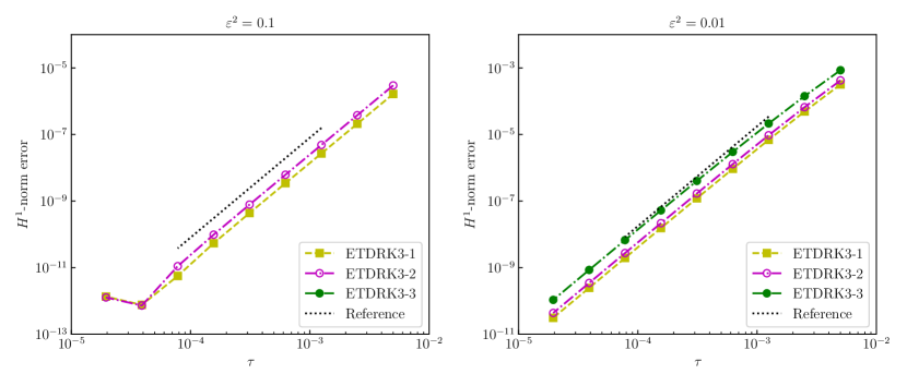
Figure 1: $H^{1}$ errors and convergence rates between the two temporally third-order ETDRK schemes.

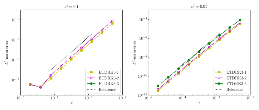
Figure 2: $L^{2}$ errors and convergence rates between the two temporally third-order ETDRK schemes.

5 Concluding remarks

In this paper, we systematically established the optimal convergence rate analysis for the two existing energy-stable third-order exponential time differencing Runge-Kutta (ETDRK3) schemes for the epitaxial thin film growth equation. We began by introducing the one-parameter ETDRK3 formulation and illustrating its corresponding Butcher-like tableau. Subsequently, we proved the discrete mass conservation law.

For the convergence analysis, we utilized eigenvalue bound estimates in Fourier space and applied the discrete $L^{2}$ inner product technique, combined with skillful operator estimates, to achieve the optimal fully discrete convergence result in the $\ell^{\infty}(0,T;H_{h}^{1})\cap\ell^{2}(0,T;H_{h}^{3})$ norm.

In numerical experiments, we compared the error performance of the three energy-stable schemes and found that the ETDRK3 scheme from [21] slightly outperformed the others from [22]. Notably, we relaxed one degree of freedom—referred to as the abscissa $c_{1}$ in the Butcher-like tableau—during the analysis, establishing a convergence framework applicable to energy-stable ETDRK3 schemes with varying abscissas. Finally, from the perspective of numerical experiments, our ongoing work will focus on determining the optimal abscissa $c_{1}$ (i.e., the one yielding the best accuracy) for such energy-stable ETDRK3 formulations (2.4).

Declarations

Funding The authors have not disclosed any funding.
Data Availbility Enquires about data availability should be directed to the authors.
Conflict of interest The authors have not disclosed any competing interests.

Appendix A Proof for Proposition 3.1

For simplicity of presentation, we only focus on the analysis for $j=1$; an extension to the case of $j=2$ or $3$ would be straightforward.

An application of $G_{\mathcal{N}}^{1,1}L_{\kappa}$ and $-\Delta_{\mathcal{N}}$ to the discrete Fourier expansion of $f$ turns out to be

$$\bigl{(}G_{\mathcal{N}}^{1,1}L_{\kappa}f\bigr{)}_{p,q}=\sum_{\ell,m=-K}^{K}\frac{1-\mathrm{e}^{-c_{1}\tau\Lambda_{\ell,m}}}{\tau\Lambda_{\ell,m}}\cdot\Lambda_{\ell,m}\hat{f}_{\ell,m}\mathrm{e}^{2\pi\mathrm{i}(\ell x_{p}+my_{q})/L};$$ (.1)

$$\bigl{(}-\Delta_{\mathcal{N}}f\bigr{)}_{p,q}=\sum_{\ell,m=-K}^{K}\lambda_{\ell,m}\hat{f}_{\ell,m}\mathrm{e}^{2\pi\mathrm{i}(\ell x_{p}+my_{q})/L},$$ (.2)

which in turn gives the discrete inner product as

$$\big{\langle}G_{\mathcal{N}}^{1,1}L_{\kappa}f,-\Delta_{\mathcal{N}}f\big{\rangle}=L^{2}\sum_{\ell,m=-K}^{K}\frac{1-\mathrm{e}^{-\tau\Lambda_{\ell,m}}}{\tau\Lambda_{\ell,m}}\cdot\Lambda_{\ell,m}\cdot\lambda_{\ell,m}^{2}\cdot|\hat{f}_{\ell,m}|^{2}.$$ (.3)

In the meantime, an application of Parseval equality to the discrete Fourier expansion of $G_{\mathcal{N}}^{1,1,(5)}f$ indicates that

$$\big{\|}G_{\mathcal{N}}^{1,1,(5)}f\big{\|}_{2}^{2}=L^{2}\sum_{\ell,m=-K}^{K}\frac{1-\mathrm{e}^{-c_{1}\tau\Lambda_{\ell,m}}}{\tau}\lambda_{\ell,m}\cdot|\hat{f}_{\ell,m}|^{2}.$$ (.4)

By making comparison between (.3) and (.4), the first equality in (3.25) has been proved. Moreover, we see that

$$\big{\|}G_{\mathcal{N}}^{1,1,(5)}f\big{\|}_{2}^{2} =L^{2}\sum_{\ell,m=-K}^{K}\frac{1-\mathrm{e}^{-c_{1}\tau\Lambda_{\ell,m}}}{\tau\Lambda_{\ell,m}}\Lambda_{\ell,m}\cdot\lambda_{\ell,m}\cdot|\hat{f}_{\ell,m}|^{2}$$ (.5)

$$=L^{2}\sum_{\ell,m=-K}^{K}\frac{1-\mathrm{e}^{-c_{1}\tau\Lambda_{\ell,m}}}{\tau\Lambda_{\ell,m}}\bigl{(}\varepsilon^{2}\lambda_{\ell,m}^{3}+\kappa\lambda_{\ell,m}^{2}\bigr{)}|\hat{f}_{\ell,m}|^{2}.$$

An application of Parseval equality to the discrete Fourier expansion of $G_{\mathcal{N}}^{1,1,(0)}\nabla_{\mathcal{N}}\Delta_{\mathcal{N}}f$ and $G_{\mathcal{N}}^{1,1,(0)}\Delta_{\mathcal{N}}f$ reveals that

$$\big{\|}G_{\mathcal{N}}^{1,1,(0)}\nabla_{\mathcal{N}}\Delta_{\mathcal{N}}f\big{\|}_{2}^{2}=L^{2}\sum_{\ell,m=-K}^{K}\frac{1-\mathrm{e}^{-c_{1}\tau\Lambda_{\ell,m}}}{\tau\Lambda_{\ell,m}}\cdot\lambda_{\ell,m}^{3}\cdot|\hat{f}_{\ell,m}|^{2},$$ (.6)

$$\big{\|}G_{\mathcal{N}}^{1,1,(0)}\Delta_{\mathcal{N}}f\big{\|}_{2}^{2}=L^{2}\sum_{\ell,m=-K}^{K}\frac{1-\mathrm{e}^{-c_{1}\tau\Lambda_{\ell,m}}}{\tau\Lambda_{\ell,m}}\cdot\lambda_{\ell,m}^{2}\cdot|\hat{f}_{\ell,m}|^{2}.$$ (.7)

By making a comparison between (.5), (.6), and (.7), the second inequality of (3.25) is proved.

Since the discrete Fourier expansion of $g-\varphi_{0}(c_{1}\tau L_{\kappa})f$ becomes

$$\bigl{(}g-\varphi_{0}(c_{1}\tau L_{\kappa})f\bigr{)}_{p,q}=\sum_{\ell,m=-K}^{K}\bigl{(}\hat{g}_{\ell,m}-\mathrm{e}^{-\tau L_{\kappa}}\hat{f}_{\ell,m}\bigr{)}\mathrm{e}^{2\pi\mathrm{i}(\ell x_{p}+my_{q})/L},$$

its discrete $H^{1}$ norm turns out to be

$$\big{\|}\nabla_{\mathcal{N}}\bigl{(}g-\varphi_{0}\bigl{(}c_{1}\tau L_{\kappa}\bigr{)}f\bigr{)}\big{\|}_{2}^{2}=L^{2}\sum_{\ell,m=-K}^{K}\lambda_{\ell,m}\cdot|\hat{g}_{\ell,m}-\mathrm{e}^{-c_{1}\tau L_{\kappa}}\hat{f}_{\ell,m}|^{2}.$$ (.8)

In addition, the discrete inner product of (.2) with $G_{\mathcal{N}}^{1,1}L_{\kappa}f$, in which the discrete Fourier expansion is given by (.1), yields

$$\big{\langle}G_{\mathcal{N}}^{1,1}L_{\kappa}f,-\Delta_{\mathcal{N}}\varphi_{0}(c_{1}\tau L_{\kappa})f\big{\rangle}=L^{2}\sum_{\ell,m=-K}^{K}\frac{1-\mathrm{e}^{-c_{1}\tau\Lambda_{\ell,m}}}{c_{1}\tau\Lambda_{\ell,m}}\cdot\Lambda_{\ell,m}\cdot\mathrm{e}^{-c_{1}\tau\Lambda_{\ell,m}}\cdot\lambda_{\ell,m}\cdot|\hat{f}_{\ell,m}|^{2}.$$ (.9)

Subsequently, a combination of the representation formulae (.9) and (.8) results in

$$c_{1}\tau\left\langle G_{\mathcal{N}}^{1,1}L_{\kappa}f,-\Delta_{\mathcal{N}}\varphi_{0}(c_{1}\tau L_{\kappa})f\right\rangle+\big{\|}\nabla_{\mathcal{N}}\bigl{(}g-\varphi_{0}(c_{1}\tau L_{\kappa})\bigr{)}\big{\|}_{2}^{2}$$

$$= L^{2}\sum_{\ell,m=-K}^{K}\Bigl{(}\bigl{(}1-\mathrm{e}^{-c_{1}\tau\Lambda_{\ell,m}}\bigr{)}\cdot\mathrm{e}^{-c_{1}\tau\Lambda_{\ell,m}}\cdot\lambda_{\ell,m}\cdot|\hat{f}_{\ell,m}|^{2}+\lambda_{\ell,m}\cdot|\hat{g}_{\ell,m}-\mathrm{e}^{-c_{1}\tau L_{\kappa}}\hat{f}_{\ell,m}|^{2}\Bigr{)}$$

$$= L^{2}\sum_{\ell,m=-K}^{K}\lambda_{\ell,m}\Bigl{(}\bigl{(}1-\mathrm{e}^{-c_{1}\tau\Lambda_{\ell,m}}\bigr{)}\cdot\mathrm{e}^{c_{1}\tau\Lambda_{\ell,m}}\cdot|\mathrm{e}^{-c_{1}\tau\Lambda_{\ell,m}}\hat{f}_{\ell,m}|^{2}+|\hat{g}_{\ell,m}-\mathrm{e}^{-c_{1}\tau L_{\kappa}}\hat{f}_{\ell,m}|^{2}\Bigr{)}$$

$$= L^{2}\sum_{\ell,m=-K}^{K}\lambda_{\ell,m}\bigl{(}1-\mathrm{e}^{-c_{1}\tau\Lambda_{\ell,m}}\bigr{)}\Bigl{(}\mathrm{e}^{c_{1}\tau\Lambda_{\ell,m}}\cdot|\mathrm{e}^{-c_{1}\tau\Lambda_{\ell,m}}\hat{f}_{\ell,m}|^{2}+\frac{1}{1-\mathrm{e}^{-\tau\Lambda_{\ell,m}}}|\hat{g}_{\ell,m}-\mathrm{e}^{-c_{1}\tau L_{\kappa}}\hat{f}_{\ell,m}|^{2}\Bigr{)}.$$

On the other hand, for each fixed mode frequency $(\ell,m)$, the following lower bound is observed:

$$\mathrm{e}^{c_{1}\tau\Lambda_{\ell,m}}a^{2}+\frac{1}{1-\mathrm{e}^{-c_{1}\tau\Lambda_{\ell,m}}}b^{2} =a^{2}+b^{2}+\bigl{(}\mathrm{e}^{c_{1}\tau\Lambda_{\ell,m}}-1\bigr{)}a^{2}+\Bigl{(}\frac{1}{1-\mathrm{e}^{-c_{1}\tau\Lambda_{\ell,m}}}-1\Bigr{)}b^{2}$$

$$\geq a^{2}+b^{2}+2ab=(a+b)^{2},$$

for any $a,~{}b\geq 0$, in which the Cauchy inequality has been applied in the second step. Then we obtain

$$\mathrm{e}^{c_{1}\tau\Lambda_{\ell,m}}\cdot|\mathrm{e}^{-c_{1}\tau\Lambda_{\ell,m}}\hat{f}_{\ell,m}|^{2}+\frac{1}{1-\mathrm{e}^{-\tau\Lambda_{\ell,m}}}|\hat{g}_{\ell,m}-\mathrm{e}^{-c_{1}\tau L_{\kappa}}\hat{f}_{\ell,m}|^{2}$$

$$\geq \Bigl{(}|\mathrm{e}^{-c_{1}\tau\Lambda_{\ell,m}}\hat{f}_{\ell,m}|+|\hat{g}_{\ell,m}-\mathrm{e}^{-c_{1}\tau L_{\kappa}}\hat{f}_{\ell,m}|\Bigr{)}^{2}\geq|\hat{g}_{\ell,m}|^{2},\mbox{ so that}$$

$$c_{1}\tau\left\langle G_{\mathcal{N}}^{1,1}L_{\kappa}f,-\Delta_{\mathcal{N}}\varphi_{0}(c_{1}\tau L_{\kappa})f\right\rangle+\big{\|}\nabla_{\mathcal{N}}\bigl{(}g-\varphi_{0}(c_{1}\tau L_{\kappa})\bigr{)}\big{\|}_{2}^{2}$$

$$\geq L^{2}\sum_{\ell,m=-K}^{K}\lambda_{\ell,m}\bigl{(}1-\mathrm{e}^{-\tau\Lambda_{\ell,m}}\bigr{)}|\hat{g}_{\ell,m}|^{2}.$$

In comparison with the representation formula for $c_{1}\tau\|G_{\mathcal{N}}^{1,1,(5)}g\|_{2}^{2}$:

$$c_{1}\tau\big{\|}G_{\mathcal{N}}^{1,1,(5)}g\big{\|}_{2}^{2} =c_{1}\tau L^{2}\sum_{\ell,m=-K}^{K}\frac{1-\mathrm{e}^{-c_{1}\tau\Lambda_{\ell,m}}}{c_{1}\tau\Lambda_{\ell,m}}\Lambda_{\ell,m}\cdot\lambda_{\ell,m}\cdot|\hat{g}_{\ell,m}|^{2}$$

$$=L^{2}\sum_{\ell,m=-K}^{K}\lambda_{\ell,m}\bigl{(}1-\mathrm{e}^{-c_{1}\tau\Lambda_{\ell,m}}\bigr{)}|\hat{g}_{\ell,m}|^{2}.$$

We conclude that (3.26) has been established, as well as (3.27) and (3.28).

Inequalities in (3.29) come from the discrete Fourier expansions (3.19)-(3.21) and (3.17)-(3.18), combined with the preliminary Calculus-style estimates in Lemma 2.5. This finishes the proof.

References

• [1] G. Ehrlich and Fo.G. Hudda, Atomic view of surface self-diffusion: tungsten on tungsten, Journal of Chemical Physics, 44 (1966), pp. 1039–1049.
• [2] R.L. Schwoebel, Step motion on crystal surfaces. II, Journal of Applied Physics, 40 (1969), pp. 614-618.
• [3] B. Li and J. Liu, Thin film epitaxy with or without slope selection, European Journal of Applied Mathematics, 14 (2003), pp. 713-743.
• [4] B. Li, High-order surface relaxation versus the Ehrlich–Schwoebel effect, Nonlinearity, 19 (2006), p. 2581.
• [5] W. Chen, S. Conde, C. Wang, X. Wang, and S. M. Wise, A linear energy stable scheme for a thin film model without slope selection, Journal of Scientific Computing, 52 (2012), pp. 546–562.
• [6] W. Chen, C. Wang, X. Wang, and S. M. Wise, A linear iteration algorithm for a second-order energy stable scheme for a thin film model without slope selection, Journal of Scientific Computing, 59 (2014), pp. 574–601.
• [7] Q. Cheng, J. Shen, and X. Yang, Highly efficient and accurate numerical schemes for the epitaxial thin film growth models by using the SAV approach, Journal of Scientific Computing, 78 (2019), pp. 1467–1487.
• [8] Y. Hao, Q. Huang, and C. Wang, A third order BDF energy stable linear scheme for the no-slope-selection thin film model, arXiv preprint arXiv:2011.01525 (2020).
• [9] W. Li, W. Chen, C. Wang, Y. Yan, and R. He, A second order energy stable linear scheme for a thin film model without slope selection, Journal of Scientific Computing, 76 (2018), pp. 1905–1937.
• [10] D. Li, Z. Qiao, and T. Tang, Characterizing the stabilization size for semi-implicit Fourier-spectral method to phase field equations, SIAM Journal on Numerical Analysis, 54 (2016), pp. 1653–1681.
• [11] Z. Qiao, Z.-Z. Sun, and Z. Zhang, Stability and convergence of second-order schemes for the nonlinear epitaxial growth model without slope selection, Mathematics of Computation, 84 (2015), pp. 653–674.
• [12] Z. Qiao, Z. Zhang, and T. Tang, An adaptive time-stepping strategy for the molecular beam epitaxy models, SIAM Journal on Scientific Computing, 33 (2011), pp. 1395–1414.
• [13] J. Shen, C. Wang, X. Wang, and S. M. Wise, Second-order convex splitting schemes for gradient flows with Ehrlich-Schwoebel type energy: application to thin film epitaxy, SIAM Journal on Numerical Analysis, 50 (2012), pp. 105–125.
• [14] C. Xu and T. Tang, Stability analysis of large time-stepping methods for epitaxial growth models, SIAM Journal on Numerical Analysis, 44 (2006), pp. 1759–1779.
• [15] D. J. Eyre,Unconditionally gradient stable time marching the Cahn-Hilliard equation, MRS online proceedings library (OPL), 529 (1998), p. 39.
• [16] L. Ju, X. Li, Z. Qiao, and H. Zhang, Energy stability and convergence of exponential time differencing schemes for the epitaxial growth model without slope selection, Mathematics of Computation, 87 (2018), pp. 1859–1885.
• [17] W. Chen, W. Li, Z. Luo, and C. Wang, A stabilized second order exponential time differencing multistep method for thin film growth model without slope selection, ESAIM: Mathematical Modelling and Numerical Analysis, 54 (2020), pp. 727–750.
• [18] W. Chen, W. Li, C. Wang, S. Wang, and X. Wang, Energy stable higher-order linear ETD multi-step methods for gradient flows: application to thin film epitaxy, Research in the Mathematical Sciences, 7 (2020), pp. 1–27.
• [19] Z. Fu and J. Yang, Energy-decreasing exponential time differencing Runge-Kutta methods for phase-field models, Journal of Scientific Computing, 454 (2022), p. 110943.
• [20] Y. Sun and Q. Zhou,Error Estimate of Exponential Time Differencing Runge-Kutta Scheme for the Epitaxial Growth Model Without Slope Selection, Journal of Scientific Computing, 93 (2022), p. 22.
• [21] W. Cao, H. Yang, and W. Chen,An Exponential Time Differencing Runge–Kutta Method ETDRK32 for Phase Field Models, Journal of Scientific Computing, 99 (2024), p. 6.
• [22] Z. Fu, J. Shen, and J. Yang,Higher-order energy-decreasing exponential time differencing Runge-Kutta methods for gradient flows, Science China Mathematics, (2024), pp. 1–20.
• [23] S. Gottlieb and C. Wang, Stability and convergence analysis of fully discrete Fourier collocation spectral method for 3-D viscous Burgers’ equation, Journal of Scientific Computing, 53 (2012), pp. 102–128.
• [24] W. E, Convergence of spectral methods for the Burgers’ equation, SIAM Journal on Numerical Analysis, 29 (1992), pp. 1520–1541.
• [25] W. E, Convergence of Fourier methods for Navier–Stokes equations, SIAM Journal on Numerical Analysis, 30 (1993), pp. 650–674.
• [26] M. Hochbruck and A. Ostermann, Explicit exponential Runge-Kutta methods for semilinear parabolic problems, SIAM Journal on Numerical Analysis, 43 (2005), pp. 1069–1090.
• [27] N. J. Higham, Functions of Matrices: Theory and Computation, SIAM, Philadelphia, PA, 2008.
• [28] M. Cui, Y. Niu, and Z. Xu, A Second-Order Exponential Time Differencing Multi-step Energy Stable Scheme for Swift–Hohenberg Equation with Quadratic-Cubic Nonlinear Term, Journal of Scientific Computing, 99 (2024).
• [29] S. Gottlieb, F. Tone, C. Wang, and X. Wang, Long time stability of a classical efficient scheme for two-dimensional Navier–Stokes equations, SIAM Journal on Numerical Analysis, 50 (2012), pp. 126–150.
• [30] S. Wise, C. Wang, and J. Lowengrub, An energy-stable and convergent finite-difference scheme for the phase field crystal equation, SIAM Journal on Numerical Analysis, 47 (2009), pp. 2269–2288.