One Node One Model: Featuring the Missing-Half for Graph Clustering

Abstract

Most existing graph clustering methods primarily focus on exploiting topological structure, often neglecting the “missing-half” node feature information, especially how these features can enhance clustering performance. This issue is further compounded by the challenges associated with high-dimensional features. Feature selection in graph clustering is particularly difficult because it requires simultaneously discovering clusters and identifying the relevant features for these clusters. To address this gap, we introduce a novel paradigm called “one node one model”, which builds an exclusive model for each node and defines the node label as a combination of predictions for node groups. Specifically, the proposed “Feature Personalized Graph Clustering (FPGC)” method identifies cluster-relevant features for each node using a squeeze-and-excitation block, integrating these features into each model to form the final representations. Additionally, the concept of feature cross is developed as a data augmentation technique to learn low-order feature interactions. Extensive experimental results demonstrate that FPGC outperforms state-of-the-art clustering methods. Moreover, the plug-and-play nature of our method provides a versatile solution to enhance GNN-based models from a feature perspective.

Introduction

As a fundamental task in graph data mining, attributed graph clustering aims to partition nodes into different clusters without labeled data. It is receiving increasing research attention due to the success of Graph Neural Networks (GNNs) (Welling and Kipf 2017; Li, Pan, and Kang 2024; Qian, Li, and Kang 2024). Typically, GNNs use many graph convolutional layers to learn node representations by aggregating neighbor node features into the node. In recent years, many graph clustering techniques have achieved promising performance (Pan and Kang 2023; Liu et al. 2023; Kang et al. 2024; Shen, Wang, and Kang 2024).

Most of these methods apply a self-supervised learning framework to fully explore the graph structure (Zhu et al. 2024; Yang et al. 2024), often neglecting the “missing-half” of node feature information, i.e., how node features can enhance clustering quality. Consequently, their performance heavily depends on the quality of the input graph. If the original graph is of poor quality, such as having many nodes from different classes connected together and missing important links, the representations learned through multilayer aggregation become nondiscrimination. This issue is known as representation collapse (Chen, Wang, and Li 2024).

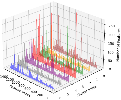
(a) Feature distribution of different clusters on Cora.

(b) DTW distance matrix with only cluster-relevant features on Cora.

Figure 1: Visualization of results on Cora. (a) is the feature distribution of different clusters, which shows that clusters are characterized by different features. (b) is the DTW distance matrix based on cluster-relevant features, which verify their distinctiveness. We can draw the conclusion that the cluster-relevant features contain valuable information about clusters.

For the attributed graph, the node feature and the topological structure should play an equal role in the unsupervised graph embedding and downstream clustering. We argue that a node’s personalized features should be crucial for identifying its cluster label. For example, the Cora dataset contains 2,708 papers, each described by a 1,433-dimensional binary feature indicating the presence of keywords. We visualize the feature distributions for each cluster in Fig. 1(a). It can be seen that each cluster exhibits its own dominant features, while other features may be irrelevant or less important. The cluster-relevant features are the collection of all personalized features. To distinguish between clusters, we consider features that are 20 times greater than the mean value in each cluster and apply the dynamic time warping (DTW) technique (Müller 2007) to each cluster. DTW is a similarity measure for sequences of different lengths, and we set the maximum distance to 5,000 for better visualization. From Fig. 1(b), we can see that there are significant differences in the cluster-relevant features. Thus, these personalized features are representative of different clusters.

Furthermore, most GNN-based methods capture only higher-order feature interactions and tend to overlook low-order interactions (Kim, Choi, and Kim 2024). The graph filtering process transforms input features into higher-level hidden representations. Recent studies on GNNs focus mainly on designing node aggregation mechanisms that emphasize various connection properties, such as local similarity (Welling and Kipf 2017), structural similarity (Donnat et al. 2018), and multi-hop connectivity (Li et al. 2022). However, the cross feature information is always ignored, despite its importance for model expressiveness (Feng et al. 2021). For example, by crossing a paper’s keywords in the Cora dataset, such as {$title=autonomous$ & $approach=Q-learning$ & $experiment=simulation$}, the model can achieve a better paper representation and produce more accurate clustering results (e.g., this paper is categorized under Reinforcement Learning). Until recently, most existing clustering models have struggled to capture such low-order feature interactions.

To address these shortcomings, we introduce “Feature Personalized Graph Clustering (FPGC)”. We propose a novel paradigm “one node one model” to learn a personalized model for each node, with a squeeze-and-excitation block selecting cluster-relevant features. A new data augmentation technique based on feature cross is developed to effectively capture low-order feature interactions. In summary, our contributions are as follows.

• Orthogonal to existing works, we tackle graph clustering from a feature perspective. By employing a squeeze-and-excitation block, we effectively select cluster-relevant features and propose the “one node one model” paradigm.

• We develop a novel data augmentation technique based on feature cross to capture low-order feature interactions.

• Extensive experiments on benchmark datasets demonstrate the superiority of our method. Notably, our approach can function as a plug-and-play tool for existing GNN-based models, rather than serving solely as a stand-alone method.

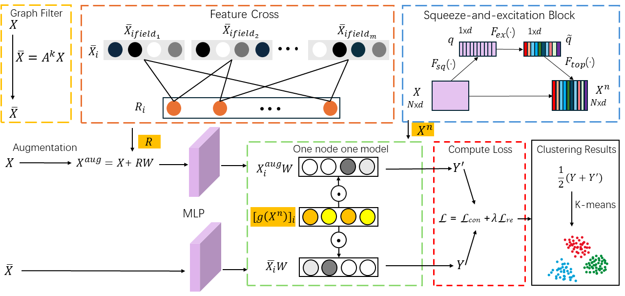
Figure 2: The pipeline of our FPGC. We preprocess the node features by stacked graph filters. Besides, we also input original features into the squeeze-and-excitation block to select the top $n$ significant features, based on which we learn a model for each node. Then, the contrastive framework encodes the smoothed node features and augmented features to achieve discriminative node representations.

Related work

Graph clustering can be roughly divided into three categories (Xie et al. 2024; Li et al. 2024). (1) Shallow methods. FGC (Kang et al. 2022) incorporates higher-order information into graph structure learning for clustering. MCGC (Pan and Kang 2021) uses simplified graph filtering rather than GNNs to obtain a smooth representation. (2) Contrastive methods. SCGC (Liu et al. 2023) simplifies network architecture and data augmentation. CCGC (Yang et al. 2023a) leverages high-confidence clustering information to improve sample quality. CONVERT (Yang et al. 2023b) uses a perturb-recover network and semantic loss for reliable data augmentation. (3) Autoencoder methods. SDCN (Bo et al. 2020) transfers learned representations from auto-encoders to GNN layers, employing data structure information. AGE (Cui et al. 2020) uses Laplacian smoothing filters and adaptive learning to improve node embeddings. DGCN (Pan and Kang 2023) uses an adaptive filter to capture important frequency information and reconstructs heterophilic and homophilic graphs to handle real-world graphs with different levels of homophily. DMGNC (Yang et al. 2024) uses a masked autoencoder for node feature reconstruction. However, their training is highly dependent on the input graph. Consequently, if the original graph is poor quality, the learned representation through multilayer aggregation becomes indiscriminate.

To improve the discriminability of representation, some recent methods learn node-specific information by considering the distinctness of each node (Zhu et al. 2024; Dai et al. 2021). NDLS (Zhang et al. 2021) assigns different filtering orders to each node based on its influence score. DyFSS (Zhu et al. 2024) learns multiple self-supervised learning task weights derived from a gating network considering the difference in the node neighbors. In an orthogonal way, in this paper, we improve the representation learning from a feature perspective. We perform an in-depth analysis of how the “one node one model” paradigm benefits clustering.

Methodology

Notation

Define the graph data as $\mathcal{G}=\{\mathcal{V},E,X\}$, where $\mathcal{V}$ represents a set of $N$ nodes and $e_{ij}\in E$ denotes the edge between node $i$ and node $j$. $X=\{X_{1},...,X_{N}\}^{\top}\in\mathbb{R}^{N\times d}$ is the feature matrix with $d$ dimensions, $X_{i}$ and $X_{.j}$ indicate the $i$-th row and the $j$-th column and of $X$, respectively. Adjacency matrix $\widetilde{A}\in\mathbb{R}^{N\times N}$ represents the graph structure. $D$ represents the degree matrix. The normalized adjacency matrix is $A=D^{-\frac{1}{2}}(\widetilde{A}+I)D^{-\frac{1}{2}}$, and the corresponding graph Laplacian is $L=I-A$.

The Pipeline of FPGC

The FPGC framework is shown in Fig. 2. Our design comprises two critical components. The first component concretizes “one node one model” with GNNs, with a squeeze-and-excitation block selecting cluster-relevant features. The second is the contrastive learning framework with a new data augmentation technique based on feature cross.

Squeeze-and-Excitation Block

Cluster-relevant features characterize the clusters. We design a squeeze-and-excitation block to select them.

Squeeze: The squeeze operation compresses the node features from $X\in\mathbb{R}^{N\times d}$ to $q\in\mathbb{R}^{1\times d}$. Specifically, it computes the summation of the features as follows:

$$q=F_{sq}\left(X\right)=\frac{1}{N}\sum_{i=1}^{N}X_{i},$$ (1)

where $q$ serves as a channel-wise statistic that captures global feature information.

Excitation: The excitation operation follows the squeeze step and aims to capture dependencies among all channels. It is a simple gating mechanism that uses the sigmoid function $\sigma(\cdot)$ to activate the squeezed feature map, enabling the learning of nonlinear connections between channels. Firstly, the dimension is reduced using a multi-layer perceptron (MLP) $W_{1}$. Next, a ReLU function $\delta(\cdot)$ and another MLP $W_{2}$ are used to increase the dimensionality, returning it to the original dimension $d$. Finally, the sigmoid function is applied. The process is summarized as follows:

$$\tilde{q} =F_{ex}\left(q\right)=\sigma\left(W_{2}\delta\left(W_{1}q\right)\right).$$ (2)

Selection: The outcome of the excitation operation is considered to be the significance of each feature. Then, we define the function $F_{top}$ to select top $n$ important features according to $\tilde{q}$. This operation is defined as follows:

$$X^{n}=F_{top}\left(\tilde{q}X\right),$$ (3)

where $X^{n}\in\mathbb{R}^{N\times n}$ is the node feature matrix containing the top $n$ significant features.

One Node One Model

Ideally, an exclusive model should be constructed for each individual node, which is the core of our method:

$$Y_{i}=f^{(i)}(X_{i}),$$ (4)

where $Y$ and $f$ are the predicted label and the model. In this paradigm, personalization is fully maintained in the models. Unfortunately, the enormous number of nodes makes this scheme unfeasible. One possible solution is establishing several individual models for each type of cluster (the nodes in a group share personalized features). Each node can be considered as a combination of different clusters. For example, in a social network, a person is a member of both a mathematics group and several sports interest groups. Due to the diversity of these different communities, he may exhibit different characteristics when interacting with members from various communities. Specifically, the information about the mathematics group may be related to his professional research, while the information about sports clubs may be associated with his hobbies. As a result, we can decompose the output for a specific node as a combination of predictions for clusters:

$$Y_{i}=\sum_{j=1}^{M}w_{j}f^{(j)}(X_{i}),$$ (5)

where $j$ denotes the model index and there are $M$ models. For an unsupervised task, learning $w_{j}$ directly is difficult. Instead, we generate $w_{j}$ from personalized features: $w_{j}=\left[g(X^{n})\right]_{j}$, where $g(X^{n})=\sigma\left(W_{3}X^{n}\right)$. In other words, we use personalized features to identify clusters. A higher value of a personalized feature corresponds to a higher weight. $W_{3}$ represents an MLP.

For simplicity, we only consider SGC (Wu et al. 2019) as our basic model, i.e. $f^{(j)}(X_{i})=A_{i}^{k}XW^{j}$, where $A^{k}$ denotes the stacked $k$-layer graph filter. Other GNNs can also be the base models. For instance, DAGNN (Liu, Gao, and Ji 2020) has $f^{(j)}(X_{i})=\sum\limits_{t=0}^{k}s_{t}A_{i}^{t}XW^{j}$, where $s_{t}$ is the learnable weight; APPNP (Gasteiger, Bojchevski, and Günnemann 2018) has $f^{(j)}(X_{i})=\operatorname{softmax}\left(\eta(\boldsymbol{I}-(1-\eta)A)^{-1}_{i}X\right)W^{j}$, where $\eta$ is the a hyper-parameter. For convenience, we define $\bar{X}=A^{k}X=\{\bar{X}_{1},...,\bar{X}_{N}\}^{\top}$. Note that $\bar{X}_{j}\in\mathbb{R}^{d}$ and $W^{j}\in\mathbb{R}^{d\times d_{out}}$, where $d_{out}$ is the output dimension. We have:

$$Y_{i}=\sum_{j=1}^{M}\left[g\left(X^{n}\right)\right]_{j}\bar{X}_{i}W^{j}.$$ (6)

The $u$-th entry of $Y_{i}$ is given by:

$$Y_{iu}=\sum_{j=1}^{M}\sum_{v=1}^{d}\left[g\left(X^{n}\right)\right]_{j}W_{uv}^{j}\bar{X}_{iv},$$ (7)

which introduces a complexity of $M$ times. Thus far, we still need to design $M$ individual models to identify clusters, which is computationally demanding. Fortunately, we have enough free parameters to simplify the process. Here we present a simple yet effective way. We set $M=d_{out}$, which gives $Y_{i}=\sum\limits_{j=1}^{d_{out}}\sum\limits_{v=1}^{d_{in}}\left(\left[g\left(X^{n}\right)\right]_{j}W_{uv}^{j}\bar{X}_{iv}\right)$. Then we let $W_{uv}^{j}=\left\{\begin{array}[]{l}W_{uv},j=u\\ 0,j\neq u\end{array}\right.$, which yields:

$$Y_{iu} =\left[g\left(X^{n}\right)\right]_{u}\sum_{v=1}^{d}W_{uv}\bar{X}_{iv}$$ (8)

$$=\left[g\left(X^{n}\right)\right]_{u}\bar{X}_{i}W_{.u},$$

or equivalently,

$$Y=g\left(X^{n}\right)\odot\bar{X}W,$$ (9)

where $\odot$ denotes the Hadamard product. Consequently, learning a model for each node is achieved through element-wise multiplication, which is computationally efficient.

$\mathbb{Flexibility}$: Note that the above approach is a generic method to customize existing techniques rather than a stand-alone way. It can be seamlessly incorporated with many SOTA GNN models to enhance performance.

Theoretical Analysis

Most theoretical analysis in the GNN area focuses on graph structures (Mao et al. 2024). In this section, we establish a theoretical analysis from the feature perspective. Without loss of generality, we consider the case with two clusters, $c_{1}$ and $c_{2}$. Assume the original node features follow the Gaussian distribution: $X_{i}\sim N\left(\boldsymbol{\mu}_{1},\mathbf{I}\right)\text{ for }i\in c_{1}\text{ and }X_{i}\sim N\left(\boldsymbol{\mu}_{2},\mathbf{I}\right)\text{ for }i\in c_{2}$ ($\boldsymbol{\mu}_{1}\boldsymbol{\mu}_{2}\geq$ 0). We define the filtered feature as $\bar{X}=D^{-1}\widetilde{A}X$. We define $f_{i}$ and $f_{j}$ as models for $X_{i}$ and $X_{j}$, respectively, focusing on the personalized features in sets $T_{i}$ and $T_{j}$, while other irrelevant features are ignored. We then present the following theorem:

Theorem 1.

Assuming the distribution of filtered features $\bar{X}$ shares the same variance $\sigma\mathbf{I}$ and the cluster has a balance distribution $\mathbf{P}\left(Y=c_{1}\right)=\mathbf{P}\left(Y=c_{2}\right)$. The upper bound of $\left|\mathbf{P}\left(Y_{i}=c_{1}\mid f_{i}(\bar{X}_{i})\right)-\mathbf{P}\left(Y_{j}=c_{1}\mid f_{j}(\bar{X}_{j})\right)\right|$ is decreasing with respect to $\sum_{u\in{T_{i}\cap T_{j}}}\bar{X}_{iu}\bar{X}_{ju}$.

Note that the assumptions are not strictly necessary but are used to simplify the proof in the Appendix. Theorem 1 indicates that if two nodes share more cluster-relevant features, they are more likely to be classified into one cluster, and vice versa.

Contrastive Clustering

Feature Cross Augmentation

Although graph filtering can smooth the features between node neighborhoods, it only captures high-order feature interactions and suffers from overlooking low-order feature interaction (Feng et al. 2021). Feature cross can provide valuable information for downstream tasks. For example, features like {$title$ & $approach$ & $experiment$} can provide additional information about the paper’s category. Features that collectively represent $title$ can be viewed as a field, like $title=\left\{0,1,0\right\}$. To this end, we randomly divide the filtered features into $m$ fields:

$$\bar{X}=\{\bar{X}_{field_{1}},\bar{X}_{field_{2}},...,\bar{X}_{field_{m}}\}.$$ (10)

Then, every node has $m$ fields, i.e., $\bar{X_{i}}=\{\bar{X}_{ifield_{1}},\bar{X}_{ifield_{2}},...,\bar{X}_{ifield_{m}}\}$. We use $\bar{X}$ instead of $X$ because $\bar{X}$ has more information. The feature cross is defined as:

$$R_{i}=\left\{\bar{X}_{ifield_{z}}\bar{X}^{\top}_{ifield_{j}}\mid 1\leq z<j\leq m\right\},$$ (11)

We input the original features $X$ as a view for contrastive learning. It’s well known that matrix factorization techniques can capture the low-order interaction (Guo et al. 2017). Thus, we propose to perform data augmentation as follows:

$$X^{aug}=X+RW,$$ (12)

where $W$ is an MLP to adjust the dimension. Unlike previous methods, Eq.(12) has two advantages. First, instead of using typical graph enhancements such as feature masking or edge perturbation, our method generates augmented views from filtered features. This maintains the semantics of the augmented view. Second, other learnable augmentations design complex losses to remain close to the initial features. Eq.(12) is based on the feature cross, which can provide rich semantic information. The complexity of the feature cross is $O(Nm^{2})$, which is linear to $N$. The results can be stored and accessed after a one-time computation.

Similarly to Eq.(9), the second view is finally formulated as:

$$Y^{\prime}=g\left(X^{n}\right)\odot X^{aug}W.$$ (13)

Note that the same node in two different views shares the same model.

Loss Function

For two views $Y$ and $Y^{\prime}$, we treat the same node in different views as positive samples and all other nodes as negative samples. The pairwise loss is defined as follows:

$$\ell\left(Y_{i},Y^{\prime}_{i}\right)=-\log\frac{e^{\operatorname{sim}\left(Y_{i},Y^{\prime}_{i}\right)}}{\sum_{j=1}^{N}e^{\operatorname{sim}\left(Y_{i},Y^{\prime}_{j}\right)}+\sum_{j=1}^{N}e^{\operatorname{sim}\left(Y_{i},Y_{j}\right)}},$$ (14)

$$\mathcal{L}_{con}=\frac{1}{2N}\sum_{i=1}^{N}\left[\ell\left(Y_{i},Y^{\prime}_{i}\right)+\ell\left(Y^{\prime}_{i},Y_{i}\right)\right],$$

where $\operatorname{sim}$ is the cosine similarity. Besides, the reconstruction loss can be calculated as follows:

$$\mathcal{L}_{re}=\frac{1}{N^{2}}\left\|Y^{\prime}Y^{\top}-A\right\|_{F}.$$ (15)

Finally, the total loss is formulated as:

$$\mathcal{L}=\mathcal{L}_{re}+\lambda\mathcal{L}_{con},$$ (16)

where $\lambda>0$ is a trade-off parameter. The clustering results are obtained by performing K-means on $\frac{1}{2}(Y+Y^{\prime})$. The detailed learning process of FPGC is illustrated in the Appendix.

Experiments

Datasets

We select seven graph clustering benchmark datasets, which are: Cora (Yang, Cohen, and Salakhudinov 2016), CiteSeer (Yang, Cohen, and Salakhudinov 2016), Pubmed (Yang, Cohen, and Salakhudinov 2016), Amazon Photo (AMAP) (Liu et al. 2022), USA Air-Traffic (UAT) (Mrabah et al. 2022), Europe Air-Traffic (EAT) (Mrabah et al. 2022), and Brazil Air Traffic (BAT) (Mrabah et al. 2022). We also add two large-scale graph datasets, the image relationship network Flickr (Zeng et al. 2020) and the social network Twitch-Gamers (Rozemberczki and Sarkar 2021). To see the relevance between graph structure and downstream task, we also report the Aggregation Class Distance (ACD) (Shen, He, and Kang 2024).The statistics information is summarized in Table 1. We can see that these datasets are inherently low-quality.

Table 1: Statistics information of datasets.

Graph datasets		Nodes	Dims.	Edges	Clusters	ACD
	Cora	2708	1433	5429	7	0.52
	Citeseer	3327	3703	4732	6	0.36
	Pubmed	19717	500	44327	3	0.36
	UAT	1190	239	13599	4	0.35
	AMAP	7650	745	119081	8	0.28
	EAT	399	203	5994	4	0.25
	BAT	1190	239	13599	4	0.46
	Flickr	89250	500	899756	7	0.02
	Twitch-Gamers	168114	7	67997557	2	0.09

Comparison Methods

To demonstrate the superiority of FPGC, we compare it to several recent baselines. These methods can be roughly divided into three kinds: 1) traditional GNN-based methods: SSGC (Zhu and Koniusz 2021). 2) shallow methods: MCGC (Pan and Kang 2021), FGC (Kang et al. 2022), and CGC (Xie et al. 2023). 3) contrastive learning-based methods: MVGRL (Hassani and Khasahmadi 2020), SDCN (Bo et al. 2020), DFCN (Tu et al. 2021), SCGC (Liu et al. 2023), CCGC (Yang et al. 2023a), and CONVERT (Yang et al. 2023b). 4) Advanced autoencoder-based methods: AGE (Cui et al. 2020), DGCN (Pan and Kang 2023), DMGNC (Yang et al. 2024), and DyFSS (Zhu et al. 2024).

Experimental Setting

To ensure fairness, all experimental settings follow the DGCN (Pan and Kang 2023), which performs a grid search to find the best results. Our network is trained with the Adam optimizer for 400 epochs until convergence. Three MLPs consist of a single embedding layer, with 100 dimensions on Flickr and Twitch-Gamers, and 500 dimensions on other datasets. The learning rate is set to 1e-2 on BAT/EAT/UAT/Twitch-Gamers, 1e-3 on Cora/Citeseer/Pumbed/Flickr, and 1e-4 on AMAP. The graph aggregating layers $k$ is searched in {2,3,4,5}. The number of fields $m$ is set according to the density of features, i.e., denser features should have smaller values to cross fewer times, the number of important features $n$ is set according to the number of features, i.e., more features should have larger values, the trade-off parameter $\lambda$ is tuned in {0.001, 0.1, 1, 100}. Thus, $\left\{k,m,n,\lambda\right\}$ are set to $\left\{3,60,100,1\right\}$ on Cora, $\left\{4,50,50,0.1\right\}$ on Citeseer, $\left\{5,10,10,0.001\right\}$ on Pubmed, $\left\{5,20,10,100\right\}$ on UAT, $\left\{2,10,10,0.001\right\}$ on AMAP, $\left\{4,10,10,0.001\right\}$ on EAT, $\left\{5,20,20,1\right\}$ on BAT, $\left\{4,10,100,1\right\}$ on Flickr and $\left\{2,2,4,1\right\}$ on Twitch-Gamers. We evaluate clustering performance with two widely used metrics: ACC and NMI. All experiments are conducted on the same machine with the Intel(R) Core(TM) i9-12900k CPU, two GeForce GTX 3090 GPUs, and 128GB RAM .

Table 2: Clustering Results. The best performance is marked in red. “-” indicates the original paper does not have this result and the provided code can’t produce the result.

Methods	Cora		Citeseer		Pubmed		UAT		AMAP		EAT		BAT
	ACC	NMI	ACC	NMI	ACC	NMI	ACC	NMI	ACC	NMI	ACC	NMI	ACC	NMI
DFCN	36.33	19.36	69.50	43.90	-	-	33.61	26.49	76.88	69.21	32.56	8.27	35.56	8.25
SSGC	69.60	54.71	69.11	42.87	-	-	36.74	8.04	60.23	60.37	32.41	4.65	36.74	8.04
MVGRL	70.47	55.57	68.66	43.66	-	-	44.16	21.53	45.19	36.89	32.88	11.72	37.56	29.33
SDCN	60.24	50.04	65.96	38.71	65.78	29.47	52.25	21.61	53.44	44.85	39.07	8.83	53.05	25.74
AGE	73.50	57.58	70.39	44.92	-	-	52.37	23.64	75.98	-	47.26	23.74	56.68	36.04
MCGC	42.85	24.11	64.76	39.11	66.95	32.45	41.93	16.64	71.64	61.54	32.58	7.04	38.93	23.11
FGC	72.90	56.12	69.01	44.02	70.01	31.56	53.03	27.06	71.04	-	36.84	10.07	47.33	18.90
CONVERT	74.07	55.57	68.43	41.62	68.78	29.72	57.36	28.75	77.19	62.70	58.35	33.36	78.02	53.54
SCGC	73.88	56.10	71.02	45.25	67.73	28.65	56.58	28.07	77.48	67.67	57.94	33.91	77.97	52.91
CGC	75.15	56.90	69.31	43.61	67.43	33.07	49.58	17.49	73.02	63.26	44.32	30.25	53.44	26.97
CCGC	73.88	56.45	69.84	44.33	68.06	30.92	56.34	28.15	77.25	67.44	57.19	33.85	75.04	50.23
DGCN	72.19	56.04	71.27	44.13	-	-	52.27	23.54	76.07	66.13	51.27	31.98	70.15	49.52
DMGNC	73.12	54.80	71.27	44.40	70.46	34.21	-	-	-	-	-	-	-	-
DyFSS	72.19	55.49	70.18	44.80	68.05	26.87	51.43	25.52	76.86	67.78	43.36	21.23	77.25	51.33
FPGC	79.19	59.55	72.59	46.36	71.03	34.57	58.07	30.64	78.44	69.40	58.90	34.24	79.38	55.57

Results Analysis

The results are illustrated in Table LABEL:resultall. We find that FPGC achieves dominant performance in all cases. For example, on the Cora dataset, FPGC surpasses the runner-up by 4.04% and 2.65% in terms of ACC and NMI. Traditional GNN-based methods have poor performance compared to other methods, which dig for more structure information or use contrastive learning to implicitly capture the supervision information. Note that SCGC, CCGC, and CONVERT are the most recent contrastive methods that design new augmentations. Our method constantly exceeds advanced GNN-based methods with adaptive filters, which indicates the significance of fully exploring feature information.

DMGNC and DyFSS are the latest methods that explicitly consider feature information. DMGNC’s performance does not show clear advantages compared to other baselines on Cora and Citeseer. Though applying a node-wise feature fusion strategy, DyFSS also performs poorly. For example, our method’s ACC and NMI are 7.00% and 4.06% higher on Cora, and 15.54% and 13.01% higher on EAT, respectively. This is because they perform general embedding without exploiting the relationship between features and clusters.

Parameter Analysis

To assess the impact of parameters, we evaluate the clustering accuracy of FPGC across them on Cora and EAT. First, we test the performance with different $m$ and $n$. As shown in Fig. 3, Cora is less sensitive to these two parameters than EAT. In addition, Cora prefers a large $m$ while EAT opts for a small $m$, this is consistent with the density (proportion of non-zero values) of $\bar{X}$: 38.69% on Cora and 50.25% on EAT. Too large $m$ will degrade the performance since excessive augmentation could deteriorate the original information. Cora prefers a large $n$ while EAT opts for a small one, which is reasonable since the attribute dimension of Cora is much larger.

Secondly, the impact of $k$ and $\lambda$ is shown in Fig. 4. FPGC can perform in effect for a wide range of $\lambda$. A small $k$ is enough to achieve a decent result.

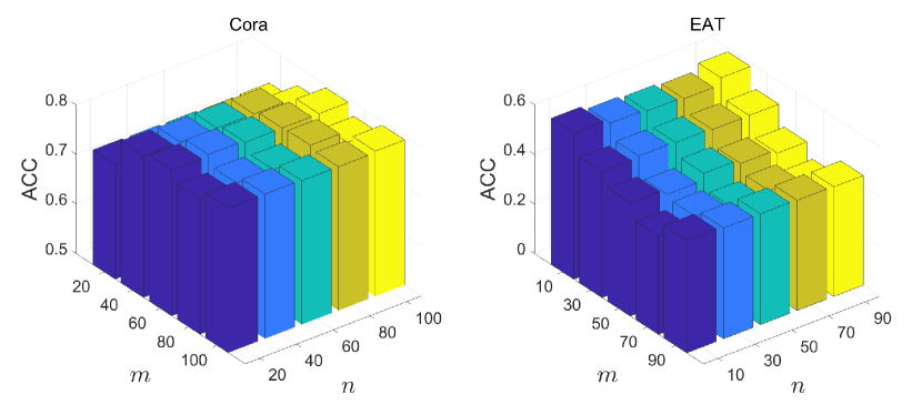
Figure 3: Parameter analysis of $m$ and $n$ on Cora and EAT.

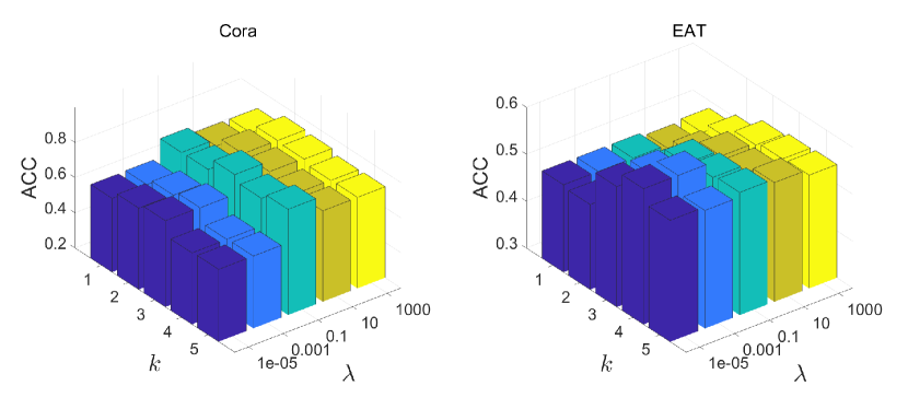
Figure 4: Parameter analysis of $k$ and $\lambda$ on Cora and EAT.

Results on Large-scale Data

To evaluate the scalability of FPGC, we conduct the experiments on large graph datasets Flickr and Twitch-Gamers, which have 89250 and 168114 nodes, respectively. Note that many methods fail to run on these datasets, such as DGCN. We set the batch size to 1000 for all methods. We select three recent baselines to see their performance and the total training time. Fig. 5 shows the results. FPGC continues to outperform all comparison approaches. The required training time of FPGC is notably lower than that of the CGC and DyFSS and exhibits a marginal advantage over CCGC. This is because the feature-personalized step involves only matrix multiplication, while graph filtering and feature crossing can be pre-computed and stored. The result not only highlights the effectiveness of FPGC but also underscores its scalability and efficiency in handling large-scale datasets.

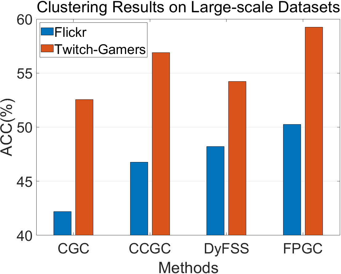
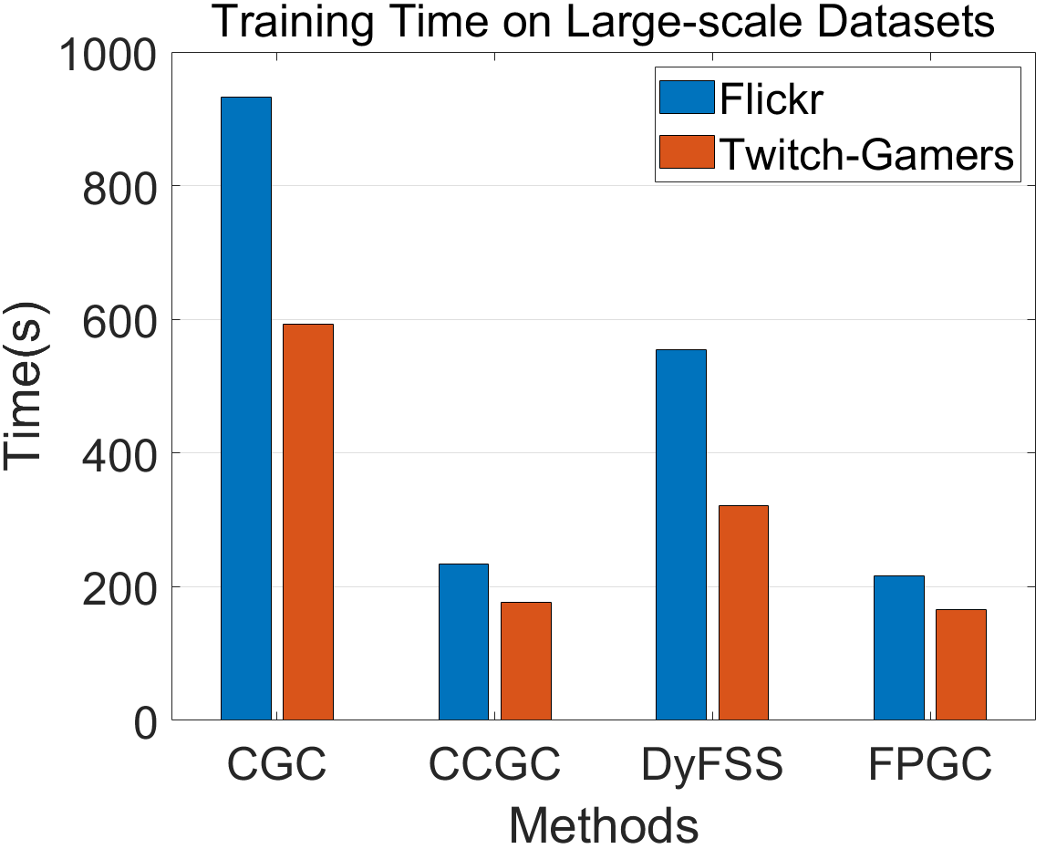
Figure 5: Clustering results and running time on Flickr and Twitch-Gamers.

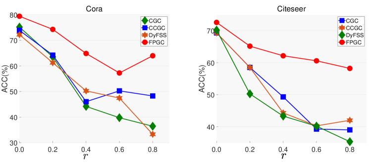
Figure 6: Results of robustness test on Cora (left) and Citeseer (right).

Table 3: Results of ablation study. The best performance is marked in red and the runner-up is marked in bold.

Methods	FPGC $w/o$ $aug$		FPGC $w$ $aug$		FPGC $w/o$ $g()$		FPGC $w$ DAGNN		FPGC
	ACC	NMI	ACC	NMI	ACC	NMI	ACC	NMI	ACC	NMI
Cora	75.95	58.98	76.42	57.52	78.52	58.72	78.27	59.02	79.19	59.55
Citeseer	71.04	44.90	71.33	44.65	70.23	44.34	72.10	46.02	72.59	46.36
Pubmed	66.98	28.47	67.76	29.42	71.20	34.96	72.05	35.26	71.03	34.57
UAT	57.25	29.06	57.61	29.69	57.13	29.86	58.24	30.72	58.07	30.64
AMAP	77.45	68.32	78.01	68.96	76.88	66.74	79.52	70.22	78.44	69.40
EAT	57.82	33.32	58.05	33.96	57.25	33.19	59.28	34.71	58.90	34.24
BAT	78.12	53.81	78.23	53.96	77.23	52.19	79.03	55.02	79.38	55.57

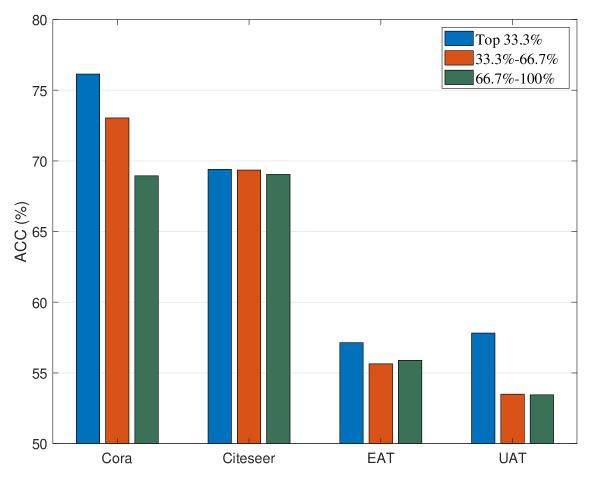
Figure 7: The results on different important features.

Robustness Analysis

To demonstrate the significance of the feature, we examine the situation in which the graph structure is of poor quality. Specifically, we add edges to the graphs and remove the same number of original edges from them at random (Fu, Zhao, and Bian 2022). We define $r=\frac{\text{\#random edges}}{\text{\#all edges}}$ as the random edge rate. With $r$ = {0.2, 0.4, 0.6, 0.8}, we report the ACC of CGC, CCGC, DyFSS, and FPGC in Cora and Citeseer. From Fig. 6, it can be seen that the PFGC achieves the best performance in all cases. Especially when the perturbation rate is extremely high, our method shows a more stable tendency than other clustering methods. The performance of other methods changes dramatically, indicating that they rely highly on the graph structure. Thus, our method is robust to the graph structure noise.

Ablation Study

To assess the impact of feature cross, we test the clustering performance after removing it, marking it as “FPGC $w/o$ $aug$”. The results are shown in Table 3. It is clear that feature cross does improve the clustering performance. In addition, we replace feature cross with classical graph augmentation strategies, including drop edges (Liu et al. 2024), add edges (Xia et al. 2022), graph diffusion (Hassani and Khasahmadi 2020), and mask feature (Yu et al. 2022). We set the change rate to 20% according to the suggestions of the original paper. The best performance among these four methods is marked as “FPGC $w$ $aug$”. Our method can still beat them, thus feature cross can provide more rich information.

To see the influence of feature selection, we test the performance without $g(X^{n})$ and mark it as “FPGC $w/o$ $g()$”. We can see the performance degradation in most cases in Table 3. Thus learning a model for each node can successfully keep each node’s personality. FPGC does not achieve better performance on Pubmed. This may be because Pubmed has a large node size but only has 3 clusters, which means that it is difficult to select the cluster-relevant features in this case. We also test the performance with DAGNN (Liu, Gao, and Ji 2020) as the base model and mark this method as “FPGC $w$ DAGNN”. It can be seen that it achieves the best performance in 4 out of 7 cases in Table 3. Thus, our proposed “one node one model” paradigm is promising with other SOTA GNNs.

To verify that the proposed squeeze-and-excitation block can select essential features, we categorize them into three intervals: features with the top 33.3% (highest) $\tilde{q}$, features from 33.3% to 66.7%, and the remaining 66.7% to 100%. We use these indexes to select features for $X^{n}$ and test their performance, respectively. From Fig. 7, we can see that when selecting the most important features (top 33.3%), we achieve the best results in all cases. This indicates that features with high value in $\tilde{q}$ are vital. Therefore, our proposed squeeze-and-excitation block can successfully assign high weights to essential features, which is beneficial for downstream task.

Conclusion

In this paper, we introduce the “one node one model” paradigm, which addresses the limitations of existing graph clustering methods by emphasizing missing-half feature information. By incorporating a squeeze-and-excitation block to select cluster-relevant features, our method effectively enhances the discriminative power of the learned representations. The proposed feature cross data augmentation further enriches the information available for contrastive learning. Our theoretical analysis and experimental results demonstrate that our method significantly improves clustering performance.

See pages 1 of Appendix.pdf See pages 2 of Appendix.pdf See pages 3 of Appendix.pdf

References

- Bo et al. (2020) Bo, D.; Wang, X.; Shi, C.; Zhu, M.; Lu, E.; and Cui, P. 2020. Structural deep clustering network. In Proceedings of The Web Conference 2020, 1400–1410.
- Chen, Wang, and Li (2024) Chen, M.; Wang, B.; and Li, X. 2024. Deep Contrastive Graph Learning with Clustering-Oriented Guidance. In Proceedings of the AAAI Conference on Artificial Intelligence, volume 38, 11364–11372.
- Cui et al. (2020) Cui, G.; Zhou, J.; Yang, C.; and Liu, Z. 2020. Adaptive graph encoder for attributed graph embedding. In Proceedings of the 26th ACM SIGKDD International Conference on Knowledge Discovery & Data Mining, 976–985.
- Dai et al. (2021) Dai, S.; Lin, H.; Zhao, Z.; Lin, J.; Wu, H.; Wang, Z.; Yang, S.; and Liu, J. 2021. POSO: personalized cold start modules for large-scale recommender systems. arXiv preprint arXiv:2108.04690.
- Donnat et al. (2018) Donnat, C.; Zitnik, M.; Hallac, D.; and Leskovec, J. 2018. Learning structural node embeddings via diffusion wavelets. In Proceedings of the 24th ACM SIGKDD international conference on knowledge discovery & data mining, 1320–1329.
- Feng et al. (2021) Feng, F.; He, X.; Zhang, H.; and Chua, T.-S. 2021. Cross-GCN: Enhancing Graph Convolutional Network with k-Order Feature Interactions. IEEE Transactions on Knowledge and Data Engineering, 35(1): 225–236.
- Fu, Zhao, and Bian (2022) Fu, G.; Zhao, P.; and Bian, Y. 2022. -Laplacian Based Graph Neural Networks. In International Conference on Machine Learning, 6878–6917. PMLR.
- Gasteiger, Bojchevski, and Günnemann (2018) Gasteiger, J.; Bojchevski, A.; and Günnemann, S. 2018. Predict then Propagate: Graph Neural Networks meet Personalized PageRank. In International Conference on Learning Representations.
- Guo et al. (2017) Guo, H.; Tang, R.; Ye, Y.; Li, Z.; and He, X. 2017. DeepFM: a factorization-machine based neural network for CTR prediction. In IJCAI, 1725–1731.
- Hassani and Khasahmadi (2020) Hassani, K.; and Khasahmadi, A. H. 2020. Contrastive multi-view representation learning on graphs. In International Conference on Machine Learning, 4116–4126. PMLR.
- Kang et al. (2022) Kang, Z.; Liu, Z.; Pan, S.; and Tian, L. 2022. Fine-grained Attributed Graph Clustering. In Proceedings of the 2022 SIAM International Conference on Data Mining (SDM), 370–378. SIAM.
- Kang et al. (2024) Kang, Z.; Xie, X.; Li, B.; and Pan, E. 2024. CDC: A Simple Framework for Complex Data Clustering. IEEE Transactions on Neural Networks and Learning Systems.
- Kim, Choi, and Kim (2024) Kim, M.; Choi, H.-S.; and Kim, J. 2024. Explicit Feature Interaction-Aware Graph Neural Network. IEEE Access, 12: 15438–15446.
- Li, Pan, and Kang (2024) Li, B.; Pan, E.; and Kang, Z. 2024. Pc-conv: Unifying homophily and heterophily with two-fold filtering. In Proceedings of the AAAI Conference on Artificial Intelligence, volume 38, 13437–13445.
- Li et al. (2024) Li, B.; Xie, X.; Lei, H.; Fang, R.; and Kang, Z. 2024. Simplified PCNet with Robustness. arXiv preprint arXiv:2403.03676.
- Li et al. (2022) Li, X.; Zhu, R.; Cheng, Y.; Shan, C.; Luo, S.; Li, D.; and Qian, W. 2022. Finding global homophily in graph neural networks when meeting heterophily. In International Conference on Machine Learning, 13242–13256. PMLR.
- Liu, Gao, and Ji (2020) Liu, M.; Gao, H.; and Ji, S. 2020. Towards deeper graph neural networks. In Proceedings of the 26th ACM SIGKDD international conference on knowledge discovery & data mining, 338–348.
- Liu et al. (2022) Liu, Y.; Tu, W.; Zhou, S.; Liu, X.; Song, L.; Yang, X.; and Zhu, E. 2022. Deep graph clustering via dual correlation reduction. In Proceedings of the AAAI Conference on Artificial Intelligence, volume 36, 7603–7611.
- Liu et al. (2023) Liu, Y.; Yang, X.; Zhou, S.; Liu, X.; Wang, S.; Liang, K.; Tu, W.; and Li, L. 2023. Simple contrastive graph clustering. IEEE Transactions on Neural Networks and Learning Systems, 35(10): 13789–13800.
- Liu et al. (2024) Liu, Y.; Zhou, S.; Yang, X.; Liu, X.; Tu, W.; Li, L.; Xu, X.; and Sun, F. 2024. Improved Dual Correlation Reduction Network With Affinity Recovery. IEEE Transactions on Neural Networks and Learning Systems.
- Mao et al. (2024) Mao, H.; Chen, Z.; Jin, W.; Han, H.; Ma, Y.; Zhao, T.; Shah, N.; and Tang, J. 2024. Demystifying structural disparity in graph neural networks: Can one size fit all? Advances in neural information processing systems, 36.
- Mrabah et al. (2022) Mrabah, N.; Bouguessa, M.; Touati, M. F.; and Ksantini, R. 2022. Rethinking graph auto-encoder models for attributed graph clustering. IEEE Transactions on Knowledge and Data Engineering, 35(9): 9037–9053.
- Müller (2007) Müller, M. 2007. Dynamic time warping. Information retrieval for music and motion, 69–84.
- Pan and Kang (2021) Pan, E.; and Kang, Z. 2021. Multi-view contrastive graph clustering. Advances in neural information processing systems, 34: 2148–2159.
- Pan and Kang (2023) Pan, E.; and Kang, Z. 2023. Beyond homophily: Reconstructing structure for graph-agnostic clustering. In International Conference on Machine Learning, 26868–26877. PMLR.
- Qian, Li, and Kang (2024) Qian, X.; Li, B.; and Kang, Z. 2024. Upper Bounding Barlow Twins: A Novel Filter for Multi-Relational Clustering. In Proceedings of the AAAI Conference on Artificial Intelligence, volume 38, 14660–14668.
- Rozemberczki and Sarkar (2021) Rozemberczki, B.; and Sarkar, R. 2021. Twitch gamers: a dataset for evaluating proximity preserving and structural role-based node embeddings. arXiv preprint arXiv:2101.03091.
- Shen, He, and Kang (2024) Shen, Z.; He, H.; and Kang, Z. 2024. Balanced Multi-Relational Graph Clustering. In Proceedings of the 32nd ACM International Conference on Multimedia (MM’24).
- Shen, Wang, and Kang (2024) Shen, Z.; Wang, S.; and Kang, Z. 2024. Beyond Redundancy: Information-aware Unsupervised Multiplex Graph Structure Learning. Advances in Neural Information Processing Systems.
- Tu et al. (2021) Tu, W.; Zhou, S.; Liu, X.; Guo, X.; Cai, Z.; Zhu, E.; and Cheng, J. 2021. Deep fusion clustering network. In Proceedings of the AAAI Conference on Artificial Intelligence, volume 35, 9978–9987.
- Welling and Kipf (2017) Welling, M.; and Kipf, T. N. 2017. Semi-supervised classification with graph convolutional networks. In J. International Conference on Learning Representations.
- Wu et al. (2019) Wu, F.; Souza, A.; Zhang, T.; Fifty, C.; Yu, T.; and Weinberger, K. 2019. Simplifying graph convolutional networks. In International conference on machine learning, 6861–6871. PMLR.
- Xia et al. (2022) Xia, W.; Wang, Q.; Gao, Q.; Yang, M.; and Gao, X. 2022. Self-consistent contrastive attributed graph clustering with pseudo-label prompt. IEEE Transactions on Multimedia, 25: 6665–6677.
- Xie et al. (2023) Xie, X.; Chen, W.; Kang, Z.; and Peng, C. 2023. Contrastive graph clustering with adaptive filter. Expert Systems with Applications, 219: 119645.
- Xie et al. (2024) Xie, X.; Pan, E.; Kang, Z.; Chen, W.; and Li, B. 2024. Provable Filter for Real-world Graph Clustering. arXiv preprint arXiv:2403.03666.
- Yang et al. (2024) Yang, J.; Cai, J.; Zhong, L.; Pi, Y.; and Wang, S. 2024. Deep Masked Graph Node Clustering. IEEE Transactions on Computational Social Systems, 11(6): 7257–7270.
- Yang et al. (2023a) Yang, X.; Liu, Y.; Zhou, S.; Wang, S.; Tu, W.; Zheng, Q.; Liu, X.; Fang, L.; and Zhu, E. 2023a. Cluster-guided contrastive graph clustering network. In Proceedings of the AAAI conference on artificial intelligence, volume 37, 10834–10842.
- Yang et al. (2023b) Yang, X.; Tan, C.; Liu, Y.; Liang, K.; Wang, S.; Zhou, S.; Xia, J.; Li, S. Z.; Liu, X.; and Zhu, E. 2023b. Convert: Contrastive graph clustering with reliable augmentation. In Proceedings of the 31st ACM International Conference on Multimedia, 319–327.
- Yang, Cohen, and Salakhudinov (2016) Yang, Z.; Cohen, W.; and Salakhudinov, R. 2016. Revisiting semi-supervised learning with graph embeddings. In International Conference on Machine Learning, 40–48. PMLR.
- Yu et al. (2022) Yu, L.; Pei, S.; Ding, L.; Zhou, J.; Li, L.; Zhang, C.; and Zhang, X. 2022. Sail: Self-augmented graph contrastive learning. In Proceedings of the AAAI Conference on Artificial Intelligence, volume 36, 8927–8935.
- Zeng et al. (2020) Zeng, H.; Zhou, H.; Srivastava, A.; Kannan, R.; and Prasanna, V. 2020. GraphSAINT: Graph Sampling Based Inductive Learning Method. In International Conference on Learning Representations.
- Zhang et al. (2021) Zhang, W.; Yang, M.; Sheng, Z.; Li, Y.; Ouyang, W.; Tao, Y.; Yang, Z.; and Cui, B. 2021. Node dependent local smoothing for scalable graph learning. Advances in Neural Information Processing Systems, 34: 20321–20332.
- Zhu and Koniusz (2021) Zhu, H.; and Koniusz, P. 2021. Simple Spectral Graph Convolution. In 9th International Conference on Learning Representations, ICLR 2021.
- Zhu et al. (2024) Zhu, P.; Wang, Q.; Wang, Y.; Li, J.; and Hu, Q. 2024. Every Node is Different: Dynamically Fusing Self-Supervised Tasks for Attributed Graph Clustering. In Proceedings of the AAAI Conference on Artificial Intelligence, volume 38, 17184–17192.