waveOrder: generalist framework for label-agnostic computational microscopy

Abstract

Correlative computational microscopy is accelerating the mapping of dynamic biological systems by integrating morphological and molecular measurements across spatial scales, from organelles to entire organisms. Visualization, measurement, and prediction of interactions among the components of biological systems can be accelerated by generalist computational imaging frameworks that relax the trade-offs imposed by multiplex dynamic imaging. This work reports a generalist framework for wave optical imaging of the architectural order (waveOrder) among biomolecules for encoding and decoding multiple specimen properties from a minimal set of acquired channels, with or without fluorescent labels. waveOrder expresses material properties in terms of elegant physically motivated basis vectors directly interpretable as phase, absorption, birefringence, diattenuation, and fluorophore density; and it expresses image data in terms of directly measurable Stokes parameters. We report a corresponding multi-channel reconstruction algorithm to recover specimen properties in multiple contrast modes. With this framework, we implement multiple 3D computational microscopy methods, including quantitative phase imaging, quantitative label-free imaging with phase and polarization, and fluorescence deconvolution imaging, across scales ranging from organelles to whole zebrafish. These advances are available via an extensible open-source computational imaging library, waveOrder, and a napari plugin, recOrder.

1 Introduction

Biological functions emerge from the interaction of many components that span length scales, i.e., biomolecules, organelles, cells, tissues, and organs. Correlative imaging of these components’ physical and molecular properties is a growing area of microscopy. Computational imaging methods that optically encode multiple physical and molecular properties and decode them computationally are particularly promising as they relax the trade-offs between spatial resolution, temporal resolution, number of channels, field of view, and sample health that constrain multiplex dynamic imaging.

Correlative label-free and fluorescence imaging "fills the vacuum" of observing a few fluorescent molecules in complex biological environments. These approaches enable measurement of conserved physical properties of cellular compartments [1] and enable dynamic high-throughput imaging for mapping responses of multiple organelles to complex perturbations [2]. Such correlative datasets have enabled the development of neural networks that virtually stain molecular labels from label-free contrast modes [3, 4, 5], further improving the ability to analyze interactions among organelles and cells. Light-sheet fluorescence microscopy has long been used to measure the dynamic interactions of cells [6] and organelles [7, 2]. At scales larger than organelles, recent methods for spatial mapping of gene expression [8], protein distribution [9], and gene perturbations [10] use multi-channel imaging systems that encode multiple molecular species in the imaging data. At the finer scale of biomolecular complexes, cryo-CLEM (correlative light and electron microscopy) reveals the structural basis of the biomolecular function [11, 12].

The microscopy methods used by the above technologies can be modeled via linear image formation models, even though they rely on diverse light-matter interactions. The visualization, measurement, and analysis of specimen properties in these biological studies can be improved by developing a computational imaging framework that reconstructs specimen properties from the acquired multi-channel imaging data. This paper describes a computational imaging framework that addresses this need.

2 Background and prior work

Many works describe microscopic image formation for individual contrast modes including fluorescence contrast [13, 14], phase and absorption contrast [15, 16], and polarization-resolved birefringence contrast [17, 18]. Recently, multiple papers have developed computational imaging methods for integrative measurements of specimen properties, but with models specific to label-free contrast [3, 19, 20, 21, 22] or fluorescence contrast [23, 24]. The waveOrder framework unifies and extends these models to multi-contrast and multi-channel imaging systems that include scalar and polarization-resolved imaging with or without fluorescence labels.

The most general image formation models account for statistical fluctuations in the electric field of light, i.e., coherence, and how the coherence is modulated due to propagation or interaction with matter. Modeling coherence requires bilinear functions (functions whose output depends on pairs of points in the imaging path) and propagation of second-order statistics [25, 15, 26, 27, 28, 29]. We start with this approach before restricting our attention to imaging problems that can be modeled with linear functions. Specifically, we consider spatially incoherent fluorescence samples and label-free imaging systems with a spatially incoherent source.

Several existing frameworks provide some, but not all, of the features of waveOrder. Deconvolution libraries typically focus on fluorescence deconvolution [30, 31], limiting their value in multi-channel correlative settings. Differentiable microscopy libraries [32, 33] flexibly model a wide variety of imaging systems to enable new designs and reconstructions, but they don’t often provide generalist inverse algorithms applicable to diverse contrast mechanisms. waveOrder prioritizes linear reconstruction models for the most widely used computational microscopy contrast methods, facilitating broad applications.

We also find that many reconstruction implementations are not used broadly for biological research because they are not reproducible or easy to access. waveOrder is an open-source and actively developed project that attempts to maximize the usability and impact of linear computational imaging methods by unifying and maintaining the most valuable reconstruction techniques in biological microscopy. waveOrder leverages PyTorch for cross-platform, high-performance analysis of large datasets and integration with learned computer vision models.

In our view, this paper makes the following contributions

• a simulation and reconstruction framework that can be applied to linear microscopy contrast modes, including fluorescence, phase, absorption, birefringence, and diattenuation;

• clear links between material properties, their light-matter interactions, and the mathematical operators that represent them;

• a demonstration of reconstructions of simulated phantoms, physical phantoms, and biological samples across length scales; and

• demonstrates reconstructions across the scales of organelles, cells, organs, and organisms using a PyTorch-based library.

3 waveOrder framework

We start by describing a framework for reconstructing material properties from microscopic imaging data. By representing material properties and data as vectors, we describe our reconstructions as the solution to an optimization problem. Using broadly applicable assumptions of linearity, shift invariance, and weak scattering, we describe all contrasts as the result of banks of point spread functions. We describe the physics behind the major contrast mechanisms and compute their transfer functions from illumination, scattering, and detection models. Throughout, we use carefully chosen basis functions to enable the physical interpretation of light and material properties. We describe all notation as we introduce it, and we collect all symbols in Supplement 1.

3.1 Objects and data as vectors, imaging as an operator

We represent a biological sample as a series of volumetric maps of material properties, shown schematically in Figure 1a, i. For example, a cell might be approximately described by two fluorophore density maps, $f_{1}(\mathbf{r}_{o})$ and $f_{2}(\mathbf{r}_{o})$ where $\mathbf{r}_{o}$ is a 3D object position vector, one map for each of two different fluorophores that label biological structures of interest, and a density map $\rho(\mathbf{r}_{o})$. Three maps are unlikely to describe the sample completely, so we generalize and collect any number of volumetric maps into a single vector

$$\mathbf{f}=[\mathbf{f}_{1},\mathbf{f}_{2},\mathbf{f}_{3},\ldots]^{T}=[f_{1}(\mathbf{r}_{o}),f_{2}(\mathbf{r}_{o}),\rho(\mathbf{r}_{o}),\ldots]^{T},$$ (1)

which represents all of the properties of our sample.

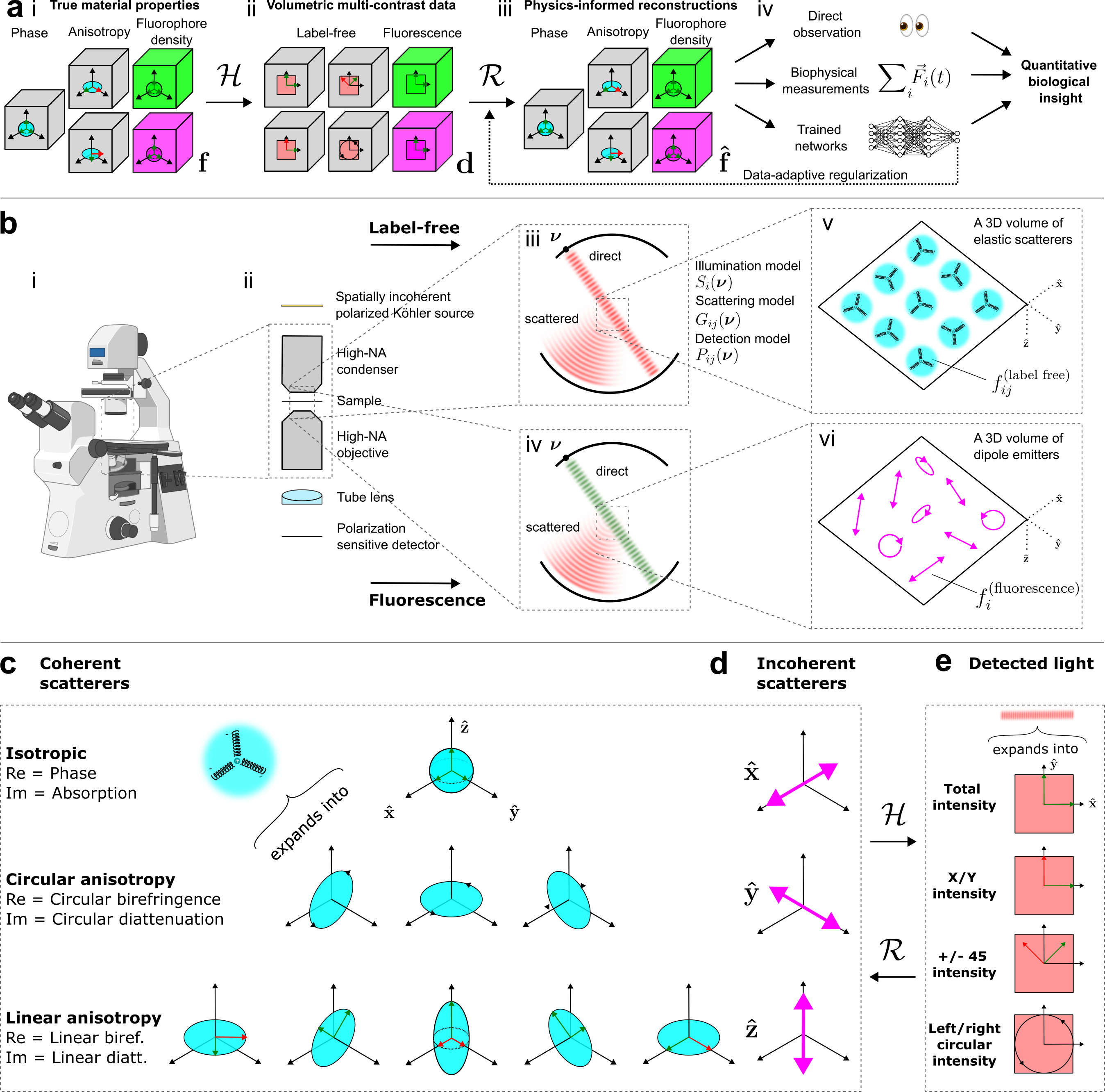
Figure 1: A framework for volumetric microscopy of phase, absorption, birefringence, diattenuation, fluorescence density, and fluorescence orientation. (a) Microscopes encode (i) true material properties into (ii) multi-contrast multi-channel volumetric datasets by changing spectral and polarization illumination and detection filters. Physics-informed models of the encoding process, $\mathcal{H}$, lead to physics-informed reconstruction operators, $\mathcal{R}$, that enable (iii) reconstructions of underlying material properties. (iv) We find that physics-informed reconstructions are useful for improving performance on downstream observation, biophysical, and learned tasks. (b) We model the encoding process of an (i) off-the-shelf inverted microscope stand outfitted with (ii) an incoherent source, variable spectral and polarization filters, and a polarization-sensitive detector. Two classes of contrast are available: label-free contrast where (iii) direct fields scatter coherently from the sample and direct-scatter interference generates contrast, and (iv) fluorescence contrast where direct fields that excite inelastic-scattering fluorophores are filtered so that scatter-scatter interference generates contrast. We model coherent scatterers as (v) a volume of scattering potential tensors that model the relationship between incident electric fields and induced dipoles moments. We model inelastic fluorescence scatterers as (vi) a volume of dipole emission moments. Both coherent and incoherent dipoles can be linear, circular, and elliptical, though fluorescent dipoles used in biological microscopy are primarily linear. (c) Expanding the scattering potential tensor onto spherical harmonic tensors enables interpretation in terms of phase, absorption, birefringence, and diattenuation. (d) Expanding dipole emitters into Cartesian components with complex coefficients enables interpretation of single emitters’ orientations. (e) Expanding measurable data into Stokes parameters enables modeling of all possible polarization measurements. See also Video 1.

When we image our sample in a microscope, we arrange for the material properties to be encoded into a list of volumetric datasets, each called a channel, shown schematically in Figure 1a, ii. For example, we might use a fluorescence light path to encode fluorophore density maps into two channels, $d_{1}(\mathbf{r}_{d})$ and $d_{2}(\mathbf{r}_{d})$ where $\mathbf{r}_{d}$ is a 3D detector position vector, then we can change to a transmission light path to encode the density $\rho(\mathbf{r}_{o})$ into the third channel $d_{3}(\mathbf{r}_{d})$. Similar to our object properties, we collect any number of channels into a single vector

$$\mathbf{d}=[\mathbf{d}_{1},\mathbf{d}_{2},\mathbf{d}_{3},\ldots]^{T}=[d_{1}(\mathbf{r}_{d}),d_{2}(\mathbf{r}_{d}),d_{3}(\mathbf{r}_{d}),\ldots]^{T},$$ (2)

which represents all of the data we collect from our sample.

We can represent the imaging process with a single forward operator $\mathcal{H}$ that encodes the material properties $\mathbf{f}$ into measured volumetric datasets $\mathbf{d}$

$$\mathbf{d}=\mathcal{H}\mathbf{f}+\mathbf{b},$$ (3)

where $\mathbf{b}$ is a spatially uniform background in each channel. Note that $\mathcal{H}$ might encode multiple material properties into a single channel. For example, the material properties of phase and anisotropy can be jointly encoded into several label-free data channels.

3.2 Reconstructing object properties

We would like to recover as much as we can about the object’s material properties $\mathbf{f}$ from the measured data $\mathbf{d}$, but we are faced with a major problem—the forward operator $\mathcal{H}$ is never invertible. There are always object properties that are invisible to the imaging system, and one way to find invisible properties is to make the properties smaller than the resolution limit of the imaging system. For example, if we have a visible-light microscopy dataset $\mathbf{d}$ there are an infinite number of molecular-scale configurations that could result in the same dataset, so we have no hope of choosing a single $\mathbf{f}$ as the true measured properties.

We need to choose a single set of material properties from among the infinite possible solutions that agree with the data—a reconstruction problem. Our strategy is to choose the material properties that minimize a scalar objective function $Q(\mathbf{f},\mathbf{d})$

$$\mathbf{\hat{f}}=\mathcal{R}\mathbf{d}=\operatorname*{argmin}_{\mathbf{f}}Q(\mathbf{f},\mathbf{d}),$$ (4)

where the $\operatorname*{argmin}$ notation means that we choose as our solution $\mathbf{\hat{f}}$ the $\mathbf{f}$ that minimizes the value of $Q(\mathbf{f},\mathbf{d})$. One choice is the least-squares objective $Q^{\text{(ls)}}(\mathbf{f},\mathbf{d})=\left\|\mathbf{d}-\mathbf{b}-\mathcal{H}\mathbf{f}\right\|_{2}^{2},$ but this solution tends to amplify noise. A better choice is a Tikhonov-regularized least-squares objective

$$Q_{\eta}^{\text{(tls)}}(\mathbf{f},\mathbf{d})=\left\|\mathbf{d}-\mathbf{b}-\mathcal{H}\mathbf{f}\right\|_{2}^{2}-\eta\|\mathbf{f}\|_{2}^{2},$$ (5)

which adds a regularization parameter $\eta$ that suppresses the size of the solution $\mathbf{f}$, an example of a prior that penalizes large solutions. Many other objective functions are possible, including those that include physics-informed and learned priors.

After choosing an objective function, the minimization problem needs to be solved, an often challenging task. Fortunately, if $\mathcal{H}$ is linear then the Tikhonov-regularized least-squares objective can be minimized in a single step described in Supplement 5, generating efficient noise-tolerant estimates of material properties, Figure 1a, iii.

As illustrated in Figure 1a, iv, physics-informed reconstruction operators prepare raw microscopy data for improved direct visual inspection, improved biophysical estimates [1], and improved performance on tasks performed by trained networks [5]. Therefore, the next sections develop physically interpretable models of light-matter interactions for diverse contrast modes.

3.3 Contrast modes

We model the image formation process of an off-the-shelf inverted microscope stand (Figure 1b, i–ii) outfitted with a spatially incoherent Köhler source with variable polarization filters, variable spectral filters, a high-NA condenser and objective, and an imaging path that includes a polarization-sensitive detector.

All contrast is formed by illuminating the sample with electric fields that scatter from the sample then interfere on the detector. If we consider only single scattering events, the first Born approximation, then we can rewrite Equation 3 as

$$\mathbf{d}=\left|\mathcal{S}\mathbf{f}+\mathbf{e}^{\text{(d)}}\right|^{2},$$ (6)

where $\mathcal{S}$ is a scattering operator that models the scattered fields that reach the detector and $\mathbf{e}^{(d)}$ models the unscattered direct fields that reach the detector. Expanding the square reveals four terms

$$\mathbf{d}=|\mathcal{S}|^{2}|\mathbf{f}|^{2}+\mathbf{e}^{\dagger\text{(d)}}\mathcal{S}\mathbf{f}+\mathbf{f}^{\dagger}\mathcal{S}^{\dagger}\mathbf{e}^{(\text{d})}+|\mathbf{e}^{\text{(d)}}|^{2},$$ (7)

that we refer to as the scatter-scatter, scatter-direct, direct-scatter, and direct-direct terms, respectively, and $\dagger$ denotes conjugate transpose.

We consider two classes of contrast. Label-free contrast (Figure 1b, iii) is generated by illuminating the sample with light that interacts with the sample coherently—that is, scattered fields have the same wavelength and a fixed phase relationship with the illuminating fields. When a plane wave encounters a coherent scatterer, the oscillating electric field accelerates bound electrons in the scatterer, and these accelerated charges generate spherical scattered fields. The direct and scattered fields interfere and generate contrast via the scatter-direct and direct-scatter terms. The direct-direct term creates a uniform background, and for weakly scattering samples the scatter-scatter term is small and ignorable. Therefore, label-free contrast is generated by the direct-scatter and scatter-direct terms on top of a direct-direct background. Finally, each point on the source emits incoherently, so we can treat each source point individually and find the complete contrast pattern by summing over the source.

Fluorescence contrast (Figure 1b, iv) is generated by illuminating fluorescent scatterers and imaging their scattered light. Fluorescent scatterers are incoherent, so the scattered fields have a random phase at a longer wavelength than the illuminating fields. Therefore, the scatter-direct and direct-scatter terms do not generate contrast, so the only way to measure sample-dependent contrast is via the small scatter-scatter term. Fortunately, the direct and scattered fields are at different wavelengths, so the direct fields can be filtered with minimal bleedthrough. Therefore, fluorescence contrast is generated by the scatter-scatter term with a direct-direct bleedthrough background. Finally, fluorescent scatterers emit incoherently, so we can find the complete contrast pattern by summing over the sample.

Both label-free and fluorescence contrast modes can generate additional contrast from anisotropic samples. Label-free samples can be anisotropic if the scatterer’s bound electrons accelerate anisotropically. We illustrate a label-free anisotropic sample schematically as an electron bound to its nucleus by springs of varying spring constant (Figure 1b, v). When polarized light is incident on an anisotropic sample, it accelerates the bound electrons in linear, circular, or elliptical dipoles, which emit anisotropic polarized light in patterns that encode the orientation of the induced electron motion and the underlying anisotropy of the scatterer. Therefore, information about the sample’s label-free anisotropy is encoded in the polarization and intensity pattern of the detected light. Similarly, fluorescent scatterers emit along linear, circular, or elliptical dipoles (Figure 1b, vi), though linear dipoles are most common among the fluorophores used in biological microscopy.

3.4 Physically interpretable basis functions

When we illuminate a label-free sample, the 3D induced dipole moment is the product of the incident field and a 3 $\times$ 3 matrix called the permittivity tensor [29, 21]. By convention, we change to a unitless quantity and subtract the isotropic background (Supplement 6) to arrive at a complete set of label-free sample properties—the complex-valued 3 $\times$ 3 matrix called the scattering potential tensor, $f^{(\text{lf})}_{ij}$. Each entry of the scattering potential tensor can be interpreted directly (e.g. the complex-valued $f^{(\text{lf})}_{xz}$ is the relative magnitude and phase of the $x$ component of the dipole induced by a $z$-oriented field), but this interpretation can be challenging to understand physically. To improve physical interpretability, we expand the scattering potential tensor onto the spherical harmonic tensors, a set of nine 3 $\times$ 3 matrices whose complex-valued expansion coefficients can be directly interpreted in terms of phase, absorption, birefringence, and diattenuation. We schematize each of these spherical harmonic tensors in Figure 1c by drawing each tensor’s eigenvalues and eigenvectors, and we describe the spherical harmonic tensor basis in detail in Supplement 6.

In a fluorescent sample, the 3D emission dipole moment can be represented by a three-component vector $f^{(\text{fl})}_{i}$ (Figure 1d) with real-valued coefficients for purely linear dipoles and complex-valued coefficients for arbitrary dipoles. Contrast arises from the scatter-scatter term, so our measurements are proportional to the squares of the dipole components $|f^{(\text{fl})}_{i}|^{2}$.

For dynamic ensembles of fluorescent emitters, the measurements are proportional to the second-moment matrix $\langle f^{(\text{fl})}_{i}f^{*(\text{fl})}_{j}\rangle$ [13, 34, 23]. Similar to the scattering potential tensor, we can expand the second-moment matrix onto the spherical harmonic tensors, but here we interpret the coefficients in terms of orientation distribution functions [14, 24].

Finally, we express our data in terms of the Stokes parameters, a set of four real-valued parameters that are physically interpretable as the intensities measured behind various polarizing filters. The Stokes parameters can also be interpreted as the coefficients of the electric field’s second-moment matrix expanded onto the Pauli matrices (Figure 1e, Supplement 7).

3.5 Linear contrast-separable shift-invariant imaging systems

Under approximations that are applicable to a wide range of microscopes (details in Section 5 and Supplement 8), we can model our imaging system by splitting our material properties, data channels, and forward model into independent groups called contrast modes, e.g. one label-free mode and several fluorescence modes. Each of these contrast modes is approximately linear across object properties, and each property-to-channel mapping is approximately spatially linear and shift invariant. Therefore, we can express our imaging model as

$$d^{(m)}_{c}(\mathbf{r}_{d})=\sum_{p}\int d\mathbf{r}_{o}\,h^{(m)}_{cp}(\mathbf{r}_{d}-\mathbf{r}_{o})f^{(m)}_{p}(\mathbf{r}_{o})+b_{c}^{(m)},$$ (8)

where $m$ indexes contrast $m$odes, $p$ indexes material $p$roperties, $c$ indexes data $c$hannels, and $h^{(m)}_{cp}$ is a bank of point spread functions that model the entire multi-contrast multi-channel imaging system. We can reexpress this relationship in the Fourier domain as

$$D^{(m)}_{c}(\boldsymbol{\nu})=\sum_{p}H^{(m)}_{cp}(\boldsymbol{\nu})F^{(m)}_{p}(\boldsymbol{\nu})+b_{c}^{(m)}\delta(\boldsymbol{\nu}).$$ (9)

where $\boldsymbol{\nu}$ is a 3D spatial frequency coordinate, capital letters denote 3D Fourier transforms, and $H^{(m)}_{cp}(\boldsymbol{\nu})$ is a bank of transfer functions that model the transmission of spatial frequency components through the imaging system. We inspect the properties of these transfer functions next.

3.6 Summary of transfer functions

The waveOrder framework calculates all transfer functions from three core submodels:

1. an illumination model—the vector source pupil $S_{i}(\boldsymbol{\nu})$,

2. a scattering model—the Green’s tensor spectrum $G_{ij}(\boldsymbol{\nu})$,

3. a detection model—the tensor detection pupil $P_{ij}(\boldsymbol{\nu})$.

All three submodels are expressed as complex-valued spherical shell functions with radius $1/\lambda$ in the frequency domain, where $\lambda$ is the wavelength in the imaging media.

The Green’s tensor spectrum is particularly important for modeling anisotropic contrast. Linear dipole moments emit polarized light in a doughnut-shaped intensity pattern (Figure 2a), and the Green’s tensor spectrum (Figure 2b) efficiently models all dipole emitters (coherent or incoherent; linear, circular, or elliptical dipoles in any orientation) with a single function.

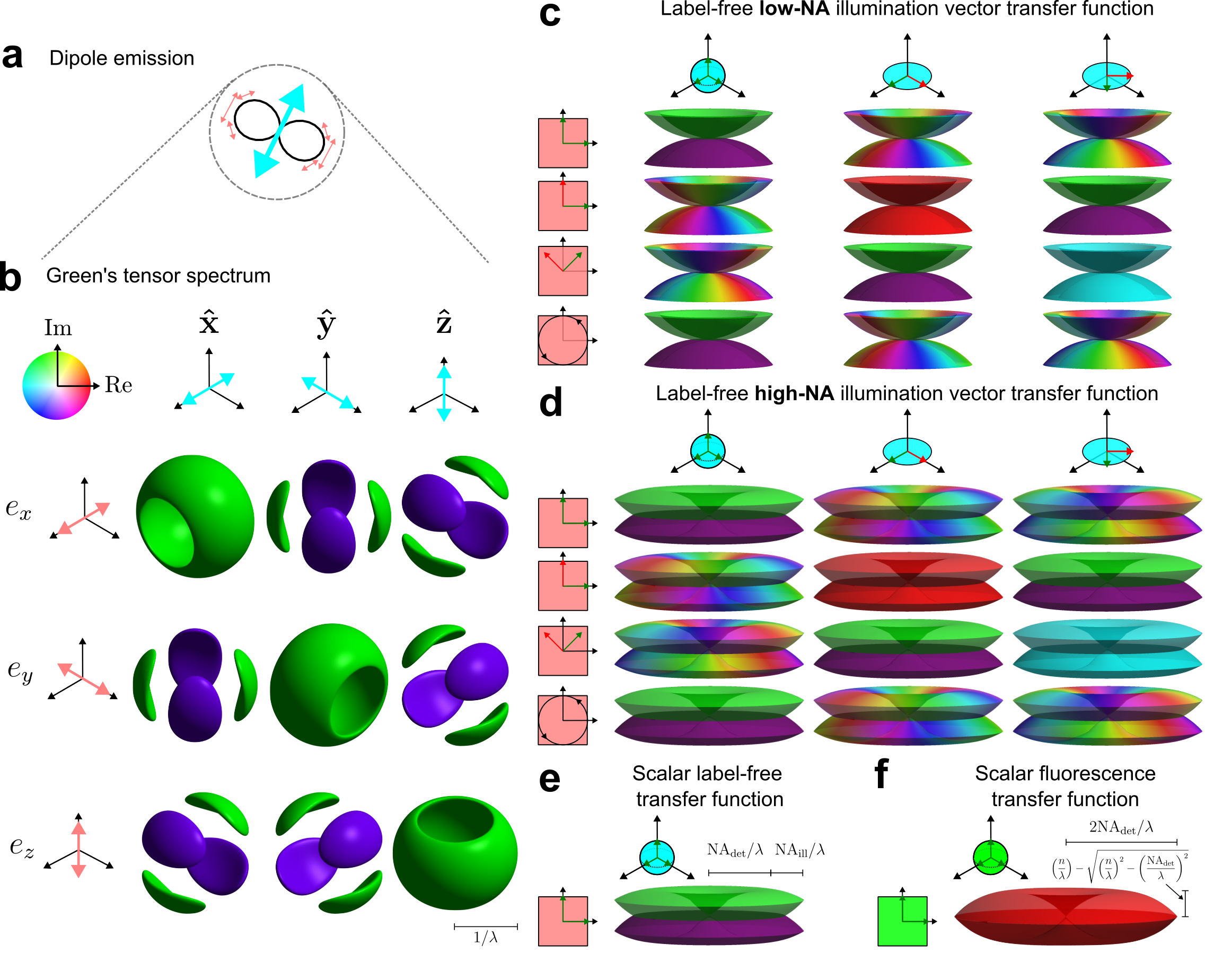
Figure 2: Key components of the forward model. (a) A dipole emitter (blue arrow) emits polarized fields (red arrows) in an anisotropic pattern (black line, radius proportional to power). (b) Arbitrary linear, circular, and elliptical dipole emissions can be modeled with the Green’s tensor spectrum $G_{ij}(\boldsymbol{\nu})$. Each surface shows the quarter-maximum intensity of on-shell spectral field components (rows) $e_{x}$, $e_{y}$, and $e_{z}$ emitted by dipoles oriented along (columns) $\hat{\textbf{x}}$, $\hat{\textbf{y}}$, and $\hat{\textbf{z}}$, with relative phase shown in color (see color rose). Orthogonal slices through the Green’s tensor spectrum and the Green’s tensor are shown in Figure S3. (c–f) 3D support of various transfer functions with phase encoded in color. (c-d) Real label-free vector transfer functions with $\text{NA}_{\text{det}}=0.75$ and circularly polarized illumination that expresses polarization-resolved data (rows) as outputs of filters that modulate material properties (columns) with (c) low-NA illumination $\text{NA}_{\text{ill}}=0.1$ and (d) high-NA illumination $\text{NA}_{\text{ill}}=0.5$. (e) Scalar label-free transfer function with $\text{NA}_{\text{ill}}=0.5$ and $\text{NA}_{\text{det}}=0.75$. (f) Scalar fluorescence transfer function with $\text{NA}_{\text{det}}=0.75$. See also Video 2.

All transfer functions can be expressed as products and autocorrelations of the illumination, scattering, and detection models, see Table 1 and Supplement 8. We refer to the complete transfer functions as vector models because they account for the complete vectorial nature of light and dipole scattering. We also include scalar models that ignore vector effects, which are reasonable approximations when unpolarized illumination and unpolarized detection are used on isotropic samples.

	vector	scalar
label-free	$\begin{bmatrix}H^{(\text{lf,re})}_{cp}(\boldsymbol{\nu})\\ H^{(\text{lf,im})}_{cp}(\boldsymbol{\nu})\end{bmatrix}=\sigma_{c}^{ii^{\prime}}\begin{bmatrix}1&1\\ \text{i}&-\text{i}\end{bmatrix}\begin{bmatrix}[P_{ij}G_{jn}\star P_{i^{\prime}k^{\prime}}S_{k^{\prime}}S^{*}_{k}](\boldsymbol{\nu})\\ [P_{ik^{\prime}}S_{k^{\prime}}S^{*}_{k}\star P_{i^{\prime}j}G_{jn}](\boldsymbol{\nu})\end{bmatrix}\mathcal{Y}_{p}^{nk}$	$\begin{bmatrix}H^{(\text{lf,re,s})}(\boldsymbol{\nu})\\ H^{(\text{lf,im,s})}(\boldsymbol{\nu})\end{bmatrix}=\begin{bmatrix}1&1\\ \text{i}&-\text{i}\end{bmatrix}\begin{bmatrix}[P\star PS](\boldsymbol{\nu})\\ [PS\star P](\boldsymbol{\nu})\end{bmatrix}$
fluorescence	$H^{(\text{fl})}_{cp}(\boldsymbol{\nu})=\sigma_{c}^{ii^{\prime}}[P_{ij}G_{jk}\star P_{i^{\prime}j^{\prime}}G_{j^{\prime}k^{\prime}}](\boldsymbol{\nu})\mathcal{Y}_{p}^{kk^{\prime}}$	$H^{(\text{fl,s})}(\boldsymbol{\nu})=[P\star P](\boldsymbol{\nu})$

Table 1: Transfer functions for different contrast modes (rows) and optical models (columns) expressed in terms of the illumination model $S$, the scattering model $G$, the detection model $P$, the object-space basis $\mathcal{Y}$, and the data-space basis $\sigma$. Sums over $i,i^{\prime},j,j^{\prime},k$ and $k^{\prime}$ are implied.

Figures 2c–f show the support and phase of several examples of waveOrder’s transfer functions. We briefly highlight several key features

• vector models consist of a grid of transfer functions, one for each data channel and material property,

• scalar models consist of a single transfer function, and

• we model real-valued data, so our transfer functions are Hermitian, that is $H_{cp}^{(m)}(\boldsymbol{\nu})=H_{cp}^{*(m)}(-\boldsymbol{\nu})$.

4 Multi-contrast multi-channel reconstructions across length scales

4.1 Label-free simulated and real test specimen

We tested our newly developed anisotropic label-free model on polarization-diverse data acquired from a laser-etched anisotropy phantom with transverse radially anisotropic bubbles arranged in a spoke pattern (Figure 3a,i). We measured four volumetric Stokes datasets (Figure 3a,ii) and applied waveOrder’s reconstruction algorithm to estimate three label-free material properties that correspond to phase and transverse birefringence (Figure 3a,iii).

In parallel, we simulated the anisotropic phantom (Figure 3b,i) and the image formation process (Figure 3b,ii), then we applied an identical reconstruction algorithm to estimate material properties (Figure 3b,iii). Figures 3a, ii-ii and b,ii–iii can be directly compared to indicate the quality of our models, where differences can arise from imperfect modeling of both the object and the image formation process. While our simulations recreate the most important contrast features, the real measurements have contrast with a broader axial extent and poorer transverse spatial resolution than our simulations—likely due to imperfections in our phantom and slightly aberrated imaging.

We compared an earlier ray-optics based voxel-by-voxel reconstruction algorithm [3] with waveOrder’s new wave optical reconstruction algorithm Figure 3c. We find that wave-optical reconstructions yield marginally improved transverse resolution Figure 3d measured via transverse modulation transfer functions from azimuthal profiles, and denoised and defocus-symmetric axial profiles Figure 3e. We also observe orientation reversals between spokes, reconstruction artifacts that are analogous to well-known negative ringing artifacts in fluorescence deconvolution.

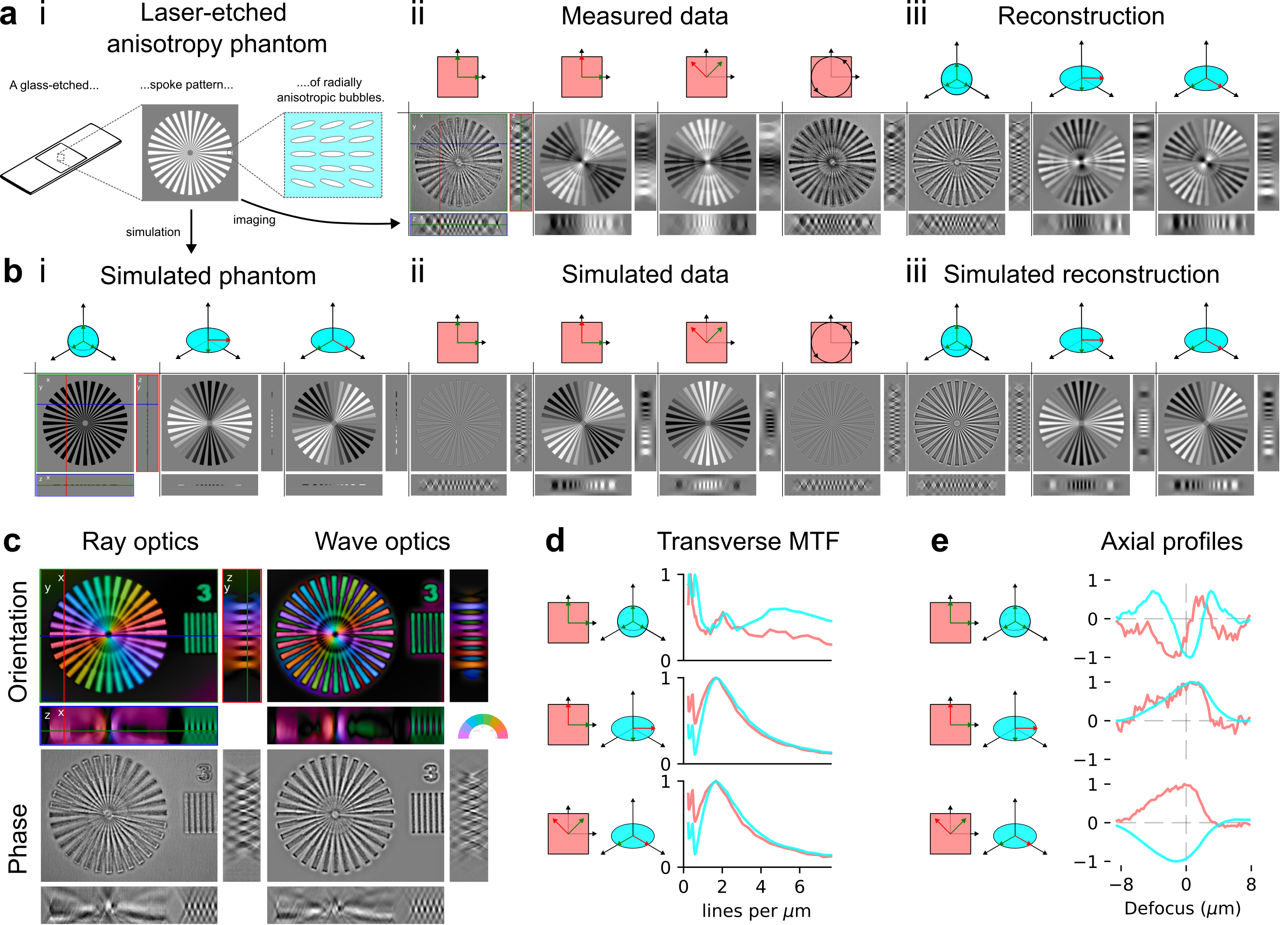
Figure 3: Demonstration of vectorial multi-channel reconstruction with experiment and simulation. We imaged (a) (i) a laser-etched spoke pattern of transverse radially anisotropic bubbles. (ii) We made volumetric measurements of the Stokes parameters (columns), and applied a multi-channel label-free reconstruction to (iii) recover material properties. (b) We (i) simulated the phantom’s material properties, (ii) simulated the imaging process, then (iii) simulated the reconstruction. (c) We encoded transverse birefringence properties into color, where brightness indicates the strength of the anisotropy and hue indicate the slow-axis orientation. We compared the orientation and phase reconstructions (rows) in ray- and wave-optics reconstructions (columns). (d) For each data and material property, we measured a series of azimuthal profiles at different radii on the spoke pattern and used the 10th–90th percentile modulation as an empirical estimate of the transverse modulation transfer function (MTF). (e) Similarly, we measured axial profiles through each data and material property. See also Video 3.

4.2 Cells and tissues

We applied waveOrder reconstructions to multi-channel data acquired from samples across length scales. Figure 4 shows alternating columns of data and reconstructions for transverse birefringence, phase, and fluorescence density. In data acquired from A549 cells (Figure 4a) we observe improved sectioning, denoising, and contrast in phase and reconstructed fluorescence properties compared to their raw-data counterparts (Figure 4a, ii–iii). In the orientation channel (Figure 4a, i) we observe marginal improvements in contrast, but generally poor performance with reduced SNR and suppression of features that are apparent in the raw data. We attribute some of the performance drop to our imperfect noise model—we reconstruct from non-Gaussian Stokes parameters which is at odds with our Tikhonov least-squares reconstruction algorithm. Additionally, we have not explored the interaction between our Stokes-based background correction and our wave-optical reconstructions, another likely area for improvement.

We acquired multi-contrast data from an entire living zebrafish (Figure 4b), then reconstructed fluorescence density, phase, and birefringence from specific regions of interest (Figure 4c–e). We observe improved sectioning, denoising, and contrast in all three reconstructions. For example, in the label-free Figure 4i, c–e we see improved contrast between the gut and muscles, and in the fluorescence channels Figure 4iii, c–e we see improved contrast and resolution of immune cells. Improved contrast in the zebrafish gut (bottom of Figure 4c) is particularly valuable for tracking immune-cell dynamics encoded in the fluorescence reconstructions.

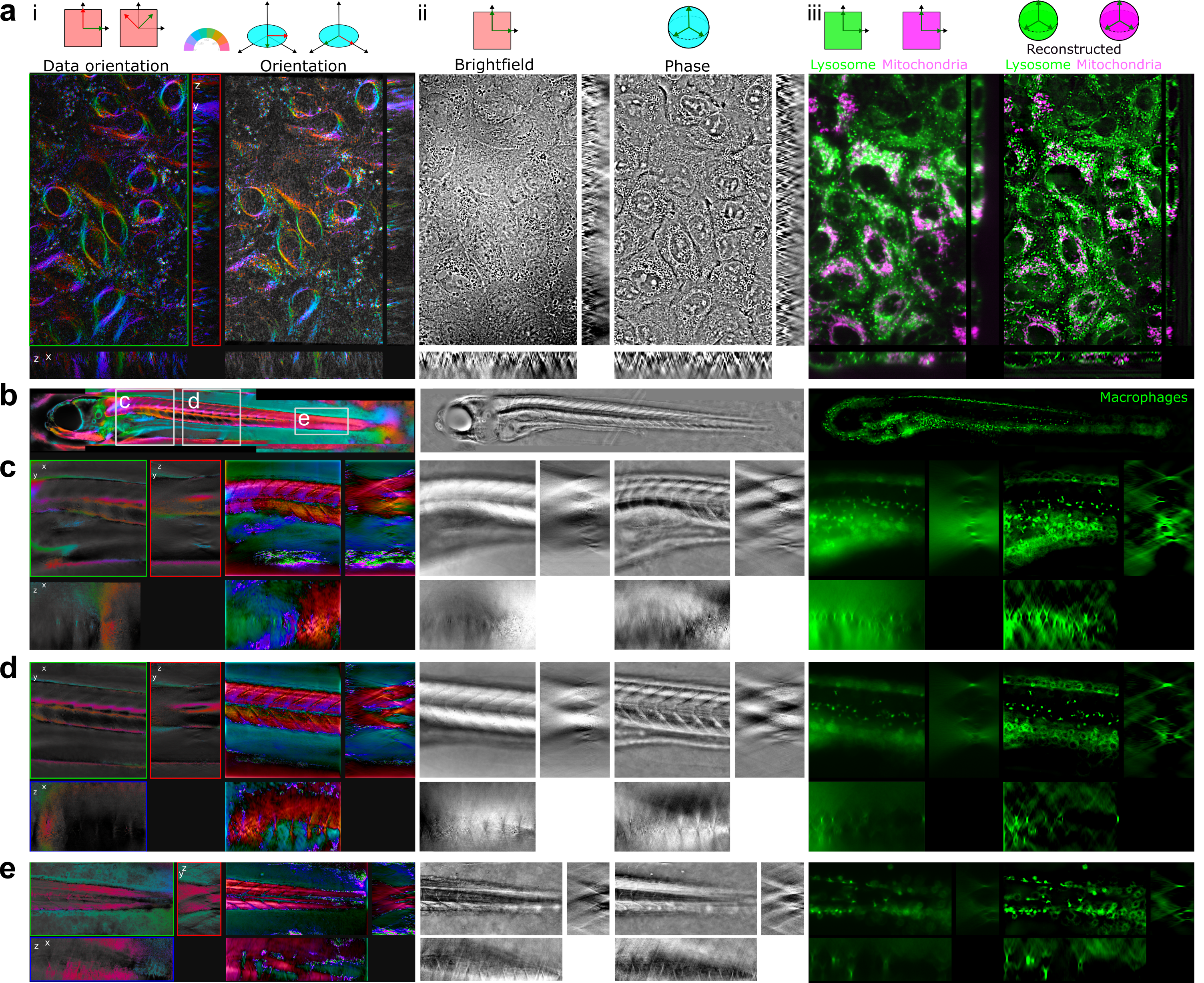
Figure 4: Reconstructions improve visualization and interpretation across length scales in (a) A549 cells, (b) zebrafish, and (c–e) zebrafish regions of interest. (i) Orientation data (left) and reconstructions (right). (ii) Brightfield data (left) and phase reconstructions (right). (iii) Fluorescence data (left) and reconstructions (right). See also Videos 4 and 5.

4.3 Choice of regularization parameter

waveOrder’s physics-informed reconstructions rely on a list of fixed parameters that specify imaging conditions (e.g., numerical apertures, wavelength, voxel sizes) and a single regularization parameter $\eta$, which penalizes large solutions and suppresses noise. Though [35, 36], in practice, it is common to inspect a regularization sweep and choose an empirical solution (for example, Figure 5 and Figure S1). Regularization parameters that are too small result in noisy reconstructions, while regularization parameters that are too large result in blurry reconstructions. Additionally, we find that the transverse mid-band power, the power in transverse spatial frequencies between one-eighth and one-quarter of the cutoff, is a useful scalar metric that can indicate high-quality reconstructions—see the plateau in Figure 5(d).

waveOrder’s current design uses a single regularization parameter per contrast mode. For example, we use one regularization parameter for each fluorescence deconvolution, one for each phase-from-brightfield reconstruction, and one for each joint reconstruction of phase and orientation. These single-parameter Tikhonov-regularized least squares reconstructions assume that all measured channels have an SNR proportional to their intensity and that the physical model accurately describes the differences in intensity between channels. This requirement becomes challenging when reconstructing directly from Stokes parameters, typically estimated with varying SNR. For example, the Stokes parameters that preceded the reconstruction in Figure 5 include a very noisy $S_{3}$. Here, we dropped $S_{3}$ from our dataset, ignoring its small contribution, but improved reconstructions with channel-specific regularization parameters may allow us to use this channel more effectively.

In future work, we are excited to pursue data-adaptive and channel-adaptive regularization in a data- and task-dependent manner. We are especially excited by methods that can address model mismatch, which often limits the quality of our reconstructions. For example, while Figure 5(iii,b–e) shows improved contrast and sectioning, model mismatch limits the quality of our reconstructions by leaving artifactual double cones throughout the reconstruction, particularly visible as transverse rings from bright out-of-focus cells.

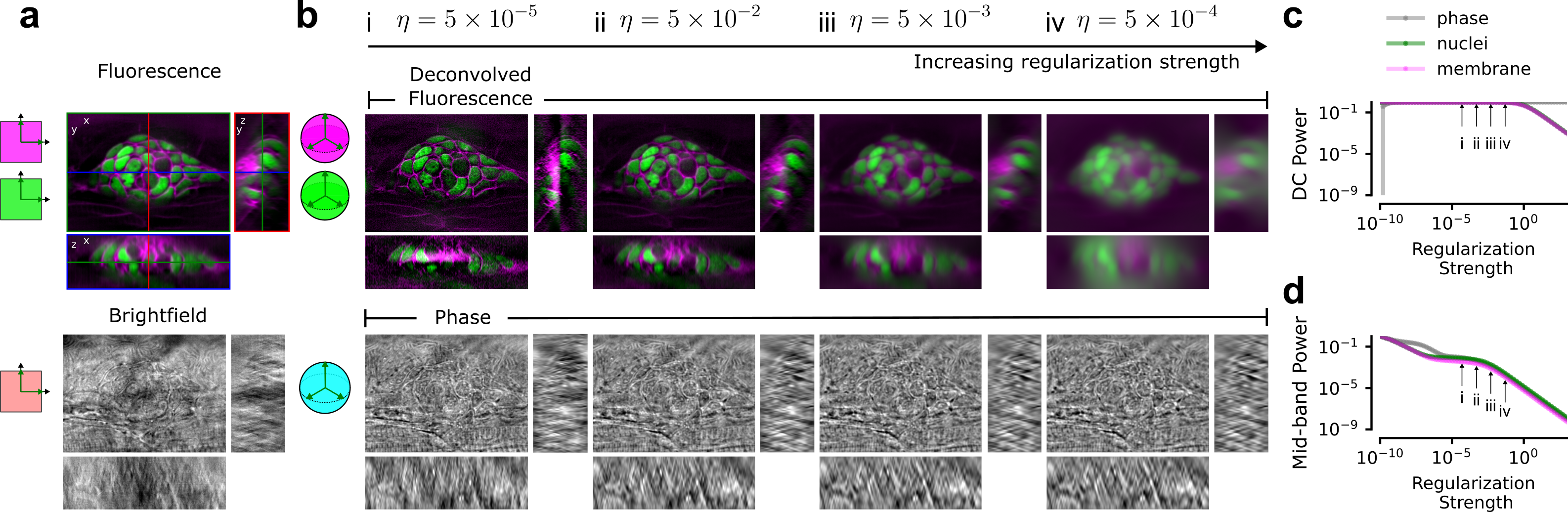
Figure 5: Effect of regularization parameter on reconstructions. (a) Zebrafish neuromasts imaged in fluorescence and brightfield channels are (b) reconstructed over a range of regularization parameters, with small parameters generating noisy results and large parameters generating blurred results. Near the empirically selected optimal reconstruction (b, ii), the DC power (c) is nearly constant. In contrast, the mid-band power (d), the power for transverse spatial frequencies between one-eighth and one-quarter of the cutoff, changes when the regularization parameter is too high or too low and plateaus when the regularization parameter is in the correct range.

5 Limitations

While waveOrder enables the development of image formation models and reconstruction algorithms for a wide variety of computational microscopy techniques, its current design makes the following assumptions that are not valid in certain applications:

• consistent SNR in all channels, which assumes that all data channels that encode a given contrast have a similar signal-to-noise ratio.

• channel linearity, which excludes non-linear crosstalk between channels e.g. FRET, strongly scattering samples,

• spatial linearity, which excludes saturation of fluorescent samples or the camera,

• shift invariance, which excludes shift-variant point spread functions [37],

• weak, single scattering, which excludes thick multiply scattering samples [38], e.g. older zebrafish and thick tissue slices,

• aberration-free imaging, which excludes applications in the presence of sample-induced aberrations.

• contrast-separable imaging, which excludes crosstalk between label-free and fluorescence contrast modes [39].

6 Discussion and conclusion

waveOrder improves on earlier multi-channel correlative imaging methods in several ways. Compared to LC-PolScope reconstruction methods [40], waveOrder uses a wave-optical approach that reconstructs from diffraction-limited groups of voxels instead of reconstructing voxel by voxel. waveOrder also extends quantitative label-free imaging with phase and polarization (QLIPP) [3], by using a vectorial wave-optics model of multiple specimen properties, not just phase. waveOrder also extends permittivity tensor imaging (PTI) [21], which reconstructs only uniaxial permittivity tensors while waveOrder is compatible with arbitrary biaxial materials. The waveOrder framework also generalizes previous work on imaging polarized fluorescence ensembles [14, 24], where diffraction-limited ensembles of fluorescent dipoles reduce to orientation distribution functions. As discussed earlier, we view careful noise handling and more robust background correction as areas for future work.

To conclude, we find that linear models provide a strong framework for widely applicable computational microscopy techniques, including phase, absoprtion, birefringence, diattenuation, and anistropic fluorescence imaging. We find the waveOrder framework useful for understanding, simulating, and reconstructing data acquired with this class of techniques, and we demonstrate its ability to improve multi-contrast multi-channel data across length scales.

7 Data and code availability

Demos, data and code can be found in the recOrder and
waveOrder repositories.

8 Acknowledgements

We thank Shashvat Mehta for developing the animation shown in Video 1. We thank the Scientific Computing Platform at CZ Biohub for enabling high-performance reconstructions.

9 Funding

All authors are supported by intramural funding from Chan Zuckerberg Biohub, San Francisco, an institute funded by the Chan Zuckerberg Initiative. We thank Priscilla Chan and Mark Zuckerberg for supporting the CZ Biohub Network.

10 Disclosures

The authors declare no conflicts of interest.

References

- [1] R. Schlüßler, K. Kim, M. Nötzel, et al., “Correlative all-optical quantification of mass density and mechanics of subcellular compartments with fluorescence specificity,” \JournalTitleeLife 11, e68490 (2022). Publisher: eLife Sciences Publications, Ltd.
- [2] I. E. Ivanov, E. Hirata-Miyasaki, T. Chandler, et al., “Mantis: High-throughput 4D imaging and analysis of the molecular and physical architecture of cells,” \JournalTitlePNAS Nexus 3, 323 (2024).
- [3] S.-M. Guo, L.-H. Yeh, J. Folkesson, et al., “Revealing architectural order with quantitative label-free imaging and deep learning,” \JournalTitleeLife 9, e55502 (2020).
- [4] E. Gómez-de Mariscal, M. Del Rosario, J. W. Pylvänäinen, et al., “Harnessing artificial intelligence to reduce phototoxicity in live imaging,” \JournalTitleJournal of Cell Science 137, jcs261545 (2024).
- [5] Z. Liu, E. Hirata-Miyasaki, S. Pradeep, et al., “Robust virtual staining of landmark organelles,” (2024).
- [6] B. Yang, M. Lange, A. Millett-Sikking, et al., “DaXi—high-resolution, large imaging volume and multi-view single-objective light-sheet microscopy,” \JournalTitleNature Methods 19, 461–469 (2022). Publisher: Nature Publishing Group.
- [7] E. Sapoznik, B.-J. Chang, J. Huh, et al., “A versatile oblique plane microscope for large-scale and high-resolution imaging of subcellular dynamics,” \JournalTitleeLife 9, e57681 (2020). Publisher: eLife Sciences Publications, Ltd.
- [8] K. H. Chen, A. N. Boettiger, J. R. Moffitt, et al., “Spatially resolved, highly multiplexed RNA profiling in single cells,” \JournalTitleScience 348, aaa6090 (2015). Publisher: American Association for the Advancement of Science.
- [9] S. Black, D. Phillips, J. W. Hickey, et al., “CODEX multiplexed tissue imaging with DNA-conjugated antibodies,” \JournalTitleNature Protocols 16, 3802–3835 (2021). Publisher: Nature Publishing Group.
- [10] T. Kudo, A. M. Meireles, R. Moncada, et al., “Multiplexed, image-based pooled screens in primary cells and tissues with PerturbView,” \JournalTitleNature Biotechnology pp. 1–10 (2024). Publisher: Nature Publishing Group.
- [11] D. Serwas and K. M. Davies, “Getting Started with In Situ Cryo-Electron TomographyCryo-electron tomography (Cryo-ET),” in cryoEM: Methods and Protocols, T. Gonen and B. L. Nannenga, eds. (Springer US, New York, NY, 2021), pp. 3–23.
- [12] J. A. Pierson, J. E. Yang, and E. R. Wright, “Recent advances in correlative cryo-light and electron microscopy,” \JournalTitleCurrent Opinion in Structural Biology 89, 102934 (2024).
- [13] A. S. Backer and W. E. Moerner, “Extending Single-Molecule Microscopy Using Optical Fourier Processing,” \JournalTitleThe Journal of Physical Chemistry B 118, 8313–8329 (2014).
- [14] T. Chandler, H. Shroff, R. Oldenbourg, and P. La Rivière, “Spatio-angular fluorescence microscopy I Basic theory,” \JournalTitleJournal of the Optical Society of America A 36, 1334 (2019).
- [15] N. Streibl, “Three-dimensional imaging by a microscope,” \JournalTitleJournal of the Optical Society of America A 2, 121 (1985).
- [16] Y. Bao and T. K. Gaylord, “Quantitative phase imaging method based on an analytical nonparaxial partially coherent phase optical transfer function,” \JournalTitleJournal of the Optical Society of America A 33, 2125 (2016).
- [17] P. Török, “Imaging of small birefringent objects by polarised light conventional and confocal microscopes,” \JournalTitleOptics Communications 181, 7–18 (2000).
- [18] R. Oldenbourg and P. Török, “Point-spread functions of a polarizing microscope equipped with high-numerical-aperture lenses,” \JournalTitleApplied Optics 39, 6325 (2000).
- [19] A. Saba, J. Lim, A. B. Ayoub, et al., “Polarization-sensitive optical diffraction tomography,” \JournalTitleOptica 8, 402–408 (2021). Publisher: Optical Society of America.
- [20] S. Shin, J. Eun, S. S. Lee, et al., “Tomographic measurement of dielectric tensors at optical frequency,” \JournalTitleNature Materials 21, 317–324 (2022). Number: 3 Publisher: Nature Publishing Group.
- [21] L.-H. Yeh, I. E. Ivanov, T. Chandler, et al., “Permittivity tensor imaging: modular label-free imaging of 3D dry mass and 3D orientation at high resolution,” \JournalTitleNature Methods pp. 1–18 (2024). Publisher: Nature Publishing Group.
- [22] H. Jang, Y. Li, A. A. Fung, et al., “Super-resolution SRS microscopy with A-PoD,” \JournalTitleNature Methods 20, 448–458 (2023).
- [23] O. Zhang, Z. Guo, Y. He, et al., “Six-dimensional single-molecule imaging with isotropic resolution using a multi-view reflector microscope,” \JournalTitleNature Photonics 17, 179–186 (2023).
- [24] T. Chandler, M. Guo, Y. Su, et al., “Three-dimensional spatio-angular fluorescence microscopy with a polarized dual-view inverted selective-plane illumination microscope (pol-diSPIM),” (2024).
- [25] H. H. Hopkins, “The concept of partial coherence in optics,” \JournalTitleProceedings of the Royal Society of London. Series A. Mathematical and Physical Sciences 208, 263–277 (1951).
- [26] H. H. Barrett and K. J. Myers, Foundations of image science, Wiley series in pure and applied optics (Wiley-Interscience, Hoboken, NJ, 2004).
- [27] S. B. Mehta and C. J. R. Sheppard, “Partially coherent microscope in phase space,” \JournalTitleJournal of the Optical Society of America A 35, 1272 (2018).
- [28] C. J. R. Sheppard, “Partially coherent microscope imaging system in phase space: effect of defocus and phase reconstruction,” \JournalTitleJournal of the Optical Society of America A 35, 1846 (2018).
- [29] E. Wolf, Introduction to the theory of coherence and polarization of light (Cambridge Univ. Press, Cambridge, 2007), 1st ed.
- [30] M. A. Bruce and M. J. Butte, “Real-time GPU-based 3D Deconvolution,” \JournalTitleOptics Express 21, 4766 (2013).
- [31] E. Wernersson, E. Gelali, G. Girelli, et al., “Deconwolf enables high-performance deconvolution of widefield fluorescence microscopy images,” \JournalTitleNature Methods 21, 1245–1256 (2024).
- [32] K. Herath, U. Haputhanthri, R. Hettiarachchi, et al., “Differentiable Microscopy Designs an All Optical Phase Retrieval Microscope,” (2022).
- [33] D. Deb, G.-J. Both, A. Chaware, et al., “Chromatix: a high-performance differentiable wave optics simulation library,” in Computational Optics 2024, D. G. Smith and A. Erdmann, eds. (SPIE, Strasbourg, France, 2024), p. 45.
- [34] O. Zhang and M. D. Lew, “Single-molecule orientation localization microscopy I: fundamental limits,” \JournalTitleJournal of the Optical Society of America A 38, 277 (2021).
- [35] P. C. Hansen, “The L-curve and its use in the numerical treatment of inverse problems,” (2005).
- [36] T. H. Edwards and S. Stoll, “Optimal Tikhonov regularization for DEER spectroscopy,” \JournalTitleJournal of Magnetic Resonance 288, 58–68 (2018).
- [37] K. Yanny, K. Monakhova, R. W. Shuai, and L. Waller, “Deep learning for fast spatially varying deconvolution,” \JournalTitleOptica 9, 96 (2022).
- [38] R. Bartels and O. Pinaud, “Analysis and extensions of the Multi-Layer Born method,” (2024). ArXiv:2412.07983 [physics].
- [39] Y. Xue, D. Ren, and L. Waller, “Three-dimensional bi-functional refractive index and fluorescence microscopy (BRIEF),” \JournalTitleBiomedical Optics Express 13, 5900 (2022).
- [40] S. B. Mehta, M. Shribak, and R. Oldenbourg, “Polarized light imaging of birefringence and diattenuation at high resolution and high sensitivity,” \JournalTitleJournal of Optics 15, 094007 (2013).