A Differentiable Wave Optics Model for End-to-End Computational Imaging System Optimization

Abstract

End-to-end optimization, which simultaneously optimizes optics and algorithms, has emerged as a powerful data-driven method for computational imaging system design. This method achieves joint optimization through backpropagation by incorporating differentiable optics simulators to generate measurements and algorithms to extract information from measurements. However, due to high computational costs, it is challenging to model both aberration and diffraction in light transport for end-to-end optimization of compound optics. Therefore, most existing methods compromise physical accuracy by neglecting wave optics effects or off-axis aberrations, which raises concerns about the robustness of the resulting designs. In this paper, we propose a differentiable optics simulator that efficiently models both aberration and diffraction for compound optics. Using the simulator, we conduct end-to-end optimization on scene reconstruction and classification. Experimental results demonstrate that both lenses and algorithms adopt different configurations depending on whether wave optics is modeled. We also show that systems optimized without wave optics suffer from performance degradation when wave optics effects are introduced during testing. These findings underscore the importance of accurate wave optics modeling in optimizing imaging systems for robust, high-performance applications.

1 Introduction

The interdependence between optics and downstream algorithms is pivotal in imaging system design. To leverage this interdependence and achieve joint designs, end-to-end differentiable models, which incorporate a differentiable optics simulator and a computer vision algorithm, have been applied to simultaneously optimize hardware and software across a range of vision tasks [7, 33, 28, 32, 26, 21, 27, 25]. Given a dataset of training images, the differentiable optics simulator models corresponding measurements taken by the optics system, and the computer vision algorithm extracts information from simulated measurements. Because both the simulator and algorithm are differentiable, a loss function scores task performance and drives the optimization of the optics and algorithm parameters via backpropagation.

A notable challenge in end-to-end optimization is incorporating wave optics effects in large field-of-view (FoV) and analyzing how the fidelity of optics simulation impacts overall system optimization. Computational expense imposes a limitation on exploring the effects of realistic optical modeling, particularly when integrating wave optics. To accurately capture wave optics effects, simulations must model the contribution of each ray across the entire sensor rather than simply tracing its path. This complexity intensifies as the number of rays and sensor pixels increases. Therefore, many end-to-end designs simplify the physics models and use ray optics, which neglects diffraction, to simulate light transport [7, 27, 33]. Even though some simulators do take diffraction into account, they still make assumptions of thin-phase surfaces [25, 31] or shift-invariance [26, 3, 13]. These approaches fail to model realistic multi-element and compound optics designs, limiting the space of possible lens designs. Although recent frameworks model wave optics [6, 34], the efficiency of differentiable engines and the significance of wave optics effects on system optimization still remain open problems.

In this paper, we propose a differentiable optics simulator, which forgoes thin-phase approximations and modeling off-axis aberrations and wave optical effects in compound optical systems. To address the computation costs of simulating diffraction and aberrations over the entire FoV, we use an interpolation method to approximate the measurements with a subset of point spread functions (PSFs). By providing accurate and efficient wave optics rendering, the proposed simulator enables us to incorporate wave optics effects into end-to-end optimization, assess their impact on system design, and identify scenarios where wave optics play a critical role in optimizing imaging performance.

Unlike systems optimized solely under ray optics assumptions, our diffraction-aware simulator guides lens systems toward configurations with lower F-numbers, effectively balancing diffraction blur and controllable aberrations during end-to-end optimization. By accurately accounting for wave optics effects, this approach achieves up to 16% lower reconstruction error and 23% higher classification accuracy compared to systems optimized without considering diffraction, resulting in significantly improved image quality.

Our contributions are

• We propose a differentiable simulator that models aberration and diffraction in compound optical systems with state-of-the-art accuracy, efficiently rendering measurements by leveraging isoplanatic properties among PSFs.

• We demonstrate that neglecting diffraction in end-to-end optimization leads to suboptimal lens and algorithm configurations. Conversely, by accurately capturing diffraction effects, our model attains superior solutions to image reconstruction and classification.

• We show that wave optics modeling is especially impactful in end-to-end design for systems with small pixel sizes and weakly aberrated optics.

2 Related Work

2.1 End-to-End Optimization.

Conventional lens designs construct a merit function, which combines lens properties and transfer function quality, to optimize optics systems [19]. Nonetheless, the merit functions are not guaranteed to reflect computer vision task performance [9, 33]. Therefore, end-to-end optimizations use task performance to optimize hardware and software concurrently. Through the cooperation between differentiable optics simulators and inference algorithms on a large dataset [27, 7, 33, 13], end-to-end optimization provides a data-driven design that addresses the interdependence among optics, algorithms, and tasks[9].

End-to-end optimization has been widely applied to image reconstruction [26, 21, 25, 9, 18, 17] and restoration [11, 36]. Sitzmann et al. extend the depth of field on computational cameras [26]. Peng et al. achieve high FOV image reconstruction [21]. Shi et al. recover unobstructed scenes by a diffractive optical element and point-PSF-aware neural network [25]. The strategy has also been applied to semantic information extraction. Baek et al. acquire depth information from hyperspectral imaging by jointly optimizing diffractive optical elements and a deep network [3]. Kellman et al. recover phase information by jointly optimizing coded-illumination patterns for an LED array and an unrolled physics-based network [15]. Pidhorskyi et al. develop a differentiable ray tracer for depth-of-field aware scene intensity recovery [22]. Yang et al. optimize off-axis aberration performance for image classification [33]. Cote et al. optimize lens materials and structures for object detection [7]. In all of these frameworks, end-to-end optimization enables the system to specialize in a particular vision application.

2.2 Physics Models in Optics Simulation

A notable concern in end-to-end optimization is the computational cost of optics simulation [34, 30]. Because end-to-end design usually requires complex physics simulation to generate measurements from a large imaging dataset, complicated gradient propagations are needed to model the relation among optics parameters, measurements, and semantic information [30]. To address the cost in large FOV differentiable rendering, simplified physics models are usually adopted. Peng et al. adopt the thin phase assumption to optimize thin-plate lens in large FOV imaging reconstruction [21]. Sun et al. use ray optics to model differentiable ray tracing in complex lens model [27]. Cote et al. use ray optics with ray aiming to improve the accuracy of simulating lenses with strong pupil aberrations [7]. Although these methods manage to reduce the computation costs, their approaches cannot model wave optical effects.

It is also common to model wave optical effects under strong assumptions. Sitzmann et al. use Fresnel propagation to model wave optics in diffractive optics but assume the system is shift-invariant [26]. Shi et al. incorporates diffractive optics and a lens using the thin phase assumption [25]. He et al. compute PSFs with diffraction theory in shift-variant systems [13]. Tseng et al. replace the entire physics simulator and imaging pipeline with a neural network to render PSFs [29]. Wei et al. model off-axis diffraction using the angular spectrum method [31], but assume the system is a thin-phase single lens. All these assumptions limit their applicability to compound optical systems.

Chen et al. [6] developed a ray-wave optics simulator that evolves from Zemax PSF simulation [19] and calculates the diffraction at the exit pupil, but the framework is not differentiable or applicable to end-to-end optimization. A concurrent pre-print work by Yang et al. optimizes a hybrid lens-diffractive optic system [34] with a well-known approach implemented in many commercial packages, such as Code V and Zemax OpticStudio, but does not explore the difference between ray and wave models during lens and network training. In our work, we adopt a differentiable rendering method that models diffraction from rays and uses it to explore the impacts of the improved accuracy of a wave model in end-to-end design. We show that a full FoV wave optics rendering model can lead to meaningfully different designs compared with a ray-only model.

3 Differentiable Optics Model

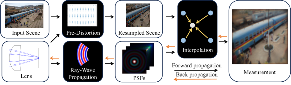
Figure 1: The block diagram of the proposed differentiable wave optics simulation. Black blocks indicate operations, while white blocks indicate inputs, outputs, or intermediate products.

Our differentiable simulator is designed to accurately capture both aberration and diffraction in compound optics systems, making it a robust model for data-driven computational imaging system design. Its efficiency in forward and backward propagation across multiple scene batches enables scalable end-to-end optimization, thus enhancing overall imaging performance.

To achieve high fidelity in physical modeling, we utilize a hybrid ray-wave model described in Sec. 3.1. This model takes a differentiable ray tracer as the backbone [30] while accurately accounting for wave optics effects through optical path length calculations. Specifically, for a point light source at $\mathbf{x}=(x,y,z)$ with intensity $b(\mathbf{x})$, and an optical system with sequential refractive surfaces, the ray-wave model computes the PSF $h(\mathbf{u}|\mathbf{x})$, where $\mathbf{u}$ denotes sensor pixel position. The resulting measurement $I(\mathbf{u})$ is derived from the superposition integral [6]:

$$I(\mathbf{u})=\int b(\mathbf{x})h(\mathbf{u}|\mathbf{x})d\mathbf{x}.$$ (1)

However, directly computing Eq. 1 across the entire FoV is computationally intensive, requiring full-resolution PSF rendering for every point source. To address this challenge, we develop an efficient interpolation method that balances accuracy and computational cost. The approach involves sampling a subset of PSFs and using interpolation to approximate the full measurement with a manageable number of convolutions [4], effectively capturing diffraction, off-axis aberrations, and geometric distortions. By achieving state-of-the-art accuracy in optical modeling, the simulator improves the robustness of data-driven lens design and allows for a deeper exploration of wave optics effects in imaging applications. Details of this interpolation technique are provided in Sec. 3.2.

3.1 PSF Rendering

A conceptual flow of PSF rendering is illustrated in Fig. 2. To compute a PSF, we first use geometric ray tracing to sample the wavefront map in the exit pupil, and then propagate the complex field of the wavefront map to the sensor plane. In ray tracing, we use Newton’s Method [27, 30] to calculate the intersections between rays and surfaces and use Snell’s Law to model refractions. The wavefront map is then calculated in the reference sphere, whose center and radius are determined by the intersection between the chief ray and the sensor plane, and the distance between the exit pupil and the sensor, respectively.

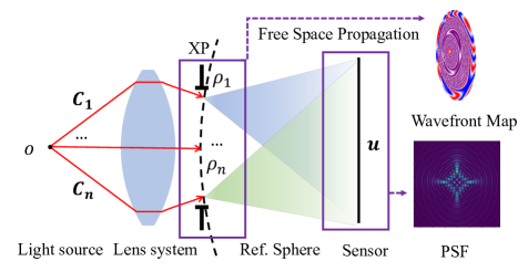
Figure 2: A conceptual flow of wave optics simulation. To model the wave optics propagation from point source $o$, we trace rays emitted from $o$ to the reference sphere in the system exit pupil, compute intersections $\{\bm{\rho}_{i}\}$ and associated phase to build a wavefront map. We then perform free-space propagation toward the sensor to generate a PSF. XP: Exit Pupil. Ref: Reference.

Therefore, the problem amounts to calculating the amplitude and phase of the complex field at the reference sphere. By noting that the exit pupil is an image of the aperture stop, we model the amplitude by the square root of the aperture stop transmittance. On the other hand, the phase at the reference sphere is determined by the optical path length (OPL) $\delta$ calculated by

$$\delta=\int_{C}n(s)ds{,}$$ (2)

where $n(s)$ is the 3D refractive index of the system and $C$ is the path that a given ray takes from the light source to the reference sphere [14].

It is notable that the phase across the reference sphere, called the wavefront error map, reflects the degree of focusing [24]. When the system is in-focus, the reference sphere exactly matches the wavefront, and the phase is constant on the sphere. Otherwise, the mismatch between the actual wavefront and the reference sphere causes phase variations across the reference sphere. We choose to model the wavefront error map on the reference sphere because of its interpretability and compatibility with our propagation model, but the choice of the reference geometry is arbitrary and depends on the propagation model [24, 19].

Consequently, for a ray piercing the reference sphere at coordinate $\bm{\rho_{i}}=(\rho_{x_{i}},\rho_{y_{i}},\rho_{z_{i}})$, we model the complex field by

$$v(\bm{\rho}_{i})=a_{i}\exp{(jk\delta_{i})},$$ (3)

where $a_{i}$ is the amplitude, $k$ is the wave number, $j=\sqrt{-1}$, and $\delta_{i}$ is the optical path length.

As shown in Fig 2, the propagation from the reference sphere to the sensor is in free space. The total intensity, $h(\textbf{u})$, at sensor coordinate u is computed by the Rayleigh-Sommerfeld integral [10], which we Monte-Carlo evaluate with N rays by

$$h(\textbf{u})=\frac{1}{N\lambda^{2}}\Bigg{|}\sum_{i=1}^{N}v({\bm{\rho}_{i}})\frac{\exp{(jk|\vec{r}_{u,i}|)}}{|\vec{r}_{u,i}|}\cos(\theta_{u,i})\Bigg{|}^{2},$$ (4)

where $\vec{r}_{u,i}$ denotes the vector from $\bm{\rho}_{i}$ to sensor coordinate u, and $\theta_{u,i}$ is the angle between $\vec{r}_{u,i}$ and normal vector of the reference geometry at $\bm{\rho}_{i}$.

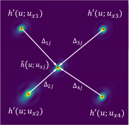
Figure 3: An illustration of how we exploit isoplanatic property among neighboring PSFs to approximate unsampled PSFs using Eq. 5. $h^{\prime}(u;u_{x1})$ to $h^{\prime}(u;u_{x4})$ denote sampled PSFs, and $\hat{h}(u;u_{xj})$ is an estimated PSF. All intensities are normalized.

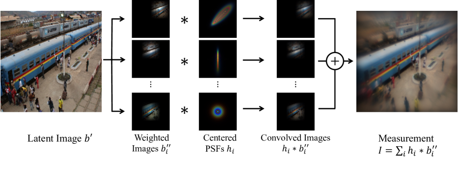
Figure 4: An illustration of interpolation in our system. We sample a subset of PSFs and convolve them with corresponding weighted scene intensities. The measurement is obtained by summing up all convolution results.

3.2 Approximating Superposition Integral

Although we can render PSFs with wave optics effects, the high computational costs make it challenging to exhaustively compute all PSFs. A common way to alleviate this cost is to assume the system is shift-invariant and approximate Eq. 1 with a single convolution between the on-axis PSF and scene intensities [10]. However, this assumption is overly restrictive as it does not model common off-axis aberrations such as coma, astigmatism, and field curvatures.

Therefore, we assume that PSFs are locally isoplanatic; the system is shift-invariant over a sufficiently small area. This allows us to sample a small subset of PSFs and approximate the superposition integral through a sequence of convolutions, thereby saving computational costs while maintaining the ability to model off-axis aberrations.

To facilitate the derivation, we parameterize scene intensities $b(\mathbf{x})$ and PSFs $h(\mathbf{u;x})$ in terms of sensor coordinates $\{\mathbf{u}\}$ as follows. For each world coordinate $\mathbf{x}$, we compute the intersection $\mathbf{u_{x}}$ between its non-paraxial chief ray and sensor plane, where the relation can be modeled by the lens distortion function $\mathbf{u_{x}}=d(\mathbf{x})$. Because the function is one-to-one, the scene intensities $b(\mathbf{x})$ and PSF $h(\mathbf{u;x})$ can be re-parameterized as $b^{\prime}(\mathbf{u_{x}})$ and $h^{\prime}(\mathbf{u;u_{x}})$, respectively. An example of distorted coordinates is visualized in Fig. 1. Because the distortion function $d(\mathbf{x})$ only determines the input scene content, we only consider it in the inference, but not in the back-propagation.

Fig. 3 shows an example of approximating a PSF originating from an unsampled world coordinate $\mathbf{x_{j}}$ according to PSFs $\{h(\mathbf{u};\mathbf{u_{xi}})\}$ originating from sampled world coordinates $\{\mathbf{x}_{i}\}$. For an unsampled PSF centered at $\mathbf{u_{xj}}$, we model it as the weighted sum of the known neighboring PSFs aligned at the same location:

$$\widehat{h}(\mathbf{u};\mathbf{u_{xj}})=\sum_{i}w_{i}(\mathbf{u_{xj}})h^{\prime}(\mathbf{u}-\Delta_{ij};\mathbf{u_{xi}}),$$ (5)

where $\Delta_{ij}=\mathbf{u_{xj}}-\mathbf{u_{xi}}$ is the center-to-center distance, in the sensor space, between the sampled PSF $i$ and unsampled PSF $j$. $w_{i}(\mathbf{u_{xj}})$ determines the weight of the sampled PSF $i$ when approximating the unsampled PSF centered at $\mathbf{u_{xj}}$.

We rewrite Eq. 1 by substituting the general form for the shift-varying PSFs found in Eq. 5:

$$I(\mathbf{u}) =\sum_{\mathbf{u_{x}}}b^{\prime}(\mathbf{u_{x}})\sum_{i}w_{i}(\mathbf{u_{x}})h^{\prime}(\mathbf{u}+\mathbf{u_{xi}}-\mathbf{u_{x}};\mathbf{u_{xi})}$$

$$=\sum_{i}\sum_{\mathbf{u_{x}}}b^{\prime\prime}_{i}(\mathbf{u_{x}})h^{\prime}(\mathbf{u}+\mathbf{u_{xi}}-\mathbf{u_{x}};\mathbf{u_{xi}}){,}$$ (6)

where $b^{\prime\prime}_{i}(\mathbf{u_{x}})=b^{\prime}(\mathbf{u_{x}})w_{i}(\mathbf{u_{x}})$ represents the weighted latent image, which are input scene intensities distorted by the lens distortion curve and weighted by $w_{i}(\cdot)$.

We observe that Eq. 6 is a sum of convolutions between the sampled PSFs, shifted to the origin, and the corresponding weighted latent image:

$$I(\mathbf{u}) =\sum_{i}\sum_{\mathbf{u_{x}}}b^{\prime\prime}_{i}(\mathbf{u_{x}})h_{i}(\mathbf{u}-\mathbf{u_{x}})$$

$$=\sum_{i}b^{\prime\prime}_{i}*h_{i}$$ (7)

where $h_{i}(\mathbf{u})=h^{\prime}(\mathbf{u+u_{i};u_{xi}})$. Fig. 4 illustrates an example of how we pair weighted images and PSFs, convolve them with each other, and sum up the convolved images to approximate the measurement.

Using the chain rule, gradients can be back-propagated from the measurements $I$ through the wave-optics PSFs $h(\textbf{u})$, the complex field $v(\bm{\rho}_{i})$ on the reference sphere, and ultimately to the lens parameters. This differentiability enables precise modeling and analysis of the interactions between lens configurations and wave-optics effects on the measurements. In the subsequent section, we incorporate this differentiable wave-optics simulator into computer vision algorithms, allowing analysis of the impact of wave-optics effects on optical systems tailored for vision tasks.

4 Experiments

With the simulator, we conduct joint optimization of optics systems and algorithms for scene reconstruction and image classification and analyze the importance of modeling diffraction in end-to-end optimization. To the best of our knowledge, this is an unexplored experimental flow that analyzes the requirements of physics accuracy in end-to-end optimization.

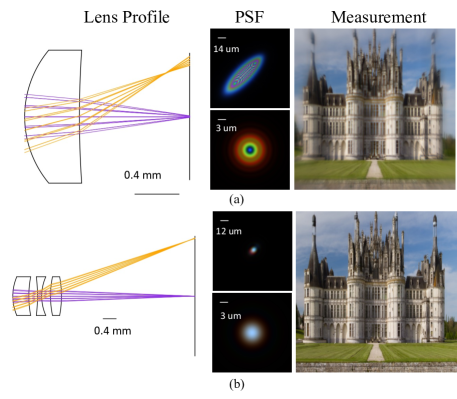
Figure 5: The PSFs and measurement generated by our simulator from (a) singlet lens (b) Cooke triplet lenses.

4.1 Wave Optics Rendering

We simulate PSFs and measurements obtained from singlet and Cooke triplet lenses in Fig. 5. The singlet lens demonstrates prominent effects from both diffraction and off-axis aberrations. The on-axis PSF shows clear diffraction fringes, while the off-axis shows a combination of coma and astigmatism with clear diffraction effects. The Cooke triplet lens, by nature of its optimized design, drastically reduces aberrations. The result is a PSF that is nearly diffraction-limited over the FoV. These results demonstrate how our model faithfully renders images for both aberration-limited and diffraction-limited systems, enabling end-to-end optimization of lenses across both regimes.

4.2 System Optimization Setup

We conduct end-to-end optimization experiments to co-design Cooke triplet lenses and imaging algorithms for two different tasks: scene reconstruction with Bayer filter array, and image classification. The Cooke triplet configuration consists of three lens elements (materials N-LAF2, N-SF10, and N-LAF2). For optimization, we employ the Adam optimizer [16] to drive the refinement of network parameters and curvatures of all lens surfaces. For evaluation, we measure the root-mean-squared-error (RMSE) and perceptual loss (LPIPS) [35] between normalized input scene intensities and reconstruction results, and use classification accuracy to assess classification performance.

Beyond assessing task performance, we use two metrics to quantify the divergence between lenses optimized by different physical models: Measuring the mismatch between their F-numbers (abbreviated as MF) and computing the cosine similarity between normalized and vectorized lens curvatures (abbreviated as CL). All our experiments were implemented on an Nvidia A40 GPU using PyTorch [20]. We plan to release the source code upon acceptance.

Table 1: Reconstruction performance on wave optics rendered measurements (RMSE ($10^{-2}$) / LPIPS)

PS	Training physics		MF	CL
	Wave	Ray
Aperture radius: 0.1 mm
1	2.040 / 0.265	2.406 / 0.772	8.689	0.869
5	1.979 / 0.176	2.044 / 0.437	1.906	0.905
10	1.673 / 0.060	1.709 / 0.116	0.229	0.999
Aperture radius: 0.3 mm
1	2.017 / 0.230	2.094 / 0.483	0.015	0.999
5	1.650 / 0.064	1.663 / 0.065	0.303	0.999
10	1.564 / 0.059	1.629 / 0.064	0.132	0.999
PS: pixel size (unit: um), MF: Mismatch between F-numbers
CL: Cosine similarity between normalized and vectorized lens curvatures

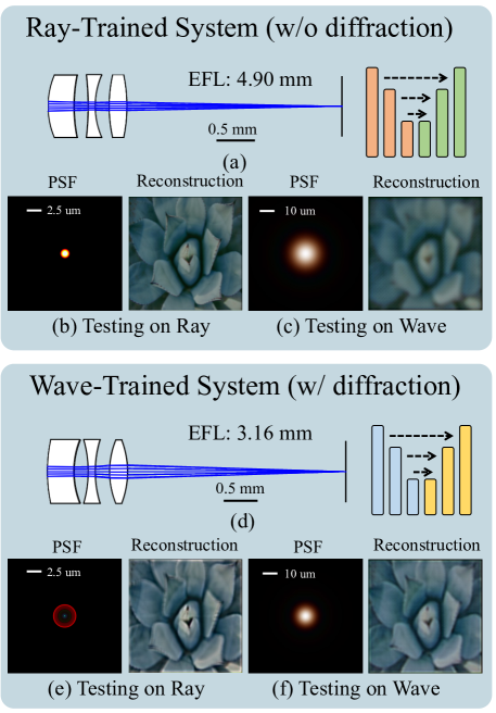
Figure 6: Lens architecture optimized with (a) ray and (d) wave optics. In each system, we visualize its PSF and reconstruction results obtained by using (b)(e) ray and (c)(f) wave optics in testing.

4.3 Demosaicking and Reconstruction

In addition to lens physics, we also incorporate the Bayer filter as follows. We simulate beam propagation from red, green, and blue light channels, compute corresponding measurements in these three wavelengths, and subsequently subsample these measurements using the Bayer filter, resulting in blurred and mosaicked measurements.

We employ a U-Net architecture [23] to recover scene intensities from blurred and mosaicked measurements rendered from the high-resolution DIV2K dataset [1] for training and evaluation. The optimization is guided by a loss function, which comprises a weighted sum of the mean squared error and perceptual loss [35].

Recognizing the significant role of diffraction in small aperture systems, we perform end-to-end optimizations on a lens with a 0.1 mm aperture to examine the dependency of lens structure and reconstruction performance on the chosen physics model. In Fig 6 (a) and (d), we first observe that optimized lens structure highly depends on the physics model chosen during the training phase, with the F-number of the wave-optimized lens being considerably lower than that of the ray-optimized lens. As shown in Fig. 6 (b) and (e), if we only consider ray optics, the optimized lens yields more energy-concentrated PSF than the wave-optimized lens does. However, Fig. 6 (c) and (f) show that once we simulate PSFs in wave optics, the wave-optimized lens performs better in concentrating the energy than the ray-trained lens does.

Fig. 6 (b) and (c) show that although the ray-optimized system is capable of achieving a small geometric spot size, it neglects the blur resulting from wave optics effects. Once the geometric spot size is on the order of the diffraction spot size, the prediction of image sharpness becomes unreliable. When evaluating the system with the more accurate wave model, it encounters degradations on both PSF quality and reconstruction performance. Therefore, ray-trained lens designs are overly optimistic about image quality and downstream algorithm performance. Conversely, as shown in Fig. 6 (e) and (f), the wave-trained system has worse geometric performance (still diffraction-limited) than the ray-trained system, but better overall performance. This is because the lens has converged to a solution with a lower f-number, shown in Fig. 6 (d), thereby improving the diffraction limited resolution. This demonstrates that the choice of physical models in end-to-end optimization can significantly affect the final lens design and algorithm parameters.

To investigate the dependency of lens design solutions on pixel area and aperture radius, we vary these two parameters in end-to-end optimization and present the results in Table 1, where we consistently use wave optics in testing. As observed, when the pixel size is 1 um, using ray optics versus wave optics results in significant divergence in both lens design and reconstruction performance. However, as the pixel size increases, the divergence in lens design and reconstruction performance diminishes. This is because the PSF structures are discretized into fewer pixels, making the structural changes from diffraction less obvious.

Table 1 also presents the reconstruction performance and optimized lens architecture under different aperture radii. As we increase the aperture radius from 0.1 to 0.3 mm, we obtain a smaller mismatch between lens designs and the performance gap caused by different physics models. This is because when the aperture radius is 0.1 mm, the diffraction spot size significantly exceeds the geometric spot size, allowing the system to adjust its structure to optimize the trade-off between aberration and diffraction performance. However, as we increase the aperture size, the system transitions from diffraction-limited to aberration-limited, thus discouraging the system from trading aberration performance for diffraction performance.

Table 2: Classification accuracy on wave optics rendered measurements

Pixel size (um)	Training physics		MF	CL
	Wave	Ray
Aperture radius: 0.1 mm
1	72.0%	48.5%	11.67	0.800
5	72.8%	65.8%	3.177	0.979
10	73.6%	67.7%	0.435	0.999
Aperture radius: 0.3 mm
1	71.2%	63.1%	0.252	0.999
5	73.4%	67.5%	0.104	0.999
10	76.4%	68.7%	0.120	0.999

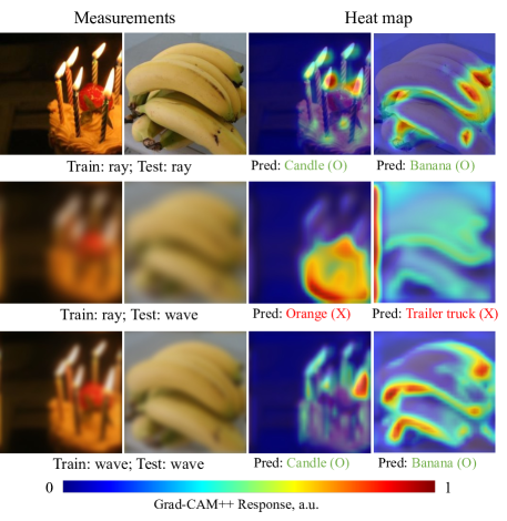
Figure 7: Examples of measurements and associated heat maps generated by GradCAM++.

4.4 Image Classification

To examine the impact of the physics model on semantic information quality in rendering, we conduct end-to-end optimization for image classification. The training dataset consists of 10 image classes from ImageNet [8], with 800 images used for training and 100 images for testing per class. We utilize ResNet18 [12] for class label estimation and employ cross-entropy loss to drive the joint optimization of both the lens and the network.

We perform end-to-end optimization of triplet lenses across different physics models, aperture radii, and pixel sizes, with classification performance consistently evaluated using measurements rendered with wave optics. As summarized in Table 2, for an aperture radius of 0.1 mm, systems optimized by ray optics and wave optics have noticeable differences in F-number and lens architecture. Systems trained without accounting for diffraction but tested with diffraction experience a significant drop in classification accuracy. This performance gap diminishes as pixel size increases, reducing the structural disparity between PSFs. Additionally, with a larger aperture radius of 0.3 mm, the differences in F-number and classification performance between systems optimized using different physics models also become less pronounced, reducing the impact of ignoring diffraction during training.

We also conduct a qualitative analysis of the impact of different physics models used for training lenses with a 0.1 mm aperture radius. Specifically, we employ Grad-CAM++ [5], a technique for network interpretation, to visualize feature extraction during classification. In Fig. 7, we present sample measurements alongside their associated heatmaps. As illustrated in the top row, when the system is optimized using ray optics, the network is trained to capture features from sharp images. Consequently, when tested with ray optics, the network successfully identifies all necessary features for classification. However, as shown in the middle row, introducing diffraction during testing results in blurrier measurements, making the ray-trained network misidentify features and produce erroneous classification results. In contrast, as shown in the bottom row, when diffraction is considered during optimization, the lenses are driven to a lower F-number to mitigate the diffraction blur, and the network is aware of diffraction in feature extraction. This results in less blurry measurements and more accurate feature detection, as demonstrated in the right column. This analysis reaffirms the critical importance of incorporating diffraction in end-to-end optimization.

Table 3: The expected and reference reconstruction performance of system trained by a subset of PSFs (RMSE ($10^{-2}$) / LPIPS)

$N_{T}$	Expected	Reference	$\rightarrow$ (s)	$\leftarrow$ (s)
Singlet Lens
9	1.650 / 0.138	1.961 / 0.226	2.21	7.46
25	1.737 / 0.125	1.798 / 0.176	3.94	17.14
81	1.759 / 0.154	1.793 / 0.159	11.09	52.39
289	1.812 / 0.164	1.819 / 0.164	31.26	176.72
969	1.795 / 0.149	1.795 / 0.149	113.55	679.97
Cooke Triplet Lens
9	2.040 / 0.264	2.041 / 0.265	3.08	10.18
25	1.989 / 0.240	1.990 / 0.241	5.92	23.81
81	1.991 / 0.240	1.992 / 0.241	16.51	72.41
289	1.996 / 0.242	1.997 / 0.243	55.53	253.7
969	1.870 / 0.234	1.870 / 0.234	198.13	975.2
$N_{T}$: The number of PSFs used in approximation and optimization
$\rightarrow$ ($\leftarrow$): Time elapsed in the forward (backward) propagation

4.5 Interpolation

We conduct the following experiments to evaluate the robustness of systems optimized using a subset of PSFs. The system takes 9 to 969 PSFs in optimization, and we measure expected and reference reconstruction performance as follows: Expected performance is evaluated on measurements rendered by the same number of PSFs used in training, and reference performance is evaluated on measurements rendered by 969 PSFs, the maximum achievable under hardware constraints.

As summarized in Table 3, optimizing a Cooke Triplet lens system with just 9 PSFs results in a narrow disparity between expected and reference reconstruction performance. Adding more PSFs further improves both metrics, but they remain closely aligned. In contrast, a singlet lens system optimized with only 9 PSFs tends to yield overly optimistic results, leading to significant degradation in reference performance. This performance gap narrows after increasing the number of PSFs beyond 81. The disparity arises from the limited capacity of the singlet lens to correct off-axis aberrations, making systems trained with isoplanatic assumptions less robust. In comparison, due to a superior aberration control, the Cooke Triplet lens allows robust optimization even with a minimal PSF count. These findings underscore the sampling requirements for optimizing various lens types to balance efficiency and accuracy. Further analysis of the impact of varying PSF quantities is provided in the supplemental materials.

Table 3 also presents the elapsed time for forward and backward propagation in the optimization of the singlet and Cooke Triplet lenses, evaluated on a single image. As shown, backward propagation takes around four times longer than forward propagation, and it takes less time to optimize a singlet lens than Cooke triplet lenses due to lens architecture complexity. Without acceleration via interpolation, backpropagation becomes impractically slow due to extensive computation demands. By reducing the number of PSFs from 969 to 9 in Cooke Triplet lenses, we achieve approximately 60x and 100x speed-ups for forward and backward propagation, respectively. These results indicate that optimizing with a reduced subset of PSFs can yield a generalizable system while significantly reducing computational overhead. On the other hand, due to the weaker isoplanatic properties among PSFs rendered in the singlet lens, to ensure the fidelity of the optimization, the acceleration provided by interpolation is limited.

4.6 Hardware Validation

(a) On-Sim.

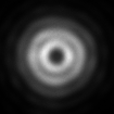
(b) On-Real.

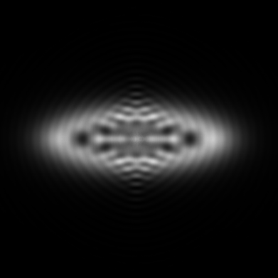
(c) Off-Sim.

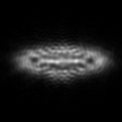
(d) Off-Real.

Figure 8: On-axis and off-axis PSFs generated by our simulator (Sim.) (a)(c) and in real experiments (b)(d).

We validate the physical accuracy of our simulator against real-world hardware implementations. Specifically, we send on-axis and off-axis parallel beams through a plano-convex lens (model 011-1580) onto a sensor (UI-3882LE0M) and generate PSFs. The comparisons between simulated and actual PSFs are displayed in Fig. 8. As observed, when the beams are on-axis, the simulator accurately models the associated diffraction patterns observed in the real PSF. On the other hand, when the beams are off-axis, the simulator accurately captures off-axis aberration and diffraction, yielding similar structures in real and simulated PSFs. These results confirm the simulator’s reliability in capturing wave optics effects across different optical configurations, demonstrating its robustness for modeling diffraction phenomena in practical scenarios.

5 Conclusion

End-to-end optimization exploits the interdependence between optical components and computational algorithms in imaging systems. However, due to insufficient accuracy and efficiency, existing frameworks have not discussed the requirements of modeling wave optics in simulation and the consequences of neglecting it. In this paper, we develop an efficient, accurate, and differentiable wave optics simulator to examine the role of diffraction in end-to-end optimization. The experimental results reveal that modeling light transport with and without wave optics yields different lens configurations and algorithm adaptations to scene reconstruction and classification. When diffraction is not considered in system design, performance degradation can occur under diffraction-limited conditions. These findings highlight the critical importance of physics-aware modeling for high-resolution imaging, especially in systems constrained by diffraction.

Supplementary Material

In this supplemental document, we present additional results of the proposed differentiable wave optics simulator to support our findings.

6 PSFs Rendering

In this section, we demonstrate point spread functions (PSFs) rendered from different incident angles, apertures, and lens configurations.

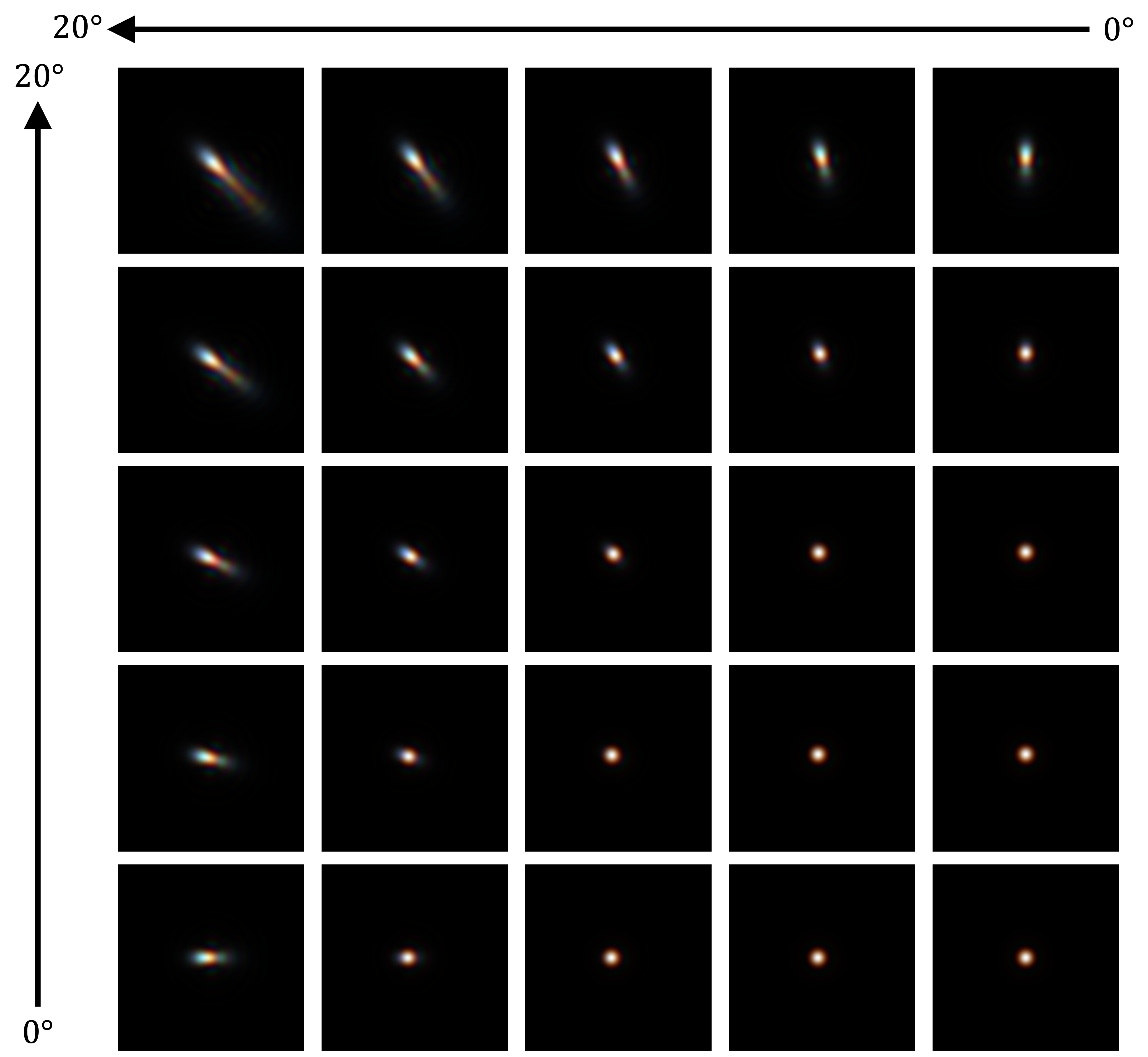
Figure 9: PSFs rendered from a Cooke Triplet lens over the incident angle from 0 to 20 degrees.

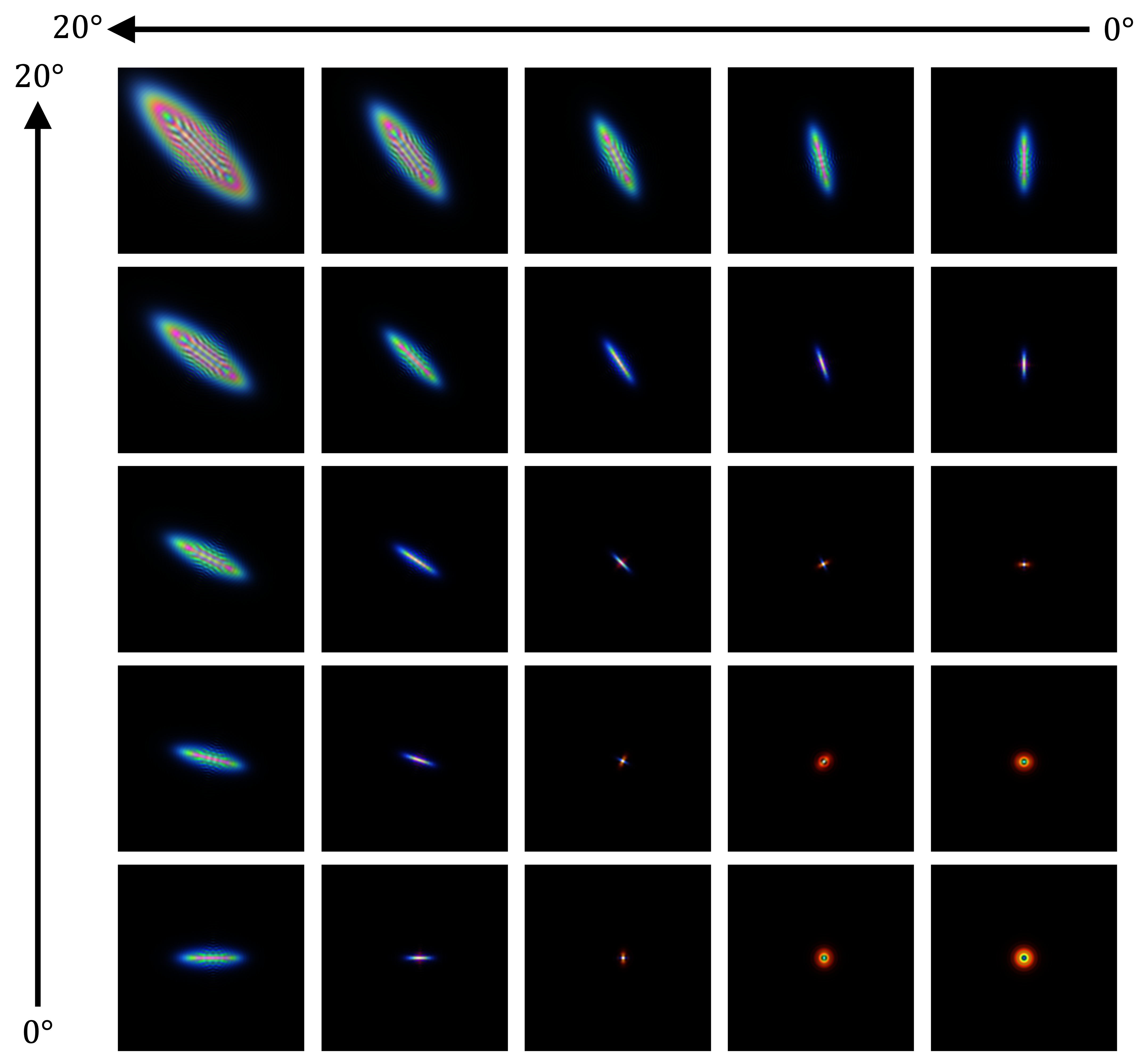
Figure 10: PSFs rendered from a singlet lens over the incident angle from 0 to 20 degrees.

6.1 Off-Axis PSFs

Fig. 9 and 10 illustrate the PSFs rendered across incident angles from 0° to 20° for Cooke Triplet and singlet lenses, respectively. The results demonstrate that our simulator effectively captures variations in PSFs due to changing incident angles. When increasing the incident angle, more astigmatism and coma effects appear on the PSFs. Notably, off-axis aberrations and coma are significantly more pronounced in the PSFs of singlet lens, highlighting its limitations in managing aberrations compared to the Cooke Triplet lenses.

(a) On-axis, in-focus

(b) Off-axis, in-focus

(c) On-axis, out-of-focus

(d) Off-axis, out-of-focus

Figure 11: The phase variations on the wavefront map. All the units in x and y axis are mm.

6.2 Wavefreont Maps

We present wavefront maps for a singlet lens under various conditions in Fig. 11. Fig. 11(a) shows that when sending on-axis rays into an in-focus system, the phase variation across the wavefront map is less than one wavelength. In contrast, Fig. 11(b) shows that off-axis rays introduce significant aberrations, leading to phase shifts spanning over five wavelengths and causing defocus blur in the corresponding PSF. Additionally, we shift the sensor by 0.5 mm to make the system out-of-focus and display PSFs in Fig. 11(c) and 11(d). As observed, the phase variations in the wavefront maps are more pronounced for both on-axis and off-axis beams, highlighting the degree of defocusing. These findings validate our approach of computing the wavefront map at the reference sphere in the exit pupil, which reflects the degree of defocusing.

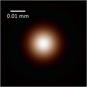
(a) Aperture radius: 0.1 mm, Wave-Rendered

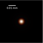
(b) Aperture radius: 0.3 mm, Wave-Rendered

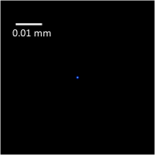
(c) Aperture radius: 0.1 mm, Ray-Rendered

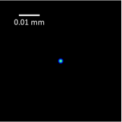
(d) Aperture radius: 0.3 mm, Ray-Rendered

Figure 12: The on-axis PSF rendered aperture radii and physics models.

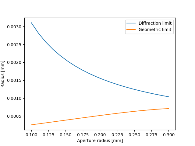
Figure 13: The diffraction and geometric limits of Cooke triplet lens under different aperture radii.

6.3 PSFs Rendered under Different Aperture Sizes

Figure 12 illustrates how increasing the aperture radius reduces the diffraction spot size. When the aperture radius is 0.1 mm, because the system is diffraction limited, the spot size of wave-rendered PSF is much greater than that of ray-rendered PSF. As the aperture radius increases to 0.3 mm, the Airy disk radius decreases and geometric spot size increases, bringing the diffraction and aberration limits closer to each other. These findings confirm our observation that lens divergence depends on aperture size: a larger aperture radius diminishes the differences between PSFs rendered by ray optics and wave optics, indicating reduced sensitivity of system optimization to diffraction effects.

Figure 13 illustrates the change of diffraction and geometric limits with aperture radius. For an aperture radius of 0.1 mm, the diffraction limit significantly exceeds the aberration limit, allowing the system to adjust its configuration to prioritize reducing diffraction effects over aberrations. However, as the aperture radius increases, the diffraction and geometric limits converge, reducing the potential gains from this trade-off. Consequently, systems with larger apertures exhibit diminished flexibility in optimizing between diffraction and aberration performance.

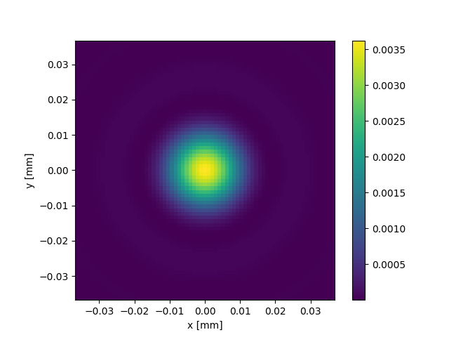
(a) Pixel width: 1um.

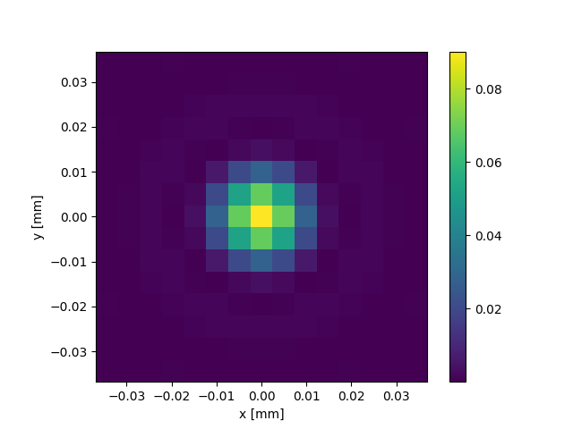
(b) Pixel width: 5 um.

Figure 14: The on-axis PSF rendered with different pixel widths.

Table 4: RMSE ($10^{-2}$) between measurements rendered by 969 PSFs and a subset of PSFs

Lens architecture	9	25	81	289
Singlet	4.41	2.29	1.11	0.385
Triplet	0.174	0.071	0.053	0.052

6.4 PSFs from Different Pixel Sizes

Figure 14 visualizes the PSFs rendered at different pixel sizes. As pixel width increases from 1 to 5 um, the PSF structures become coarser, with diffraction effects appearing less pronounced due to reduced pixel resolution. This observation aligns with our findings that smaller pixel sizes enhance the sensitivity of system optimization to wave optics, underscoring the importance of wave optics modeling for achieving high physical accuracy in imaging systems with high pixel resolutions.

(a) 9 PSFs, singlet.

(b) 25 PSFs, singlet.

(c) 81 PSFs, singlet.

(d) 289 PSFs, singlet.

(e) 969 PSFs, singlet.

(f) 9 PSFs, triplet.

(g) 25 PSFs, triplet.

(h) 81 PSFs, triplet.

(i) 289 PSFs, triplet.

(j) 969 PSFs, triplet.

Figure 15: Measurements rendered by different numbers of PSFs in singlet and triplet lenses.

6.5 Measurements Rendered by Different Number of PSFs

To evaluate how the rendering accuracy depends on the number of PSFs in interpolation, we compare measurements rendered by the measurements rendered a sibset of PSFs with the ones rendered by 969 PSFs in singlet and Cooke triplet lenses rendered, used as the reference. Table 4 summarizes the RMSE between normalized measurements. As observed, in Cooke Triplet lens, using 9 PSFs in interpolation is sufficient to model the reference measurement. However, the singlet lens requires a larger number of PSFs to achieve a negligible RMSE due to its weaker ability to manage distortions and off-axis aberrations.

Figure 15 illustrates example measurements rendered with varying the number of PSFs in interpolation. For measurements rendered from the Cooke triplet lens, the rendering accuracy remain consistent regardless of the number of PSFs used in interpolation. In contrast, the rendering accuracy for the singlet lens strongly depends on the number of PSFs, with noticeable artifacts appearing when interpolation is performed using only 9 PSFs. These results emphasize the importance of selecting an adequate number of PSFs, particularly for lenses with limited aberration control.

7 Lens Architecture

In this section, we present further analysis of the lens architecture optimized under different physics models and the associated PSFs.

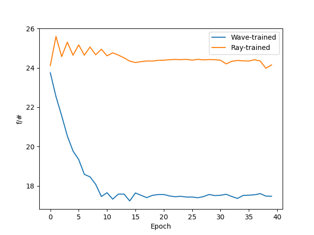
Figure 16: The trend of F-number of triplet lens optimized by different physics models in end-to-end optimization.

7.1 The Analysis of Lens Architecture in End-to-End Optimization

To understand the divergence in optimization paths between the lens system trained by wave and ray optics, we plot the trend of F-number of lenses over successive iterations in Fig. 16. During wave optics-based optimization, the system progressively reduces the F-number to control the PSF spot size. In contrast, under ray optics optimization, where the F-number has little influence on PSF structures, it remains largely unchanged from its initial value throughout the training epochs.

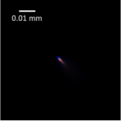
(a) Wave-Optimized, Ray-Tested

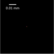
(b) Ray-Optimized, Ray-Tested

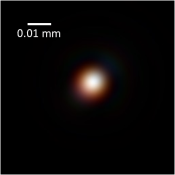
(c) Wave-Optimized, Wave-Tested

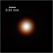
(d) Ray-Optimized, Wave-Tested

Figure 17: The off-axis PSFs of systems optimized in different physics models.

7.2 Off-Axis Performance from Different Lenses

In Fig. 17, we compare off-axis PSFs generated by triplet lenses optimized with wave optics versus ray optics. The ray-optimized lens demonstrates superior control over geometric spot size. However, when wave optics effects are introduced during testing, the wave-optimized lens exhibits a superior ability to mitigate diffraction-related spot size. These results further underscore the importance of accounting for wave optics in end-to-end optimization, highlighting the overly optimistic performance estimates that can arise from neglecting diffraction effects.

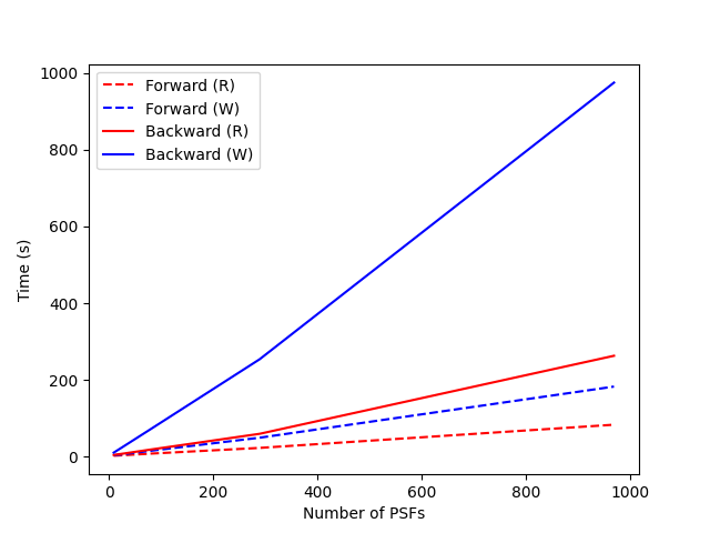
Figure 18: Time elapsed in forward (dash line) and backward (solid line) propagation using wave (W, blue) and ray (R, red) optics.

8 Computation Efficiency

We plot the time elapsed in forward (dash line) and backward (solid line) propagation under different physics models in Fig. 18. As we can see, due to the higher computational costs, wave optics take around twice and four times longer than ray optics in forward and backward propagation, respectively. The analysis demonstrates the need to alleviate the computational costs of driving back-propagation on differentiable wave optics.

9 Free-Form Optics

In addition to normal lens design, we also apply our wave optics model to an inverse rendering experiment on free-form optics [2], where light transportation highly depends on wave optics.

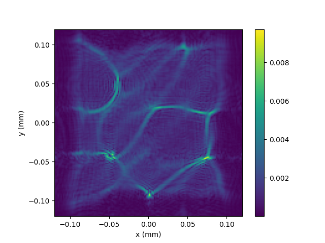
(a) Meshed, On-axis PSF.

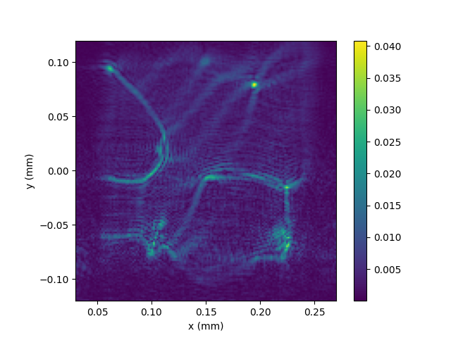
(b) Meshed, Off-axis PSF.

(c) BSpline, On-axis PSF.

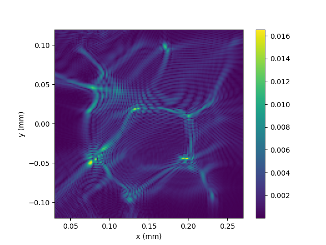
(d) BSpline, Off-axis PSF.

Figure 19: PSFs from free-form optics using different geometric profiles in surface fitting.

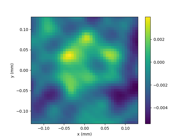
(a) Reference height map.

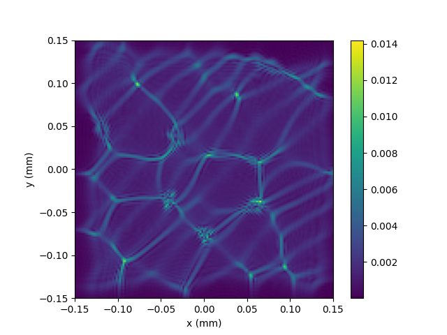
(b) Reference measurements.

(c) Initial height map.

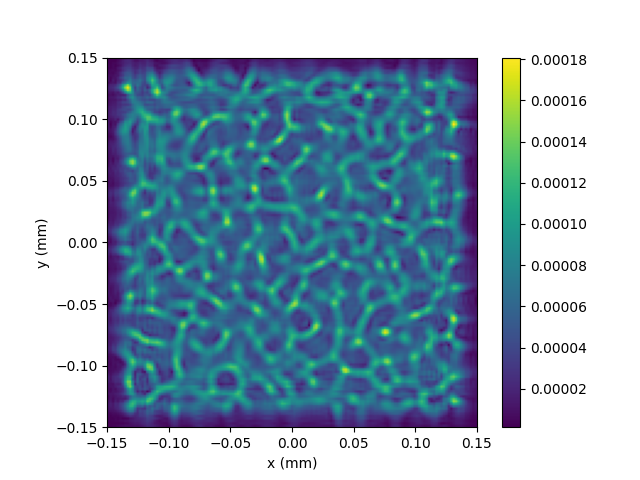
(d) Initial measurements.

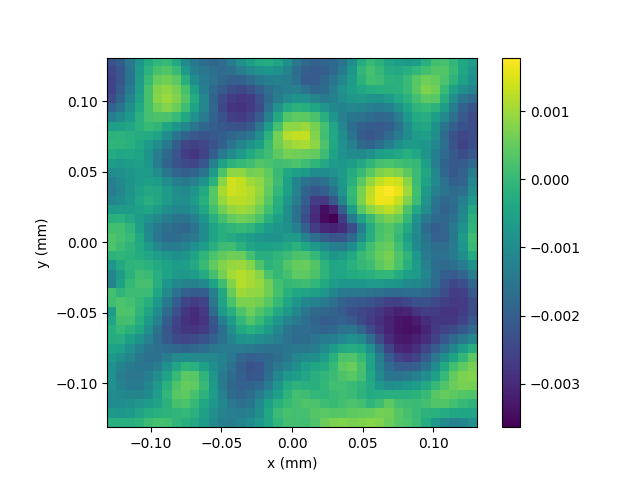
(e) Optimized height map.

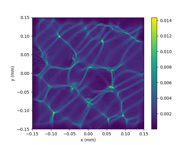
(f) Optimized measurements.

Figure 20: Height maps and associated measurements for reference, initial condition, and optimized results in the experiments. The unit of height maps is mm.

9.1 Measurement Rendering

Provided the discrete height map at given coordinates, we use two geometric profiles, linear meshing and B-spline model, to characterize the surface and render PSFs. For each model, We display on-axis and off-axis measurements generated by our simulator in Fig. 19. As we can see, if we directly mesh the surface with linearly interpolating the heights over the surface, visible artifacts appear, especially for off-axis measurements. On the other hand, as observed in Fig. 19(c) and 19(d), we successfully avoid these artifacts by adopting B-Spline as fitting geometry profile to the height maps. The results demonstrate that the proposed simulator is capable of modeling the structures and off-axis distortions in wave optics propagation in free-form optics.

9.2 Height Map Recovery of Free-Form Optics

We perform differentiable rendering experiments to recover the height map of a free-form optical element. The experiment targets at recovering the reference height map, illustrated in Fig. 20(a), with measurement visualized in Fig. 20(b). Starting from the randomly initialized optics surface, shown in Fig. 20(c), and associated measurements shown in Fig. 20(d), we use the mean squared error between rendered and reference measurement, to drive the optimization of free form optics surface.

Figures 20(e) and 20(f) present the optimized height maps and the corresponding measurement. As observed, the recovered height map closely aligns with the reference, and the rendered measurements accurately replicate the reference measurements. These results demonstrate the versatility and effectiveness of our differentiable wave optics simulator in designing and optimizing non-lens optical systems.

References

- Agustsson and Timofte [2017] Eirikur Agustsson and Radu Timofte. Ntire 2017 challenge on single image super-resolution: Dataset and study. In Proceedings of the IEEE conference on computer vision and pattern recognition workshops, pages 126–135, 2017.
- Antipa et al. [2017] Nick Antipa, Grace Kuo, Reinhard Heckel, Ben Mildenhall, Emrah Bostan, Ren Ng, and Laura Waller. Diffusercam: lensless single-exposure 3d imaging. Optica, 5(1):1–9, 2017.
- Baek et al. [2021] Seung-Hwan Baek, Hayato Ikoma, Daniel S Jeon, Yuqi Li, Wolfgang Heidrich, Gordon Wetzstein, and Min H Kim. Single-shot hyperspectral-depth imaging with learned diffractive optics. In Proceedings of the IEEE/CVF International Conference on Computer Vision, pages 2651–2660, 2021.
- Baktash et al. [2022] Hossein Baktash, Yash Belhe, Matteo Giuseppe Scopelliti, Yi Hua, Aswin C Sankaranarayanan, and Maysamreza Chamanzar. Computational imaging using ultrasonically-sculpted virtual lenses. In 2022 IEEE International Conference on Computational Photography (ICCP), pages 1–12. IEEE, 2022.
- Chattopadhay et al. [2018] Aditya Chattopadhay, Anirban Sarkar, Prantik Howlader, and Vineeth N Balasubramanian. Grad-cam++: Generalized gradient-based visual explanations for deep convolutional networks. In 2018 IEEE winter conference on applications of computer vision (WACV), pages 839–847. IEEE, 2018.
- Chen et al. [2021] Shiqi Chen, Huajun Feng, Dexin Pan, Zhihai Xu, Qi Li, and Yueting Chen. Optical aberrations correction in postprocessing using imaging simulation. ACM Transactions on Graphics (TOG), 40(5):1–15, 2021.
- Côté et al. [2023] Geoffroi Côté, Fahim Mannan, Simon Thibault, Jean-François Lalonde, and Felix Heide. The differentiable lens: Compound lens search over glass surfaces and materials for object detection. In Proceedings of the IEEE/CVF Conference on Computer Vision and Pattern Recognition, pages 20803–20812, 2023.
- Deng et al. [2009] Jia Deng, Wei Dong, Richard Socher, Li-Jia Li, Kai Li, and Li Fei-Fei. Imagenet: A large-scale hierarchical image database. In 2009 IEEE conference on computer vision and pattern recognition, pages 248–255. Ieee, 2009.
- Fontbonne et al. [2022] Alice Fontbonne, Hervé Sauer, and François Goudail. Comparison of methods for end-to-end co-optimization of optical systems and image processing with commercial lens design software. Optics Express, 30(8):13556–13571, 2022.
- Goodman [2005] Joseph W Goodman. Introduction to Fourier optics. Roberts and Company publishers, 2005.
- Halé et al. [2021] Aymeric Halé, Pauline Trouvé-Peloux, and J-B Volatier. End-to-end sensor and neural network design using differential ray tracing. Optics express, 29(21):34748–34761, 2021.
- He et al. [2016] Kaiming He, Xiangyu Zhang, Shaoqing Ren, and Jian Sun. Deep residual learning for image recognition. In Proceedings of the IEEE conference on computer vision and pattern recognition, pages 770–778, 2016.
- He et al. [2023] Tianyue He, Qican Zhang, Chongyang Zhang, Tingdong Kou, and Junfei Shen. Learned digital lens enabled single optics achromatic imaging. Optics Letters, 48(3):831–834, 2023.
- Jenkins and White [1957] Francis Arthur Jenkins and Harvey Elliott White. Fundamentals of optics. Indian Journal of Physics, 25:265–266, 1957.
- Kellman et al. [2019] Michael R Kellman, Emrah Bostan, Nicole A Repina, and Laura Waller. Physics-based learned design: optimized coded-illumination for quantitative phase imaging. IEEE Transactions on Computational Imaging, 5(3):344–353, 2019.
- Kingma [2014] Diederik P Kingma. Adam: A method for stochastic optimization. arXiv preprint arXiv:1412.6980, 2014.
- Li et al. [2021] Zongling Li, Qingyu Hou, Zhipeng Wang, Fanjiao Tan, Jin Liu, and Wei Zhang. End-to-end learned single lens design using fast differentiable ray tracing. Optics Letters, 46(21):5453–5456, 2021.
- Liu et al. [2021] Yuankun Liu, Chongyang Zhang, Tingdong Kou, Yueyang Li, and Junfei Shen. End-to-end computational optics with a singlet lens for large depth-of-field imaging. Optics express, 29(18):28530–28548, 2021.
- Manual [2011] Zemax Manual. Optical design program. 2011.
- Paszke et al. [2017] Adam Paszke, Sam Gross, Soumith Chintala, Gregory Chanan, Edward Yang, Zachary DeVito, Zeming Lin, Alban Desmaison, Luca Antiga, and Adam Lerer. Automatic differentiation in pytorch. 2017.
- Peng et al. [2019] Yifan Peng, Qilin Sun, Xiong Dun, Gordon Wetzstein, Wolfgang Heidrich, and Felix Heide. Learned large field-of-view imaging with thin-plate optics. ACM Trans. Graph., 38(6):219–1, 2019.
- Pidhorskyi et al. [2022] Stanislav Pidhorskyi, Timur Bagautdinov, Shugao Ma, Jason Saragih, Gabriel Schwartz, Yaser Sheikh, and Tomas Simon. Depth of field aware differentiable rendering. ACM Transactions on Graphics (TOG), 41(6):1–18, 2022.
- Ronneberger et al. [2015] Olaf Ronneberger, Philipp Fischer, and Thomas Brox. U-net: Convolutional networks for biomedical image segmentation. In Medical image computing and computer-assisted intervention–MICCAI 2015: 18th international conference, Munich, Germany, October 5-9, 2015, proceedings, part III 18, pages 234–241. Springer, 2015.
- Shannon [1997] Robert R Shannon. The art and science of optical design. Cambridge University Press, 1997.
- Shi et al. [2022] Zheng Shi, Yuval Bahat, Seung-Hwan Baek, Qiang Fu, Hadi Amata, Xiao Li, Praneeth Chakravarthula, Wolfgang Heidrich, and Felix Heide. Seeing through obstructions with diffractive cloaking. ACM Transactions on Graphics (TOG), 41(4):1–15, 2022.
- Sitzmann et al. [2018] Vincent Sitzmann, Steven Diamond, Yifan Peng, Xiong Dun, Stephen Boyd, Wolfgang Heidrich, Felix Heide, and Gordon Wetzstein. End-to-end optimization of optics and image processing for achromatic extended depth of field and super-resolution imaging. ACM Transactions on Graphics (TOG), 37(4):1–13, 2018.
- Sun et al. [2021] Qilin Sun, Congli Wang, Fu Qiang, Dun Xiong, and Heidrich Wolfgang. End-to-end complex lens design with differentiable ray tracing. ACM Trans. Graph, 40(4):1–13, 2021.
- Tan et al. [2021] Shiyu Tan, Yicheng Wu, Shoou-I Yu, and Ashok Veeraraghavan. Codedstereo: Learned phase masks for large depth-of-field stereo. In Proceedings of the IEEE/CVF Conference on Computer Vision and Pattern Recognition, pages 7170–7179, 2021.
- Tseng et al. [2021] Ethan Tseng, Ali Mosleh, Fahim Mannan, Karl St-Arnaud, Avinash Sharma, Yifan Peng, Alexander Braun, Derek Nowrouzezahrai, Jean-Francois Lalonde, and Felix Heide. Differentiable compound optics and processing pipeline optimization for end-to-end camera design. ACM Transactions on Graphics (TOG), 40(2):1–19, 2021.
- Wang et al. [2022] Congli Wang, Ni Chen, and Wolfgang Heidrich. do: A differentiable engine for deep lens design of computational imaging systems. IEEE Transactions on Computational Imaging, 8:905–916, 2022.
- Wei et al. [2023] Haoyu Wei, Xin Liu, Xiang Hao, Edmund Y Lam, and Yifan Peng. Modeling off-axis diffraction with the least-sampling angular spectrum method. Optica, 10(7):959–962, 2023.
- Yang et al. [2023a] Xinge Yang, Qiang Fu, Mohamed Elhoseiny, and Wolfgang Heidrich. Aberration-aware depth-from-focus. IEEE Transactions on Pattern Analysis and Machine Intelligence, 2023a.
- Yang et al. [2023b] Xinge Yang, Qiang Fu, Yunfeng Nie, and Wolfgang Heidrich. Image quality is not all you want: Task-driven lens design for image classification. arXiv preprint arXiv:2305.17185, 2023b.
- Yang et al. [2024] Xinge Yang, Matheus Souza, Kunyi Wang, Praneeth Chakravarthula, Qiang Fu, and Wolfgang Heidrich. End-to-end hybrid refractive-diffractive lens design with differentiable ray-wave model. arXiv preprint arXiv:2406.00834, 2024.
- Zhang et al. [2018] Richard Zhang, Phillip Isola, Alexei A Efros, Eli Shechtman, and Oliver Wang. The unreasonable effectiveness of deep features as a perceptual metric. In Proceedings of the IEEE conference on computer vision and pattern recognition, pages 586–595, 2018.
- Zhang et al. [2023] Rongshuai Zhang, Fanjiao Tan, Qingyu Hou, Zongling Li, Zaiwu Sun, Changjian Yang, and Xiangyang Gao. End-to-end learned single lens design using improved wiener deconvolution. Optics Letters, 48(3):522–525, 2023.