Interpolating amplitudes
Abstract
While the calculation of scattering amplitudes at higher orders in perturbation theory has reached a high degree of maturity, their usage to produce physical predictions within Monte Carlo programs is often hampered by the slow evaluation of the multi-loop amplitudes, especially so for amplitudes calculated numerically. As a remedy, interpolation frameworks have been successfully used in lower dimensions, but for higher-dimensional problems, such as the five dimensions of a phase space, efficient and reliable solutions are sparse.
This work aims to fill this gap by reviewing state-of-the-art interpolation methods, and by assessing their performance for concrete examples drawn from particle physics. Specifically, we investigate interpolation methods based on polynomials, splines, spatially adaptive sparse grids, and neural networks (multilayer perceptron and Lorentz-Equivariant Geometric Algebra Transformer). Our additional aim is to motivate further studies of the interpolation of scattering amplitudes among both physicists and mathematicians.
1 Introduction
Particle physics today demands precision calculations of scattering amplitudes to find hints of physics beyond the Standard Model (BSM) in the data from current colliders. Even more precision is needed to ensure the feasibility of exploiting the much more precise data expected from future colliders.
Impressive progress has been made in the calculation of QCD corrections at next-to-next-to-leading order and beyond to the most important processes at the Large Hadron Collider (LHC) Heinrich:2020ybq ; Gross:2022hyw ; Huston:2023ofk , however most of them are restricted to processes involving relatively few kinematic scales or masses. This is due to the fact that analytic calculations of the required two-loop amplitudes become rapidly unfeasible as the number of external legs and/or particle masses is increasing. For numerical methods the growth in complexity with the number of scales is more tractable. Therefore, the domains of two-loop amplitudes beyond scattering, involving 5 or more kinematic scales, as well as the domains of multi-loop corrections in electro-weak or BSM theories, involving many different masses, are the ones where numerical methods to calculate the virtual amplitudes can prove extremely useful. On the other hand, the usefulness in phenomenological applications is strongly tied to the speed and accuracy at which these amplitudes can be evaluated. In a realistic Monte Carlo evaluation of total or differential cross sections, typically millions of phase-space points need to be evaluated. For this important use case it is unfeasible to embark on a lengthy numerical evaluation of the amplitude for each individual phase-space point.
Therefore, a promising way to make the usage of numerical methods for multi-loop amplitudes more practical is to precompute the values of the amplitudes at some set of points, often a grid, and rely on interpolation to evaluate them at other phase-space points, i.e. for events produced by the Monte Carlo program. However, interpolation for processes needs to be performed on a five-dimensional phase space, which makes it a highly non-trivial task.
The intention of this work is to present a selection of state-of-the-art multidimensional interpolation methods and study their practical usage and performance, having the physics use case in mind. While there is vast mathematical literature on interpolation, the test functions used in mathematics often have different properties than the functions related to loop amplitudes. The purpose of this article is to connect the mathematical literature with the physics use cases that so far were mostly limited to interpolation in dimensions lower than five.
The remaining part of this paper is structured as follows: in Section 2 we give a brief introduction to amplitudes and cross sections. We formulate the interpolation problem and define the error metrics and test functions we use to benchmark the approximation methods. In Sections 3, 4, 5 and 6, four categories of methods are described. Section 3 is about polynomial interpolation, Section 4 about B-splines, Section 5 about sparse grids and Section 6 about machine learning techniques. In these sections, the main results are presented in the form of plots of the approximation error against the amount of training data. We conclude in Section 7 by summarizing the results of the previous sections. Further details on the parametrization of the test functions are given in Appendix A.
2 Setting the stage
2.1 What is an amplitude?
In a proton–proton collider of collision energy , the number of times a reaction
| (1) |
takes place is proportional to the differential cross section of the process pdg24 , which, assuming that the squared masses of partons and are much smaller than , is
| (2) |
where is the scattering amplitude for the process , is the element of the Lorentz-invariant phase space, given in terms of the four-momenta , , and masses as
| (3) |
and is the probability of finding partons and with collision energy in the colliding proton pair, given via the parton distribution functions as
| (4) |
Parton distribution functions themselves are well studied and readily available via Buckley:2014ana . The amplitude is normally calculated within perturbation theory as an expansion in a small coupling parameter, e.g. the strong coupling :
| (5) |
Each subsequent term of this expansion is much harder to calculate than the previous one, so when calculating , one can consider and to be readily available. Tools exist for the automated calculation of up to the next-to-leading order Cascioli:2011va ; Bevilacqua:2011xh ; Alwall:2014hca ; GoSam:2014iqq ; Actis:2016mpe ; beyond that, the calculations are usually custom-made for each process.
The differential cross section depends on the parameters that fully characterize the phase space. These are two for processes, five for , nine for , etc. There is a freedom to choose these parameters; common choices are energy or Mandelstam variables, , and angular variables. In what follows, we denote these parameters as , and choose them such that the physical region of the process is a hypercube: .
The primary use of amplitudes is to calculate cross sections—either the total values over the whole phase space: , or differential over some phase-space partitioning defined either via some observable quantity : , or via a sequence of them, as in e.g. Berger:2019wnu .
2.2 Our goal
Assume that we can calculate most parts of a squared amplitude quickly and precisely, but one part, e.g. a subleading order in , is slow or expensive to evaluate. Let us denote this part as . We aim to approximate by some function , from the knowledge of the values of at some data points : . We are interested in algorithms to choose and to construct such that it is “close enough” to , while requiring as few data points as possible, as to minimize the expensive evaluations of .
2.3 How to define the approximation error?
There are different ways to precisely define what “close enough” means, and no single definition works equally well for all observables and phase-space regions of interest, so a choice of what to prioritize must be made.
In this paper we choose as the probability density of interest, and define the approximation error as the distance between probability densities based on and , measured via the norm:111Here and throughout, we define the -norm as .
| (6) |
The choice of the norm ensures that this quantity is independent of the choice of variables . In statistics, it is known as total variation distance (up to an overall normalization). This distance weighs different phase-space regions proportional to their contribution to the total cross section (via the factor ), and guarantees that for any phase-space subregion , using instead of will result in the error of being no more than . We target of at most 1%.
Note that the precision of the total cross section comes at the expense of precision in tails of differential distributions: for parts of the phase space that do not contribute much to the total cross section, such as the very-high-energy region, only low precision is guaranteed by a bound on . An alternative definition of the error, , would ensure equal relative precision for all bins of any differential distribution, but would come at the expense of the interpolation spending most effort on phase-space regions where only few (or zero) experimental data points can be expected at the LHC. This is the trade-off involved in error target choices; to apply the methods we study, each application would need to choose its own appropriate error measure.
2.4 How to prioritize different phase-space regions?
Summarizing Section 2.3, we approximate , and encode the relative importance of different phase-space regions into . But can we incorporate this importance information to improve the approximation procedure? There are multiple options:
-
1.
Instead of constructing an approximation for directly, we can construct an approximation for , and then set .
-
2.
For methods based on regression, we can choose the data points such that they cluster more in regions where is greater.
-
3.
For adaptive methods, we can approximate , but use the quantity in the adaptivity condition, so that regions where (and not just ) is approximated the worst are refined first.
-
4.
We can find a variable transformation from to that cancels , and interpolate in instead of . In other words, choose with such that , so that .
We know of no general way to construct such transformations in the multidimensional case, but a popular approach is to approximate as its rank-1 decomposition: ; this is the basis of the Vegas integration algorithm Lepage78 . Higher-rank approximations are, of course, also possible.
2.5 The test functions
In the remainder of the article we assess the performance of the most promising interpolation algorithms studied in numerical analysis when applied to the following five test functions.
- Test function :
-
Leading-order (tree-level) amplitude for taken as a 5-dimensional function over the phase space as described in Agarwal:2024jyq . Specifically,
(7) with the phase space parameters set as
(8) (9) The phase space parameters are described in more detail in Appendix A.1. To specify it is possible to use eq. (4) together with one of the well known parton distribution functions, but to be more self-contained, we use the following generic form of :
(10) and set , which approximates computed using the parton distribution functions from Alekhin:2017kpj . The overall proportionality constant is omitted here because it cancels in the error definition of eq. (6).
The amplitude possesses multiple discrete symmetries. For us of immediate interest are the symmetry under (parity invariance), and the symmetry of the swap . These two symmetries are present in all higher order corrections to this amplitude too; the leading order is additionally symmetric under the swap . In terms of the variables , this works out to
(11) (12) (13) As an illustration, slices of the amplitude in – and – space are as follows:
![[Uncaptioned image]](/html/2412.09534/assets/x1.png)
![[Uncaptioned image]](/html/2412.09534/assets/x2.png)
The same slices for the function Test function : are:
![[Uncaptioned image]](/html/2412.09534/assets/x3.png)
![[Uncaptioned image]](/html/2412.09534/assets/x4.png)
- Test function :
-
One-loop amplitude contributing to , taken as a 5-dimensional function. This amplitude has an integrable Coulomb-type singularity at , which needs to be tamed for interpolation to work well. We do this by subtracting the singular behaviour using eq. (2.67) from Beenakker:2002nc , i.e.:
(14) (15) where is a colour operator defined in Beenakker:2002nc and is the velocity of the system, in our variables given by
(16) Both the phase space and are the same as for Test function :. The amplitude possesses two of the symmetries of :
(17) Slices of the amplitude in – and – space are as follows:
![[Uncaptioned image]](/html/2412.09534/assets/x5.png)
![[Uncaptioned image]](/html/2412.09534/assets/x6.png)
The same slices for the function Test function : are:
![[Uncaptioned image]](/html/2412.09534/assets/x7.png)
![[Uncaptioned image]](/html/2412.09534/assets/x8.png)
- Test function :
-
Leading-order (tree-level) amplitude for ,
(18) with the same kinematics and phase space as for Test function :, and chosen via the ansatz of eq. (10) with .
The amplitude possesses the same symmetries as , given in eq. (13).
Slices of the amplitude in – and – space are as follows:
![[Uncaptioned image]](/html/2412.09534/assets/x9.png)
![[Uncaptioned image]](/html/2412.09534/assets/x10.png)
The same slices for the function Test function : are:
![[Uncaptioned image]](/html/2412.09534/assets/x11.png)
![[Uncaptioned image]](/html/2412.09534/assets/x12.png)
- Test function :
-
One-loop amplitude contributing to , taken as a 5-dimensional function, with the Coulomb-type singularity subtracted in the same way as for , i.e.
(19) (20) where is given in eq. (16), and the rest is the same as for Test function :.
The amplitude possesses the same symmetries as and , given in eq. (13).
Slices of the amplitude in – and – space are as follows:
![[Uncaptioned image]](/html/2412.09534/assets/x13.png)
![[Uncaptioned image]](/html/2412.09534/assets/x14.png)
The same slices for the function Test function : are:
![[Uncaptioned image]](/html/2412.09534/assets/x15.png)
![[Uncaptioned image]](/html/2412.09534/assets/x16.png)
- Test function :
-
Leading-order (one-loop) amplitude for , taken as a 2-dimensional function,
(21) with the phase-space parameters set as
(22) (23) the phase-space density being
(24) and chosen via the ansatz of eq. (10), with .
The introduction of as a cutoff is needed because diverges as at and . We choose not to interpolate the region around the divergence, because in practical calculations it should be regulated by infrared subtraction or appropriate kinematic cuts; we only consider the phase-space region where the transverse momentum of the Higgs boson is greater than a cutoff . Then:
(25) We choose corresponding to the lower boundary of the region from eq. (22):
(26) such that at no phase space point passes the cut. This works out to GeV.
The amplitude is symmetric under the swap of the incoming gluons, i.e.
(27) The amplitude (left) and the function Test function : (right) depend on and as follows:
![[Uncaptioned image]](/html/2412.09534/assets/x17.png)
![[Uncaptioned image]](/html/2412.09534/assets/x18.png)
In all cases we use GoSam GoSam:2014iqq to evaluate the amplitudes, and set .
2.6 How to use test function symmetries?
When the test functions are symmetric under discrete transformations, as ours are, there are multiple ways to take advantage of this:
-
1.
Make the interpolant obey the same symmetries by construction.
-
2.
Duplicate symmetric data points, i.e. if , then for each also add to the data set (but still count this as a single evaluation of ).
-
3.
Reduce the interpolation domain, i.e. if , only construct the approximation for , and use the symmetry to obtain the values in .
2.7 How to evaluate the approximation error?
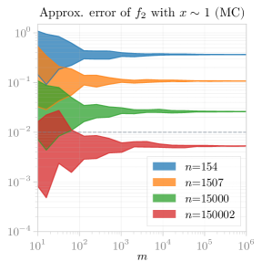
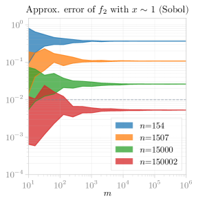
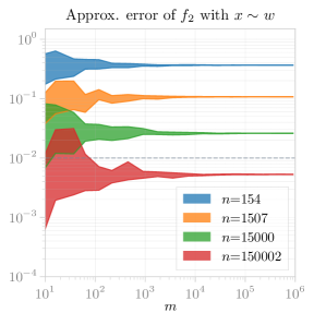
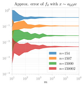
To evaluate eq. (6) we use Monte Carlo integration. It can be formulated based on different kinds of testing samples:
| uniform: | (28) | ||||
| partially unweighted: | (29) | ||||
| leading-order unweighted: | (30) |
The first of these is natural for the selected variables , the second is important because it is independent of the choice of (and can be approximated by e.g. the widely used Rambo sampling technique Kleiss:1985gy ), and the third is important because it is oriented at the approximate probability distribution of physical scattering events, encoded in the leading order amplitude, .
While each sampling method must yield the same result asymptotically, in practice we are interested in using as few testing evaluations as possible. In Figure 1 we compare the error convergence when using the different sampling methods for test function Test function :. Here we see that the error becomes stable for all methods after samples.
Note that a uniform sample can be generated both via Monte Carlo, i.e. randomly, and with a low-discrepancy sequence (such as the Sobol sequence). In Figure 1 we present results for both options, and while sampling from a low-discrepancy sequence gives a more uniform coverage of the parameter space, we see only marginal improvements in the error convergence.
3 Polynomial interpolation
The classic interpolation method is polynomial interpolation Davis63 ; Trefethen19 . In the univariate case is constructed as a polynomial of degree that exactly passes through the interpolation nodes . It can be written in the Lagrange form as
| (31) |
or slightly rewritten in the barycentric form BT04 as:
| (32) |
The barycentric interpolation formula is general enough that with an appropriate choice of the weights , any rational interpolation can be expressed by it; the weights given here, however, correspond to the purely polynomial interpolation of eq. (31).222 Rational interpolation methods, specifically of the non-linear kind, such as the AAA algorithm NST23 , have established themselves as the most efficient one-dimensional interpolation methods, but generalizations to many dimensions are not developed well enough for us to consider them. This is our form of choice for evaluation due to its numerical stability and simplicity.
The error of a polynomial approximation is given by
| (33) |
where is some function of . To minimize this error a priori without the precise knowledge of , one can choose the nodes such that they would minimize over the domain of interest. Doing so is important because a naive choice of equidistant nodes leads to the Runge phenomenon Runge:1901 : the approximation error explodes close to the boundaries, increasingly worse with higher degree of the polynomial. E.g. for 10 nodes on the interval of :
3.1 Chebyshev nodes of the first kind
The product is minimized in the sense of the infinity norm by the Chebyshev nodes of the first kind, which are traditionally given for the domain as
| (34) |
These nodes achieve a uniform over the interval:
3.2 Chebyshev polynomials
Corresponding to these nodes are the Chebyshev polynomials of the first kind:
| (35) |
Specifically, eq. (34) are the zeros of . These polynomials are orthogonal with respect to the weight :
| (36) |
Note that the nodes in eq. (34) are nothing more than equidistant points in , and the corresponding polynomials are simply an even Fourier series in . This is why a transformation from the function values to the coefficients of the decomposition into Chebyshev polynomials ,
| (37) |
is just a Fourier transform (specifically, a discrete cosine transform). Still, for interpolation purposes, the barycentric form of eq. (32) is preferable, since both eq. (37) and the monomial form suffer from rounding errors that prevent their usage for .
3.3 Chebyshev nodes of the second kind
A related set of points that avoids the Runge phenomenon is Chebyshev nodes of the second kind (a.k.a. Chebyshev–Lobatto nodes), traditionally given as
| (38) |
Unlike eq. (34), these points are not located at the zeros of , but rather at the extrema and the end points, with the advantage of being nested: the set of of these is exactly contained in the set of . This comes at the price of not being uniform over the interval:
The property of being nested is important for adaptive interpolation constructions, because larger grids can reuse the results of smaller ones that they contain.
Unfortunately the inclusion of the end points can make this construction impractical for scattering amplitudes. For example, Test function : can not be evaluated at exactly due to loss of numerical precision, and evaluation at is possible, but best avoided, because evaluation time typically grows when approaching this boundary.
3.4 Approximation error scaling
It is known that polynomial interpolation at Chebyshev nodes is logarithmically close to the best polynomial interpolation of the same degree Davis63 . The approximation error itself depends on how smooth the function is Trefethen19 ; Majidian17 ; Xiang18 . If has continuous derivatives and the variation of is bounded, then
| (39) |
If is analytic, and can be analytically continued to an ellipse in the complex plane with focal points at and the sum of semimajor and semiminor axes (a Bernstein ellipse), then
| (40) |
3.5 Gauss nodes
Closely related to Chebyshev nodes, and often considered superior, are Gauss nodes and Gauss–Lobatto nodes, which are the location of zeros and extrema (respectively) of the Legendre polynomials. These have the advantage that a quadrature built on them (Gauss quadrature) is exact for polynomials up to degree , while the same for Chebyshev nodes (Clenshaw–Curtis quadrature) is only exact for polynomials up to degree . In practice, however, the approximation error of both is very close Trefethen11 ; Trefethen21 , and since Gauss nodes are much harder to compute compared to eq. (34), we do not consider them further.
3.6 Multiple dimensions
The simplest generalization to multiple dimensions is to take the set of nodes to be the outer tensor product of the Chebyshev nodes of eq. (34) for each dimension,
| (41) |
with possibly different node count in each dimension, . This corresponds to interpolation via nested application of eq. (32), or via the decomposition
| (42) |
A detailed study of the interpolation error of this construction is presented in GM19 . Roughly speaking, it is similar to eq. (39) and eq. (40), except instead of one must use , which are of the order of , leading to progressively slower convergence as increases. This is known as the curse of dimensionality Bellman .
3.7 Dimensionally adaptive grid
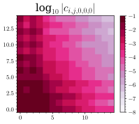
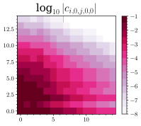
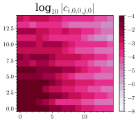
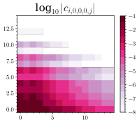
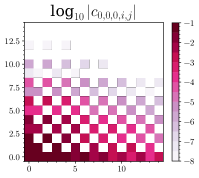
The tensor product construction is fairly rigid in that it allows for no local refinement; only the per-dimension node counts can be tuned. Such tuning is sometimes referred to as dimensional adaptivity, and it can be beneficial. To examine that, let us inspect the coefficients corresponding to Test function :: their two-dimensional slices are presented in Figure 2. From these we can learn that the coefficients decay much faster in the 5th dimension compared to the rest.
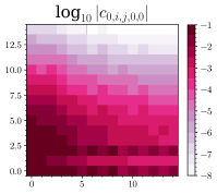
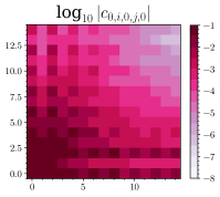
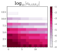
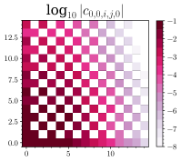

To make use of this insight, let us study Figure 3, where the scaling of is depicted in each dimension. If we want to sample so that coefficients in each direction are close to each other (to prevent oversampling), we would need to maintain the ratio of e.g.
| (43) |
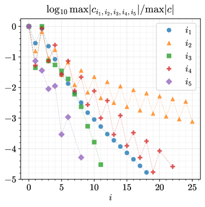
Better results would of course be obtained if instead of a fixed ratio, we would choose the best ratio for each value of ; this, however, can only be done a posteriori.
3.8 Discussion
Polynomial interpolation is a well understood interpolation method. It achieves exponential convergence rates for analytic functions in one dimension, and is easy to evaluate accurately via the barycentric formula. It should be considered a safe and dependable default method.
Its performance in multiple dimensions, however, is held back by the tensor product grid construction, that automatically comes with the curse of dimensionality. It is also sensitive to singularities close to the interpolation space: the closer the singularity, the worse the convergence becomes—this is particularly inconvenient for amplitudes, which are very often not analytic at boundaries. Finally, the method is inflexible: the node sets that do not suffer from the Runge phenomenon are quite rigid, and if an interpolant was constructed with data points, one can not easily add just a few more—the best one can do is to use a nested node set, as in Section 3.3, and roughly double . Similarly, if an interpolant was constructed on a subset of the full phase space, there is no good way to smoothly extend it to the rest of the phase space by adding new data.
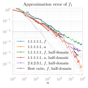
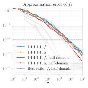
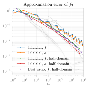
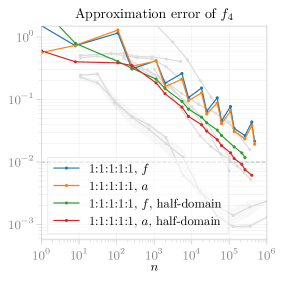
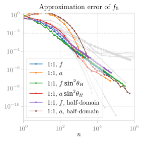
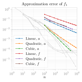
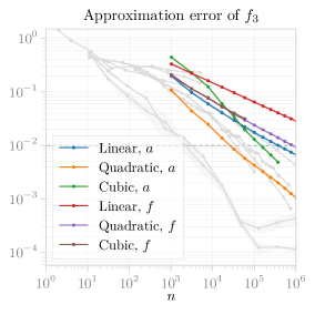
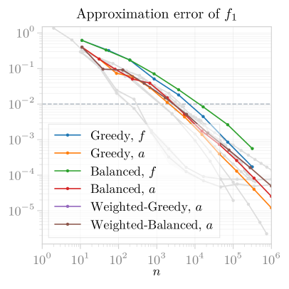
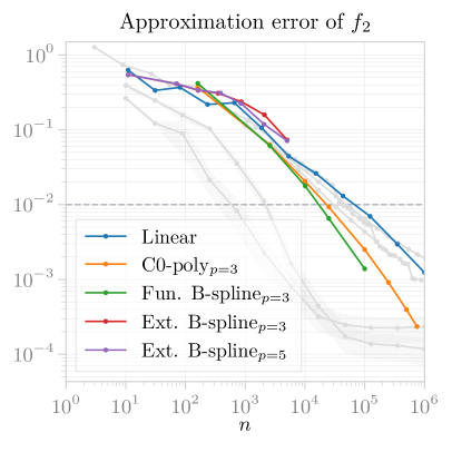
In Figure 4 we present the approximation errors depending on the number of data points , corresponding to different was to use polynomial interpolation in practice: different sampling schemes, symmetry handling options, and ways to include weights. The “” method corresponds to interpolating the amplitude directly, while corresponds to option 1. from Section 2.4. The methods marked with “half-domain” correspond to option 3. from Section 2.6, while the rest correspond to option 2..
Looking at the results, we can conclude:
-
•
Should the interpolant be constructed on or ? Including the weight (i.e. option 1. from Section 2.4) helps a lot for very peaky functions (Test function :), but seems to slightly hinder others. Possible reason is that is not analytic at the boundaries, which polynomial interpolation is sensitive to.
-
•
How should the symmetries be included? Domain reduction (i.e. option 3. from Section 2.6) significantly helps Test function : and Test function :, makes almost no difference for Test function : and Test function :, and slightly hinders Test function :, for which data duplication (i.e. option 2.) is better.
-
•
Does factoring out the known peaky behaviour from the interpolant help? Yes, cancelling the factor from the Test function : interpolant brings a modest, but notable improvement. Subtracting this peak could have been even better though.
-
•
Does dimensional adaptivity help? It only makes a notable improvement for Test function :.
4 B-spline interpolation
An alternative way to prevent the Runge phenomenon in polynomial interpolation is to limit the power of the polynomial, and use a basis of splines. A spline of degree is a times continuously differentiable piecewise polynomial. In this section we use B-splines (basis splines) Schoenberg46 ; Schoenberg67 , which is the standard basis choice for spline interpolation.
B-splines have been applied in engineering applications in the context of the finite element method FEM and in graphics as non-uniform rational B-splines (NURBS) NURBS . B-splines have also been successfully used for interpolating amplitudes in lower-dimensional cases Heinrich_2017 ; Czakon_2024 , which makes this a particularly interesting method for us to compare with. Spline interpolation has also been applied in the context of PDF fits carli2005posterioriinclusionpdfsnlo .
In this section we define the B-spline basis functions and show how to define multidimensional B-spline interpolants on tensor product grids. We then present the resulting approximation errors from using uniform B-splines and finish with a discussion of the obtained performance.
4.1 B-spline basis functions
A B-spline basis function of degree and index is defined recursively through the Cox-de Boor formula Cox72 ; deBoor72 :
| (44) | ||||
where are the coordinates of knots—the locations at which the pieces of the piecewise function meet.
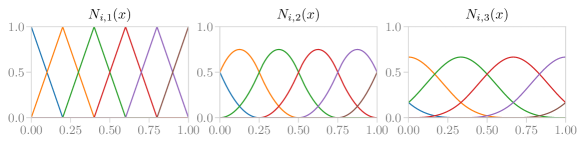
Knots define a knot vector , which is a sequence of non-decreasing numbers . The knot vector should be chosen such that the resulting B-spline basis spans the space of polynomials. This can be checked via the local Marsden identity Lyche2018 . In practice it is fulfilled by either using multiple coinciding knots at the boundaries or by extending the range of the knot sequence HH13 . The most straightforward choice of knot vector is therefore the uniform construction, with auxiliary knots placed outside the interpolation domain. The basis functions resulting from such uniform knot vectors for are shown in Figure 5.
Another common choice is the not-a-knot construction, where knots coincide with data points, except at points, which are omitted. Since in the even degree case this results in an odd number of not-a-knots, this knot vector is better defined for odd degree B-splines. Note that the linear case simplifies to the uniform construction since there not-a-knots in this case.
From eq. (44) it can be seen that the basis functions are non-negative, form a partition of unity, and have local support. Moreover, thanks to the recursive nature of eq. (44), there are efficient algorithms that make B-splines fast to evaluate compared to other spline functions bspline-webpage . This is especially true for B-splines with uniform knot vectors, since the denominators in eq. (44) are constant. In the not-a-knot case the knot distances are not all equal, but can be precomputed in advance.
4.2 B-spline interpolants
A one-dimensional B-spline interpolant is a linear combination of basis functions
| (45) |
where the are interpolation coefficients sometimes referred to as control points. The most straightforward extension to the -dimensional case is through a tensor product construction
| (46) |
To fully constrain a B-spline with basis functions in each direction, interpolation nodes are required. The interpolation nodes can partially be selected freely but need to satisfy the Schoenberg–Whitney conditions, which are degree dependent and state that for each knot there must be at least one data point such that . Moreover, the properties of the basis functions imply that a B-spline interpolant is numerically stable Kermarrec2023 .
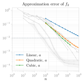
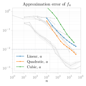
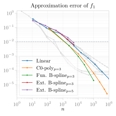
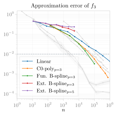
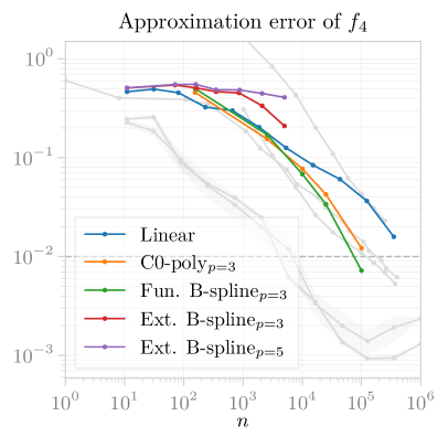
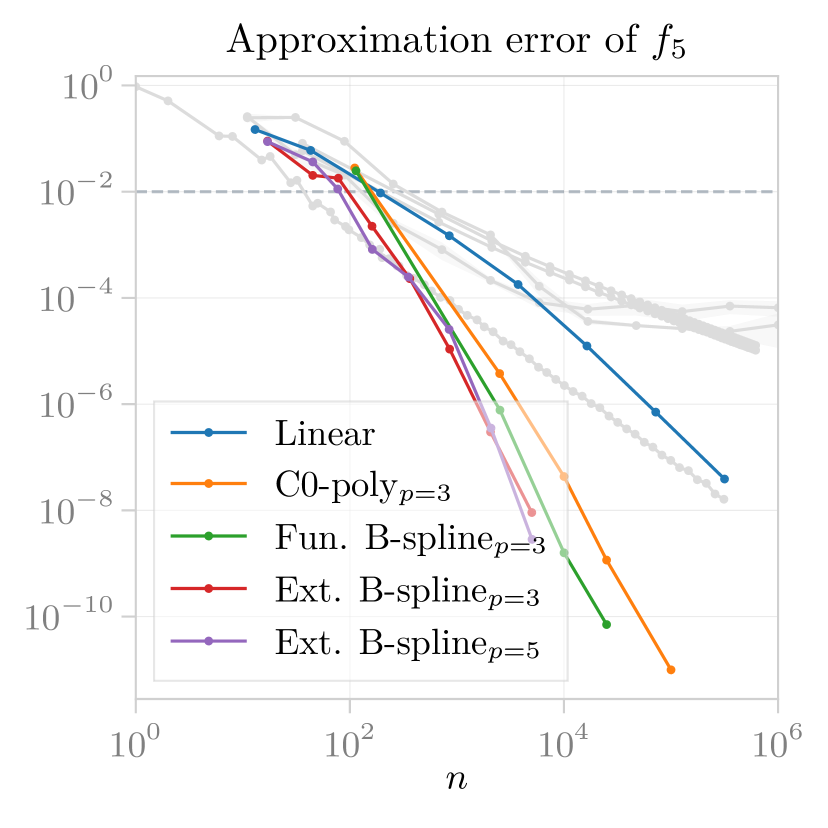
4.3 Discussion
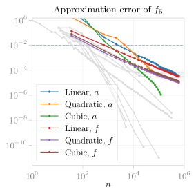
In Figure 6 the performance of B-spline interpolation is compared to the other methods described in this paper. For the 2-dimensional Test function :, percent-level accuracy is obtained with points. For the 5-dimensional test functions, the same accuracy requires points. In most cases a significant performance gain is obtained by using higher degrees than linear, but beyond cubic splines we see no significant improvements. In a few cases, such as for Test function : and Test function :, quadratic splines perform slightly better than cubic splines. The difference between interpolating on the amplitude or directly on the test function is shown for , and . For and it is better to not include the weights during interpolation, while for it is better to include it except for very large .
Besides performance there are additional considerations with B-splines and the tensor product construction in general. One problem is that the construction is made impractical due to the fact that the location of knots and interpolation nodes depend on the total number of points. Consider a situation where a B-spline has been constructed with 1000 data points and the subsequent validation indicates that more points are required to achieve the desired precision target. To then construct a new B-spline with 1100 evaluations, the existing 1000 evaluations would have to be discarded, because the inclusion of additional points would slightly shift the placement of the previous nodes. A special case which avoids this problem is when the number of evaluations is exactly doubled, since in the uniform construction this is equivalent to inserting a new knot and data point between each existing one. In the situation described above, constructing a B-spline using 2000 points would then be the most efficient way to proceed. A more consistent way of avoiding this problem is to combine B-splines with some adaptive strategy. We show in Section 5 how this can be done in the context of sparse grids.
Another potential issue with B-splines based on tensor product constructions, is that function evaluations at the boundary are required. This can be challenging for scattering amplitudes since evaluating at the boundaries can be less precise and more time-consuming than in the bulk of the phase space, as observed in e.g. Agarwal:2024jyq . For such cases, the boundary of the interpolation space can be shifted to a point where the evaluation is reasonable, meaning that the approximation would not cover some parts of the phase space. Alternatively, methods that incorporate extrapolation, such as the modified bases on adaptive sparse grids from Section 5, can be used to alleviate this problem.
5 Sparse grids
The methods described in the previous sections are based on the tensor product construction of eq. (41), which results in a full grid. A sparse grid construction aims to omit points from the full grid that do not significantly contribute to the interpolant, and in this way alleviate the curse of dimensionality. Such constructions were first described by Smolyak Smolyak63 and have since then found use in a wide variety of applications Zenger91 ; sg-survey ; sg-nutshell ; sg-thesis-pflueger ; sg-optimization ; sg-economics ; sg-thesis-Valentin ; sg-thesis-Rehme .
In this section we first introduce sparse grids built on a hierarchical linear basis. Next, we describe how to incorporate spatial adaptivity and upgrade the basis to higher degree polynomials. Finally, we study the impact these constructions have on the approximation quality.
5.1 Classical sparse grids
Sparse grids can be constructed in two main ways, either with the combination technique using a linear combination of full grids GSZ92 , or through a hierarchical decomposition of the approximation space sg-thesis-pflueger . In this section we use the latter approach, since it makes it straightforward to incorporate spatial adaptivity.
First, let us restrict to functions that vanish at the boundaries. In this case, a one-dimensional basis can be constructed with rescaled “hat” functions that are centred around the grid points :
| (47) |
where is the grid level. Since these basis functions have local support, it is possible to define hierarchical subspaces through the hierarchical index sets by
| (48) |
The function space of one-dimensional interpolants is then defined as the direct sum of all subspaces up to a maximum grid level
| (49) |
The extension to the multivariate case is via a tensor product construction
| (50) |
with multi-indices ,
and -dimensional grid points
.
Similarly to the one-dimensional case, the hierarchical subspaces
are defined to be
| (51) |
A multidimensional full-grid function space can now be naively constructed with the direct sum
| (52) |
where . The mechanism of the sparse grid is to instead limit the selection of subspaces according to
| (53) |
where . This avoids including basis functions that are highly refined in all directions simultaneously, which is what causes the number of grid points to explode in high dimensional cases.
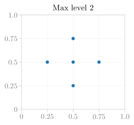
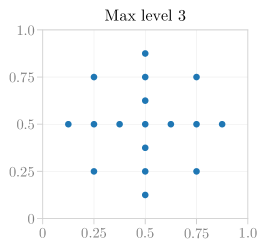
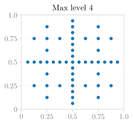
Figure 7 shows nodes of the resulting two-dimensional sparse grids for . Table 1 shows the difference in the number of grid points between sparse and full constructions, for dimensions 2 and 5. Of course, omitting grid points can never increase the approximation quality, but the aim is to achieve a close approximation quality, while omitting most points. For sufficiently smooth functions, it is known that the asymptotic accuracy of a full grid interpolant scales with the mesh-width as , while for a sparse grid it decreases only by a logarithmic factor to (see sg-thesis-pflueger ).
| Grid type | \ | 2 | 4 | 6 | 8 | 10 |
|---|---|---|---|---|---|---|
| Full | 25 | 289 | 4225 | |||
| 3125 | ||||||
| Sparse | 5 | 49 | 321 | 4097 | ||
| 11 | 315 | 5503 |
5.2 Boundary treatment
Since the basis functions of eq. (47) do not have support at the grid boundaries, we can, so far, only handle target functions that vanish at the boundary. There are two main ways to incorporate boundary support into sparse grids. One possibility is to add boundary points to the grid sg-thesis-pflueger , but for even moderately high dimension this causes the number of points to increase significantly, and defeats the main purpose of the sparse construction. The other option is to use so-called modified basis functions sg-thesis-pflueger that linearly extrapolate from the outermost grid points:
| (54) |
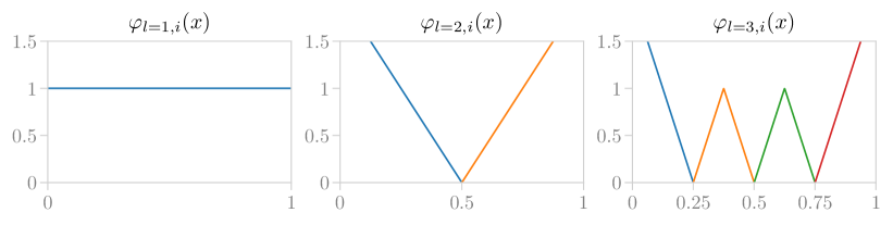
Figure 8 shows the modified linear basis for . It is apparent that sparse grids are best suited for functions whose boundary behaviour is less important than that in the bulk to the overall structure. The interpolant is constructed as a linear combination of basis functions in according to
| (55) |
where the interpolation coefficients are referred to as hierarchical surpluses since at each level they correct the interpolant from the previous level to the target function. They are thus also a measure of the absolute error at each level in each direction, which makes the interpolant well suited for local adaptivity. The basis functions are constructed from either eq. (47) or eq. (54) depending on if the target function vanishes at the boundary or not. The process of determining the coefficients is known as hierarchization. This can in principle be done in the same way as for any interpolation method; construct and solve a linear system of equations where the interpolant is demanded to reproduce the target function at each interpolation node. A more efficient way, however, is available for bases satisfying the fundamental property:
| (56) |
In this case the coefficients can be calculated on the fly: the grid is initialized by normalizing the first coefficient to the central value ; points are then added, one at a time, and the coefficients are defined as the corrections
| (57) |
where is the current approximation with the already added points and is the true function value.
5.3 Spatially adaptive sparse grids
While the classical sparse grid construction uses significantly fewer points than a full grid, it is completely blind to how the target function varies across the parameter space. In many high dimensional problems, it is typical that some regions are more important than others. This information is exploited by spatially adaptive sparse grids, where the grid points that contribute most to the interpolant are refined first (see sg-pflueger-spatially ; sg-thesis-pflueger ). Refining a grid point means adding all its neighbouring points at one level lower to the grid.
Determining which points are more important relies on some heuristic criterion. A common strategy is to use the surplus criterion, where the point with the largest hierarchical surplus is refined first. This is the greedy strategy. Its disadvantage is that it might get stuck refining small regions of the parameter space. To avoid this, in sg-thesis-pflueger it is proposed to weigh the surplus criterion by the volume of the support of the corresponding basis function, , resulting in the balanced strategy.
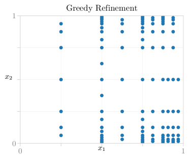
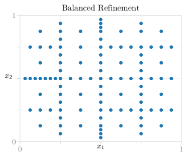
Figure 9 shows the difference between greedy and balanced refinement on a two-dimensional grid. We find that greedy refinement might perform slightly better for our error metric if the structure of the target function is simple enough, while balanced refinement is significantly more reliable for more complicated target functions.
5.4 Higher degree basis functions
The one-dimensional basis of rescaled hat functions in eq. (47) is straightforward to implement and avoids the Runge phenomenon due to its piecewise nature. The drawback is that the linear approximations come with low interpolation performance, as we have previously observed in Section 4.
There are many ways to make the extension to higher polynomial degrees. Here we differentiate between two types of basis functions: those that fulfil the fundamental property eq. (56) and those that do not.
Fundamental basis functions allow for fast hierarchization and make it easy to construct efficient evaluation algorithms. In addition to the linear basis from Section 5.1 we test the more general polynomial piecewise functions (C0-elements) Bungartz1995HigherOF ; sg-thesis-pflueger , as well as fundamental B-splines sg-thesis-Valentin . For these benchmarks we make use of the sparse grid toolbox SG++ sg-thesis-pflueger , where both of these basis functions are already implemented. Beyond fundamental basis functions we also investigate extended not-a-knot B-splines as described in extended-nak-sg-bsplines ; sg-thesis-Rehme .
C0 elements
Higher degree polynomials can be defined on the hierarchical structure by using grid points on upper levels as the polynomial nodes Bungartz1995HigherOF ; sg-thesis-pflueger . This implies the maximum degree is bounded by the maximum grid level. For sparse grids without boundaries the relation is . This can be seen already for the linear case in Figure 8, since on levels 1 and 2 the basis functions are constant and linear respectively. The drawback of this extension is that despite the higher degree, the smoothness is not increased and the interpolant will only be continuous. For this reason these basis functions are usually referred to as C0 elements.
Fundamental B-splines
The fundamental B-spline basis is constructed with the aim of fulfilling the fundamental property of eq. (56), while preserving useful properties of B-splines, for example smoothness. The construction is introduced in sg-thesis-Valentin , and it works by applying a translation-invariant fundamental transformation to the hierarchical B-spline basis. Besides fulfilling the fundamental property, this transformation preserves the translational invariance of B-splines which improves performance during evaluation. The modified basis that extrapolates toward the boundaries is defined similarly to the linear case. We refer to sg-thesis-Valentin for more details on the derivation. For both this and the C0 elements, the implementations in SG++ are used for the benchmarks.
Extended not-a-knot B-splines
In this section we summarize the main equations and statements on extended not-a-knot B-splines presented in extended-nak-sg-bsplines ; sg-thesis-Rehme . The extension mechanism ensures that polynomials are interpolated exactly, which in many cases increases the quality of interpolation. The basis consists of extended not-a-knot B-splines on lower levels, and Lagrange polynomials on upper levels where there are too few points for the B-spline to be defined. A basis function of odd degree , level and index is defined as
| (58) |
where , and are extension coefficients that only depend on the degree. For these coefficients are listed in Table 2.
The are not-a-knot B-splines (see Section 4) and are regular Lagrange polynomials defined with a uniform knot vector as
| (59) |
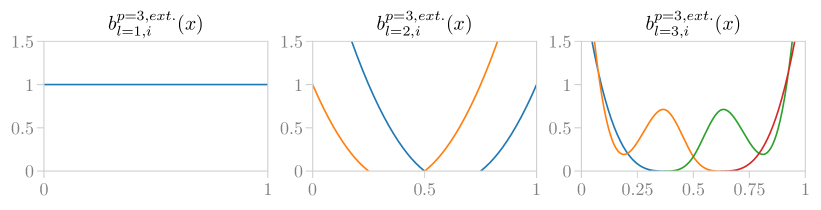
The index set defines the extension of the B-spline. It determines to which interior basis functions the boundary basis functions are added. An interior basis function of index includes the boundary basis function if is among the first or last interior indices. Formally the index set is defined as , where and (see extended-nak-sg-bsplines ). The basis functions described by eq. (58) are shown in Figure 10 for the cubic case. The linear case simplifies to the linear hat-basis described in Section 5.1.
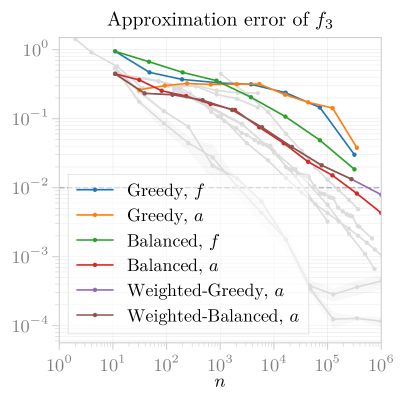
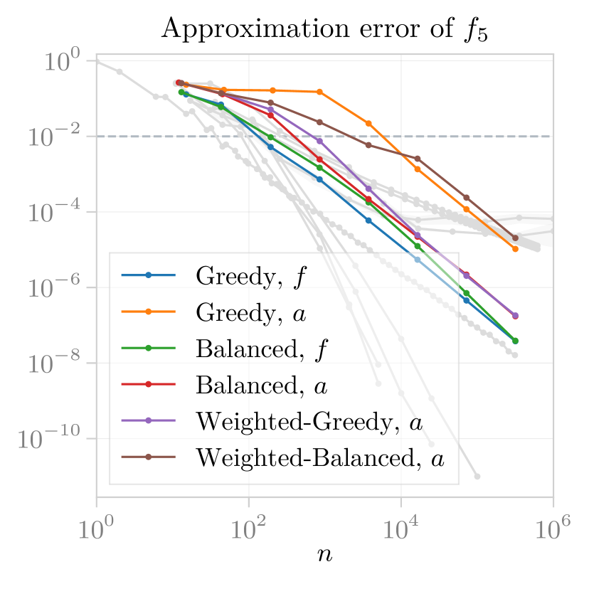
5.5 Discussion
In Figure 12 we compare the approximation error from spatially adaptive sparse grids, constructed with balanced refinement, against the other methods described in this paper. A comparison between different refinement criteria is given in Figure 11 for test functions , and , using the modified linear basis. In some cases the greedy construction is slightly better, but for example the results for Test function : demonstrate the danger of this refinement strategy. The balanced construction results in a much smaller approximation error, which hints at the greedy algorithm getting stuck refining local structures. In practice, it is difficult to predict when refining greedily is better, and in such cases the advantage seems to not be very significant. Moreover, greedy refinement is not very robust against numerical artefacts and noise in the training data. For these reasons we prefer to use some form of balanced refinement, since this is much safer in practice.
We also try to weigh the refinement criterion by the phase-space weight from eq. (29). For Test function : and Test function : this results in a more uniform target function, and the resulting sparse grid becomes similar to the balanced construction without weighting. We therefore see only minor differences in the results from balanced and weighted refinement.
For other basis choices we see significant improvements for all test functions when increasing the degree with the piecewise polynomial and fundamental B-spline bases. With the extended not-a-knot B-splines we see an even better improvement for Test function :, but for Test function :–Test function : the performance is at best similar to the linear case. In particular for Test function : and Test function : the cubic and quintic cases converge very poorly. This result is unexpected since these bases have been applied to high-dimensional test functions with good results in extended-nak-sg-bsplines . We reproduce those benchmarks with our implementation and also cross-check the new results for our test functions with SG++.
The improvements of the spatially adaptive sparse grids over the non-adaptive full grid methods at low amounts of training data are modest. We see in each test function that the scaling is better, however, and that at high amounts of training data the improvements are more significant.
Taking interpolation performance aside, a major advantage of spatially adaptive sparse grids is flexibility. Since it is difficult to predict how much training data is required to reach a certain precision target for an unknown function, it is likely that training data needs to be added iteratively. As is discussed in Section 3 and Section 4, non-adaptive methods are very limited in this regard. A spatially adaptive sparse grid on the other hand is able to add one point at a time, making it possible to validate during construction and in principle stop at exactly the required number of points. If a non-adaptive method is used to reconstruct an unknown function, we are likely to overshoot the required number of points, making the effective number of function evaluations higher than what is represented by these results. The results for the non-adaptive methods at a given training size are therefore the best case scenario, while the sparse grid results are close to what one obtains in practice.
6 Machine Learning Techniques
Machine learning techniques represent a very promising tool for amplitude interpolation Aylett-Bullock:2021hmo ; Maitre:2021uaa ; Badger:2022hwf ; Maitre:2023dqz ; Spinner:2024hjm ; lgatr . These techniques leverage the power of neural networks, approximator functions that are structured as a sequence of operations dependent on learnable parameters. Neural networks can be optimized to approximate any function of a set of inputs to arbitrary precision—given sufficient time and data. This is accomplished by minimizing the loss function, which characterizes how close the neural network results are to the desired ones. The optimization of neural network parameters is performed by evaluating the loss function on data subsets or batches and performing gradient descent to minimize the objective in an iterative way. In our case, neural network trainings are framed as regression tasks, where the output of the network is trained to match a target given an input.
The main advantage that this approach puts forward for the interpolation problem is its versatility. Neural networks by default introduce a minimal bias in the interpolants they can represent, so they can easily adapt to a wide variety of target distributions. Additionally, networks are not limited to a single training or dataset for their optimization. This makes them a prime tool for adaptive interpolation, since after an initial training their evaluated shortcomings can be used as a guideline for optimization through subsequent retrainings.
However, neural network based interpolation techniques face a challenge in precision as function complexity grows. Namely, the performance of neural networks steadily decreases with increased particle multiplicity Badger:2022hwf and the inclusion of beyond tree-level contributions Maitre:2023dqz . One way to partially mitigate this issue is to incorporate prior knowledge about the amplitude symmetries into the learning task. In our case, we focus on the Lorentz symmetry and work with architectures that are aware of the Lorentz invariance of the amplitudes. This feature is also present in all other interpolation methods discussed in this paper, but there are several ways to implement it on neural networks. We explore two ways of enforcing Lorentz invariance. On the one hand, we train a multilayer perceptron (MLP) rosenblatt1958perceptron ; rumelhart1986learning by feeding it only Lorentz invariant inputs. On the other hand, we use the Lorentz-Equivariant Geometric Algebra Transformer (L-GATr) Spinner:2024hjm ; lgatr , a neural network whose operations are constrained to be equivariant (or covariant) with respect to Lorentz transformations.
To approximate our test functions, we train the networks on as functions of the phase-space points using a mean squared error (MSE) loss. We generate the training data points uniformly over the phase space, using a low-discrepancy Sobol sequence. For the testing data points, we use the leading-order-unweighted sampling described in eq. (30). Additionally, we also build an extra dataset from unweighted samples for validation, a routine checkup that is performed regularly during training to prevent overfitting and select the best performing model constructed during training. The validation set size is always 10% of that of the training dataset until it reaches a size of 4000 points; after that it remains constant for larger training sets.
Targets for tree-level processes are preprocessed with a logarithmic standardisation:
| (60) |
where and are the mean and standard deviation of the amplitude logarithm distributions over the whole dataset. When dealing with Test function : and Test function :, this preprocessing is not valid, because takes negative values. We circumvent this issue by reflecting the amplitude distribution with respect to its maximum value, and then applying the logarithmic standardisation.
As for the inputs, all networks are trained on functions of the four-momenta of the sampled points. We derive the four-momenta for each point from their original parametrization presented in eq. (8) and eq. (22). When applying this mapping for Test function :–Test function :, we prepare the inputs so that the angle lies only in the range , which allows all neural networks to take advantage of the parity symmetry of these functions.
All networks are trained for steps with a batch size of 256, the Adam optimizer kingma2017adam and a Cosine Annealing scheduler DBLP:journals/corr/LoshchilovH16a with a maximum learning rate of when training for the test functions and for the test function. Due to instabilities during training, we refrain from applying early stopping and we perform validation checks every 300 iterations.
6.1 MLP
We use an MLP as the first baseline for this task. The MLP is built as a simple fully connected neural network with GELU activation functions hendrycks2023gaussianerrorlinearunits . The inputs for the network are pairwise momentum invariants . Alternative input choices have been tested, including the phase space parameters introduced in eq. (8) and eq. (22), yielding worse results.
The MLP architecture consists of 5 hidden layers with 512 hidden channels each, amounting to learnable parameters. This configuration is chosen as a result of a scan, as the one that performed the best for data points. The inputs are preprocessed by taking their logarithms and performing standardization as in eq. (60).
6.2 L-GATr
Equivariant neural networks constitute a very attractive option for any problem where symmetries are well defined Gong:2022lye ; Ruhe:2023rqc ; Bogatskiy:2023nnw ; Spinner:2024hjm ; lgatr . These networks respect the spacetime symmetry properties of the data in every operation they perform. They do so by imposing the equivariance condition, defined as
| (61) |
where is a network input, is a network operation and is a Lorentz transformation. By restricting the action of the network to equivariant maps, it does not need to learn the symmetry properties of the data during training and its range of operations gets reduced to only those allowed by the symmetry. This makes equivariant networks very efficient to train and capable of reaching high performance with low amounts of training data.
L-GATr is a neural network architecture that achieves equivariance by working in the spacetime geometric algebra representation hestenes1966space . A geometric algebra is generally defined as an extension of a vector space with an extra composition law: the geometric product. Given two vectors and , their geometric product can be expressed as the sum of a symmetric and an antisymmetric term
| (62) |
where the first term can be identified as the usual vector inner product and the second term represents a new operation called the outer product. The outer product allows for the combination of vectors to build higher-order geometric objects. In this particular case, is a bivector, which represents an element of the plane defined by the directions of and .
The spacetime algebra can be built by introducing the geometric product on the Minkowski vector space . The geometric product in this space is fully specified by demanding that the basis elements of the vector space satisfy the following anti-commutation relation:
| (63) |
This inner product establishes that the vectors in the context of the spacetime algebra have the same properties as the gamma matrices from the Dirac algebra. Both algebras are very tightly connected, with the Dirac algebra representing a complexification of the spacetime algebra.
With this notion in mind, we can now cover all unique objects in the spacetime algebra by taking antisymmetric products of the gamma matrices. A generic object of the algebra is called a multivector, and it can be expressed as
| (64) |
In this expression, the components of the multivector are divided in grades, defined by the number of gamma matrix indices that are needed to express them. Namely, constitutes the scalar grade, the vector grade, the geometric bilinear grade, the axial vector grade, and the pseudoscalar grade.
Apart from its extended representation power, the spacetime algebra offers a clear way to define equivariant transformations with respect to the Lorentz group on a wide range of geometric objects in Minkowski space. The main consideration is that Lorentz transformations on algebra elements act separately on each grade brehmer2023geometric ; Spinner:2024hjm . As a consequence, any equivariant map must transform all components of a single grade in the same manner and allow for different grades to transform independently.
This guideline allows for an easy adaptation of standard neural network layers to equivariant operations in the algebra. In the case of L-GATr, this adaptation is performed on a transformer backbone. Transformers vaswani2017attention are ideal architectures to deal with datasets organized as sets of particles, since the attention mechanism can be leveraged to capture correlations between them in a very accurate way. L-GATr is built with equivariant versions of linear, attention, normalization and activation layers vaswani2017attention ; xiong2020layer . It also includes a new layer MLPBlock featuring the geometric product to further increase the expressivity of the network. Its layer structure is
| (65) |
All of these layers are redefined to operate on multivectors and restricted to act on algebra grades independently to ensure equivariance. Further details for each of the layers are provided in Refs. Spinner:2024hjm ; lgatr .
Through this procedure, we build knowledge about the Lorentz symmetry into the architecture, but it can also be used to enforce awareness of the discrete symmetries described in Section 2.6 besides the parity invariance present in Test function :–Test function :. Being a transformer, L-GATr handles individual particle inputs independently and can enforce any exchange symmetry on individual particles. This is performed in practice by including common scalar labels to every set of particles that leave the amplitude invariant under permutation.
To operate with L-GATr, we need to embed inputs into the geometric algebra representation and undo said embedding once we obtain the outputs. For the interpolation problem, inputs always consist of particle 4-momenta , which can be embedded into multivectors as
| (66) |
Each particle is embedded to a different multivector, resulting in the inputs being organized as sets of particles or tokens. Each token also incorporates a distinct scalar label as part of the inputs. The value for these labels is selected according to the permutation invariance pattern of each process we study. This ensures that L-GATr also respects any instance of particle exchange symmetry. The token labels are not part of the multivectors, they are fed to the network as separate scalar inputs. Multivectors and scalars traverse the network through parallel tracks, mixing with each other only at the linear layers.
As for the outputs, we make use of a global token, which is introduced as an extra empty particle entry. This extra token holds no meaning at the input level, but at the output level its scalar component represents the estimator for the target amplitude. As for the inputs, in L-GATr we divide them by the standard deviation over each of the particle momenta to prevent violating equivariance.
Our L-GATr build consists of a model with 8 attention blocks, 64 multivector channels, 32 scalar channels and 8 attention heads, resulting in learnable parameters.
6.3 Discussion
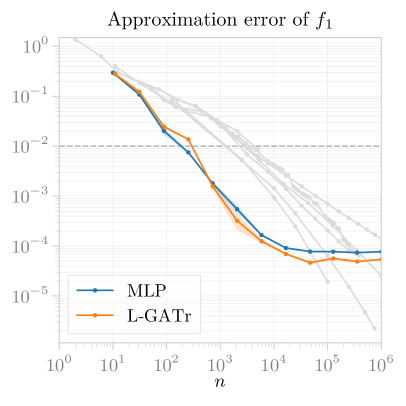
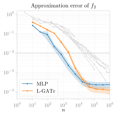
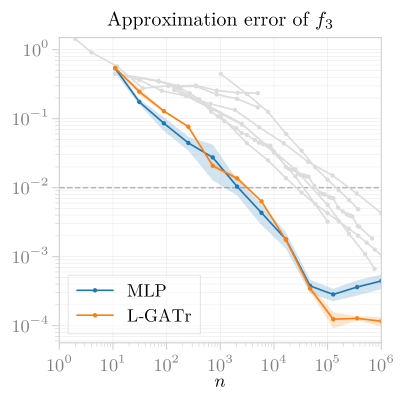
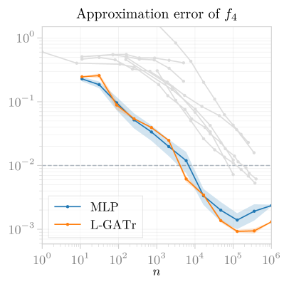
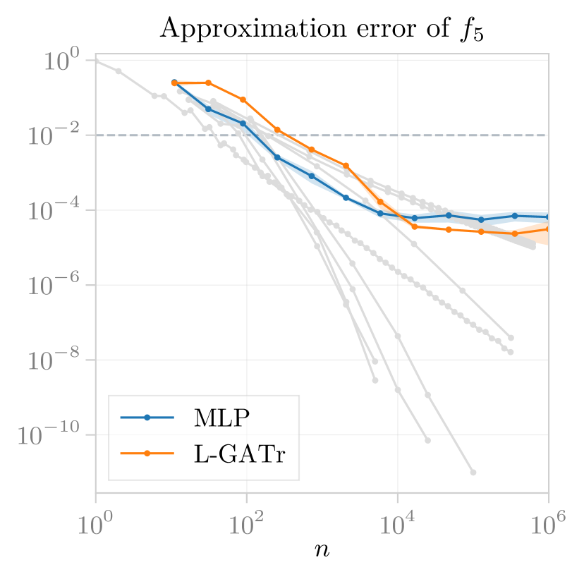
We show the results from both the MLP and L-GATr networks in Figure 13. Both networks manage to clear the percent-level target accuracy on all test functions with a low amount of training points. Comparing our two architectures, the MLP is the best performer with very small training datasets, whereas L-GATr always takes over in the large training dataset limit. From this pattern we can infer that the MLP is slightly more effective at modelling the amplitude distributions in low data regimes, whereas L-GATr becomes better with more training data thanks to its larger capacity. We also observe a general slowdown in improvement for all networks as we increase the training data.
Comparing with other methods, machine learning algorithms surpass all other interpolation methods in the low data regime for all 5-dimensional test functions, and they are only overtaken in the large data regime. Their improvement with respect to other approaches is the biggest in the case of the higher order correction functions and , signalling their potential utility for the interpolation of more complex multi-loop amplitudes.
The only front where neural networks underperform is in the case of the test function. This is the only 2-dimensional function we test, and seeing less benefits from neural networks in lower dimensions should not be surprising.
Another important result that we obtain from this study is that we have the ability to train our neural networks on uniform samples and evaluate them on unweighted samples. If we instead train and evaluate neural networks on datasets produced with a single sampling method we observe only a marginal improvement over the results presented in Figure 13. This is very advantageous for our problem, since that means that we can train our algorithms on datasets produced by naive sampling methods and then evaluate them on physically motivated distributions without a significant performance degradation.
Finally, it is possible to modify the training datasets dynamically to focus on those regions in the target space that are poorly estimated in the initial stages of the training. Such adaptive strategies are hard to balance in practice, since they involve extensive hyperparameter optimization and they are substantially slower than ordinary trainings. For these reasons, we refrain from trying them out in this paper.
7 Conclusions
We have presented a detailed investigation of several frameworks to interpolate multi-dimensional functions, focusing on scattering amplitudes depending on a number of phase space variables. We have used amplitudes related to production (5-dimensional phase space, test functions Test function :–Test function :) and Higgs+jet production (2-dimensional phase space, test function Test function :) at the LHC as test functions, and applied various ways of polynomial interpolation, B-spline interpolation, spatially adaptive sparse grids, and interpolation based on machine learning techniques, using a standard multi-layer perceptron and the Lorentz-Equivariant Geometric Algebra Transformer.
Considering that the evaluation of amplitudes is costly, the main performance measure is how the approximation error of the different interpolation methods scales with the number of data points.
To measure the approximation error we notice that loop amplitudes typically have peaks or show a steep rise towards the phase-space boundaries, but the contribution of such regions to physical observables might be small, because it is suppressed by phase-space density or parton distributions. With this in mind, we have used physically motivated error metrics by weighing the approximation errors in certain phase-space regions proportional to those regions’ contribution to the total cross section, targeting a precision of at least 1%.
For the 5-dimensional test functions, we find that machine learning techniques significantly outperform the classical interpolation methods, in some cases by several orders of magnitude. For the lower dimensional case, we see that most methods perform well enough, but if very high precision is required, sparse grids are the best choice.
In fact, for all test functions we see that the performance of machine learning approaches starts to stagnate after a certain precision threshold, while classical interpolation approaches scale smoothly. Since this threshold is fairly high, this still leaves machine learning techniques as the best practical choice in high dimensions, but does call for a further investigation.
Another important measure for the usefulness of a particular method is its extendibility. Since it is difficult to predict how much data is needed to reach the desired error target, it is likely that more training data needs to be added between validations. Both the adaptive methods and neural networks provide this option. Spatially adaptive sparse grids are particularly flexible: they allow for the addition of single points at a time and for an assessment of which are approximated the worst, and thus need more points. Neural networks are fairly insensitive to the data point distribution, which allows for more data to be easily added, at the cost of a repeated training. Additionally, several methods based on them provide uncertainty estimates on their predictions, such as Bayesian neural networks mackay_1995 ; bnn_early2 ; bnn_early3 ; Badger:2022hwf ; Butter:2023fov or repulsive ensembles dangelo2023 ; Bahl:2024meb . These approaches may pave the way forward in validating the reliability of machine learning techniques.
In summary, our investigations show that the construction of multi-dimensional amplitude interpolation frameworks with a precision that is sufficient for current and upcoming collider experiments is feasible and therefore numerical calculations for multi-scale loop amplitudes continue to have a promising future.
Acknowledgements
We would like to thank Bakul Agarwal, Anja Butter, Benjamin Campillo, Tobias Jahnke, Stephen Jones, Matthias Kerner, and Jannis Lang for interesting discussions and/or contributions to the test functions. This research was supported by the Deutsche Forschungsgemeinschaft (DFG, German Research Foundation) under grant 396021762 - TRR 257.
Appendix A Additional details
A.1 Phase space parametrisation for
The variables used for test functions to originate from a phase space to produce a top quark pair and a Higgs boson, where we use three angular variables and two variables of energy type:
| (67) |
with being the poar angle of the Higgs boson relative to the beam axis, and being the Källén function, , depending on the variables
| (68) |
and the masses. As the production threshold of the system is located at , a convenient variable for a scan in partonic energy is
| (69) |
such that at the production threshold and in the high energy limit. For more details we refer to Ref. Agarwal:2024jyq .
References
- (1) G. Heinrich, Collider Physics at the Precision Frontier, Phys. Rept. 922 (2021) 1 [2009.00516].
- (2) F. Gross et al., 50 Years of Quantum Chromodynamics, Eur. Phys. J. C 83 (2023) 1125 [2212.11107].
- (3) J. Huston, K. Rabbertz and G. Zanderighi, Quantum Chromodynamics, 2312.14015.
- (4) Particle Data Group collaboration, Review of Particle Physics, Phys. Rev. D 110 (2024) 030001.
- (5) A. Buckley, J. Ferrando, S. Lloyd, K. Nordström, B. Page, M. Rüfenacht, M. Schönherr and G. Watt, LHAPDF6: parton density access in the LHC precision era, Eur. Phys. J. C 75 (2015) 132 [1412.7420].
- (6) F. Cascioli, P. Maierhöfer and S. Pozzorini, Scattering Amplitudes with Open Loops, Phys. Rev. Lett. 108 (2012) 111601 [1111.5206].
- (7) G. Bevilacqua, M. Czakon, M.V. Garzelli, A. van Hameren, A. Kardos, C.G. Papadopoulos, R. Pittau and M. Worek, HELAC-NLO, Comput. Phys. Commun. 184 (2013) 986 [1110.1499].
- (8) J. Alwall, R. Frederix, S. Frixione, V. Hirschi, F. Maltoni, O. Mattelaer, H.S. Shao, T. Stelzer, P. Torrielli et al., The automated computation of tree-level and next-to-leading order differential cross sections, and their matching to parton shower simulations, JHEP 07 (2014) 079 [1405.0301].
- (9) GoSam collaboration, GoSam-2.0: a tool for automated one-loop calculations within the Standard Model and beyond, Eur. Phys. J. C 74 (2014) 3001 [1404.7096].
- (10) S. Actis, A. Denner, L. Hofer, J.-N. Lang, A. Scharf and S. Uccirati, RECOLA: REcursive Computation of One-Loop Amplitudes, Comput. Phys. Commun. 214 (2017) 140 [1605.01090].
- (11) N. Berger et al., Simplified Template Cross Sections - Stage 1.1, 1906.02754.
- (12) G.P. Lepage, A new algorithm for adaptive multidimensional integration, J. Comput. Phys. 27 (1978) 192.
- (13) B. Agarwal, G. Heinrich, S.P. Jones, M. Kerner, S.Y. Klein, J. Lang, V. Magerya and A. Olsson, Two-loop amplitudes for production: the quark-initiated -part, JHEP 05 (2024) 013 [2402.03301].
- (14) S. Alekhin, J. Blümlein, S. Moch and R. Placakyte, Parton distribution functions, , and heavy-quark masses for LHC Run II, Phys. Rev. D 96 (2017) 014011 [1701.05838].
- (15) W. Beenakker, S. Dittmaier, M. Krämer, B. Plümper, M. Spira and P. Zerwas, NLO QCD corrections to production in hadron collisions, Nucl. Phys. B 653 (2003) 151 [hep-ph/0211352].
- (16) R. Kleiss, W.J. Stirling and S.D. Ellis, A New Monte Carlo Treatment of Multiparticle Phase Space at High-energies, Comput. Phys. Commun. 40 (1986) 359.
- (17) P.J. Davis, Interpolation and Approximation, Dover Publications, New York (1975).
- (18) L.N. Trefethen, Approximation Theory and Approximation Practice, Extended Edition, SIAM, Philadelphia, PA (2019), 10.1137/1.9781611975949.
- (19) J.-P. Berrut and L.N. Trefethen, Barycentric Lagrange Interpolation, SIAM Rev. 46 (2004) 501.
- (20) Y. Nakatsukasa, O. Sete and L.N. Trefethen, The first five years of the AAA algorithm, 2312.03565.
- (21) C. Runge, Über empirische Funktionen und die Interpolation zwischen äquidistanten Ordinaten, Z. Math. Phys. 46 (1901) 224.
- (22) H. Majidian, On the decay rate of Chebyshev coefficients, Appl. Numer. Math. 113 (2017) 44.
- (23) S. Xiang, On the optimal convergence rates of Chebyshev interpolations for functions of limited regularity, Appl. Math. Lett. 84 (2018) 1.
- (24) L.N. Trefethen, Six Myths of Polynomial Interpolation and Quadrature, Math. Today 47 (2011) 184 https://people.maths.ox.ac.uk/trefethen/mythspaper.pdf.
- (25) L.N. Trefethen, Exactness of Quadrature Formulas, SIAM Rev. 64 (2022) 132 [2101.09501].
- (26) K. Glau and M. Mahlstedt, Improved error bound for multivariate Chebyshev polynomial interpolation, Int. J. Comput. Math. 96 (2019) 2302 [1611.08706].
- (27) R. BELLMAN, Adaptive Control Processes: A Guided Tour, Princeton University Press (1961).
- (28) I.J. Schoenberg, Contributions to the problem of approximation of equidistant data by analytic functions. Part B. On the problem of osculatory interpolation. A second class of analytic approximation formulae, Quart. Appl. Math. 4 (1946) 112.
- (29) I.J. Schoenberg, Cardinal interpolation and spline functions, J. Approx. Theory 2 (1969) 167.
- (30) K. Höllig, Finite Element Methods with B-Splines, Society for Industrial and Applied Mathematics (2003), 10.1137/1.9780898717532.
- (31) K. Höllig and J. Hörner, Approximation and Modeling with B-Splines, Society for Industrial and Applied Mathematics, Philadelphia, PA (2013), 10.1137/1.9781611972955.
- (32) G. Heinrich, S. Jones, M. Kerner, G. Luisoni and E. Vryonidou, NLO predictions for Higgs boson pair production with full top quark mass dependence matched to parton showers, JHEP 2017 (2017) .
- (33) M. Czakon, F. Eschment, M. Niggetiedt, R. Poncelet and T. Schellenberger, Quark mass effects in Higgs production, JHEP 2024 (2024) .
- (34) T. Carli, G.P. Salam and F. Siegert, A posteriori inclusion of PDFs in NLO QCD final-state calculations, hep-ph/0510324.
- (35) M.G. Cox, The Numerical Evaluation of B-Splines, IMA J. Appl. Math. 10 (1972) 134.
- (36) C. de Boor, On calculating with B-Splines, J. Approx. Theory 6 (1972) 50.
- (37) T. Lyche, C. Manni and H. Speleers, Foundations of Spline Theory: B-Splines, Spline Approximation, and Hierarchical Refinement, in Splines and PDEs: From Approximation Theory to Numerical Linear Algebra: Cetraro, Italy 2017, T. Lyche, C. Manni and H. Speleers, eds., (Cham), pp. 1–76, Springer (2018), 10.1007/978-3-319-94911-6_1.
- (38) K. Höllig and J. Hörner, Chapter 4: B-Splines, in Approximation and Modeling with B-Splines, (Philadelphia, PA), pp. 51–75, SIAM (2013), 10.1137/1.9781611972955.ch4.
- (39) C.-K. Shene, “CS3621 Introduction to Computing with Geometry Notes.” https://pages.mtu.edu/~shene/COURSES/cs3621/NOTES/.
- (40) G. Kermarrec, V. Skytt and T. Dokken, Locally Refined B-Splines, in Optimal Surface Fitting of Point Clouds Using Local Refinement: Application to GIS Data, (Cham), pp. 13–21, Springer (2023), 10.1007/978-3-031-16954-0_2.
- (41) S.A. Smolyak, Quadrature and interpolation formulas for tensor products of certain classes of functions, Soviet Math. Dokl. 4 (1963) 240.
- (42) C. Zenger, Sparse Grids, in Parallel Algorithms for Partial Differential Equations, W. Hackbusch, ed., vol. 31, pp. 241–251, Vieweg, 1991.
- (43) H.-J. Bungartz and M. Griebel, Sparse grids, Acta Numerica 13 (2004) 147–269.
- (44) J. Garcke, Sparse Grids in a Nutshell, in Sparse Grids and Applications, J. Garcke and M. Griebel, eds., (Berlin, Heidelberg), pp. 57–80, Springer Berlin Heidelberg, 2013, 10.1007/978-3-642-31703-3_3.
- (45) D. Pflüger, Spatially Adaptive Sparse Grids for High-Dimensional Problems, Ph.D. thesis, Technische Universität München., Feb., 2010. http://www.dr.hut-verlag.de/978-3-86853-555-6.html.
- (46) J. Valentin and D. Pflüger, Hierarchical Gradient-Based Optimization with B-Splines on Sparse Grids, in Sparse Grids and Applications - Stuttgart 2014, J. Garcke and D. Pflüger, eds., (Cham), pp. 315–336, Springer International Publishing, 2016, 10.1007/978-3-319-28262-6_13.
- (47) J. Brumm and S. Scheidegger, Using Adaptive Sparse Grids to Solve High-Dimensional Dynamic Models, Econometrica 85 (2017) 1575.
- (48) J. Valentin, B-Splines for Sparse Grids: Algorithms and Application to Higher-Dimensional Optimization, Ph.D. thesis, 2019. 10.18419/opus-10504.
- (49) R.F. Michael, B-Splines on Sparse Grids for Uncertainty Quantification, Ph.D. thesis, 2021. 10.18419/opus-11754.
- (50) M. Griebel, M. Schneider and C. Zenger, A combination technique for the solution of sparse grid problems, in Iterative Methods in Linear Algebra, P. de Groen and R. Beauwens, eds., pp. 263–281, Elsevier, 1992, https://api.semanticscholar.org/CorpusID:16460274.
- (51) D. Pflüger, Spatially Adaptive Refinement, in Sparse Grids and Applications, J. Garcke and M. Griebel, eds., Lecture Notes in Computational Science and Engineering, (Berlin Heidelberg), pp. 243–262, Springer, Oct., 2012, 10.1007/978-3-642-31703-3_12.
- (52) H. Bungartz, Higher Order Finite Elements on Sparse Grids, 1995, https://api.semanticscholar.org/CorpusID:43922240.
- (53) M.F. Rehme, S. Zimmer and D. Pflüger, Hierarchical Extended B-splines for Approximations on Sparse Grids, in Sparse Grids and Applications - Munich 2018, H.-J. Bungartz, J. Garcke and D. Pflüger, eds., (Cham), pp. 187–203, Springer, 2021, 10.1007/978-3-030-81362-8_8.
- (54) J. Aylett-Bullock, S. Badger and R. Moodie, Optimising simulations for diphoton production at hadron colliders using amplitude neural networks, JHEP 08 (2021) 066 [2106.09474].
- (55) D. Maître and H. Truong, A factorisation-aware Matrix element emulator, JHEP 11 (2021) 066 [2107.06625].
- (56) S. Badger, A. Butter, M. Luchmann, S. Pitz and T. Plehn, Loop amplitudes from precision networks, SciPost Phys. Core 6 (2023) 034 [2206.14831].
- (57) D. Maître and H. Truong, One-loop matrix element emulation with factorisation awareness, JHEP 05 (2023) 159 [2302.04005].
- (58) J. Spinner, V. Bresó, P. de Haan, T. Plehn, J. Thaler and J. Brehmer, Lorentz-Equivariant Geometric Algebra Transformers for High-Energy Physics, 2405.14806.
- (59) J. Brehmer, V. Bresó, P. de Haan, T. Plehn, H. Qu, J. Spinner and J. Thaler, A Lorentz-Equivariant Transformer for All of the LHC, 2411.00446.
- (60) F. Rosenblatt, The Perceptron: A Probabilistic Model for Information Storage and Organization in the Brain, vol. 65, American Psychological Association (1958), 10.1037/h0042519.
- (61) D.E. Rumelhart, G.E. Hinton and R.J. Williams, Learning representations by back-propagating errors, Nature 323 (1986) 533.
- (62) D.P. Kingma and J. Ba, Adam: A Method for Stochastic Optimization, 1412.6980.
- (63) I. Loshchilov and F. Hutter, SGDR: Stochastic Gradient Descent with Restarts, CoRR (2016) [1608.03983].
- (64) D. Hendrycks and K. Gimpel, Gaussian Error Linear Units (GELUs), 1606.08415.
- (65) S. Gong, Q. Meng, J. Zhang, H. Qu, C. Li, S. Qian, W. Du, Z.-M. Ma and T.-Y. Liu, An efficient Lorentz equivariant graph neural network for jet tagging, JHEP 07 (2022) 030 [2201.08187].
- (66) D. Ruhe, J. Brandstetter and P. Forré, Clifford Group Equivariant Neural Networks, 2305.11141.
- (67) A. Bogatskiy, T. Hoffman, D.W. Miller, J.T. Offermann and X. Liu, Explainable equivariant neural networks for particle physics: PELICAN, JHEP 03 (2024) 113 [2307.16506].
- (68) D. Hestenes, Space-time Algebra, Documents on modern physics, Gordon and Breach (1966).
- (69) J. Brehmer, P. de Haan, S. Behrends and T. Cohen, Geometric Algebra Transformer, in Advances in Neural Information Processing Systems, H. Larochelle, M. Ranzato, R. Hadsell, M. Balcan and H. Lin, eds., vol. 37, 2023 [2305.18415].
- (70) A. Vaswani, N. Shazeer, N. Parmar, J. Uszkoreit, L. Jones, A.N. Gomez, Ł. Kaiser and I. Polosukhin, Attention Is All You Need, in Advances in Neural Information Processing Systems, I. Guyon, U.V. Luxburg, S. Bengio, H. Wallach, R. Fergus, S. Vishwanathan and R. Garnett, eds., vol. 30, Curran Associates, Inc., 2017 [1706.03762].
- (71) R. Xiong, Y. Yang, D. He, K. Zheng, S. Zheng, C. Xing, H. Zhang, Y. Lan, L. Wang et al., On Layer Normalization in the Transformer Architecture, in International Conference on Machine Learning, pp. 10524–10533, PMLR, 2020 [2002.04745].
- (72) D.J.C. Mackay, Probable networks and plausible predictions — a review of practical Bayesian methods for supervised neural networks, Netw.: Comput. Neural Syst 6 (1995) 469.
- (73) R.M. Neal, Bayesian learning for neural networks, Ph.D. thesis, Toronto, 1995.
- (74) Y. Gal, Uncertainty in Deep Learning, Ph.D. thesis, Cambridge, 2016.
- (75) A. Butter, N. Huetsch, S. Palacios Schweitzer, T. Plehn, P. Sorrenson and J. Spinner, Jet Diffusion versus JetGPT – Modern Networks for the LHC, 2305.10475.
- (76) F. D’Angelo and V. Fortuin, Repulsive deep ensembles are bayesian, 2106.11642.
- (77) H. Bahl, V. Bresó, G. De Crescenzo and T. Plehn, Advancing Tools for Simulation-Based Inference, 2410.07315.