Quantum Geometry Enriched Floquet Topological Excitonic Insulators

Abstract

The intertwining of electron-hole correlation and nontrivial topology is known to give rise to exotic topological excitonic insulators. Here, we show that the involvement of quantum geometry can lead to more exotic excitonic phases exhibiting physical properties that are not determined by their topology but geometry. Starting from a topological band insulator and gradually reducing the band bap, many-body interaction can firstly generate a $p+ip$-wave and then an $s$-wave excitonic insulator. Interestingly, they bare the same Chern number but exhibit completely different spin textures and magneto-optical Kerr responses, reflecting the intricate geometric distinctions in their wavefunctions. We also propose to enhance the correlation effect via Floquet engineering, which provides a systematic way to realize these novel topological excitonic insulators and their phase transitions in the non-equilibrium steady states. Our results demonstrate new correlated phenomena enriched by quantum geometry, beyond the conventional topological classifications.

Introduction.– The interplay between correlation and topology has become one of the most active fields during the past decades. It generates a variety of correlated topological phases that significantly enhances fundamental knowledge of condensed matter physics, including fractional quantum Hall states [1, 2, 3], topological orders [4, 5, 6, 7], fractional Chern insulators [8], etc. These correlated phases either exhibit fractionalized excitations or edge modes with topological origins, thus are robust against local perturbations.

Despite the topology, quantum geometry is another key quantity underlying generic quantum systems. In particular, the real part of the quantum geometric tensor [9] describes the quantum metric of a eigenstate space, measuring the orthogonality or the amplitude distance of quantum states under small changes [10, 9, 11]. Recent studies have revealed the important role of quantum geometry in governing many novel quantum phenomena in non-interacting systems, such as the Hall effect [12, 13], shift currents [14, 15, 16], circular photogalvanic effect [17]. For correlated electronic systems, quantum geometry is also known to be essential [18, 19, 20]. However, its interplay with correlation is much less understood. Compared to the topology, a global property of a quantum state, the geometry contains more detailed information about the local metric. Thus, it is intriguing to ask whether there are novel correlated phenomena that are not characterized by their topology but by geometry.

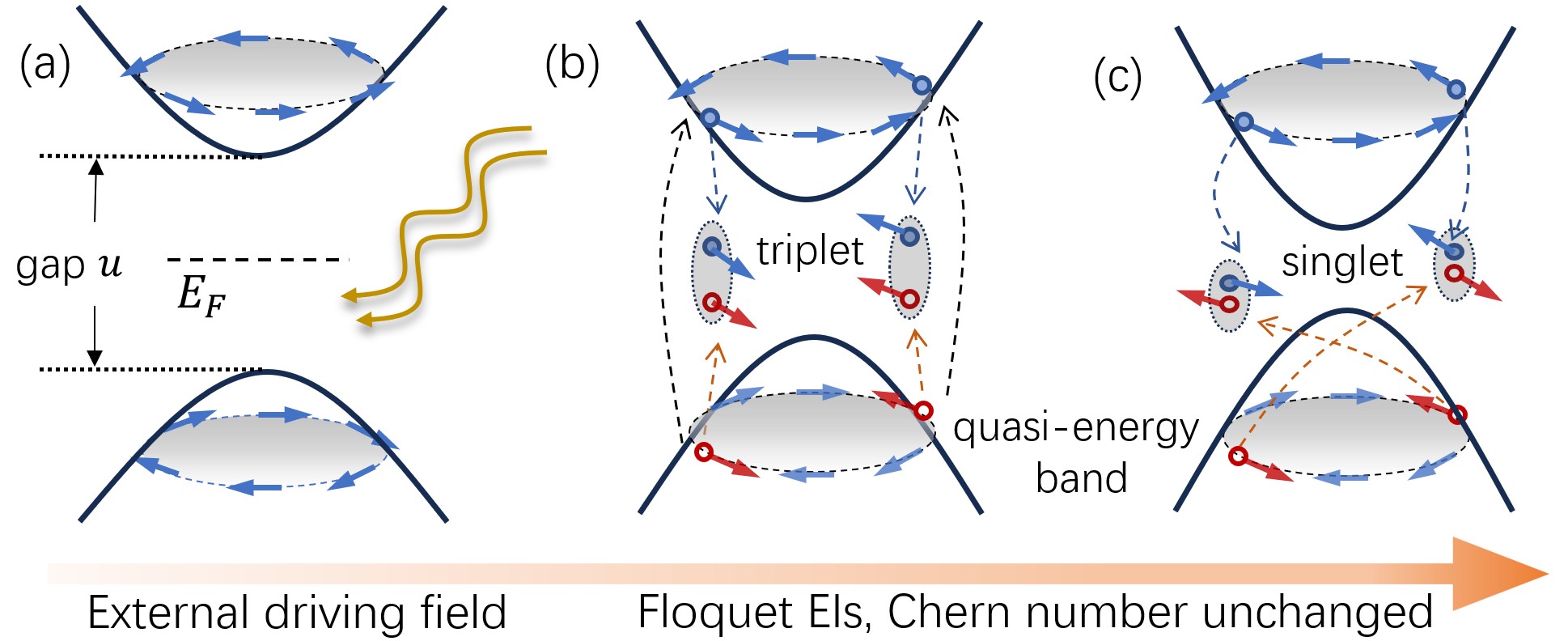
Figure 1: (a) Starting from a TI, the external driving fields can reduce the quasi-energy band gap. (e) For intermediate gap values, a $p+ip$-wave triplet EI can be favored. (f) For small gap values, an s-wave singlet EI is stabilized.

In this Letter, we show that the interplay between correlation and quantum geometry points to more exotic phases of matter beyond the topological descriptions. We reveal novel topological excitonic insulators (EIs) exhibiting the same bulk topology but distinct physical properties owing to their different quantum geometries. EIs are correlated insulators extensively studied in recent years [21, 22, 23, 24, 25, 26, 27, 28, 29, 30]. For band insulators (semiconductors) with a gap smaller than the exciton binding energy, the electron-hole interaction is known to spontaneously drive the EI phases with $s$-wave pairing symmetry [21]. Here, we instead start from a topological insulator (TI) exhibting spin-momentum locking (Fig.1(a)). With gradually reducing the band gap, remarkably we find that a $p+ip$ triplet EI is energetically favored in the intermediate gap regime. Only when the gap is reduced to small values, does the conventional $s$-wave singlet EI becomes stable, as shown by Fig.1(c). Notably, all the three insulating phases, i.e., the original TI, the $p+ip$ and the $s$-wave EI, exhibit the same Chern number. However, they display completely different physical properties including the spin textures and the magnetic-optical Kerr effects. Such differences reveal the important role of quantum geometry in shaping correlated states [31, 32, 33, 34, 35] and their physical natures.

To observe the quantum geometry enriched topological EIs and their phase transitions, the band gap needs to be tuned. This can be achieved by Floquet engineering via application of a periodic driving field. As shown by Fig.1, we show that a high frequency driving field can continuously reduce the quasi-energy band gap. This efficiently enhances the correlation effect, stabilizing the quantum geometry enriched Floquet topological EIs (FTEIs). Our work therefore suggests (1) a systematic way to modulate the correlation effect via Floquet engineering, and (2) reveals new correlated phenomena enriched by quantum geometry.

Floquet-enhanced correlation effect.– We consider the minimal model of an interacting topological insulator. The free part, in the basis of $\Phi_{\mathbf{k}}=[f_{\mathbf{k},\uparrow},f_{\mathbf{k},\downarrow}]^{\mathrm{T}}$, is given by, $H_{0}=\sum_{\mathbf{k}}\Phi^{\dagger}_{\mathbf{k}}(v_{F}\boldsymbol{\sigma}\cdot\mathbf{k}+u\sigma_{z})\Phi_{\mathbf{k}}$, where the Pauli matrix $\boldsymbol{\sigma}=(\sigma_{x},\sigma_{y})$ acts in the spin space. $H_{0}$ describes a Dirac fermion in two-dimensions (2D) with spin-momentum locking and a gap $u$. This can be realized in the surface of 3D TIs [36], either by magnetic doping [37, 38] or surface state coupling [39] in thin films consisting of several quintuple layers. An energy cutoff $v_{F}\Lambda$ is implicit in the low-energy effective description, and we set $v_{F}=1$. On top of $H_{0}$, we further consider the Hubbard-type interaction, $H_{\mathrm{int}}=U\sum_{\mathbf{r}}f^{\dagger}_{\mathbf{r},\uparrow}f_{\mathbf{r},\uparrow}f^{\dagger}_{\mathbf{r},\downarrow}f_{\mathbf{r},\downarrow}$.

For large $u$, the gap dominates over the interaction, resulting in a 2D TI characterized by a half-integer Chern number $C=1/2$ [40, 41, 23]. We then consider a periodic in-plane electric field with frequency $\omega$ described by the vector potential $\mathbf{A}(t)=(A\sin(\omega t),A\sin(\omega t+\phi))$, where $\phi$ is the polarization angle and $A$ is the field strength. $\mathbf{A}(t)$ brings about dynamics absent in $H=H_{0}+H_{\mathrm{int}}$, described by $H^{\prime}(t)=v_{F}\sum_{\mathbf{k}}\Phi^{\dagger}_{\mathbf{k}}\boldsymbol{\sigma}\cdot\mathbf{A}(t)\Phi_{\mathbf{k}}$, leading to the total Hamiltonian $H^{\mathrm{tot}}(t)=H+H^{\prime}(t)$. Using the Floquet theory [42, 43], the dynamics over time spans longer than the period $T=2\pi/\omega$ can be separated from the micromotion within $T$ [44]. The stroboscopic time evolution in steps of $T$ is then described by the Floquet Hamiltonian $H_{F}$. The latter not only generates the quasi-energy but also enables tailoring of novel non-equilibrium steady states, i.e., Floquet engineering [45, 46, 47, 48, 49, 50].

We resort to the extended Floquet space, $\mathcal{F}=\mathcal{H}\otimes\mathcal{T}$, a product of the Hilbert space of the quantum system ($\mathcal{H}$), and the space of square-integrable time-dependent function with period $T$ ($\mathcal{T}$). The orthonormal complete basis expanding $\mathcal{F}$ is constructed by $|\alpha\nu(t)\rangle=|\alpha\rangle e^{i\nu\omega t}$, where $\nu\in\mathbb{Z}$ and $|\alpha\rangle$ is the many-body basis of $\mathcal{H}$. Meanwhile, the time-dependent Schördinger equation is cast into the eigenvalue problem of the quasienergy operator $Q(t)=H^{\mathrm{tot}}(t)-i\partial_{t}$. In the extended basis, $Q(t)$ is cast into the matrix, $Q_{\alpha^{\prime}\nu^{\prime},\alpha\nu}=\langle\alpha^{\prime}\nu^{\prime}(t)|Q(t)|\alpha\nu(t)\rangle$ and reads as,

$$Q_{\alpha^{\prime}\nu^{\prime},\alpha\nu}=\langle\alpha^{\prime}|H^{\mathrm{tot}}_{\nu^{\prime}-\nu}|\alpha\rangle+\delta_{\nu^{\prime}\nu}\delta_{\alpha^{\prime}\alpha}\nu\omega,$$ (1)

where $H^{\mathrm{tot}}_{\nu}=\frac{1}{T}\int^{T}_{0}dte^{-i\nu\omega t}H^{\mathrm{tot}}(t)$. Evaluating the eigenvalues of $Q_{\alpha^{\prime}\nu^{\prime},\alpha\nu}$ is challenging, in particular for our case with many-body interaction, $H_{int}$. We thus formally block diagonalize $Q_{\alpha^{\prime}\nu^{\prime},\alpha\nu}$ in the $\mathcal{T}$ space, generating $Q_{\alpha^{\prime}\alpha,\nu^{\prime}\nu}=U_{\nu^{\prime}l}Q_{\alpha^{\prime}\alpha,l}U^{\star}_{l\nu}$, and $Q_{\alpha^{\prime}\alpha,l}$ is of the form, $Q_{\alpha^{\prime}\alpha,l}=\langle\alpha^{\prime}|H_{F}|\alpha\rangle+\delta_{\alpha^{\prime}\alpha}l\omega$, where $l$ is the Floquet band index. The Floquet Hamiltonian $H_{F}$ here is our main focus, as it determines the quasi-energy and the stroboscopic evolution of quantum states.

A systematic way to compute $H_{F}$ is the high-frequency expansion [44]. For $\omega$ larger than the off-diagonal components ($\nu^{\prime}\neq\nu$) in Eq.(1), the degenerate perturbation calculation can be performed, which generates $H_{F}=H^{\mathrm{tot}}_{0}+[H^{\mathrm{tot}}_{1},H^{\mathrm{tot}}_{-1}]/\omega+O(\omega^{-2})$. Here, since the interaction $H_{\mathrm{int}}$ does not have time-dependence, its Fourier component is involved in the diagonal component $H^{\mathrm{tot}}_{0}$. We note that the presence of $H_{\mathrm{int}}$ will introduce further corrections to $H_{F}$ in the high-frequency expansion. However, the leading corrections do not occur until the third order perturbation ($\propto O(\omega^{-2})$) [51]. Thus, they can be neglected for high frequency fields with $\omega>D>\frac{A^{2}}{\omega}$, where $D=\sqrt{u^{2}+\Lambda^{2}}$ (see supplemental materials).

Explicitly calculating $[H^{\mathrm{tot}}_{1},H^{\mathrm{tot}}_{-1}]$ and focusing on the $l=0$ Floquet band [44], we arrive at the second-quantized effective interacting Hamiltonian as,

$$H_{\mathrm{eff}}=\sum_{\mathbf{k}}\Phi^{\dagger}_{\mathbf{k},0}(\sigma\cdot\mathbf{k}+m\sigma_{z})\Phi_{\mathbf{k},0}+U\sum_{\mathbf{r}}n_{\mathbf{r},0,\uparrow}n_{\mathbf{r},0,\downarrow},$$ (2)

where $\Phi_{\mathbf{k},0}=[f_{\mathbf{k},0,\uparrow},f_{\mathbf{k},0,\downarrow}]^{\mathrm{T}}$, $n_{\mathbf{r},0,\sigma}=f^{\dagger}_{\mathbf{r},0,\sigma}f_{\mathbf{r},0,\sigma}$, and $f^{\dagger}_{\mathbf{r},0,\sigma}$ ($f_{\mathbf{r},0,\sigma}$) denotes the creation (annihilation) operator for electrons on the 0-th Floquet band. The gap $m$ is obtained as, $u+\frac{A^{2}}{\omega}\sin(\phi)$, and we focus on the circular polarization ($\phi=-\pi/2$) in the following. Interestingly, $H_{\mathrm{eff}}$ has a form similar to that of the undriven model but with a renormalized quasi-energy gap $m$. Since the gap is reduced, while the strength of interaction $U$ remains intact, the correlation effect is effectively enhanced. This would favor excitonic instabilites as illustrated by Fig.1.

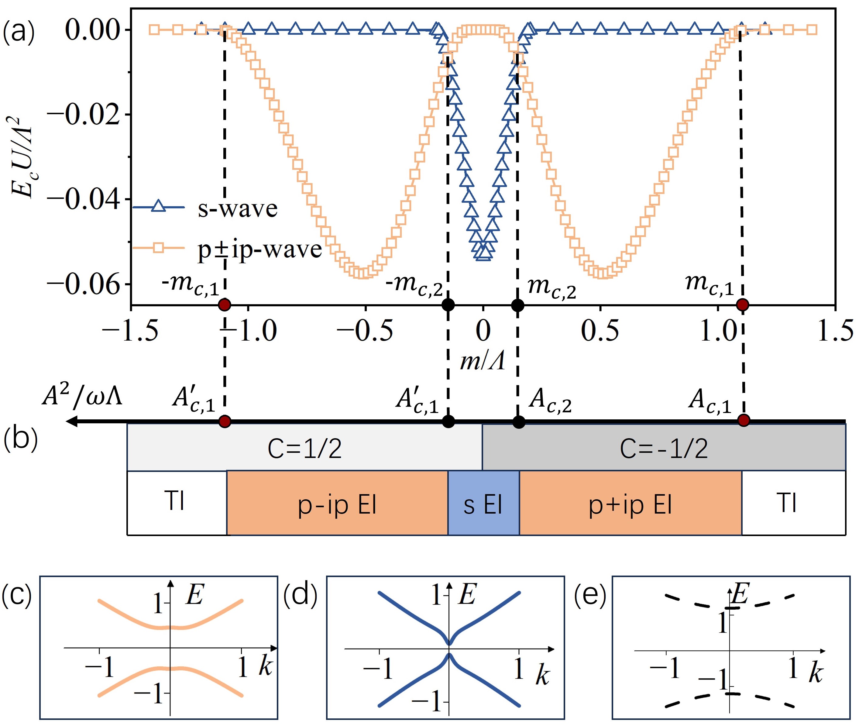
Figure 2: (a) The condensation energy of different phases with varying the renormalized gap $m$. Two transitions occur at $|m_{c,1}|=1.12$ and $|m_{c,2}|=0.15$. (b) The phase diagram versus the field strength $A$. (c)(d)(e) respectively show the characteristic energy spectrum for the $p\pm ip$ EI, $s$-wave EI, and TI.

Quantum geometry enriched FTEIs.– We now study the Floquet excitonic phases based on Eq.(2). Excitons are bound states formed by the conduction electrons and the valence band holes. Thus, we convert to the band basis via the transformation, $[c_{\mathbf{k}},v_{\mathbf{k}}]^{\mathrm{T}}=R\Phi_{\mathbf{k},0}$, where $c_{\mathbf{k}}$ and $v_{\mathbf{k}}$ denote the annihilation operator for Floquet modes on conduction and valance band. The matrix entries are $R_{11}=\cos\theta_{k}e^{i\phi_{\mathbf{k}}}$, $R_{12}=\sin\theta_{k}$, $R_{21}=\sin\theta_{k}e^{i\phi_{\mathbf{k}}}$, $R_{22}=-\cos\theta_{k}$, and $\cos\theta_{k}=\frac{k}{\sqrt{k^{2}+(\epsilon_{k}-m)^{2}}}$, $\sin\theta_{k}=\frac{\epsilon_{k}-m}{\sqrt{k^{2}+(\epsilon_{k}-m)^{2}}}$, where $\mathbf{k}=ke^{i\phi_{\mathbf{k}}}$ and $\epsilon_{k}=\sqrt{k^{2}+m^{2}}$. The dispersion then reads as, $E_{\pm,k}=\pm\epsilon_{k}$.

The second term in Eq.(2) needs to be accordingly projected to the band basis. With focusing on the interband interactions in the forward scattering channel that favor excitonic instabilities [23], we arrive at the relevant interaction as [51],

$$\begin{split}H^{\mathrm{eff}}_{\mathrm{int}}=U&\sum_{\mathbf{k},\mathbf{k}^{\prime}}[\cos^{2}\theta_{k}\cos^{2}\theta_{k^{\prime}}e^{i(\phi_{\mathbf{k}}-\phi_{\mathbf{k}^{\prime}})}\\ &+\sin^{2}\theta_{k}\sin^{2}\theta_{k^{\prime}}e^{i(\phi_{\mathbf{k}^{\prime}}-\phi_{\mathbf{k}})}\\ &+2\cos\theta_{k}\cos\theta_{k^{\prime}}\sin\theta_{k}\sin\theta_{k^{\prime}}]c^{\dagger}_{\mathbf{k}}v^{\dagger}_{\mathbf{k}^{\prime}}v_{\mathbf{k}}c_{\mathbf{k}^{\prime}}.\end{split}$$ (3)

For the $\phi_{\mathbf{k}}$-independent term in Eq.(3), we introduce the excitonic order parameter, $\Delta_{s}=U\sum_{\mathbf{k}}\cos\theta_{k}\sin\theta_{k}\langle c^{\dagger}_{\mathbf{k}}v_{\mathbf{k}}\rangle$, with isotropic s-wave pairing. For the $\phi_{\mathbf{k}}$-dependent terms, two $p$-wave pairing orders can be respectively introduced, i.e., $\Delta_{p,1}=U\sum_{\mathbf{k}}\cos^{2}\theta_{k}e^{i\phi_{\mathbf{k}}}\langle c^{\dagger}_{\mathbf{k}}v_{\mathbf{k}}\rangle$, and $\Delta_{p,2}=U\sum_{\mathbf{k}}\sin^{2}\theta_{k}e^{-i\phi_{\mathbf{k}}}\langle c^{\dagger}_{\mathbf{k}}v_{\mathbf{k}}\rangle$. These describe $p\pm ip$ excitonic insulators, as they generate off-diagonal terms in the mean-field Hamiltonian that are proportional to $(k_{x}\pm ik_{y})/k$. Inserting the order parameters into Eq.(3) and minimizing the mean-field ground state energy, we self-consistently determine the condensation energy and the phase diagram with varying $A$.

The condensation energy $E_{c}$, defined as the energy difference between the mean-field phases and the free state, is shown in Fig.2(a). For small $A$ (large $m$), the band gap $m$ dominates over the interaction $U$, and the Floquet TI with $C=-1/2$ is stable. For larger $A$ with $A^{2}/\omega\lesssim u$, such that the gap is renormalized to small values ($m\gtrsim 0$), $U$ plays the dominant role. In this case, the excitonic orders is formed with the isotropic $s$-wave pairing, i.e., $\Delta_{s}\neq 0$. Interestingly, in the intermediate region, we find that a $p+ip$-wave Floquet EI becomes stable, with $\Delta_{p,1}\neq 0$, $\Delta_{s}=0$. Notably, the Chern number for both the $s$-wave and $p+ip$-wave Floquet EI maintain the same as that of the initial Floquet TI, i.e., $C=-1/2$. With further increasing $A$, $m$ changes its sign, three mass-inverted states are found, including the $s$-wave, the $p-ip$ wave EI, and the TI, as shown by Fig.2. These are the time-reversal symmetry (TRS)-inverted counterparts for those found in $m>0$, and they exhibit the opposite Chern number, $C=1/2$. The results in Fig.2(b) clearly shows two successive transitions with tuning $m$ (or $A$), i.e., from the Floquet TI to the $p\pm ip$ EI (at $\pm m_{c,1}$) and then to the $s$-wave EI (at $\pm m_{c,2}$) .

The single-particle Hamiltonian of the TI can be written compactly as, $H_{\mathrm{TI}}=\boldsymbol{\sigma}\cdot\mathbf{d}_{\mathrm{TI}}$, where $\mathbf{d}_{\mathrm{TI}}=(k_{x},k_{y},m)$. The mean-field Hamiltonians of the $s$- and $p+ip$-wave EI are then accordingly obtained as, $H_{\mathrm{EI},s/p}=\boldsymbol{\sigma}\cdot(\mathbf{d}_{\mathrm{TI}}+\delta\mathbf{d}_{s/p})$, where $\delta\mathbf{d}_{s}=(\frac{m\Delta_{s}k_{x}}{\epsilon^{2}_{k}},\frac{m\Delta_{s}k_{y}}{\epsilon^{2}_{k}},-\frac{\Delta_{s}k^{2}}{\epsilon^{2}_{k}})$, and $\delta\mathbf{d}_{p}=(\frac{\Delta_{p,1}(k^{2}_{y}+m^{2}+m\epsilon_{k})}{2\epsilon^{2}_{k}},-\frac{\Delta_{p,1}k_{x}k_{y}}{2\epsilon^{2}_{k}},-\frac{\Delta_{p,1}k_{x}(m+\epsilon_{k})}{2\epsilon^{2}_{k}}$). Interestingly, although TRS is further broken by both $\delta\mathbf{d}_{s}$ and $\delta\mathbf{d}_{p}$, the way how it is broken is different. For the s-wave case, TRS is violated by the z-component, $\delta d_{s,z}$. However, for the $p+ip$ wave case, it is violated by the in-plane components, $\delta d_{s,x}$ and $\delta d_{s,y}$. Such a different symmetry property leads to distinct energy spectra shown in Fig.2(c)-(e).

Given that both the $s$- and $p+ip$-wave FTEIs exhibit the same Chern number, their physical differences are not characterized by topology. We therefore examine their distinctions regarding the quantum geometry. The geometric information is contained in the Fubini-Study tensor [52, 9], i.e., $\mathbb{B}_{ij}(\mathbf{k})=\langle\partial_{i}u_{\mathbf{k}}|\partial_{j}u_{\mathbf{k}}\rangle-\langle\partial_{i}u_{\mathbf{k}}|u_{\mathbf{k}}\rangle\langle u_{\mathbf{k}}|\partial_{j}u_{\mathbf{k}}\rangle$, where $|u_{\mathbf{k}}\rangle$ is the wavefunction defined in the momentum space and $\partial_{i}=\frac{\partial}{\partial k_{i}}$ with $i=x,y$ . Our main focus is the real part of $\mathbb{B}_{ij}$, i.e., the quantum metric measuring the distance between adjacent quantum states.

To better quantify the quantum geometry for the three phases, we calculate their quantum volumes, defined as [53, 54] $g=\int\mathbf{k}\sqrt{\mathrm{det~{}Re}[\mathbb{B}_{ij}(\mathbf{k})]}$, as well as the radial distribution of the quantum volume, $g(k)=\int^{2\pi}_{0}d\phi_{\mathbf{k}}k\sqrt{\mathrm{det~{}Re}[B_{ij}(\mathbf{k})]}$. As shown by Fig.3(a), $g(k)$ generally increases with $k$ for the TI parent state. For the $p+ip$ Floquet EI, $g(k)$ is enhanced and exhibits a wide peak feature. For the $s$-wave EI, $g(k)$ however undergoes significant changes, displaying a more complicated non-monotonous behavior. A rapid increase occurs for small $k$ before decreasing down to $g(k)=0$, which again raises slightly for larger $k$.

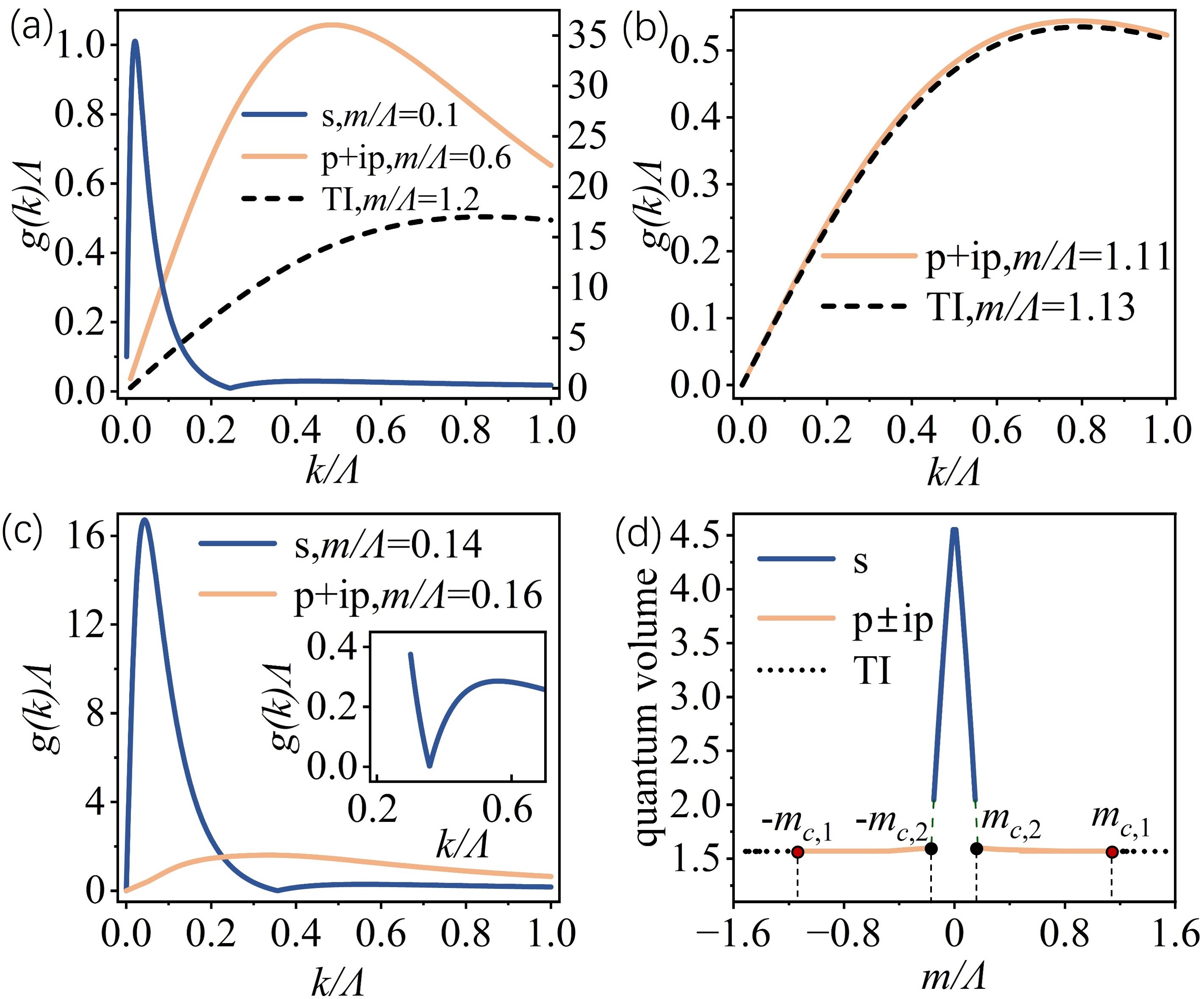
Figure 3: Comparison of the quantum geometry of three topological insulators. (a) The $k$-distribution of the quantum volume $g(k)$. The left (right) axis corresponds to the $p+ip$ EI and the TI ($s$-wave EI). (b) The change of $g(k)$ crossing the $p+ip$ EI-TI transition (at $m_{c,1}=1.12$ in Fig.2). (c) The change of $g(k)$ crossing the $s$-$p$ wave FTEI transition at $m_{c,2}=0.15$. (d) The evolution of quantum volume with varying $m$.

We further examine the change of $g(k)$ crossing the two transition points, $m_{c,1}$ and $m_{c,2}$. As shown by Fig.3(b), $g(k)$ evolves smoothly crossing the $p+ip$ EI-TI transition at $m_{c,1}$. However, an abrupt change occurs at the $p+ip$ EI-$s$ wave EI transition at $m_{c,2}$ (Fig.3(c)). Moreover, the evolution of the quantum volume $g$ with varying $m$ also reveals a sudden jump at $m_{c,2}$ (Fig.3(d)). This clearly indicates that the wavefunction of the $p+ip$ EI and its quantum geometry are in resemblance with those of the TI state, while in sharp difference with the $s$-wave EI. With lowering $|m|$ (enhancing the correlation effect), the wavefunction would intend to maintain the minimal change during phase transitions. This accounts for why the TI firstly undergoes the transition to the $p+ip$ EI, and then to the $s$-wave EI, in consistence with the energetics shown in Fig.2(a)(b).

Spin textures and magneto-optical Kerr responses.– So far we have revealed three Floquet insulators with the same topology but different quantum geometries. The distinct geometries should lead to different physical properties. One direct reflection is the ground state spin texture, defined as $s_{i}(\mathbf{k})=\langle\sigma_{i}\rangle/2$ ($i=x,y,z$), where $\langle...\rangle$ denotes the average over the mean-field ground state of the three phases, $|\phi_{\mathbf{k}}\rangle$. We plot the total spin polarization along $z$, i.e., $M_{z}=\int d\mathbf{k}s_{z}(\mathbf{k})$ in Fig.4(a). As shown, with decreasing $|m|$, the evolution of $S_{z}$ is smooth during the transition from the TI to the $p\pm ip$ EI. This is due to the fact that $\delta d_{p,z}$ does not violate TRS. In contrast, $M_{z}$ exhibits a sudden jump at the transition from the $p\pm ip$ to the $s$-wave EI, reflecting that TRS is further broken by $\delta d_{s,z}$.

Interestingly, the two EIs also display completely different in-plane spin textures, $\mathbf{s}_{\mathrm{in}}=(s_{x}(\mathbf{k}),s_{y}(\mathbf{k}))$, as shown in Fig.4(b)(c). An anisotropic spin texture is found for the $p+ip$ case, in contrast to the isotropic texture for the $s$-wave EI. Thus, a finite in-plane magnetization, $\mathbf{M}_{\mathrm{in}}=(M_{x},M_{y})=\int d\mathbf{k}\mathbf{s}_{\mathrm{in}}(\mathbf{k})$, emerges for the $p+ip$ EI, absent in the $s$-wave case. Such characteristic magnetizations could be probed via the measurement of spin susceptibility [55].

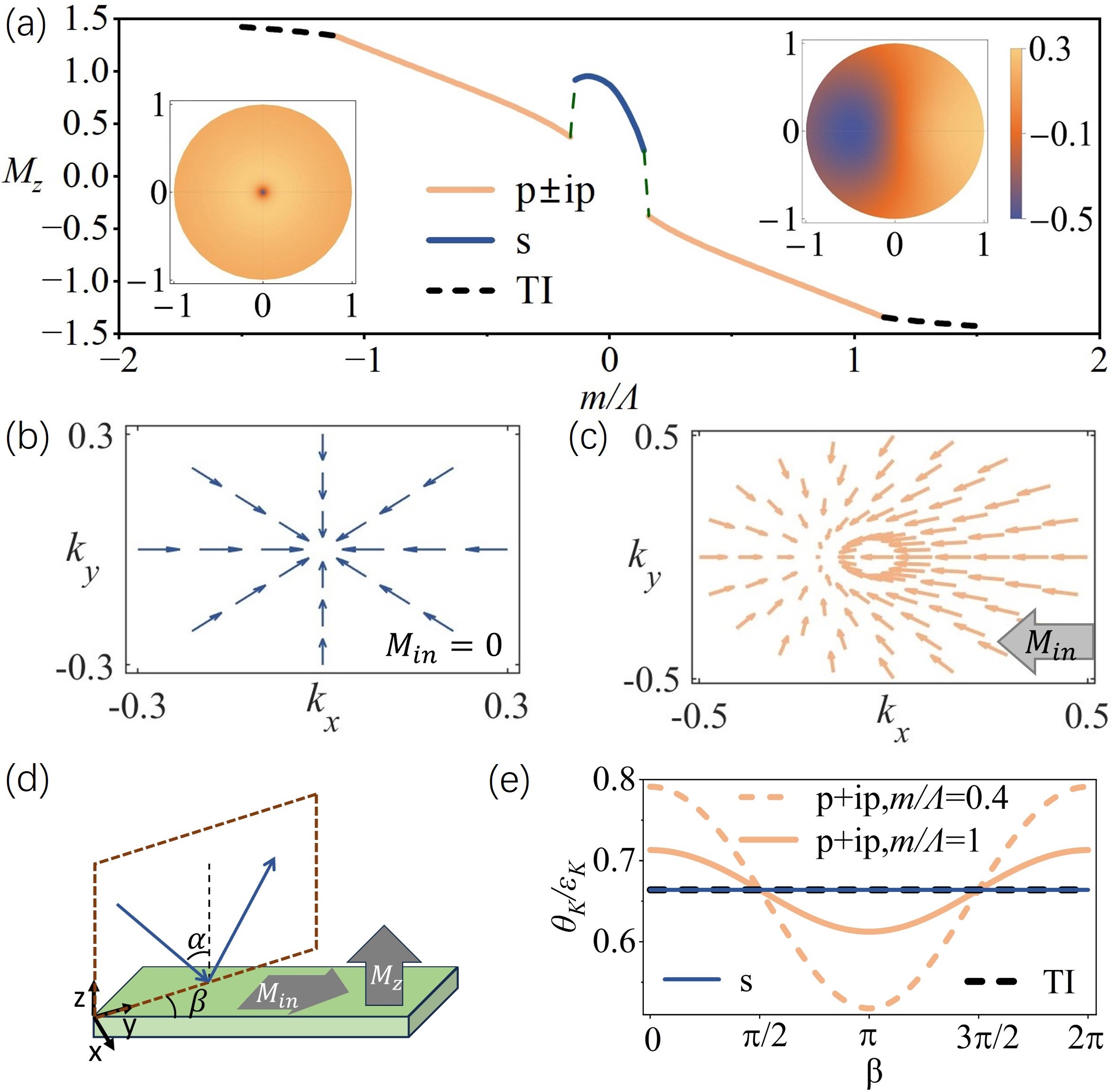
Figure 4: (a) The magnetization $M_{z}$ with tuning $m$. The left (right) inset show the distribution $s_{z}(\mathbf{k})$ over momentum space for the s-wave ($p+ip$ wave) EI. (b) and (c) are the in-plane spin textures for the s-wave and $p+ip$ wave EI. (d) Schemcatic plot of the setup that demonstrates the MOKE. (e) The ratio between the Kerr angle and ellipticity versus the angle of the incident plane.

The different quantum geometries and magnetizations can also be detected via the magneto-optical Kerr effect (MOKE). We consider applying a linear polarized light incident onto the 2D surface states, as indicated Fig.4(d)). The reflected light will then display both the Kerr rotation $\theta_{K}$ and the ellipticity $\epsilon_{K}$, which are determined by the dielectric tensor $\varepsilon$ of the material. For the $s$-wave EI, the magnetization is out-of-plane ($z$-direction) thus it displays the polar MOKE [56]. The dielectric tensor $\varepsilon$ for this case has U(1) rotation symmetry about $z$ axis. After a coordinate rotation, the general form of $\varepsilon$ can be obtained for magnetization along arbitrary direction [51, 57, 58, 56]. Assuming that the electric field vector of the light being perpendicular to the incident plane, $\theta_{K}$ and $\varepsilon_{K}$ are derived to satisfy [51],

$$\begin{split}&\theta_{K}+i\varepsilon_{K}\\ &=\frac{in_{1}n_{2}Q\cos\alpha_{1}(\overline{M}_{y}\sin\alpha_{2}+\overline{M}_{z}\cos\alpha_{2})}{\cos\alpha_{2}(n_{2}\cos\alpha_{1}+n_{1}\cos\alpha_{2})(n_{1}\cos\alpha_{1}-n_{2}\cos\alpha_{2})},\end{split}$$ (4)

where $\overline{M}_{i}=M_{i}/|\mathbf{M}|$ is the normalized magnetization, $n_{1}$ and $n_{2}$ are respectively the complex refractive index of the vacuum and the material, $\alpha_{1}$ and $\alpha_{2}$ are the incident and reflective angle, and $Q$ is the magneto-optical Voigt constant, which can be experimentally measured. Equating the real and imaginary part in Eq.(4) and inserting the magnetization of the three insulating states, we then obtain the ratio $\theta_{K}/\varepsilon_{K}$.

We plot $\theta_{K}/\varepsilon_{K}$ in Fig.4(e) with rotating the incident plane, i.e., the angle $\beta$ in Fig.4(d). As shown, for both the TI and the s-wave topological EI, $\theta_{K}/\varepsilon_{K}$ remains a constant with rotating $\beta$. This is because the TI and the s-wave EI only have out-of-plane magnetization $\overline{M}_{z}$, thus the Kerr response remains rotational invariant with respect to $\beta$. In contrast, the $p+ip$ EI shows a periodic response behavior, whose amplitude decreases with increasing $|m|$ . Thus, with tuning the driving field $A$, $\theta_{K}/\varepsilon_{K}$ would undergo a nonmonotonous evolution, from a constant behavior to a periodic response, and then back to the constant. The spin texture and the MOKE reveal novel properties of FTEIs that are not captured by their topology, but enriched by quantum geometry.

Conclusion and discussion.– It is known for decades that $s$-wave EIs can be spontaneously formed for insulators with a gap smaller than the exciton binding energy [21]. Here, we however show that, if the initial state is a TI, novel $p\pm ip$ topological EIs can emerge as an intermediate state (Fig.1). Although this is beyond conventional understandings, it is a natural result from the perspective of quantum geometry. This is because the wavefunction changes in a much more moderate way (in terms of the quantum geometry, Fig.3(b)) during the transition from the TI to the $p\pm ip$ EI. Moreover, the different quantum geometry between the $p\pm ip$ and $s$-wave EI results in essentially different physical properties, such as the spin textures and MOKE. In addition, we also show that the insulator gap can be effectively reduced in an non-equilibrium fashion via Floquet engineering. This can significantly enhance the correlation effect, pointing to a new promising direction, i.e., exploration of quantum geometry enriched Floquet correlated phases.

Supplemental material for:Quantum Geometry Enriched Floquet Topological Excitonic Insulators

We provide supplemental information regarding technical details on the derivations of key conclusions presented in the manuscript. The specific contents include: (1) Floquet engineering of the band gap, (2) Quantum volume, (3) Magneto-optical Kerr effect.

I Floquet engineering of the band gap

We start from the Hamiltonian of interacting massive Dirac fermions, i.e.,

$$\begin{split}H=&\sum_{\mathbf{k}}\Phi^{\dagger}_{\mathbf{k}}[v_{F}(k_{x}\sigma_{x}+k_{y}\sigma_{y})+u\sigma_{z}]\Phi_{\mathbf{k}}+H_{\mathrm{int}}\\ =&\sum_{\mathbf{k}}\left(\begin{matrix}f^{\dagger}_{\mathbf{k},\uparrow}&f^{\dagger}_{\mathbf{k},\downarrow}\end{matrix}\right)\left(\begin{matrix}u&v_{F}(k_{x}-ik_{y})\\ v_{F}(k_{x}+ik_{y})&-u\end{matrix}\right)\left(\begin{matrix}f_{\mathbf{k},\uparrow}\\ f_{\mathbf{k},\downarrow}\end{matrix}\right)+U\sum_{\mathbf{k},\mathbf{k^{\prime}},\mathbf{q}}f^{\dagger}_{\mathbf{k+q},\uparrow}f^{\dagger}_{\mathbf{k^{\prime}-q},\downarrow}f_{\mathbf{k^{\prime}},\downarrow}f_{\mathbf{k},\uparrow},\end{split}$$ (1)

where $\Phi_{\mathbf{k}}=[f_{\mathbf{k},\uparrow},f_{\mathbf{k},\downarrow}]^{T}$ and hereafter we set Fermi velocity $v_{F}$ to 1. An energy cutoff $\Lambda$ is implicit in the kinetic energy term of Eq.(1). We then apply the periodic driving field, which drives the kinetic energy, i.e., into the first term in Eq.(1),

$$H^{\mathrm{kin}}_{\mathbf{k}}(t)=\left(\begin{matrix}u&(k_{x}+A\sin\omega t)-i(k_{y}+A\sin(\omega t+\phi))\\ (k_{x}+A\sin\omega t)+i(k_{y}+A\sin(\omega t+\phi))&-u\end{matrix}\right).$$ (2)

We then proceed by performing a Fourier expansion of the total time-dependent Hamiltonian $H^{\textrm{{tot}}}(t)=\sum_{\mathbf{k}}\Phi^{\dagger}_{\mathbf{k}}H^{\textrm{{kin}}}_{\mathbf{k}}(t)\Phi_{\mathbf{k}}+H_{\mathrm{int}}$, which is cast into:

$$H^{\mathrm{tot}}=H^{\mathrm{tot}}_{0}+H^{\mathrm{tot}}_{1}e^{i\omega t}+H^{\mathrm{tot}}_{-1}e^{-i\omega t}.$$ (3)

Since $H_{\mathrm{int}}=U\sum_{\mathbf{k},\mathbf{k^{\prime}},\mathbf{q}}f^{\dagger}_{\mathbf{k+q},\uparrow}f^{\dagger}_{\mathbf{k^{\prime}-q},\downarrow}f_{\mathbf{k^{\prime}},\downarrow}f_{\mathbf{k},\uparrow}$ is time-independent, it is only involved in the component, $H^{\mathrm{tot}}_{0}$. Whereas, the kinetic energy term $H^{\mathrm{kin}}(t)=\sum_{\mathbf{k}}\Phi^{\dagger}_{\mathbf{k}}H^{\textrm{{kin}}}_{\mathbf{k}}(t)\Phi_{\mathbf{k}}$ generates all three nonzero components in Eq.(3). Thus, we obtain,

$$H^{\mathrm{tot}}_{0}=H^{\mathrm{kin}}_{0}+H_{\mathrm{int}}=\sum_{\mathbf{k}}\Phi^{\dagger}_{\mathbf{k}}\left(\begin{matrix}u&k_{x}-ik_{y}\\ k_{x}+ik_{y}&-u\end{matrix}\right)\Phi_{\mathbf{k}}+H_{\mathrm{int}}.$$ (4)

and the Fourier components of Hamiltonian of $H^{\mathrm{int}}_{\mathbf{k}}$ reads as,

$$H^{\mathrm{tot}}_{1}=H^{\mathrm{kin}}_{1}=\sum_{\mathbf{k}}\Phi^{\dagger}_{\mathbf{k}}\left(\begin{matrix}0&A(\frac{1}{2i}-\frac{e^{i\phi}}{2})\\ A(\frac{1}{2i}+\frac{e^{i\phi}}{2})&0\end{matrix}\right)\Phi_{\mathbf{k}},$$ (5)

$$H^{\mathrm{tot}}_{1}=H^{\mathrm{kin}}_{1}=\sum_{\mathbf{k}}\Phi^{\dagger}_{\mathbf{k}}\left(\begin{matrix}0&A(-\frac{1}{2i}+\frac{e^{-i\phi}}{2})\\ A(-\frac{1}{2i}-\frac{-e^{-i\phi}}{2})&0\end{matrix}\right)\Phi_{\mathbf{k}}.$$ (6)

In high frequency expansion, the effective Floquet Hamiltonian can be calculated as,

$$H_{\mathrm{eff}}=H^{\mathrm{tot}}_{0}+\sum_{m\neq 0}\frac{H^{\mathrm{tot}}_{m}H^{\mathrm{tot}}_{-m}}{m\omega}+\sum_{m\neq 0}\frac{[H^{\mathrm{tot}}_{-m},[H^{\mathrm{tot}}_{0},H^{\mathrm{tot}}_{m}]]}{2(m\omega)^{2}}+O(\omega^{-2})$$ (7)

The above expansion stands in following perturbative sense [44]. The energy scale of $H_{0}$ is $\sim D=\sqrt{u^{2}+\Lambda^{2}}$ (and $H_{int}\sim\Lambda$ is taken in the manuscript). The Floquet field modulate system mainly by the first order term in Eq.(7), i.e., $A^{2}/\omega$. Meanwhile, the second term in Eq.(7), i.e., $\frac{A^{2}D}{\omega^{2}}$ can be disregarded in the condition, $D>\frac{A^{2}}{\omega}>\frac{A^{2}D}{\omega^{2}}$, i.e., $\omega\gg D>\frac{A^{2}}{\omega}$. Clearly, this automatically ensures that the different Floquet bands do not overlap over each other. Notably, it is also known from Eq.(7) that the four-fermion interaction term does not get renormalized until the second order correction, which is negligible under the above high-frequency condition.

To the first order correction, we arrive at,

$$H_{\mathrm{eff}}=\sum_{\mathbf{k}}\Phi^{\dagger}_{\mathbf{k},0}\left(\begin{matrix}u+\frac{A^{2}\sin\phi}{\omega}&k_{x}-ik_{y}\\ k_{x}+ik_{y}&-u-\frac{A^{2}\sin\phi}{\omega}\end{matrix}\right)\Phi_{\mathbf{k},0}+H_{\mathrm{int}}.$$ (8)

The first term of Eq.(8) gives rise to the following energy spectrum,

$$\epsilon_{\mathbf{k}}=\pm\sqrt{k^{2}+(u+\frac{A^{2}}{\omega}\sin(\phi))^{2}}.$$ (9)

For the circularly polarization, $\phi=-\frac{\pi}{2}$ , the Floquet Hamiltonian is reduced to that in the main text, with the effective energy gap, $m=u-\frac{A^{2}}{\omega}$, which is modulated by external driving fields.

II Reduced Hamiltonian of Floquet topological excitonic insulators

The kinetic energy term in Eq.(2) of the main text is diagonalized via the unitary transformation,

$$\left(\begin{matrix}f_{\mathbf{k},0,\uparrow}\\ f_{\mathbf{k},0,\downarrow}\end{matrix}\right)=\left(\begin{matrix}\cos\theta_{k}e^{-i\phi_{\mathbf{k}}}&\sin\theta_{k}e^{-i\phi_{\mathbf{k}}}\\ \sin\theta_{k}&-\cos\theta_{k}\end{matrix}\right)\left(\begin{matrix}c_{\mathbf{k}}\\ v_{\mathbf{k}}\end{matrix}\right).$$ (10)

where $c_{\mathbf{k}}$ and $v_{\mathbf{k}}$ denote the annihilation operator for the Floquet modes on the conduction and valance band, and $\phi_{\mathbf{k}}$ is the angle of $\mathbf{k}$, and $\sin\theta$ and $\cos\theta$ are merely functions determined by $k$ and $m$, as shown in the main text.

We insert the unitary transformation into the interaction term $H_{\mathrm{int}}=U\sum_{\mathbf{k},\mathbf{k^{\prime}},\mathbf{q}}f^{\dagger}_{\mathbf{k+q},0,\uparrow}f^{\dagger}_{\mathbf{k^{\prime}-q},0,\downarrow}f_{\mathbf{k^{\prime}},0,\downarrow}f_{\mathbf{k},0,\uparrow}$ in Eq.(2) of the main text, sixteen different terms are derived describing the scattering between electrons on the conduction and valence bands. Focusing on the terms with energy/momentum conservation and the interband interactions in the forward scattering channel (that favors excitonic instabilities), we can reduce the interaction term to the form tractable by mean-field treatment. For the scattering channel, $\mathbf{k+q=k}$, i.e., $\mathbf{q=0}$, we obtain,

$$\begin{split}H^{(1)}_{\mathrm{int}}=U\sum_{\mathbf{k},\mathbf{k^{\prime}}}[(&\cos^{2}\theta_{k}\cos^{2}\theta_{k^{\prime}}+\sin^{2}\theta_{k}\sin^{2}\theta_{k^{\prime}})c^{\dagger}_{\mathbf{k}}v^{\dagger}_{\mathbf{k^{\prime}}}v_{\mathbf{k^{\prime}}}c_{\mathbf{k}}+2\cos\theta_{k}\cos\theta_{k^{\prime}}\sin\theta_{k}\sin\theta_{k^{\prime}}c^{\dagger}_{\mathbf{k}}v^{\dagger}_{\mathbf{k^{\prime}}}v_{\mathbf{k}}c_{\mathbf{k^{\prime}}}].\end{split}$$ (11)

For the other scattering channel $\mathbf{k+q=k^{\prime}}$, we arrive at

$$\begin{split}&H^{(2)}_{\mathrm{int}}=U\sum_{\mathbf{k},\mathbf{k^{\prime}}}[2\cos(\phi_{\mathbf{k}}-\phi_{\mathbf{k^{\prime}}})\cos\theta_{k}\cos\theta_{k^{\prime}}\sin\theta_{k}\sin\theta_{k^{\prime}}c^{\dagger}_{\mathbf{k}}v^{\dagger}_{\mathbf{k^{\prime}}}v_{\mathbf{k^{\prime}}}c_{\mathbf{k}}]\\ &+U\sum_{\mathbf{k},\mathbf{k^{\prime}}}[\cos^{2}\theta_{k}\cos^{2}\theta_{k^{\prime}}e^{i(\phi_{\mathbf{k}}-\phi_{\mathbf{k^{\prime}}})}+\sin^{2}\theta_{k}\sin^{2}\theta_{k^{\prime}}e^{i(\phi_{\mathbf{k^{\prime}}}-\phi_{\mathbf{k}})}]c^{\dagger}_{\mathbf{k}}v^{\dagger}_{\mathbf{k^{\prime}}}v_{\mathbf{k}}c_{\mathbf{k^{\prime}}}.\\ \end{split}$$ (12)

We note that in the mean-field level, the first term in Eq.(11) and Eq.(12) only generates shift of the chemical potential, which is negligible for insulating phases where the Fermi energy lies in the band gap. Thus, combining $H^{(1)}_{\mathrm{int}}$ and $H^{(2)}_{\mathrm{int}}$, we obtain the reduced interaction relevant to the Floquet excitonic insulator phases, i.e., Eq.(3) of the main text.

III The quantum volume

The matrix element of quantum geometry tensor is given by

$$\mathbb{B}_{ij}(\mathbf{k})=\langle\partial_{i}u_{\mathbf{k}}|\partial_{j}u_{\mathbf{k}}\rangle-\langle\partial_{i}u_{\mathbf{k}}|u_{\mathbf{k}}\rangle\langle u_{\mathbf{k}}|\partial_{j}u_{\mathbf{k}}\rangle,$$ (13)

where $\partial_{i}=\frac{\partial}{\partial_{k_{i}}}$ with $i=x,y$, and $|u_{\mathbf{k}}\rangle$ represents for the $\mathbf{k}$-dependent wavefunction.The quantum volume $g$ is defined as

$$g=\int d\mathbf{k}\sqrt{\mathrm{det}~{}\mathrm{Re}[\mathbb{B}_{ij}(\mathbf{k})]},$$ (14)

where $\mathrm{det}$ denotes determinant of the matrix with $i$, $j$ indices. The quantum volume and its radial distribution for three different phases are shown in Fig.3 of the main text. Here, we show more details regarding its distribution in momentum space. We plot in Fig.1 the function $\sqrt{\mathrm{det}~{}\mathrm{Re}[\mathbb{B}_{ij}(\mathbf{k})]}$. As shown, a singularity at $\mathbf{k}=0$ occurs for the $s$-wave EI case, in sharp contrast to the smooth landscape for the $p+ip$ EI and the TI cases. This reflects the fact that formation of the $s$-wave EI from a spin-momentum locked TI requires a sharp change in terms of the wavefunction and the quantum geometry. Thus, the $p+ip$ wave EI naturally occurs as an intermediate state for moderate interactions.

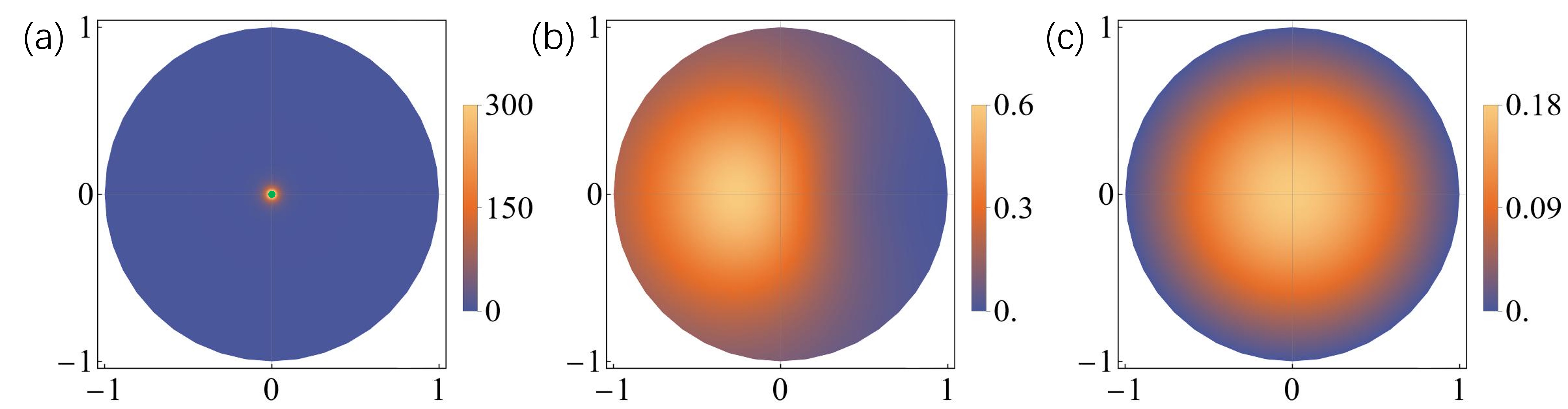
Figure 1: The distribution of quantum volume in $\mathbf{k}$-space of (a) $s$-EI at $m/\Lambda=0.1$, (b) $p+ip$-EI at $m/\Lambda=0.6$ and (c) TI at $m/\Lambda=1.2$.Green dot in (a) means a diverged point.

IV Magneto-optical Kerr effct

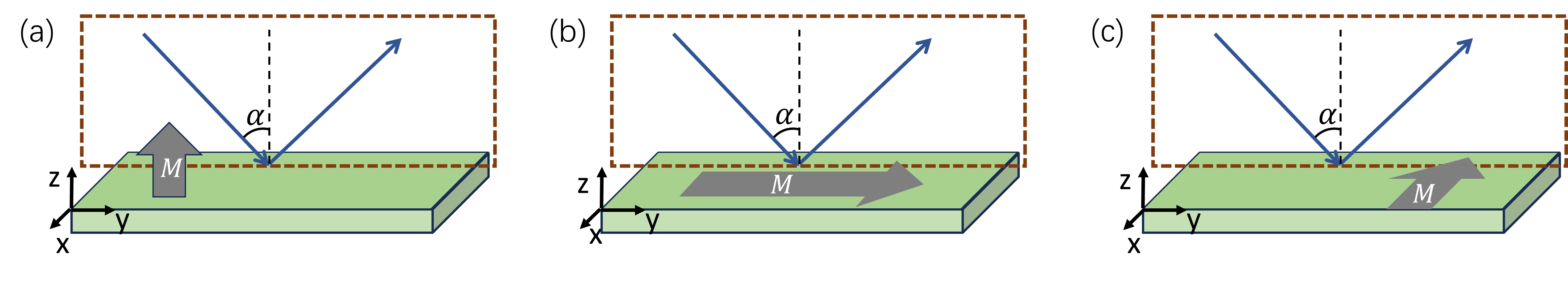
Figure 2: Schematic plot of three different types of MOKEs. (a) Polar MOKE where magnetization is along z-direction. (b) Longitudinal MOKE with the magnetization along y-direction (in parallel with the plane of incidence). (c) Transversal MOKE with the magnetization along y-direction (perpendicular to the plane of incidence).

Magneto-Optical Kerr Effect (MOKE) is usually classified into the polar MOKE (P-MOKE), longitudinal MOKE (L-MOKE), and the transversal MOKE (T-MOKE), as illustrated in Fig. 2. For the P-MOKE, the magnetization is perpendicular to the interface and parallel to the plane of incidence. For the L-MOKE, the magnetization is parallel to the interface as well as plane of incidence. For T-MOKE, the magnetization remains parallel to the interface, but perpendicular to the plane of incidence [57]. Since our revealed Floquet topological excitonic insulators exhibit magnetizations along different directions, one expects they display distinct MOKEs in terms of $\theta_{K}$ and $\epsilon_{K}$.

Note that only the out-of-plane magnetization is present in the ground state of $s$-wave EIs and non-interacting states, which are exactly characterized by the polar geometry depicted in Fig. 2(a). Thus, it is evident that the Kerr signals $\theta_{K}$ and $\epsilon_{K}$ remain unchanged as the plane of incidence (indicated by the dashed box) rotates around the $z$-axis. As shown by the main text, the Kerr rotation and ellipticity satisfy,

$$\begin{split}\theta_{K}+i\epsilon_{K}&=\frac{in_{1}n_{2}Q\cos\alpha_{1}\left(\overline{M}_{y}\sin\alpha_{2}+\overline{M}_{z}\cos\alpha_{2}\right)}{\cos\alpha_{2}\left(n_{2}\cos\alpha_{1}+n_{1}\cos\alpha_{2}\right)\left(n_{1}\cos\alpha_{1}-n_{2}\cos\alpha_{2}\right)},\\ &=\frac{in_{1}n_{2}Q\cos\alpha_{1}\overline{M}_{z}}{\left(n_{2}\cos\alpha_{1}+n_{1}\cos\alpha_{2}\right)\left(n_{1}\cos\alpha_{1}-n_{2}\cos\alpha_{2}\right)}.\end{split}$$ (15)

To quantify the MOKEs, we assume that linearly porlarized incident light is incident from the vacuum onto the TI surface (e.g. $\mathrm{Bi_{2}Se_{3}}$) with the incident angle $\alpha_{1}=45^{\circ}$. The complex refractive index of Bi2Se3 (e.g. two quintuple layered) for 0.5$\mu m$ wavelength light is taken $n_{2}=3.6+2.5i$ [59]. Using the Snell-Descartes law [57], $n_{1}\sin\alpha_{1}=n_{2}\sin\alpha_{2}$, $\mathrm{Re}\left(n_{2}\cos\alpha_{2}\right)>0$, we obtain $\sin\alpha_{2}=0.13-0.092i$ and $\cos\alpha_{2}=1.0+0.012i$. We then discuss the MOKEs for the three Floquet topological insulators found in the main text, i.e., the TI, $s$-wave and $p+ip$-wave topological EI.

(i) For the $s-$wave EI, the magnetization or spin polarization is out-of plane. As shown by Fig.4(a) of the main text, its total magnetization is along positive $z$-direction, regardless of the sign of $m$. This property is due to the fact that its magnetization is formed via spontaneous symmetry breaking. Notably, this is different from the TI case, in which the out-of-plane magnetization changes between the positive and negative $z$-direction with altering the sign of $m$. Thus, for the $s-$wave EI, we always have $\overline{M}_{x}=\overline{M}_{y}=0$ and $\overline{M}_{z}=M_{z}/|\mathbf{M}|=1$. Substituting these into Eq.(15) yields,

$$\theta_{K}+i\epsilon_{K}=Q(-0.11-0.17i).$$ (16)

Since the magneto-optical Voigit constant is a parameter yet to be experimentally determined, we treat it as a generic real number and compute the ratio $\theta_{K}/\epsilon_{K}$ as the quantity characterizing the MOKE, i.e.,

$$\frac{\theta_{K}}{\epsilon_{K}}=0.66.$$ (17)

For the $s-$wave EI, $\theta_{K}/\epsilon_{K}$ is found as a real constant, which neither depends on the strength of magnetization nor on the angle of the incident plane (as a result of the polar symmetry in Fig.2(a).

(ii) For the TI case, different from the $s-$wave EI, it exhibits positive magnetization along $z$-direction for $m/\Lambda<0$ and negative magnetization along $z$-direction for $m/\Lambda>0$, as illustrated in Fig.4(a) of the main text. For $m/\Lambda<0$, $\overline{M}_{x}=\overline{M}_{y}=0$ and $\overline{M}_{z}=M_{z}/|\mathbf{M}|=1$, we obtain

$$\theta_{K}+i\epsilon_{K}=Q(-0.11-0.17i),~{}~{}\frac{\theta_{K}}{\epsilon_{K}}=0.66.$$ (18)

While for $m/\Lambda>0$,$\overline{M}_{x}=\overline{M}_{y}=0$ and $\overline{M}_{z}=M_{z}/|\mathbf{M}|=-1$, we arrive at

$$\theta_{K}+i\epsilon_{K}=Q(0.11+0.17i),~{}~{}\frac{\theta_{K}}{\epsilon_{K}}=0.66.$$ (19)

Although the TI and the $s$-wave EI exhibit the same value of $\frac{\theta_{K}}{\epsilon_{K}}$, they can in principle be distinguished experimentally. By varying the amplitude of the Floquet fields, $A^{2}/(\omega\Lambda)$, such that the sign of $m$ is changed, e.g., from $m/\Lambda=0.1$ to $-0.1$, the Kerr rotation $\theta_{K}$ and the ellipticity $\epsilon_{K}$ will be tuned to the opposite values for the $s$-wave EI while remain intact for the TI.

(iii) For the $p+ip$-wave EI, as illustrated in Fig.4 of the main text, the ground state exhibit both out-of-plane and in-plane magnetizations, resulting in coexistence of P-MOKE and L-MOKE/T-MOKE in the system. As we elucidated above, the P-MOKE contributes to a constant $\theta_{K}/\epsilon_{K}$. However, the L-MOKE/T-MOKE would give rise to periodic responses with rotating the plane of indidence, i.e., $\beta$ in Fig.4(d) of the main text.

The in-plane magnetization $\mathbf{M}_{in}$ can be decomposed into components parallel and perpendicular to the plane of incidence, i.e.,

$$\mathbf{M}_{in}=M_{in}\cos\beta\mathbf{e}_{\parallel}++M_{in}\sin\beta\mathbf{e}_{\perp}.$$ (20)

The component $M_{in}\cos\beta\mathbf{e}_{\parallel}$ leads to L-MOKE, while $M_{in}\sin\phi\mathbf{e}_{\perp}$ generates the T-MOKE, as indicated by Fig.2(b)(c). Clearly, as we rotate the plane of incidence ($\beta$), the two components exhibit alternating contribution weights to the MOKE (with the period $2\pi$), driving a periodic response behavior.

Specifically, for the $p+ip$ EI, we have

$$\begin{split}\theta_{K}+i\epsilon_{K}=\frac{in_{1}n_{2}Q\cos\alpha_{1}\left(\overline{M}_{y}\sin\alpha_{2}+\overline{M}_{z}\cos\alpha_{2}\right)}{\cos\alpha_{2}\left(n_{2}\cos\alpha_{1}+n_{1}\cos\alpha_{2}\right)\left(n_{1}\cos\alpha_{1}-n_{2}\cos\alpha_{2}\right)}\end{split},$$ (21)

where $\overline{M}_{y}=M_{in}\cos\phi/\sqrt{|\mathbf{M}_{z}|^{2}+|\mathbf{M}_{in}|^{2}}$ and $\overline{M}_{z}=M_{z}/\sqrt{|\mathbf{M}_{z}|^{2}+|\mathbf{M}_{in}|^{2}}$. For at $m/\Lambda=-0.4$, we obtain that $M_{y}=M_{z}=1.35$. Insertion into Eq.(21), we obtain

$$\frac{\theta_{K}}{\epsilon_{K}}=\frac{-0.022\cos\beta-0.081}{-0.0084\cos\beta-0.12}.$$ (22)

For $m/\Lambda=1$, the calculated spin texture generates $M_{z}=-2.46$ and $M_{x}=-0.91$, leading to

$$\frac{\theta_{K}}{\epsilon_{K}}=\frac{0.011\cos\beta+0.11}{0.0041\cos\beta+0.16}.$$ (23)

Clearly, unlike the $s$-wave EI and the TI, the $p+ip$ EI display periodically oscillating MOKE with rotating the plane of incidence. This is a direct physical manifestation of their distinct nature of quantum geometries.