Nonparametric estimation of the total treatment effect with multiple outcomes in the presence of terminal events–Supporting information \artmonth
Nonparametric estimation of the total treatment effect with
multiple outcomes in the presence of terminal events
Abstract
As standards of care advance, patients are living longer and once-fatal diseases are becoming manageable. Clinical trials increasingly focus on reducing disease burden, which can be quantified by the timing and occurrence of multiple non-fatal clinical events. Most existing methods for the analysis of multiple event-time data require stringent modeling assumptions that can be difficult to verify empirically, leading to treatment efficacy estimates that forego interpretability when the underlying assumptions are not met. Moreover, most existing methods do not appropriately account for informative terminal events, such as premature treatment discontinuation or death, which prevent the occurrence of subsequent events. To address these limitations, we derive and validate estimation and inference procedures for the area under the mean cumulative function (AUMCF), an extension of the restricted mean survival time to the multiple event-time setting. The AUMCF is nonparametric, clinically interpretable, and properly accounts for terminal competing risks. To enable covariate adjustment, we also develop an augmentation estimator that provides efficiency at least equaling, and often exceeding, the unadjusted estimator. The utility and interpretability of the AUMCF are illustrated with extensive simulation studies and through an analysis of multiple heart-failure-related endpoints using data from the Beta-Blocker Evaluation of Survival Trial (BEST) clinical trial. Our open-source R package MCC makes conducting AUMCF analyses straightforward and accessible.
keywords:
Competing risks; Multiple events; Nonparametric estimation; Recurrent events; Terminal event; Treatment effect estimation1 Introduction
Multiple event-time data arise in comparative studies where a single patient can experience more than one non-fatal event across time (Claggett et al., 2018; Glynn and Buring, 2001; Mogensen et al., 2018; Pfeffer et al., 2022; Rogers et al., 2012, 2014). These events may consist of repeat occurrences of the same type of event, as in recurrent events data, or may encompass several distinct types of events. In contemporary trials of chronic diseases, advancements in standards of care often lead to patients experiencing several such events while under observation. For example, a recent randomized controlled trial of combination sacubitril/valsartan versus valsartan alone, assessed a primary endpoint composed of the timing and occurrence of all heart failure-related hospitalizations plus cardiovascular death during the 35-month study period (Solomon et al., 2018). Multiple event-time data also arise when the disease course involves several distinct events. For example, the Beta-Blocker Evaluation of Survival Trial (BEST) was a randomized, double-blind, placebo-controlled trial designed to assess the efficacy of bucindolol hydrochloride in reducing mortality among patients with advanced heart failure and reduced ejection fraction (Committee, 1995; Investigators et al., 2001). Although the primary endpoint was all-cause mortality, multiple secondary endpoints were explored, including the times to hospitalization, myocardial infarction, and heart transplantation. Relative to the familiar time-to-first event endpoints often studied in clinical trials, multiple event analysis conveys more information about a patient’s disease course.
Over the last several decades, numerous methods for parametric and semi-parametric modeling have been proposed for multiple event-time data, often in the recurrent events setting. Several approaches based on non-homogeneous Poisson process models with proportional intensity assumptions provide natural extensions of the Cox proportional hazards model to multiple event-time data (Prentice et al., 1981; Andersen and Gill, 1982; Lawless, 1987). In contrast, marginal modeling approaches require specification of either the overall rate or the expected frequency of the event process based on covariates (Pepe and Cai, 1993; Lawless and Nadeau, 1995). For instance, Wei et al. (1989) introduced a semi-parametric approach for modeling the marginal distributions of the event-times based on Cox proportional hazards models with different baseline hazard functions. Lin et al. (2000) later proposed an extension of the marginal approach of Andersen and Gill (1982), often termed “LWYY”, which assumes constant proportional effects of covariates on the baseline mean frequency function. However, a key limitation of these methods is that they only accommodate event processes that are not interrupted by terminal events, such as death. In the presence of terminal competing risks, the problem of dependent censoring arises (Austin et al., 2016; McCaw et al., 2022).
To allow for the presence of intercurrent terminal events, Cook and Lawless (1997) modeled the rate function of the events conditional on the survival time. Li and Lagakos (1997) treated death as a competing risk and studied the cause-specific hazard function for each event recurrence. Wang et al. (2001) later introduced a method that explicitly models the dependence between recurrent events and a terminal event. In their approach, the intensity of the recurrent event process and the hazard function of the failure time share a common random effect following a parametric distribution. Huang and Wang (2004) similarly proposed a joint modeling approach, but a common subject-specific latent variable is used to model the association between the intensity of the recurrent event process and the hazard function of the failure time. While these methods all accommodate terminal events, they impose restrictive assumptions on the dependence of the multiple and terminal event processes that may not hold in practice.
In response, several nonparametric modeling approaches have been proposed. For example, Sparapani et al. (2020) introduced Bayesian Additive Regression Tree (BART) methods for survival analysis for the study of recurrent events. In a separate line of work, Ghosh and Lin (2000) proposed to estimate the mean cumulative function (MCF) of the multiple event process. The MCF is the marginal mean of the cumulative number of events over time and addresses terminal events by assuming that the cumulative number of events remains constant after the terminal event. A formal two group comparison based on the estimated MCFs that mimics the familiar log-rank test was later developed in Ghosh and Lin (2002). However, the testing approach is not accompanied by a clinically interpretable summary measure for describing treatment efficacy. In recent applied work, Claggett et al. (2022) compared two treatment arms with respect to the area under the mean cumulative function (AUMCF). A subsequent review compared the AUMCF with several other methods for multiple events analysis across 5 cardiovascular clinical trials, finding that the AUMCF often reached similar conclusions while requiring fewer assumptions (Gregson et al., 2023). Despite its promise, the theoretical underpinnings of the AUMCF remain to be fully developed.
Here we formally derive and rigorously validate estimation and inference procedures for the AUMCF, an extension of the restricted mean survival time to the multiple event-time setting (Uno et al., 2014; McCaw et al., 2019). The AUMCF is nonparametric, clinically interpretable, and properly accounts for terminal competing risks. Specifically, we propose to summarize treatment efficacy (or lack thereof) within a given treatment arm by integrating the MCF for multiple event-time data across the study period. Simply put, the higher the curve, the larger the area under the curve, and the less effective the treatment. The AUMCF is interpreted as the expected total time lost due to all the undesirable events, reflecting the cumulative disease burden that patients experience during a study. The ratio or difference of AUMCFs between two arms of a comparative clinical trial provides a nonparametric measure of contrast. In Section 2, we introduce the estimation and inference procedures for the AUMCF, first considering the one-sample setting without baseline covariates and working up to the two-sample setting that includes an augmentation approach for covariate adjustment. In Section 3, we evaluate the operating characteristics of our proposal through extensive simulation studies. In Section 4, we apply our proposed method to an analysis of multiple event-time data from BEST. We conclude with final remarks in in Section 5.
2 Method
2.1 Problem Setting and Notation
Our primary focus is on a comparative study in which multiple events as well as a terminal event can occur over an observation period of length . We let denote the time of the terminal event, the censoring time, the right continuous integer function for the number of events by time in , and a -dimensional vector of baseline covariates. Due to censoring, we only observe , , and where is the indicator function and . The observable data consists of independent replicates of
where indexes the subject and indexes the treatment arm. We assume that is independent of (, , ) within each arm, but do not make any assumptions regarding the dependency of the event times or and . We also define the at-risk process as , which equals 1 if subject in treatment arm is under observation and at risk for events at time . To simplify notation, subsequent sections suppress indices for the individual or treatment arm where including them is not necessary to the exposition.
2.2 The Area Under the Mean Cumulative Function (AUMCF)
2.2.1 One sample setting
To motivate our thinking, first consider the simple setting of a single treatment arm without terminal events or baseline covariates. In this setting, the mean cumulative function (MCF) for is simply . The MCF is an intuitive summary of the counting process for multiple events as it is the expected number of events by time . We propose to summarize the expected disease burden of patients within the treatment arm by the area under the MCF (AUMCF) across the study period, defined as . To understand this estimand, note that the AUMCF can be rewritten as where denotes the time of the event and . The AUMCF is therefore the total event-free time lost from all events and may be interpreted clinically as the disease burden experienced by participants during the study.
In the more likely scenario of a terminal event, the occurrence of the event stops the counting process. In this case, the MCF and AUMCF are respectively defined as
where is the survival function of and (Ghosh and Lin, 2000). While the MCF and AUMCF maintain the same straightforward interpretation as the setting without a terminal event, the key difference is that additional recurrences of the event(s) of interest cannot take place after the terminal event. It follows from Ghosh and Lin (2000) that can be estimated with
where and are the sample-level counting processes and is the Kaplan-Meier estimator of the survival function for . We therefore propose to estimate by
| (1) |
Note that if were the counting process for the terminal event, implying that each subject’s counting process count jump at most once, then the AUMCF would reduce to and be the familiar restricted mean survival time (RMST) of (Uno et al., 2014; McCaw et al., 2019). In Supplementary Section 1.1, we derive the influence function expansion for our proposed estimator of and verify that it is asymptotically normal, enabling inference based on large sample normality.
2.2.2 Two sample setting
In randomized controlled trials with multiple event-time outcomes, interest typically lies in comparing event rates between two treatment arms. In this case, the MCF and the AUMCF are respectively defined for each treatment group as
To compare the event rates of two arms, we focus on estimation of the difference in AUMCF, defined as though the ratio may also be used. Using the estimator of in (1), we estimate as
| (2) |
where is the number of patients in the th treatment arm, is the Kaplan-Meier estimator of the survival function of , and for . The asymptotic normality of follows from the asymptotic normality of each and enables the construction of large-sample hypothesis tests and confidence intervals. Details for the corresponding interval estimation and hypothesis testing procedures based on the analytical variance are provided in Supplementary Section 1.2.
The test statistic mirroring the log-rank test statistic for recurrent events analysis was proposed in Ghosh and Lin (2000) and takes the form
Under a general alternative, converges in probability to a non-zero limit that depends on the censoring distributions in each treatment arm. In contrast, the in (2) is always consistent for and therefore the Wald-test statistic based on will be consistent with the corresponding Wald-type confidence interval. That is, a -value for the test less than the significance level, , indicates that the % confidence interval for will exclude and vice versa. The test based on test statistic does not generally possess this intuitive property.
2.2.3 Covariate adjustment
Our discussion so far has not leveraged the availability of baseline covariates . To enable covariate adjustment, we employ the technique of augmenting an initial consistent estimator for the parameter of interest by an additional term that converges in probability to 0 (Robins et al., 1994; Tsiatis et al., 2008; Tian et al., 2012). The goal of augmentation is typically to improve the statistical efficiency of the initial estimator. In the current setting, we propose to augment to include information from baseline covariates as
where is the difference in mean covariate levels between the treatment arms given by
and is an estimator of that minimizes
where , , and is the cumulative hazard function of for . Here measures the degree of correlation between and and effectively determines the contribution of the baseline covariates to the estimation of . In practice, can be consistently estimated by where
and The augmentation term, , converges in probability to 0 due to randomization and is therefore a consistent estimator of . Moreover, the variance of is no greater than that of and the improvement in precision depends on the magnitude of . These properties, as well as the asymptotic normality and corresponding inference procedures for , are detailed in Supplementary Section 1.3.
3 Simulation studies
We conducted extensive simulation studies to evaluate the performance of our proposed estimation and inference procedures for the AUMCF with and without covariate adjustment. All of the simulation studies can be replicated using the code found on the AUMCF GitHub repository.
Validity
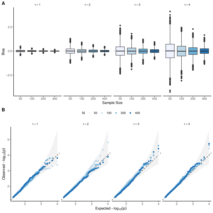
We first investigated the validity of our proposals through evaluation of the finite-sample bias, coverage probability of 95% confidence intervals (CIs), and type I error control in the absence of a treatment effect. Events were simulated from a homogeneous Poisson process with rate . Event-times were subject to independent censoring and the censoring time was generated from an exponential distribution with rate . A competing risk from death was also generated from an exponential distribution with rate . Data were simulated from two independent groups with a sample size per arm of for . The difference in AUMCFs was calculated with observation lengths of and results are summarized across 10,000 simulation replicates. Figure 1 demonstrates that estimation of the difference in AUMCFs shows minimal bias and that -values assessing the between group difference are uniformly distributed under the null. Numerical comparisons are presented in Table 1, which shows the type I error and coverage are near their nominal levels, while the empirical standard error (ESE) agrees closely asymptotic standard error (ASE). As expected, estimation precision decreases with increasing length of the observation period, .
| T1E Setting | Power Setting | ||||||
|---|---|---|---|---|---|---|---|
| Coverage (95% CI) | ASE | ESE | Coverage (95% CI) | ASE | ESE | ||
| 50 | 1 | 94.5 (94.0-94.9) | 0.116 | 0.116 | 93.9 (92.4-95.4) | 0.144 | 0.148 |
| 50 | 2 | 94.8 (94.4-95.2) | 0.338 | 0.338 | 94.2 (92.8-95.6) | 0.427 | 0.436 |
| 50 | 3 | 95.0 (94.5-95.4) | 0.647 | 0.648 | 94.5 (93.1-95.9) | 0.835 | 0.874 |
| 50 | 4 | 94.5 (94.0-94.9) | 1.041 | 1.056 | 94.0 (92.5-95.5) | 1.370 | 1.396 |
| 100 | 1 | 94.5 (94.0-94.9) | 0.082 | 0.083 | 94.0 (92.5-95.5) | 0.102 | 0.106 |
| 100 | 2 | 94.8 (94.4-95.3) | 0.241 | 0.241 | 93.7 (92.2-95.2) | 0.303 | 0.317 |
| 100 | 3 | 94.8 (94.4-95.3) | 0.461 | 0.469 | 95.0 (93.6-96.4) | 0.594 | 0.599 |
| 100 | 4 | 94.8 (94.4-95.3) | 0.742 | 0.749 | 95.1 (93.8-96.4) | 0.976 | 0.992 |
| 200 | 1 | 94.9 (94.5-95.3) | 0.058 | 0.059 | 95.9 (94.7-97.1) | 0.072 | 0.071 |
| 200 | 2 | 94.8 (94.3-95.2) | 0.170 | 0.172 | 93.5 (92.0-95.0) | 0.215 | 0.224 |
| 200 | 3 | 95.3 (94.8-95.7) | 0.327 | 0.327 | 94.7 (93.3-96.1) | 0.421 | 0.437 |
| 200 | 4 | 95.1 (94.6-95.5) | 0.528 | 0.532 | 94.9 (93.5-96.3) | 0.694 | 0.703 |
| 400 | 1 | 94.7 (94.3-95.2) | 0.041 | 0.042 | 94.9 (93.5-96.3) | 0.051 | 0.052 |
| 400 | 2 | 94.8 (94.3-95.2) | 0.121 | 0.122 | 95.2 (93.9-96.5) | 0.152 | 0.149 |
| 400 | 3 | 95.3 (94.9-95.7) | 0.232 | 0.229 | 94.2 (92.8-95.6) | 0.299 | 0.296 |
| 400 | 4 | 95.0 (94.6-95.4) | 0.374 | 0.374 | 94.5 (93.1-95.9) | 0.494 | 0.498 |
3.1 Power
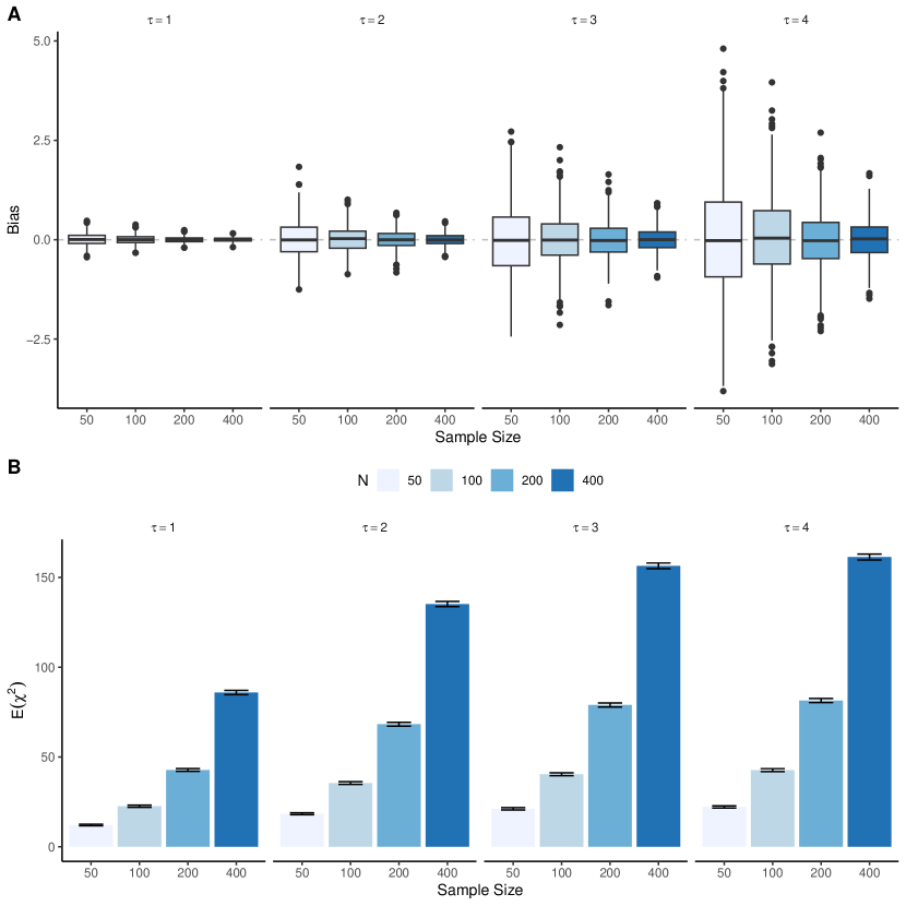
We next evaluated the performance of our proposed estimation and inference procedures for the AUMCF in the presence of a treatment effect. Data were simulated analogously to the null setting, but with the event rate in the treatment group set to and the event rate in the reference group as . The true treatment difference was estimated by averaging the difference in AUMCFs from a simulated trial with no censoring and a sample size of patients per arm across 2000 replicates. The results are summarized across 1,000 simulation replicates and are presented in Figure 2. Estimation of the treatment effect difference with the AUMCF exhibits minimal bias in the presence of a treatment effect across all sample sizes considered. Meanwhile, the power to detect a treatment difference increased, as expected, with both the sample size and the magnitude of the treatment difference. Note that the true treatment difference increases with a longer observation period because the event rate is constant in each arm, and twice as large in the reference group as in the treatment group.
3.2 Covariate Adjustment
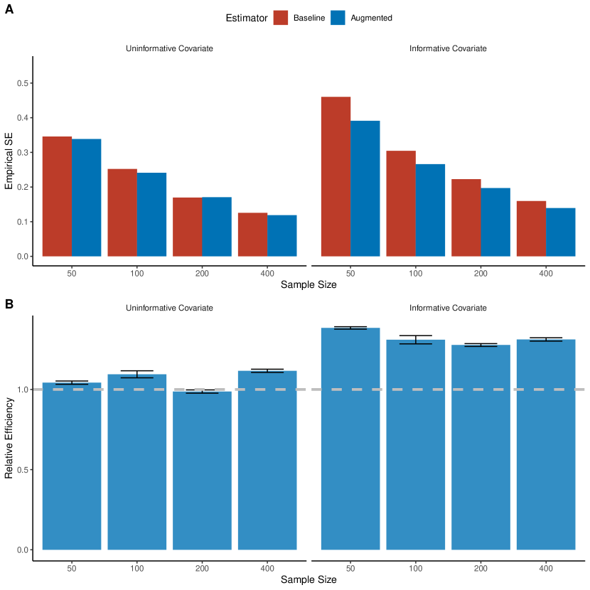
Lastly, we demonstrate the utility of augmenting the estimated difference in AUMCF with information in baseline covariates. For this simulation, we return to the null setting of no systematic difference in event rate between the treatment groups as the efficiency gain provided by augmentation does not depend on the presence or magnitude of a treatment effect. A continuous covariate was simulated for all subjects as . Two scenarios are considered, one in which the covariate is uninformative, having no effect on either the event or death rates, and a second in which it is informative. For the latter, each subject’s death rate was scaled by , where , and each subject’s event rate was scaled by , where . The results are presented in Figure 3 and based on 1,000 simulation replicates. As expected, augmentation with an uninformative covariate provided no benefit, with the 95% CIs for the relative efficiency including 1.0 in all cases, whereas augmentation with an informative covariate significantly improved efficiency. Different choices for led to qualitatively similar findings. The numerical results underlying Figure 3 are presented in Supplemental Tables 1-2.
4 Real data example
The Beta-Blocker Evaluation of Survival Trial (BEST) (Committee, 1995; Investigators et al., 2001) was a randomized, double-blinded, placebo-controlled clinical trial designed to evaluate whether bucindolol hydrochloride – a non-selective beta-adrenergic blocker and mild vasodilator – would improve overall survival (OS) among diverse patients with advanced heart failure (New York Heart Association [NYHA] classes III and IV) and reduced ejection fraction (LVEF ). A total of 2,708 eligible patients were randomized 1:1 to bucindolol or placebo. The primary endpoint was OS. There were multiple secondary endpoints, including the times to hospitalization (from heart failure or any cause), myocardial infarction, and heart transplantation. Based on an observed hazard ratio (HR) of 0.90 (95% CI, 0.78 to 1.02, ) for OS in the primary analysis, the study concluded there was no significant evidence of an OS benefit in the overall study population. Here we reanalyze primary data from the BEST trial not to reach different scientific conclusions, but to illustrate how to apply the methodology developed in this article.
Our data set includes 1,354 patients randomized to bucindolol and 1,353 randomized to placebo. For the primary endpoint of OS, there were 411 events in the bucindolol arm, and 448 events in the placebo arm. Kaplan-Meier (KM) estimates of the OS probability across 48 months of follow-up are presented in Supplemental Figure 1. The 48-month restricted mean survival time (RMST), which is the area under the Kaplan-Meier curve across the follow-up period, was 36.15 months for bucindolol and 35.10 months for placebo. This means that a heart failure patient randomized to bucindolol and followed for 48 months would expect to survive 36.15 months. The difference in 48-month RMSTs was 1.05 months (95% CI, -0.29 to 2.4 months, ) in favor of bucindolol.
OS may not capture disease burden as indicated for example by a hospitalization. We defined a composite disease-burden endpoint as the time to hospitalization from any cause, myocardial infarction, heart transplantation, and death, whichever occurred first. For this endpoint, there were 931 events in the bucindolol arm versus 971 in the palcebo arm. Kaplan-Meier curves for event-free survival across the 48 months of follow-up are presented in Supplemental Figure 2. The 48-month RMSTs were 19.1 months for bucindolol and 18.0 months for placebo. Here, the 19.1 months is interpreted as the expected event-free survival time of a patient randomized to bucindolol and scheduled for 48 months of follow-up. The difference in 48-month RMSTs was 1.16 months (95% CI, -0.21 to 2.5 months, ) in favor of bucindolol.
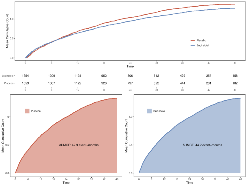
Time-to-first event analysis of the composite disease-burden endpoint does not take into account the clustering of events within patients, nor the fact that follow-up data beyond the first non-fatal event is often available. Specifically, for 825 patients in the bucindolol arm and 870 patients in the placebo arm, more than 1 unique event-time was available. We performed an AUMCF analysis on the composite endpoint, considering all occurrence a patient experienced. Here the patient-level counting process increments whenever an event included in the composite endpoint occurs, as opposed to upon recurrences of a single type of event (e.g., hospitalization), but the analysis of a multiple event-time endpoint (as considered here) otherwise proceeds identically to that of a recurrent event endpoint. The AUMCF analysis is illustrated in Figure 4. Across 48-months of follow-up, the AUMCFs were 44.2 months for bucindolol and 47.9 months for placebo. Note the important difference in interpretation compared with the RMST: the AUMCF is the expected event-free time lost across the follow-up period. Thus, a lower value is better. The difference in 48-month AUMCFs was 3.68 months (95% CI, 0.89 to 6.47 months, ) in favor of bucindolol. That is, across the 48 months of follow-up, patients randomized to bucindolol survived event-free (i.e., free of hospitalization, myocardial infarction, or heart transplanation) for an addition 3.68 months on average. Although all analyses presented thus far agree that patients receiving bucindolol tended to fare better, only the multiple event-time analysis reached statistical significance at the standard . Results from various sensitivity analyses are presented in the Supplemental Data Analyses, including an analysis based on the augmentation estimator with baseline covariates, and an analysis that excludes death from the composite disease-burden endpoint.
5 Discussion
In this paper, we have proposed a new estimand for quantifying treatment efficacy in comparative clinical studies with a multiple event endpoint: the area under the mean cumulative function (AUMCF). This area, which is interpreted as the expected total event-free time lost due to all event occurrences, aims to quantify the average patient’s cumulative disease burden across time. We demonstrated how to contrast the efficacy of two treatments by performing inference on the difference in AUMCFs. Terminal events are accounted for by stopping the counting process, allowing for assumption-free handling of competing risks. In contrast to existing methods for analyzing multiple or recurrent event data, the proposed difference of AUMCFs satisfies the two key properties for a population-level summary of the treatment difference outlined in McCaw et al. (2021), being both clinically interpretable and fully nonparametric.
However, our approach is not without limitations. If the terminal event rates differ substantially between treatment arms, then direct comparison of the MCFs or AUMCFs can be misleading. Indeed, a treatment that reduces mortality, but otherwise has no effect on the recurrence rate may actually increase the MCF and AUMCF by extending the time during which patients are at-risk to experience recurrences (McCaw et al., 2020). Furthermore, although we have implemented a nonparametric augmentation procedure to account for covariate differences between treatment groups, regression modeling to characterize the relationship between individual covariates and the AUMCF may be desirable, particularly in observational data settings. These regression models could be fit by means of inverse probability weighting or pseudo-values (Tian et al., 2014; Andersen and Perme, 2010). Future research in this direction is warranted, and will be conducted for future publications.
Acknowledgments
J. Gronsbell is grateful for support of an NSERC Discovery Grant (RGPIN-2021-03734).
References
- Andersen and Gill (1982) Andersen, P. K. and Gill, R. D. (1982). Cox’s regression model for counting processes: a large sample study. The Annals of Statistics pages 1100–1120.
- Andersen and Perme (2010) Andersen, P. K. and Perme, M. P. (2010). Pseudo-observations in survival analysis. Statistical Methods in Medical Research 19, 71 – 99.
- Austin et al. (2016) Austin, P. C., Lee, D. S., and Fine, J. P. (2016). Introduction to the analysis of survival data in the presence of competing risks. Circulation 9, 601 – 609.
- Claggett et al. (2018) Claggett, B., Tian, L., Fu, H., Solomon, S. D., and Wei, L.-J. (2018). Quantifying the totality of treatment effect with multiple event-time observations in the presence of a terminal event from a comparative clinical study. Statistics in Medicine 37, 3589–3598.
- Claggett et al. (2022) Claggett, B. L., McCaw, Z. R., Tian, L., McMurray, J. J. V., Jhund, P. S., Uno, H., et al. (2022). Quantifying treatment effects in trials with multiple event-time outcomes. NEJM Evidence 1, 10.1056/evidoa2200047.
- Committee (1995) Committee, B. S. (1995). Design of the beta-blocker evaluation survival trial (best). American Journal of Cardiology 75, 1220 – 1223.
- Cook and Lawless (1997) Cook, R. J. and Lawless, J. F. (1997). Marginal analysis of recurrent events and a terminating event. Statistics in Medicine 16, 911–924.
- Ghosh and Lin (2000) Ghosh, D. and Lin, D. (2000). Nonparametric analysis of recurrent events and death. Biometrics 56, 554–562.
- Ghosh and Lin (2002) Ghosh, D. and Lin, D. Y. (2002). Marginal regression models for recurrent and terminal events. Statistica Sinica pages 663–688.
- Glynn and Buring (2001) Glynn, R. J. and Buring, J. E. (2001). Counting recurrent events in cancer research.
- Gregson et al. (2023) Gregson, J., Stone, G. W., Bhatt, D. L., Packer, M., Anker, S. D., Zeller, C., et al. (2023). Recurrent events in cardiovascular trials: Jacc state-of-the-art review. Journal of the American College of Cardiology 82, 1445 – 1463.
- Huang and Wang (2004) Huang, C.-Y. and Wang, M.-C. (2004). Joint modeling and estimation for recurrent event processes and failure time data. Journal of the American Statistical Association 99, 1153–1165.
- Investigators et al. (2001) Investigators, B.-B. E. o. S. T., Eichhorn, E. J., Domanski, M. J., Krause-Steinrauf, H., Bristow, M. R., and Lavori, P. W. (2001). A trial of the beta-blocker bucindolol in patients with advanced chronic heart failure. New England Journal of Medicine 344, 1659 – 1667.
- Lawless (1987) Lawless, J. F. (1987). Regression methods for poisson process data. Journal of the American Statistical Association 82, 808–815.
- Lawless and Nadeau (1995) Lawless, J. F. and Nadeau, C. (1995). Some simple robust methods for the analysis of recurrent events. Technometrics 37, 158–168.
- Li and Lagakos (1997) Li, Q. H. and Lagakos, S. W. (1997). Use of the wei–lin–weissfeld method for the analysis of a recurring and a terminating event. Statistics in Medicine 16, 925–940.
- Lin et al. (2000) Lin, D. Y., Wei, L.-J., Yang, I., and Ying, Z. (2000). Semiparametric regression for the mean and rate functions of recurrent events. Journal of the Royal Statistical Society: Series B (Statistical Methodology) 62, 711–730.
- McCaw et al. (2022) McCaw, Z. R., Claggett, B. L., Tian, L., Solomon, S. D., Berwanger, O., Pfeffer, M. A., et al. (2022). Practical recommendations on quantifying and interpreting treatment effects in the presence of terminal competing risks: A review. JAMA Cardiology 7, 450 – 456.
- McCaw et al. (2019) McCaw, Z. R., Orkaby, A. R., Wei, L.-J., Kim, D. H., and Rich, M. W. (2019). Applying evidence-based medicine to shared decision making: Value of restricted meansurvival time. The American Journal of Medicine 132, 13 – 15.
- McCaw et al. (2020) McCaw, Z. R., Tian, L., Sheth, K. N., Hsu, W.-T., Kimberly, W. T., and Wei, L.-J. (2020). Selecting appropriate endpoints for assessing treatment effects in comparative clinical studies for covid-19. Contemporary Clinical Trials 97, 106145.
- McCaw et al. (2021) McCaw, Z. R., Tian, L., Wei, J., Claggett, B. L., Bretz, F., Fitzmaurice, G., et al. (2021). Choosing clinically interpretable summary measures and robust analytic procedures for quantifying the treatment difference in comparative clinical studies. Statistics in Medicine 40, 6235 – 6242.
- Mogensen et al. (2018) Mogensen, U. M., Gong, J., Jhund, P. S., Shen, L., Køber, L., Desai, A. S., et al. (2018). Effect of sacubitril/valsartan on recurrent events in the prospective comparison of arni with acei to determine impact on global mortality and morbidity in heart failure trial (paradigm-hf). European Journal of Heart Failure 20, 760–768.
- Pepe and Cai (1993) Pepe, M. S. and Cai, J. (1993). Some graphical displays and marginal regression analyses for recurrent failure times and time dependent covariates. Journal of the American Statistical Association 88, 811–820.
- Pfeffer et al. (2022) Pfeffer, M. A., Claggett, B., Lewis, E. F., Granger, C. B., Køber, L., Maggioni, A. P., et al. (2022). Impact of sacubitril/valsartan versus ramipril on total heart failure events in the paradise-mi trial. Circulation 145, 87–89.
- Prentice et al. (1981) Prentice, R. L., Williams, B. J., and Peterson, A. V. (1981). On the regression analysis of multivariate failure time data. Biometrika 68, 373–379.
- Robins et al. (1994) Robins, J. M., Rotnitzky, A., and Zhao, L. P. (1994). Estimation of regression coefficients when some regressors are not always observed. Journal of the American Statistical Association 89, 846–866.
- Rogers et al. (2012) Rogers, J. K., McMurray, J. J., Pocock, S. J., Zannad, F., Krum, H., van Veldhuisen, D. J., et al. (2012). Eplerenone in patients with systolic heart failure and mild symptoms: analysis of repeat hospitalizations. Circulation 126, 2317–2323.
- Rogers et al. (2014) Rogers, J. K., Pocock, S. J., McMurray, J. J., Granger, C. B., Michelson, E. L., Östergren, J., et al. (2014). Analysing recurrent hospitalizations in heart failure: a review of statistical methodology, with application to charm-preserved. European Journal of Heart Failure 16, 33–40.
- Solomon et al. (2018) Solomon, S. D., Rizkala, A. R., Lefkowitz, M. P., Shi, V. C., Gong, J., Anavekar, N., et al. (2018). Baseline characteristics of patients with heart failure and preserved ejection fraction in the paragon-hf trial. Circulation: Heart Failure 11, e004962.
- Sparapani et al. (2020) Sparapani, R. A., Rein, L. E., Tarima, S. S., Jackson, T. A., and Meurer, J. R. (2020). Non-parametric recurrent events analysis with bart and an application to the hospital admissions of patients with diabetes. Biostatistics 21, 69–85.
- Tian et al. (2012) Tian, L., Cai, T., Zhao, L., and Wei, L.-J. (2012). On the covariate-adjusted estimation for an overall treatment difference with data from a randomized comparative clinical trial. Biostatistics 13, 256–273.
- Tian et al. (2014) Tian, L., Zhao, L., and Wei, L.-J. (2014). Predicting the restricted mean event time with the subject’s baseline covariates in survival analysis. Biostatistics 15, 222–233.
- Tsiatis et al. (2008) Tsiatis, A. A., Davidian, M., Zhang, M., and Lu, X. (2008). Covariate adjustment for two-sample treatment comparisons in randomized clinical trials: a principled yet flexible approach. Statistics in medicine 27, 4658–4677.
- Uno et al. (2014) Uno, H., Claggett, B., Tian, L., Inoue, E., Gallo, P., Miyata, T., et al. (2014). Moving beyond the hazard ratio in quantifying the between-group difference in survival analysis. Journal of Clinical Oncology 32, 2380 – 2385.
- Wang et al. (2001) Wang, M.-C., Qin, J., and Chiang, C.-T. (2001). Analyzing recurrent event data with informative censoring. Journal of the American Statistical Association 96, 1057–1065.
- Wei et al. (1989) Wei, L.-J., Lin, D. Y., and Weissfeld, L. (1989). Regression analysis of multivariate incomplete failure time data by modeling marginal distributions. Journal of the American Statistical Association 84, 1065–1073.
Supporting information
R package. MCC, developed for the proposed method is available at https://github.com/zrmacc/MCC.
R Code. Code used to produce the simulation and data analysis results is available at https://github.com/Kxsssss/AUMCF_Sim.