Application of quantum annealing for scalable robotic assembly line optimization: a case study

Abstract

The even distribution and optimization of tasks across resources and workstations is a critical process in manufacturing aimed at maximizing efficiency, productivity, and profitability, known as Robotic Assembly Line Balancing (RALB). With the increasing complexity of manufacturing required by mass customization, traditional computational approaches struggle to solve RALB problems efficiently. To address these scalability challenges, we investigate applying quantum computing, particularly quantum annealing, to the real-world based problem. We transform the integer programming formulation into a quadratic unconstrained binary optimization problem, which is then solved using a hybrid quantum-classical algorithm on the D-Wave Advantage 4.1 quantum computer. In a case study, the quantum solution is compared to an exact solution, demonstrating the potential for quantum computing to enhance manufacturing productivity and reduce costs. Nevertheless, limitations of quantum annealing, including hardware constraints and problem-specific challenges, suggest that continued advancements in quantum technology will be necessary to improve its applicability to RALB manufacturing optimization.

I Introduction

Robotic Assembly Line Balancing (RALB) is crucial for maximizing production efficiency, productivity, and profitability [1]. It involves assigning tasks among workstations to optimize production time or workstation count, considering automated resources and alternatives [2]. An optimal line balance is essential for today’s manufacturing companies to meet customer demands while maintaining competitiveness [3]. With increasing manufacturing complexity due to mass customization, traditional approaches face scalability challanges and struggle to solve the Robotic Assembly Line Balancing Problems (RALBPs) efficiently [4, 5].

Quantum computing shows promising results in addressing these scalability challenges, potentially enabling near-optimal or faster optimal solutions for RALBP [6, 7]. Quantum algorithms like Quantum Approximate Optimization Algorithm (QAOA) [8], and quantum annealing [9] have shown promising results in solving different optimization problems [10, 11], making them appealing for the RALBP.

We investigate the potential of quantum computing for RALBP, scrutinizing the approach to address scalability challenges by translating the Integer Programming (IP) problem into a Quadratic Unconstrained Binary Optimization (QUBO) and mapping it to an Ising model. We solve a problem instance on the D-Wave Advantage 4.1 quantum computer to identify potentials and problems. In this use case study, we compare a quantum approach to classical methods for solving the RALBP, assessing their practical benefits in real-world manufacturing scenarios. By detailing the procedure to address the problem with quantum computing and providing a corresponding python tool [12], we aim at enabling manufacturers to assess the potential of quantum computing for the RALBP.

The remainder of this paper is structured as follows. In Section II, the current state of the art of solving the RALBP as well as the application of quantum computing to combinatorial optimization problems (COPs) is discussed. Section III presents the IP and the QUBO model formulation, and the quantum annealing solution approach. A RALBP case study is presented in Section IV, and Section V discusses the results and provides an outlook.

II Related Work

The definition of the RALBP, is driven by real-world manufacturing needs for flexibility and increased competitiveness through specialized production equipment [2]. Classical methods for solving the RALBP include exact methods [13], heuristics [14, 15] and meta-heuristic approaches [16, 17], with significant improvements in the last decades [18]. However, these methods often struggle when dealing with large-scale and highly complex instances [19]. Either they provide high-quality results for small instances through exact solution techniques [20], or scalability in complex instances with reduced quality through meta-heuristic techniques [16]. As the number of tasks and workstations increases, the computational complexity proves a significant issue due to the NP-hard problem type, making it infeasible to find optimal solutions within a reasonable time. This scalability issue has motivated the exploration of new computational paradigms, such as quantum computing, to tackle the RALBP more efficiently.

Recently, the availability of early-stage quantum computing devices has raised interest in applying quantum algorithms to a wide range of problems. Alongside the simulation of physical systems and machine learning, COPs has been one of the areas of research where quantum computing has been applied [10]. Quantum annealing, a specialized form of quantum computation, is naturally suited for solving COPs [21]. It returns the lowest possible energy in a physical system described by the Ising Hamiltonian, which corresponds to the optimal solution of the COP. Quantum annealers are already commercially available and have been applied to various industrial problems [22, 23].

Quantum annealing has shown promising results in manufacturing, including layout planning [19], job shop scheduling [24], and production planning [4]. A list of industry-related reference problems suitable for quantum computing in the automotive industry has been curated [25], with some already being addressed [26]. Benefits of quantum annealing in manufacturing include handling complex combinatorial problems, potentially finding higher-quality solutions, or faster solution generation for certain problems [25, 21, 6]. However, limited qubit counts, connectivity issues, and noise in quantum systems currently restrict its universal applicability.

III Methods

In this section, we introduce the IP model for the RALBP. This is then used to reformulate the problem in a QUBO form which allows for a solution with a quantum computer.

III.1 Integer Programming Model Formulation

The RALBP aims to assign tasks to production equipment and allocate equipment to workstations to manufacture a desired product. An assignment optimization can maximize efficiency or minimize investment costs. Manufacturing requires all tasks to be assigned, each with equipment-specific processing times, following a predetermined assembly order within a given cycle time. The pieces of equipment are selected from available production resources. The IP model formulation requires two binary decision variables, one for the assignment of equipment to workstations and the second for the assignment of tasks to workstations. We define $y_{jk}=1$ if equipment $j$ is assigned to workstation $k$, $0$ otherwise. Additionally, $x_{ijk}=1$ if task $i$ is performed by equipment $j$ at workstation $k$, $0$ otherwise. An overview of the variable notation for the RALBP model is given in Table 1.

This results in the IP problem formulation for the RALBP [2]:

$$\min\sum_{j=1}^{r}\sum_{k=1}^{m}c_{j}y_{jk}$$ (1)

s.t.

$$\sum_{j=1}^{r}\sum_{k=1}^{m}x_{ijk}=1 \forall i$$ (2)

$$\sum_{i=1}^{n}t_{ij}x_{ijk}\leq Cy_{jk} \forall j,k$$ (3)

$$\sum_{i=1}^{n}\sum_{j=1}^{r}t_{ij}x_{ijk}\leq C \forall k$$ (4)

$$\sum_{j=1}^{r}\sum_{k=1}^{m}kx_{pjk}\leq\sum_{j=1}^{r}\sum_{l=1}^{m}lx_{ijl} \forall p\in\mathcal{P}_{i},i$$ (5)

The objective function (1) minimizes total equipment costs. Constraint (2) assigns each task to exactly one workstation. Constraint (3) ensures that the task time at each piece of equipment does not exceed cycle time and that pieces of equipment can only perform tasks if assigned to the workstation. Additionally, multiple pieces of equipment can be assigned to one workstation. The sum of the total workstation task time is limited to cycle time by constraint (4). Constraint (5) enforces task precedence graph relations given by edges $\mathcal{E}=\{(p,i)\,|\,p\in\mathcal{P}_{i},i\in[1,n]\}$, where task $p$ precedes task $i$.

Table 1: Variable description and overview for the Integer Programming model.

Variable name	Variable description
$n$	Number of tasks.
$r$	Number of equipment.
$m$	Number of workstations.
$i$	Task index, $i\in\{1,\dots,n\}$.
$j$	Equipment index, $j\in\{1,\dots,r\}$.
$k$	Workstation index, $k\in\{1,\dots,m\}$.
$t_{ij}$	Processing time of task $i$ when performed by equipment $j$, in s.
$C$	Cycle time, in s.
$c_{j}$	Cost of equipment $j$, in $.
$\mathcal{P}_{i}$	The set of tasks which precede task $i$.

III.2 Quadratic Unconstrained Binary Optimization

To solve the RALBP with quantum computing, the problem needs to be formulated as a QUBO. QUBO is a problem class that is capable of representing a wide range of COPs as minimization problems of the general form

$$\min_{x\in\{0,1\}^{n}}x^{\intercal}Qx\,,$$ (6)

with the $n$-dimensional decision vector $x$ and the quadratic QUBO-Matrix $Q$ [27]. In the case of the RALBP, the optimization problem is formulated as a linear integer program with constraints, which gets transformed with the following steps.

First, the linear cost function of the RALBP in Eq. (1) can be easily transformed to a quadratic one for the binary case because the equality $x=x^{2}$ holds for $x\in\{0,1\}$. Second, equality constraints of the form $Ax=b$ can be reformulated and added to the quadratic cost function as

$$\min_{x\in\{0,1\},Ax=b}x^{\intercal}Qx=\min_{x\in\{0,1\}}x^{\intercal}Qx+\lambda\left(Ax-b\right)^{2}\,,$$ (7)

with help of Lagrange-parameters $\lambda$. In the case of the RALBP, four Lagrange parameters are added, one for each constraint. This transformation changes the hard constraints of the original problem formulation to soft constraints. Third, inequality constraints can be transformed into equality constraints, as in $Ax\leq b\Leftrightarrow Ax+s=b,s>0$, by introducing slack variables $s$. Technically, the slack variables are implemented as decision variables with weights that can produce values between $0$ and $b$, i. e., the binary representation of $b$. Their use increases the problem size significantly. The amount of additional decision variables are determined by the binary representation. In total, these transformations introduce $n_{s}=(r+rm)\lceil\log_{2}(C)\rceil+\absolutevalue{\mathcal{E}}\lceil\log_{2}(nrm)\rceil$ new variables. The first term originates from the two inequality constraints Eq. (3) and Eq. (4) that include the cycle time $C$ in the original formulation. The second term stems from the inequality constraint Eq. (5) of the precedence graph, with $\absolutevalue{\mathcal{E}}$ the number of edges. To reduce the total number of decision variables, rescaling the cycle time $C$ and all the task times $t_{i}$ by dividing by their greatest common divisor is advisable. Additionally, one only needs to consider the tasks assigned to machines permitted by $t_{ij}$ to reduce the number of decision variables needed. The transformation process also requires fixing the number of workstations $m$ to yield a constant QUBO size.

To automatically transform the RALBP into a QUBO representation, we have developped a python library which is available in GitLab [12]. The library allows the formulation of arbitrary RALBP instances and their corresponding QUBO representations, which then can be solved with any available QUBO solver.

III.3 Quantum Annealing

The QUBO problem can be mapped onto a physical model describing interacting qubits called Ising model. Finding the ground state of this model is then equivalent to solving the QUBO. The Ising model is given by the Hamiltonian

$$H_{\text{Ising}}=-\sum_{i<j}J_{ij}\hat{\sigma}^{z}_{i}\hat{\sigma}^{z}_{j}-\sum_{j}h_{j}\hat{\sigma}^{z}_{j}\,.$$ (8)

Here, $\hat{\sigma}^{z}_{j}$ is the Pauli $Z$-operator that describes the state of qubit $j$ in the computational basis. The terms $J_{ij}$ and $h_{j}$ correspond to the interaction strength between qubits and an external field. This Hamiltonian can be directly implemented on a quantum computer, making the problem susceptible to a variety of algorithms designed to find a system’s minimum energy configuration.

To map Eq. (6) onto Eq. (8), we apply the transformation $\hat{\sigma}^{z}_{j}=1-2x_{j}$. The diagonal elements $Q_{jj}$ of the QUBO-matrix in Eq. (6) are identified with the linear terms $h_{j}$ in Eq. (8) while the off-diagonal elements $Q_{ij}(i\neq j)$ are mapped onto $J_{ij}$. Constant terms do not affect the optimal solution and are thus omitted. Several quantum algorithms can be used to determine the ground state of Eq. (8) [8, 9]. Here, we focus on quantum annealing, which allows for slightly larger problem sizes than algorithms implemented on gate-based quantum computers. The algorithm initializes the system in the ground state of a well-known and easily preparable Hamiltonian, then adjusts parameters to prepare the problem-encoding Hamiltonian Eq. (8). If done slowly, the system will remain in the ground state. However, quantum annealing implementations do not exclusively produce the lowest energy state but rather a probability distribution biased toward that state. Sampling is then used to obtain near-optimal solutions for the QUBO problem.

The algorithm is implemented using the D-Wave’s Advantage 4.1 quantum processing unit (QPU), with over $5,\!000$ qubits, coupling each qubit with $15$ other [28]. Here, each spin variable $\hat{\sigma}_{j}^{z}$ of the Ising Hamiltonian is mapped to a superconducting qubit on a lattice graph, and couplers implement interactions between qubits. Mapping the full Ising Hamiltonian directly to the QPU leads to long chains of redundant qubits, which are prone to noise. Therefore, we utilize the hybrid quantum-classical algorithm QBSolv [29], combining partitioning of the QUBO-matrix and the heuristic Tabular-search algorithm. The smaller sub-QUBOs are solved using the D-Wave annealer. This approach also allows solving larger instances of QUBO problems.

III.4 Lagrange Parameter Search

Introducing Lagrange parameters in Eq. (7) requires additional hyperparameter optimization. These parameters balance the constraints’ influence on the solution cost and their respective importance. Their choice is highly problem-dependent and significantly affects solution quality. If chosen too small, sampling could have a bias towards infeasible solutions; if chosen too large, suboptimal solutions may predominate. A grid search is performed to find the optimal Lagrange parameters. For each combination, the QUBO is sampled $1,\!000$ times, selecting the combination with the highest number of optimal solutions. A solution is considered optimal if it is valid, i. e., all constraints are satisfied, and the cost equals the global minimum of the RALBP. To limit QPU execution time, we use simulated annealing from the dwave-neal package [30] instead of direct quantum computer execution. Simulated annealing is a classical algorithm, approximating global optima through probabilistic neighborhood search [31]. Using this algorithm here is reasonable because both quantum and classical annealing operate on the same cost landscape. We assume that 1) an energy landscape that is favorable for simulated annealing benefits also quantum annealing, and 2) real quantum hardware errors are minor compared to Lagrange parameter modifications.

IV Case Study

This section introduces a simple RALBP case study on which the quantum annealing solution and the classical IP model are compared.

IV.1 Data Description

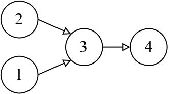
Figure 1: Precedence graph for the case study with $4$ tasks.

We consider a reduced complexity RALBP with four tasks across two workstations and two equipment types. In the task matrix $t_{ij}$, $-1$ indicates inability to perform a specific task. The task matrix $t_{ij}$ and cost vector $c_{j}$ are defined as

$$t_{ij}=\begin{pmatrix}8&-1\\ 13&14\\ 18&-1\\ 15&20\end{pmatrix}\qquad c_{j}=\begin{pmatrix}100,\!000\\ 60,\!000\end{pmatrix}\,.$$

Finally, the directed precedence graph for the case study with $4$ tasks is shown in Figure 1, defining predecessor and successor relationships. The cycle time constraint is set to $C=40$.

IV.2 Results

The optimal assignment to the case study by an exact solution to the IP model results in the task to equipment and workstation assignment shown in Table 2. The solution took $0.03\,\text{s}$ computation time.

Table 2: The $C=40$ example took $0.03\,\text{s}$ computation time with an objective value of $160,\!000$, and $2$ pieces of equipment in $2$ workstations.

Cycle time	Workstation	Equipment	Tasks	Processing times	Workstation time
$C=40$	$k=1$	$j=1$	$i=\{1,2,3\}$	$\{t_{11}=8,t_{12}=13,t_{13}=18\}$	$39$
	$k=2$	$j=2$	$i=\{4\}$	$\{t_{24}=20\}$	$20$

The formulation as a QUBO yields a quadratic matrix of dimension $64\times 64$, i. e., a problem with $64$ binary decision variables which can be encoded using $64$ qubits.

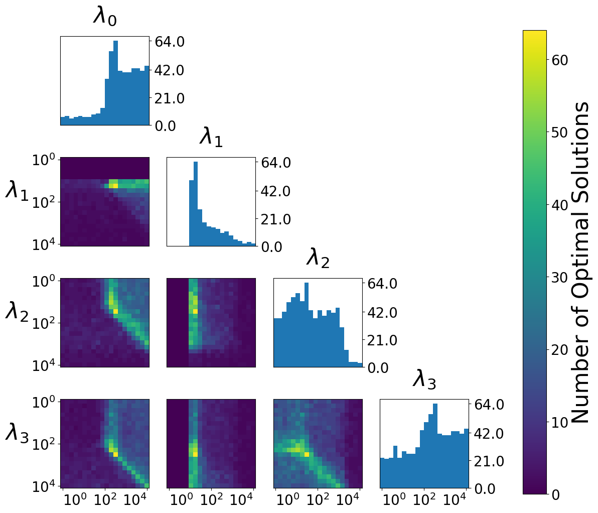
Figure 2: Number of optimal solutions for each fixed combination of Lagrange parameters in Eq. (7) out of $1,\!000$ samples with dwave-neal simulated annealer. The plots on the diagonal show the maximal number of optimal solutions for a single fixed Lagrange parameter aggregated over all combinations of the other Lagrange parameters. The plots on the lower triangle show the maximal number of optimal solutions for two fixed Lagrange parameters. The set of optimal Lagrange parameters for our case study with $C=40$ are $\lambda_{1}=335.982$, $\lambda_{2}=18.330$, $\lambda_{3}=29.764$, $\lambda_{4}=335.982$.

Figure 2 shows the search space and the results of the Lagrange parameter search from Subsection III.4. Each row and column corresponds to a Lagrange parameter $\lambda_{i}$. The histograms on the diagonal and the heatmaps on the lower triangle show the maximum number of occurrences when one or two Lagrange parameters are fixed. While many configurations of Lagrange parameters can produce an optimal solution, there is a clear spike in the number of occurrences of the optimal solution visible in the histograms on the diagonal and the heatmaps on the lower triangle.

Using the optimal Lagrange parameters detailed in Figure 2, we obtain $64$ optimal solutions out of $1,\!000$ samples with the dwave-neal simulated annealer. Sampling $1,\!000$ solutions with dwave-neal took $4.3\,\text{s}$.

(a) Occurrence of 50 most frequent solutions

(b) Cost of 50 most frequent solutions

Figure 3: Top $50$ samples out of $1,\!000$ produced by QBSolv with a D-Wave Advantage System 4.1 quantum annealer. Each bar represents one unique solution. The color and pattern of the bar are determined by whether the according solution is valid, i. e., fulfills all constraints Eqs. (2)-(5). In LABEL:sub@fig:dwave-results:a, the height of the bar shows the number of occurrences of the solution. In LABEL:sub@fig:dwave-results:b, the height of the bar shows the cost according to the original cost function in Eq. (1). The optimal cost value is also highlighted as a yellow line in LABEL:sub@fig:dwave-results:b.

For the selected set of Lagrange parameters, we further run the QBSolv algorithm on the D-Wave Advantage 4.1 QPU, sampling $1,\!000$ solutions. This sampling took a total computation time of $10,\!110.5\,\text{s}$, including the communication with the QPU but excluding the computation of the Lagrange parameters, which are assumed to be known.

Figure 3a shows the $50$ most occurring solutions, ordered by occurrence and color-coded according to the validity of the solution. Figure 3b shows the according cost value from Eq. (1). Additionally, the optimal cost value, i. e., the cost value of the best possible solution, as obtained by the IP solution, is marked in the plot.

Within the $50$ most occurring samples, there are $32$ valid solutions and $18$ invalid solutions. Multiple optimal solutions are also occurring among the $50$ most occurring solutions. The first optimal solution is in the seventh position and occurs $12$ times. The $50$ most occurring samples contain $34$ occurrences of $4$ different configurations of an optimal solution.

Comparing the results from simulated and quantum annealing, we find that simulated annealing produces a larger number of optimal solutions than quantum annealing. This is expected because quantum computers are subject to hardware noise and short coherence times, which ultimately require a trade-off between non-adiabatic errors if the annealing time is too fast and decoherence errors if it is too slow.

V Discussion

This work investigated the applicability of quantum annealing to the manufacturing optimization problem of RALB to counteract the ever-increasing complexity in production domains, where traditional approaches struggle to solve problems efficiently. A software toolbox was developed and published to transform the optimization instances into a QUBO formulation, making it solvable using quantum algorithms such as quantum annealing. To avoid limitations of currently available quantum computers, a hybrid quantum-classical approach using QBSolv in combination with a D-Wave Advantage 4.1 system QPU was used to produce sample solutions.

We evaluated the application on a RALBP case study instance, which was first transformed to a QUBO representation with the developed toolbox and then solved. The results were compared to the classical IP formulation and the simulated annealing algorithm. All methods found the optimal solution, with the traditional IP solution being the fastest. Quantum annealing produced slightly less feasible solutions than simulated annealing. However, simulated annealing is expected to get stuck more easily in local minima, which are more frequent with larger instances, ultimately hindering the scalability. We point out that although we report and discuss execution times on our use case, a speed-up in computation time is neither the primary goal of this work nor to be expected in this problem instance. The central premise is scaling advantages that might be harvested in larger instances. However, the current state of quantum computing hardware limits the size of problems that can be investigated. The low connectivity of the qubits within the quantum computer requires the use of ancillary qubits, which results in larger errors. Ultimately, these errors currently limit the applicability to larger-scale RALBP instances, which is why the current study is limited to this small use case. With further progress of the quantum hardware, both problems could be mitigated by removing the need for the search-based hybrid algorithm and enabling the application to larger-scale RALBPs where a scaling benefit is expected. We thus present the results on a small instance as a step towards scalability, providing researchers with a starting point that includes the QUBO-transformation library, the showcased approach, and instance evaluation. This foundation aims to enable future advancements in the field as quantum hardware continues to evolve and improve, ultimately leading to improved productivity and efficiency in manufacturing.

A significant benefit of using a sampling-based approach is the availability of multiple valid solutions rather than one, offsetting the computation time and, thus, scalability. These solutions can be leveraged for metrics other than the original cost function without additional effort, i. e., no further sampling for more solutions is required. A limitation of this approach is that the number of workstations has to be fixed for formulating the QUBO. The choice regarding the predefined number of workstations must be conservative, providing enough workstations to produce a feasible solution, potentially requiring more qubits than are ultimately necessary. Heuristics could provide a guided estimation for certain properties, such as the number of workstations.

Future investigations could include multi-objective optimization, leveraging the solution sampling for multiple production goals. In general, the presented approach is promising for the manufacturing problem of RALB if quantum annealing hardware advances to a point where it can be used efficiently for the full QUBO formulation. Also, other quantum optimization approaches using gate-based quantum computers could lead to better results when more mature, especially fully fault-tolerant, quantum hardware is available.

References

- Becker and Scholl [2006] C. Becker and A. Scholl, A survey on problems and methods in generalized assembly line balancing, European Journal of Operational Research 168, 694 (2006).
- Rubinovitz et al. [1993] J. Rubinovitz, J. Bukchin, and E. Lenz, Ralb - a heuristic algorithm for design and balancing of robotic assembly lines, CIRP Annals - Manufacturing Technology 42, 497 (1993).
- Touzout and Benyoucef [2019] F. A. Touzout and L. Benyoucef, Multi-objective sustainable process plan generation in a reconfigurable manufacturing environment: Exact and adapted evolutionary approaches, International Journal of Production Research 57, 2531 (2019).
- Riandari et al. [2021] F. Riandari, A. Alesha, and H. T. Sihotang, Quantum computing for production planning, International Journal of Enterprise Modelling 15, 163 (2021).
- Boysen et al. [2022] N. Boysen, P. Schulze, and A. Scholl, Assembly line balancing: What happened in the last fifteen years?, European Journal of Operational Research 301, 797 (2022).
- Luckow et al. [2021] A. Luckow, J. Klepsch, and J. Pichlmeier, Quantum Computing: Towards Industry Reference Problems, Digitale Welt 5, 38 (2021).
- Pirnay et al. [2024] N. Pirnay, V. Ulitzsch, F. Wilde, J. Eisert, and J.-P. Seifert, An in-principle super-polynomial quantum advantage for approximating combinatorial optimization problems via computational learning theory, Science Advances 10, eadj5170 (2024).
- Farhi et al. [2014] E. Farhi, J. Goldstone, and S. Gutmann, A quantum approximate optimization algorithm (2014), arXiv:1411.4028 [quant-ph] .
- Finnila et al. [1994] A. Finnila, M. Gomez, C. Sebenik, C. Stenson, and J. Doll, Quantum annealing: A new method for minimizing multidimensional functions, Chemical Physics Letters 219, 343 (1994).
- Abbas et al. [2023] A. Abbas, A. Ambainis, B. Augustino, A. Bärtschi, H. Buhrman, C. Coffrin, G. Cortiana, V. Dunjko, D. J. Egger, B. G. Elmegreen, N. Franco, F. Fratini, B. Fuller, J. Gacon, C. Gonciulea, S. Gribling, S. Gupta, S. Hadfield, R. Heese, G. Kircher, T. Kleinert, T. Koch, G. Korpas, S. Lenk, J. Marecek, V. Markov, G. Mazzola, S. Mensa, N. Mohseni, G. Nannicini, C. O’Meara, E. P. Tapia, S. Pokutta, M. Proissl, P. Rebentrost, E. Sahin, B. C. B. Symons, S. Tornow, V. Valls, S. Woerner, M. L. Wolf-Bauwens, J. Yard, S. Yarkoni, D. Zechiel, S. Zhuk, and C. Zoufal, Quantum optimization: Potential, challenges, and the path forward (2023), arXiv:2312.02279 [quant-ph] .
- King et al. [2023] A. D. King, J. Raymond, T. Lanting, R. Harris, A. Zucca, F. Altomare, A. J. Berkley, K. Boothby, S. Ejtemaee, C. Enderud, E. Hoskinson, S. Huang, E. Ladizinsky, A. J. R. MacDonald, G. Marsden, R. Molavi, T. Oh, G. Poulin-Lamarre, M. Reis, C. Rich, Y. Sato, N. Tsai, M. Volkmann, J. D. Whittaker, J. Yao, A. W. Sandvik, and M. H. Amin, Quantum critical dynamics in a 5,000-qubit programmable spin glass, Nature 617, 61 (2023).
- Willmann [2024] M. Willmann, ALB QUBO (version 1.0.0) (2024).
- Li et al. [2020] Z. Li, I. Kucukkoc, and Q. Tang, A comparative study of exact methods for the simple assembly line balancing problem, Soft Computing 24, 11459 (2020).
- Zhang et al. [2018] Y. Zhang, X. Hu, and C. Wu, Heuristic algorithm for type ii two-sided assembly line rebalancing problem with multi-objective, in MATEC Web of Conferences, Vol. 175 (2018) p. 03063.
- Borba et al. [2018] L. Borba, M. Ritt, and C. Miralles, Exact and heuristic methods for solving the robotic assembly line balancing problem, European Journal of Operational Research 270, 146 (2018).
- Albus et al. [2024] M. Albus, T. Hornek, W. Kraus, and M. F. Huber, Towards scalability for resource reconfiguration in robotic assembly line balancing problems using a modified genetic algorithm, Journal of Intelligent Manufacturing 10.1007/s10845-023-02292-0 (2024).
- Manavizadeh et al. [2012] N. Manavizadeh, M. Rabbani, D. Moshtaghi, and F. Jolai, Mixed-model assembly line balancing in the make-to-order and stochastic environment using multi-objective evolutionary algorithms, Expert Systems with Applications 39, 12026 (2012).
- Chutima [2022] P. Chutima, A comprehensive review of robotic assembly line balancing problem, Journal of Intelligent Manufacturing 33, 1 (2022).
- Klar et al. [2022] M. Klar, P. Schworm, X. Wu, M. Glatt, and J. C. Aurich, Quantum Annealing based factory layout planning, Manufacturing Letters 32, 59 (2022).
- Dolgui and Ihnatsenka [2009] A. Dolgui and I. Ihnatsenka, Branch and bound algorithm for a transfer line design problem: Stations with sequentially activated multi-spindle heads, European Journal of Operational Research 197, 1119 (2009).
- Yarkoni et al. [2022] S. Yarkoni, E. Raponi, T. Bäck, and S. Schmitt, Quantum annealing for industry applications: Introduction and review, Reports on Progress in Physics 85, 104001 (2022).
- Cohen and Tamir [2014] E. Cohen and B. Tamir, D-Wave and predecessors: From simulated to quantum annealing, International Journal of Quantum Information 12, 1430002 (2014).
- Liu and Li [2021] Z. Liu and S. Li, A Quantum Computing Based Numerical Method for Solving Mixed-Integer Optimal Control Problems, Journal of Systems Science and Complexity 34, 2428 (2021).
- Kurowski et al. [2020] K. Kurowski, J. Wȩglarz, M. Subocz, R. Różycki, and G. Waligóra, Hybrid Quantum Annealing Heuristic Method for Solving Job Shop Scheduling Problem, in Computational Science – ICCS 2020, Vol. 12142 (Springer International Publishing, Cham, 2020) pp. 502–515.
- Schworm et al. [2023] P. Schworm, X. Wu, M. Klar, J. Gayer, M. Glatt, and J. C. Aurich, Resilience optimization in manufacturing systems using Quantum Annealing, Manufacturing Letters 36, 13 (2023).
- Glos et al. [2023] A. Glos, A. Kundu, and Ö. Salehi, Optimizing the Production of Test Vehicles Using Hybrid Constrained Quantum Annealing, SN Computer Science 4, 609 (2023).
- Lucas [2014] A. Lucas, Ising formulations of many np problems, Frontiers in Physics 2, 10.3389/fphy.2014.00005 (2014).
- McGeoch and Farré [2022] C. McGeoch and P. Farré, Advantage Processor Overview, Tech. Rep. 14-1058A-A (D-Wave Systems Inc., 2022).
- Booth et al. [2017] M. Booth, S. P. Reinhardt, and A. Roy, Partitioning Optimization Problems for Hybrid Classical/Quantum Execution, Tech. Rep. 14-1006A-A (D-Wave Systems Inc., 2017).
- D-Wave Systens Inc. [2022] D-Wave Systens Inc., dwave-neal (version 0.6.0) (2022).
- Kirkpatrick et al. [1983] S. Kirkpatrick, C. D. Gelatt, and M. P. Vecchi, Optimization by simulated annealing, Science 220, 671 (1983).