Disturbance-Adaptive Data-Driven Predictive Control: Trading Comfort Violations for Savings in Building Climate Control

Abstract

Model Predictive Control (MPC) has demonstrated significant potential in improving energy efficiency in building climate control, outperforming traditional controllers commonly used in modern building management systems. Among MPC variants, data-driven predictive control (DPC) offers the advantage of modeling building dynamics directly from data, thereby substantially reducing commissioning efforts. However, inevitable model uncertainties and measurement noise can result in comfort violations, even with dedicated MPC setups. This work introduces a disturbance-adaptive DPC (DAD-DPC) framework designed to ensure asymptotic satisfaction of predefined violation bounds under sufficient conditions. The framework employs a fully data-driven pipeline based on Willems’ Fundamental Lemma and conformal prediction for application in building climate control. The proposed DAD-DPC framework was validated using four building cases, leveraging a high-fidelity simulation platform, BOPTEST, and an actual building testbed, Polydome. For a 5% violation bound, the framework achieved energy consumption increases of 2.82%, 2.24%, 3.75%, and 5.09% while reducing comfort violations by 77.62%, 79.51%, 73.26%, and 39.76%, respectively, compared to other controller configurations. These results demonstrate the framework’s ability to effectively balance energy consumption and comfort violations, offering a practical solution for building climate control applications.

I Introduction

The building sector accounts for approximately 34% of global energy consumption, with a significant portion attributed to heating, ventilation, and air conditioning (HVAC) systems [1]. These systems are typically managed by building management systems (BMS) using classical control strategies, such as rule-based controllers [2]. However, these traditional approaches often fall short in efficiency, presenting a clear opportunity to improve energy performance while maintaining occupant comfort.

Model Predictive Control (MPC) has emerged as a promising approach to address this challenge [3, 4]. MPC leverages a predictive building model to optimize economic objectives while satisfying comfort constraints, with control actions applied in a receding-horizon manner. Compared to traditional methods, MPC demonstrates superior control performance and robustness in building climate control [5, 6, 7]. Nonetheless, implementing MPC faces many practical challenges, particularly in accurately modeling the complex dynamics of buildings [3, 4].

To mitigate this modeling challenge, Data-Driven Predictive Control (DPC) using black-box or gray-box techniques has gained considerable attention [8, 6, 9]. Compared to MPC with physics-based models [10], DPC requires less engineering effort and expert knowledge. For example, [11] demonstrated that a linear DPC, developed using only two days of operational building data, achieved an 18% reduction in energy consumption compared to an industrial control method in a real-world application. Furthermore, [12] highlighted the potential of different data-driven modeling methods for addressing specific building control scenarios through a pragmatic, qualitative comparison study. Despite these advances, both physics-based and data-driven approaches remain susceptible to model uncertainties and measurement noise, often resulting in suboptimal performance or comfort violations [3].

To address uncertainties, robust MPC approaches have been proposed to ensure constraint satisfaction [13]. However, their reliance on worst-case optimization often leads to excessive conservatism and higher costs. In contrast, stochastic MPC offers a more balanced approach by allowing occasional comfort violations [14], utilizing chance constraints to meet comfort requirements with a predefined probability. For example, [15] demonstrated the application of applied stochastic MPC in various building cases, highlighting its capability to balance energy efficiency and occupant comfort through sensitivity analysis of probability parameters. Nevertheless, most stochastic MPC methods are still conservative due to sufficient conditional chance constraints[16] and depend on precise knowledge of disturbance distributions, which is rarely feasible in real-world applications [14]. This raises the critical question of how to effectively manage comfort violations to achieve cost savings without exact disturbance characterization.

Recent efforts have explored stochastic MPC formulations that enforce average constraint violation bounds over time [16, 17, 18, 19, 20]. These methods adapt disturbance bounds or constraint tightening based on closed-loop violations, directly related to the comfort criteria in building climate control. [16] demonstrated that such approaches could reduce control costs compared to traditional stochastic MPC. More recently, [20] proposed a disturbance-adaptive scheme that ensures asymptotic and robust average violation bounds, even with inaccurate disturbance quantification. However, practical gaps remain in applying these methods to building climate control, as they typically rely on state-space models and full state measurements, which are often impractical in real-world scenarios. Furthermore, while some studies have explored building control applications [17, 18], these have primarily used simple linear time-invariant models, lacking validation in high-fidelity simulations or real-world experiments.

This paper extends the disturbance adaptive method [20] to a DPC framework, enabling a trade-off between the average comfort violations and cost savings in its application of building climate control. The key contributions are as follows:

• Disturbance-Adaptive Data-Driven Predictive Control (DAD-DPC) Framework: A novel DAD-DPC framework is introduced, providing asymptotic guarantees on average constraint violations under specific sufficient conditions.

• Efficient Design for Building Climate Control: A tailored DAD-DPC design method is developed, incorporating Willems’ Fundamental Lemma and conformal prediction techniques. This approach yields a computationally efficient formulation that can be implemented through a fully data-driven pipeline with low commissioning efforts.

• Comprehensive Validation: The proposed framework was validated across four building cases using a high-fidelity simulation platform and an actual campus building testbed. The results demonstrated that the closed-loop average comfort violations precisely met predefined requirement bounds. To the best of the authors’ knowledge, this study represents the first experimental demonstration of achieving this goal in building climate control.

II PRELIMINARIES

This section introduces the notations and foundational concepts used in the paper and describes the building climate control problem.

II-A Notation

The identity matrix of size n is denoted as $\mathbf{I}_{n}\in\mathbb{R}^{n\times n}$. The sets of non-negative and positive integers are represented by $\operatorname{\mathbb{N}}$ and $\operatorname{\mathbb{N}}_{+}$, respectively. For a range of consecutive integers from i to j, we use $\operatorname{\mathbb{N}}_{i}^{j}=\{i,i+1,\dots,j\}$. For a vector $v$, $v_{t}$ represents its value at time $t$, $v^{(i)}$ denotes its $i$-th element in $v$, and $v_{i|t}$ refers to the $i$-step prediction from time $t$. Additionally, $\{v_{t}\}_{t=i}^{j}$ denotes the sequence of $v_{t}$ from time $i$ to $j$. In a controlled system, $u,y,w$ represent the control inputs, outputs, and external inputs, respectively.

II-B Problem Statement

This paper focuses on building climate control, aiming to enhance the energy efficiency of HVAC systems while maintaining comfortable indoor temperature levels [15].

Consider a building system where the outputs $y$ represent the indoor temperature, the control inputs $u$ correspond to the operational variables of HVAC components, and the external inputs $w$ account for factors such as outdoor temperature and solar radiation. The objective cost at time $t$ is denoted by $I(y_{t},u_{t})$. For example, if $u_{t}$ corresponds to the power consumption of a Heat Pump (HP), the cost can be expressed as $I(y_{t},u_{t})=p_{t}u_{t}$, where $p_{t}$ is the current electricity price. The control inputs must satisfy system constraints, $u_{t}\in\mathcal{U}$, as dictated by the specifications of the HVAC system.

The indoor temperature is supposed to satisfy time-varying polyhedral comfort constraints defined as $\mathcal{Y}_{t}=\{y|F_{y,t}y\leq f_{y,t}\}$. For example, a single-zone office may use the following box constraints:

$$\mathcal{Y}_{t}=\begin{cases}\{y|{21}^{\circ}C\leq y\leq{25}^{\circ}C\},&\text{from }8\text{ a.m. to }6\text{ p.m.}\\ \{y|{19}^{\circ}C\leq y\leq{27}^{\circ}C\},&\text{otherwise.}\end{cases}$$ (1)

These constraints relax the temperature range during non-working hours to save energy. Notably, occasional violations of comfort constraints are permitted under certain building regulations [21, 22]. To account for this, we formalize an asymptotic average comfort violation constraint as follows:

$$\lim_{t\rightarrow\infty}\frac{\sum_{i=1}^{t}v_{i}}{t}\leq\alpha,$$ (2)

where $v_{t}$ is a binary variable indicating whether a comfort violation occurs at time $t$:

$$v_{t}=\begin{cases}1,&\text{if }y_{t}\in\mathcal{Y}_{t};\\ 0,&\text{if }y_{t}\notin\mathcal{Y}_{t}.\end{cases}$$

In the constraint (2), $\alpha\in[0,1)$ specifies the allowable average violation bound. According to [22], the value of $\alpha$ should be determined through pre-design discussions between building designers and clients. As shown in [15], increasing $\alpha$ results in higher comfort violations for greater energy savings, which was validated using a stochastic MPC method. However, the approach relied on sensitivity analysis of a probability parameter to achieve the desired $\alpha$-level average violations in the closed loop  [15]. This limitation is common in stochastic MPC methods, where fixed conditional chance constraints introduce excessive conservatism and real-world estimates of disturbance distributions are often biased.

Figure 1: Illustration of the DAD-DPC. Offline phase: Historical I/O data are used to construct a disturbance bound estimator and a DPC controller. Online phase: The disturbance bound is adaptively updated based on the current violation condition, and the DPC then utilizes the updated bound and the latest I/O measurement to compute the optimal input, which is applied to the building system.

III Methodology

This paper proposes a novel DAD-DPC framework designed to meet the closed-loop violation constraint (2). Its overall structure is illustrated in Figure 1, with building climate control as the application example. Unlike traditional stochastic or robust MPC methods that rely on fixed disturbance bounds or constraint tightening, the DAD-DPC framework adaptively updates the disturbance bound based on the observed closed-loop violations.

The framework is introduced in three parts. Section III-A presents the general structure of the DAD-DPC framework for any given disturbance bound estimator and DPC method. Section III-B provides sufficient conditions to ensure the satisfaction of the violation constraint (2). Finally, the application of DAD-DPC to building climate control is detailed in Section III-C, with specific implementations of the DPC method using Willems’ Fundamental Lemma and the disturbance bound estimator using conformal prediction. These components enable efficient implementation of DAD-DPC with low commissioning effort in building systems.

III-A Disturbance-Adaptive Data-Driven Predictive Control

The DAD-DPC framework comprises two main components:

• A disturbance bound estimator, denoted by $\mathcal{D}(\sigma)$;

• A DPC controller, denoted by $\pi(x_{t},\mathcal{D}(\sigma))$,

where $x_{t}$ indicates the current system state and $\sigma\in[0,1]$ is a confidence parameter. These components are required to satisfy the following property:

• Property 1: Decreasing $\sigma$ tends to enlarge the disturbance bound $\mathcal{D}(\sigma)$, resulting in a tendency for the system controlled by $\pi(x_{t},\mathcal{D}(\sigma))$ to experience fewer constraint violations.

It is worth noting that this property only ensures a roughly monotonic relationship between $\mathcal{D}(\sigma)$, $\pi(x_{t},\mathcal{D}(\sigma))$, and the violation frequency. Section III-C details one feasible implementation of these components for building climate control.

For any $\mathcal{D}(\sigma)$ and $\pi(x_{t},\mathcal{D}(\sigma))$ satisfying Property 1, the online operation of the DAD-DPC framework for a target violation bound $\alpha$ in (2) is outlined in Algorithm 1. The additional parameters $\eta$, $\alpha_{t}$, $\mathcal{Y}_{\text{lim}}$ are defined within the algorithm.

Algorithm 1 DAD-DPC: Online Operation

Input: Target violation bound $\alpha\in(0,1]$, disturbance bound estimator $\mathcal{D}(\sigma)$, control policy $\pi(x_{t},\mathcal{D}(\sigma))$, initial value $\alpha_{0}$ of a variable $\alpha_{t}\in\operatorname{\mathbb{R}}$, updating rate $\eta>0$, an output set $\mathcal{Y}_{\text{lim}}\supseteq\mathcal{Y}$.

• At time $t$, obtain the current output $y_{t}$, state $x_{t}$, violation indicator $v_{t}$, and weather forecast.

• Update $\alpha_{t}$ based on $v_{t}$ and compute its truncated value $\bar{\alpha}_{t}\in[0,1]$:

  $$\alpha_{t}=\alpha_{t-1}+\eta(\alpha-v_{t}),$$ (3)

  $$\bar{\alpha}_{t}=\min(\max(\alpha_{t},0),1).$$

• Apply the input according to two conditions:

  $$u_{t}=\begin{cases}\pi(x_{t},\mathcal{D}(\bar{\alpha}_{t})),&\text{if }y_{t}\in\mathcal{Y}_{\text{lim}};\\ \pi(x_{t},\mathcal{D}(0)),&\text{if }y_{t}\notin\mathcal{Y}_{\text{lim}}.\\ \end{cases}$$ (4)

• Wait until the next sampling time, update $t\leftarrow t+1$ and repeat from step 1).

The key principle of Algorithm 1 is replacing $\sigma$ with the adaptively updated variable $\alpha_{t}$, which dynamically adjusts the disturbance bound used in the control policy, as illustrated in Figure 1. Specifically, as shown (LABEL:eqn:dad_alpha), $\alpha_{t}$ is initialized with $\alpha_{0}$ and updated based on the violation condition $v_{t}$ and the rate $\eta$ determines the updating rate. The truncated $\bar{\alpha}_{t}$ determines the time-varying disturbance bound $\mathcal{D}(\bar{\alpha}_{t})$, which is then used in the control policy $\pi(x_{t},\mathcal{D}(\bar{\alpha}_{t}))$ when $y_{t}$ remains within a predefined output set $\mathcal{Y}_{\text{lim}}$, as defined in (4). This adaptive update of the disturbance bound distinguishes the DAD-MPC from traditional stochastic MPC methods, which typically employ fixed constraint-tightening values.

When the recent violation frequency exceeds the target $\alpha$, $\alpha_{t}$ decreases. By Property 1, this tends to result in a larger disturbance bound and a more conservative control policy, reducing further violations. Intuitively, this creates a feedback control to regulate the average violation rate. Additionally, when $y_{t}$ moves outside $\mathcal{Y}_{\text{lim}}$, the most conservative controller is applied to bring the system back. This mechanism forms the basis for defining sufficient conditions to guarantee the satisfaction of (2), which will be elaborated in the next section.

The parameters $\alpha,\alpha_{0}$ and $\eta$ play a critical role in determining the performance of DAD-DPC. For example, for $\alpha=0$, with $\alpha_{0}\leq 0$ and $\eta>0$, the control policy defaults to $\pi(x_{t},\mathcal{D}(1))$, resulting in relatively high violation rates. For $\alpha\in(0,1)$ and a sufficiently large $\eta$, $\bar{\alpha}_{t}$ may oscillate between 0 and 1. This causes the control policy to alternate between $\pi(x_{t},\mathcal{D}(0))$ and $\pi(x_{t},\mathcal{D}(1))$, potentially inducing significant output fluctuations.

III-B Guarantees by DAD-DPC

This section will provide sufficient conditions under which the system controlled by theDAD-DPC framework satisfies the asymptotic violation bound (2), as formalized in Lemma 2 Theorem 3.

First, we establish that at time $t$, the closed-loop average violation under the DAD-MPC is bounded related to the minimal and maximal $\alpha_{t}$ from initial time, denoted as $\alpha_{min,t}:=\min_{i\in\operatorname{\mathbb{N}}_{0}^{t}}\alpha_{i},\alpha_{max,t}:=\max_{i\in\operatorname{\mathbb{N}}_{0}^{t}}\alpha_{i}$, respectively [20].

Theorem 1.

For a system controlled by DAD-DPC following Algorithm (1), the average violation at time $t$ is bounded as:

$$\alpha+\frac{\alpha_{0}-\alpha_{max,t}}{t\eta}\leq\frac{\sum_{i=1}^{t}v_{i}}{t}\leq\alpha+\frac{\alpha_{0}-\alpha_{min,t}}{t\eta}.$$ (5)

Proof.

By recursively expanding the update equation (LABEL:eqn:dad_alpha) , we derive:

$$\alpha_{t}=\alpha_{0}+\eta\sum_{i=1}^{t}(\alpha-v_{i})$$

. Since $\alpha_{max,t}\leq\alpha_{t}\leq\alpha_{min,t}$, $\eta>0$ and $t\geq 1$, the bounds (5) follow directly. ∎

Based on Theorem 1, the existence of a lower bound for $\alpha_{t}$, provides the first sufficient condition for ensuring (2). In addition, other two violation bounds are introduced with their sufficient conditions.

Lemma 2.

For a system controlled by DAD-DPC following Algorithm (1), if $\exists\mathrm{A}\in\operatorname{\mathbb{R}}$ such that $\alpha_{t}\geq\mathrm{A},\forall t\in\operatorname{\mathbb{N}}_{+}$, the bound (2) is satisfied. Furthermore,if $A\geq\alpha_{0}$, a stricter bound,

$$\frac{\sum_{i=1}^{t}v_{i}}{t}\leq\alpha,\forall t\in\operatorname{\mathbb{N}}_{+},$$ (6)

holds. Similarly, if $\exists\mathrm{B}\in\operatorname{\mathbb{R}}$ such that $\alpha_{t}\leq\mathrm{B},\forall t\in\operatorname{\mathbb{N}}_{+}$, another asymptotic lower bound is satisfied:

$$\lim_{t\rightarrow\infty}\frac{\sum_{i=1}^{t}v_{i}}{t}\geq\alpha.$$ (7)

Proof.

If $\alpha_{t}\geq\mathrm{A}$, then $\alpha_{min,t}\geq A$. Therefore, by adding infinite limits to both sides of the inequality (5):

$$\lim_{t\rightarrow\infty}\frac{\sum_{i=1}^{t}v_{i}}{t} \leq\alpha+\lim_{t\rightarrow\infty}\frac{\alpha_{0}-\alpha_{min}}{t\eta}$$

$$\leq\alpha+\lim_{t\rightarrow\infty}\frac{\alpha_{0}-A}{t\eta}$$

$$=\alpha.$$

The equality holds because $\alpha_{0}$ and $\mathrm{A}$ are finite constants. Similarly, the asymptotic lower bound (7) can be proved.

If additionally $A\geq\alpha_{0}$, then $\alpha_{min,t}\geq A\geq\alpha_{0}$, and (5) immediately implies the stricter bound (6) by:

$$\frac{\sum_{i=1}^{t}v_{i}}{t} \leq\alpha+\frac{\alpha_{0}-\alpha_{min}}{t\eta}$$

$$\leq\alpha$$

∎

While Lemma 2 provides the sufficient condition for (2), it does not specify the requirements on the design of $\pi(x_{t},\mathcal{D}(\alpha_{t}))$ and $\mathcal{D}(\alpha_{t})$. To address this, we introduce a more practical sufficient condition:

Assumption 1.

For a system controlled using $\pi(x_{t},\mathcal{D}(0))$ starting from time $t$, the following properties hold:

• Property 2: If $y_{t-1}\in\mathcal{Y}_{\text{lim}}$, $y_{t}\notin\mathcal{Y}_{\text{lim}}$, there exists $T_{1}\in\operatorname{\mathbb{N}}_{+}$ such that $y_{t+\Delta}\in\mathcal{Y}_{\text{lim}}$ for some $\Delta\leq T_{1}$.
  

• Property 3: If $y_{t}\in\mathcal{Y}_{\text{lim}}$, then for a given $\alpha\in(0,1]$, there exists $T_{2}\in\operatorname{\mathbb{N}}_{+}$, such that the following average violation constraint is satisfied: $\frac{\sum_{i=t+1}^{t+\Delta}v_{i}}{\Delta}\leq\alpha,\forall\Delta\geq T_{2}$.

Theorem 3.

For a system controlled by DAD-DPC following Algorithm (1)with a specified $\alpha\in(0,1]$, if $\alpha_{0}\geq 0$, $y_{0}\in\mathcal{Y}_{\text{lim}}$, and Assumption 1 holds for the chosen $\alpha$, then the following lower bound for $\alpha_{t}$ holds:

$$\alpha_{t}\geq\mathrm{A}:=-\eta(1-\alpha)(T_{1}+T_{2}),\forall t\geq 0.$$

Consequently, the asymptotic violation bound (2) is satisfied by Lemma 2.

Proof.

Since $\mathrm{A}<0$, any $\alpha_{t}\geq 0$ trivially satisfies $\alpha_{t}\geq\mathrm{A}$. Therefore, we focus on establishing the lower bound during periods when $\alpha_{t}<0$.

Because $\alpha_{0}\geq 0$, any continuously negative $\alpha_{t}$ sequence must satisfy two conditions:

• (1) It starts from some starting time $\tau\in\operatorname{\mathbb{N}}_{+}$, such that $\alpha_{\tau-1}\geq 0$ and $\alpha_{\tau}<0$.
  

• (2) The sequence remains negative for $\Delta$ consecutive steps, where $\Delta\in\operatorname{\mathbb{N}}_{+}\cup\{+\infty\}$. Formally, $\alpha_{\tau+i}<0,\forall i\in\{0,\dots,\Delta-1\}$.

We define the set $\mathcal{S}_{\Delta}$ as the collection of all possible values of $\alpha_{\tau+\Delta-1}$ at the $\Delta$-th step in any continuously negative sequence. In the following, we will prove that:

$$\inf\mathcal{S}_{\Delta}\geq\mathrm{A},\forall\Delta\in\operatorname{\mathbb{N}}_{+}\cup\{+\infty\},$$

because this will imply that $\alpha_{t}\geq\mathrm{A},\forall t\geq 0$. We proceed by considering two cases.

(i) $\Delta\leq T_{1}+T_{2}$:
We analyze elements in $\mathcal{S}_{\Delta}$, i.e., $\alpha_{\tau+\Delta-1}$ with some starting time $\tau$. We have:

$$\alpha_{\tau+\Delta} =\alpha_{\tau-1}+\eta\sum_{t=\tau}^{\tau+\Delta-1}(\alpha-v_{t})$$

$$\geq-\Delta\eta(1-\alpha)$$

$$\geq\mathrm{A}.$$

The first equality comes from recursively expanding of updating equation (LABEL:eqn:dad_alpha). The first inequality is due to the truth $\alpha_{\tau-1}\geq 0$ and $1\geq v_{t}\in\{0,1\},\forall t\geq 1$, while the second inequality is due to $\Delta\leq T_{1}+T_{2}$. Therefore, we have:

$$\inf\mathcal{S}_{\Delta}\geq A,\forall\Delta\leq T_{1}+T_{2}.$$

(ii) $\Delta\geq T_{1}+T_{2}+1$:
We analyze elements in $\mathcal{S}_{\Delta}$, i.e., $\alpha_{\tau+\Delta-1}$ with some starting time $\tau$. Based on (4) in Algorithm 1, $u_{t}=\pi(x_{t},\mathcal{D}(0))$, whenever $y_{t}\notin\mathcal{Y}_{\text{lim}}$. Then, according to the Property 2 in Assumption 1 and $y_{0}\in\mathcal{Y}_{\text{lim}}$, for every $T_{1}+1$ steps, $y_{t}\in\mathcal{Y}_{\text{lim}}$ for at least one step. Therefore, there exists $\Delta_{1}\leq T_{1}+1$ such that $\alpha_{\tau+\Delta_{1}-1}\in\mathcal{Y}_{\text{lim}}$. Then based on the Property 3 in Assumption 1, we have

$$\sum_{t=\tau+\Delta_{1}}^{\tau+\Delta-1}v_{t}\leq\alpha(\Delta-\Delta_{1})$$

. Therefore, we have:

$$\alpha_{\tau+\Delta-1} =\alpha_{\tau-1}+\eta\sum_{t=\tau}^{\tau+\Delta_{1}-1}(\alpha-v_{t})+$$

$$\quad\quad\quad\eta\sum_{t=\tau+\Delta_{1}}^{\tau+\Delta-1}(\alpha-v_{\tau+i})$$

$$\geq-\Delta_{1}\eta(1-\alpha)$$

$$\geq\mathrm{A}$$

The last inequality comes from $\Delta_{1}\leq T_{1}+1\leq T_{1}+T_{2}$. Then, we have:

$$\inf\mathcal{S}_{\Delta}\geq\mathrm{A},\forall\Delta\geq T_{1}+T_{2}+1.$$

∎

Remark 1.

Theorem 3 does not require explicit knowledge of $T_{1}$ and $T_{2}$ to guarantee the bound (2). For building systems, Assumption 1 is reasonable. In specific, Property 2 indicates that if the indoor temperature deviates from the acceptable range $\mathcal{Y}_{\text{lim}}$, the conservative controller $\pi(x_{t},\mathcal{D}(0))$ can restore it to $\mathcal{Y}_{\text{lim}}$ within a finite number of steps. Property 3 means that once the indoor temperature is within $\mathcal{Y}_{\text{lim}}$, the controller $\pi(x_{t},\mathcal{D}(0))$ can maintain it in the comfort range $\mathcal{Y}$ with at most $\alpha$-level average violations after a finite time. These assumptions align with the design of typical HVAC systems, which are engineered to provide sufficient heating and cooling capacity for temperature regulation. In practice, the conservative control policy $\pi(x_{t},\mathcal{D}(0))$ can also be implemented as a conservative rule-based controller to meet these requirements effectively.

III-C Design of DAD-DPC for buildings

This section details the application of DAD-DPC in building climate control. The design of its two major components is presented: a robust DPC method based on Willems’ Fundamental Lemma, and a disturbance quantification method using conformal prediction.

III-C1 Data-driven Predictive Control

A Hankel matrix $H_{u}$ of depth $L$, constructed from a historical T-step input sequence $\{u_{t}\}_{t=1}^{T}$, is defined as:

$$H_{u}:=\begin{bmatrix}u_{1}&u_{2}&\dots&u_{T-L+1}\\ u_{2}&u_{3}&\dots&u_{T-L+2}\\ \vdots&\vdots&&\vdots\\ u_{L}&u_{L+1}&\dots&u_{T}\end{bmatrix}\;.$$

Similarly, Hankel matrices $H_{y}$ and $H_{w}$ are constructed for historical outputs $\{y_{i}\}_{i=1}^{T}$ and external inputs $\{w_{i}\}_{i=1}^{T}$. An input sequence $\{u_{i}\}_{i=1}^{T}$ is called persistently exciting of order $L$ if its Hankel matrix $H_{u}$ has full row rank. Willems’ Fundamental Lemma enables data-driven trajectory prediction without requiring explicit system identification, introduced as follows.

Lemma 4.

[23, Theorem 1] Consider a controllable linear system, $x_{t+1}=Ax_{t}+Bu_{t}$ and $y_{t}=Cx_{t}+Du_{t}$, with $n_{x}$ as the system’s order. If $\{u_{i}\}_{i=1}^{T}$ is persistently exciting of order $L+n_{x}$, then $\text{colspan}(\begin{bmatrix}H_{u}^{\top}&H_{y}^{\top}\end{bmatrix}^{\top})=\mathfrak{B}_{L}(A,B,C,D)$, where $\mathfrak{B}_{L}(A,B,C,D)$ represents the set of all $L$-step trajectories produced by the linear system.

Although this lemma is originally established for noise-free linear systems, extensions to systems with noisy measurements and nonlinear dynamics have been developed [24, 11, 25]. Furthermore, many extensions have been experimentally validated in various building types for diverse climate control tasks [26, 11, 27, 25].

In this paper, we propose a robust bi-level DPC (RB-DPC) scheme leveraging this lemma for the application of DAD-DPC in building climate control. At time $t$, define $\mathbf{y}_{init}=:=[y_{t-t_{init}+1}^{\top},\dots,y_{t}^{\top}]^{\top}$ as the previous $t_{init}$-step measurements, $\mathbf{y}_{pred}:=[y_{0|t},\dots,y_{N-1|t}]$ as the $N$-step predicted output sequence, with similar definitions for $u$ and $w$. The Hankel matrices are constructed with depth $L=t_{init}+N$, separated into components for $t_{init}$ and $N$ steps, such as $H_{y}=[H_{y,init}^{\top}\,,\,H_{y,pred}^{\top}]^{\top}$ for $y$. The RB-DPC policy is defined as:

$$\pi(x_{t}, \mathcal{D}(\sigma)):=u_{0|t}^{\ast}$$

$$\{\mathbf{u}_{pred}^{\ast}, \mathbf{y}_{pred}^{\ast}\}\,=\operatorname*{arg\,min}_{\mathbf{u}_{pred},\mathbf{y}_{pred}}\;\;\sum_{i=0}^{N-1}I(y_{i},u_{i})+Q_{\delta}\lVert\delta_{i}\rVert_{2}^{2}$$

s.t. $$\;F_{y,t+i}(y_{i|t}+d_{i})\leq f_{y,t+i}+\delta_{i},$$

$$\quad\quad\forall d_{i}\in\mathcal{D}_{i}(\sigma),\;\forall i\in\{0,\dots,N-1\},$$ (8a)

$$\;u_{i|t}\in\mathcal{U},\;\forall i\in\{0,\dots,N-1\},$$ (8b)

$$\;\mathbf{y}_{pred}=H_{y,pred}g,$$ (8c)

$$g=\operatorname*{arg\,min}_{g_{l},\delta_{y}}\frac{1}{2}\lVert\delta_{y}\rVert^{2}+\frac{1}{2}g_{l}^{\top}Q_{g}g_{l}$$ (8d)

$$\quad\quad\quad\text{s.t.}\;\begin{bmatrix}H_{y,init}\\ H_{u,init}\\ H_{w,init}\\ H_{u,pred}\\ H_{w,pred}\end{bmatrix}g_{l}=\begin{bmatrix}\mathbf{y}_{init}+\delta_{y}\\ \mathbf{u}_{init}\\ \mathbf{w}_{init}\\ \mathbf{u}_{pred}\\ \mathbf{w}_{pred}\end{bmatrix}\;.$$

In this DPC setting, $x_{t}:=[\mathbf{y}_{init}^{\top},\mathbf{u}_{init}^{\top},\mathbf{w}_{init}^{\top}]^{\top}$, and the disturbance bound estimator $\mathcal{D}(\sigma)$ contains $N$ sub-estimators $\mathcal{D}_{i}(\sigma)$ for each predicted output $y_{i}$.

In the low-level optimization problem, the decision variables are $g\in\mathbb{R}^{T-L+1},\delta_{y}\in\mathbb{R}^{t_{init}n_{y}}$, where $n_{y}$ is the output dimension. The regularization cost with the parameter $Q_{g}$ is used to mitigate the effects of measurement noise and system nonlinearity [11]. Given the previous measurements $\mathbf{u}_{init},\;\mathbf{y}_{init}$ and $\mathbf{w}_{init}$, the equations (8c) and (8d) predict the output sequence $\mathbf{y}_{pred}$ for specified control inputs $\mathbf{u}_{pred}$ and predictive external inputs $\mathbf{w}_{pred}$.

In the high-level optimization problem, the controller optimizes the user-defined control objective subject to input and output constraints. Unlike the robust formulation of the bi-level DPC in [11, 27], this RB-DPC directly applies constraint tightening on the output prediction $\mathbf{y}_{pred}$, as shown in (8a) (similar to [28]). To ensure recursive feasibility, soft output constraints are included, with a quadratic penalty applied using the weight $Q_{\delta}\in\operatorname{\mathbb{R}}$. This parameter also allows the controller to adjust violations, particularly in the nominal case $\pi(x_{t},\mathcal{D}(0))$.

This bi-level DPC formulation (8) is well-suited for building climate control due to several advantages. It is insensitive to the choice of model order and does not require an observer [25]. Its linear structure ensures both data and computational efficiency. Compared to standard single-level DPC formulations based on Willems’ Fundamental Lemma, the bi-level framework significantly reduces tuning efforts [27]. Moreover, it supports efficient adaptive updates, allowing it to approximate varying building operational conditions and enhance representational capability [29]. Empirical validations further demonstrate the effectiveness of this bi-level DPC [11, 27]. For example, [27] employed a similar DPC scheme using ten days of operational data for a two-month demand response task, achieving a 29% cost compared to an industrial rule-based method. Therefore, these attributes highlight the bi-level DPC as a practical and efficient solution for building climate control with low commissioning efforts.

III-C2 Disturbance quantification using Conformal Prediction

This section uses conformal prediction to construct $\mathcal{D}_{i}(\sigma)$ in (8a), which serves as the bound estimator of disturbance $d_{i}$ associated with each predicted output $y_{i}$. The estimator $\mathcal{D}_{i}(\sigma)$ is parameterized by a specified confidence level $\sigma$ and forms the second key component of the DAD-DPC framework.

Conformal prediction is a distribution-free, data-driven method for generating prediction intervals for regression models [30, 31]. In this work, we employ Split Conformal Prediction (SCP) [30, 31] to construct $\mathcal{D}_{i}(\sigma)$.

First, the SCP algorithm is used to estimate $\mathcal{D}_{i}^{(j)}(\sigma)$, corresponding to the $j$-dimension of $d_{i}$, i.e. $d_{i}^{(j)}$, for each prediction step $i\in\operatorname{\mathbb{N}}_{0}^{N-1}$. The process is outlined in Algorithm 2, where a user-defined controller $\pi^{b}$ collects the necessary I/O data. For building systems, a rule-based controller is often a practical choice.

Algorithm 2 Disturbance Quantification by SCP

Input: Prediction step $i$, dimension $j$, Hankel matrices $H_{y},H_{u},H_{w}$, calibration size $n_{cal}$, controller $\pi^{b}$ for data collection
Output: Function $\mathcal{D}_{i}^{(j)}(\sigma)$ for $(1-\sigma)$-confidence bound of $d_{i}^{(j)}$, where $\sigma\in[0,1)$

• Use $\pi^{b}$ to control the target system starting at time $t_{c}$ and collect I/O data of length $T_{c}:=n_{cal}+n_{init}+N-2$.

• For each time $t\in\operatorname{\mathbb{N}}_{t_{c}+t_{init}-1}^{t_{c}+T_{c}-N}$, compute the output prediction $\mathbf{y}_{pred}$ by (8c) and (8d), based on actual control and external inputs, i.e. $\mathbf{u}_{pred}=[u_{t},\dots,u_{t+N-2}]$,$\mathbf{w}_{pred}=[w_{t},\dots,w_{t+N-2}]$. In addition, compute the prediction residual:

  $$R_{d_{i}^{(j)}}(t)= \lvert y_{t+1+i}^{(j)}-y_{i|t}^{(j)}\rvert\,.$$ (9)

• Construct the function $\mathcal{D}_{i}^{(j)}(\sigma)$:

  $$\mathcal{D}_{i}^{(j)}(\sigma)=[-q {}_{d_{i}^{(j)}}(\sigma),+q_{d_{i}^{(j)}}(\sigma)],$$ (10)

  where $q_{d_{i}^{(j)}}(\delta)$ is the $\lceil n_{cal}(1-\sigma)\rceil$-th smallest residual in $\left\{R_{d_{i}^{(j)}}(t_{c}+t_{init}-1),\dots,R_{d_{i}^{(j)}}(t_{c}+T_{c}-N)\right\}$.

Second, the estimator $\mathcal{D}_{i}(\sigma)$ is constructed by aggregating the individual $\mathcal{D}_{i}^{(j)}(\sigma)$ for all dimensions:

$$\mathcal{D}_{i} (\sigma)=$$ (11)

$$\begin{cases}\left\{d\middle|\begin{aligned} &d^{(j)}\in\mathcal{D}_{i}^{(j)}(\sigma),\\ &\text{for}\;j\in\{1,\dots,n_{y}\}\end{aligned}\right\},&\text{if }1-\delta\in(0,1];\\ \{\mathbf{0}\},&\text{if }1-\delta=0.\end{cases}$$

Therefore, for $1-\delta>0$, the estimated disturbance bound $\mathcal{D}_{i}(\sigma)$ is a box constraint derived from the prediction residuals in (9).

III-C3 The resulted DAD-DPC

We now summarize the fully data-driven DAD-DPC scheme for building climate control. As illustrated in Figure 1, it comprises offline and online stages. In the offline stage, past I/O data are used to construct the RB-DPC (8) and the disturbance bound estimator $\mathcal{D}_{i}(\sigma)$ (11). Based on these components, the system is controlled based on Algorithm 1 during online operation.

While conformal prediction ensures a probabilistic $(1-\delta)$-confidence for the estimated bound 10, dynamic systems may exhibit gaps in this confidence level except under strict conditions [20, Lemma 5]. However, Property 1 in the DAD-DPC framework requires only a roughly monotonic relationship. By construction, $\mathcal{D}_{i}^{(j)}(\sigma)$ in (10) increases as $\sigma$ becomes larger, meaning that $\mathcal{D}(\sigma)$ also grows. Consequently, it tightens output constraints and tends to reduce the frequency of violations.

The satisfaction of violation bound (2) relies on Property 2 and 3 in Assumption 1. As noted in Remark 1, HVAC systems are typically designed to provide sufficient heating and cooling power. Hence, a well-designed RB-DPC can achieve Properties 2 and 3 in practice. Additionally, the controller $\pi(x_{t},\mathcal{D}(0))$ can be substituted with a conservative rule-based controller within the control policy (8) if necessary.

Remark 2 (Computational complexity).

The disturbance bound estimator (11) derived from conformal prediction introduces box constraints on $d_{i}$ in the RB-DPC (8). When polyhedral output constraints, such as the comfort constraint (1) commonly used in buildings climate control, are applied, the computational complexity of $\pi(x_{t},\mathcal{D}(\sigma))$ remains equivalent to that of the nominal controller $\pi(x_{t},\mathcal{D}(1))$.

Remark 3 (Other data-driven methods).

Theorem 3 does not depend on specific choices of $\pi(x_{t},\mathcal{D}(\sigma))$ and $\mathcal{D}(\sigma)$. This flexibility allows the construction of DAD-DPC using alternative predictive models and disturbance quantification techniques. For example, the predictor in the RB-DPC (8) could be replaced with other data-driven models, such as a Gaussian Process (GP) model and neural networks. The disturbance bound estimator $\mathcal{D}(\sigma)$ could be derived from the GP-based uncertainty quantification or scenario-based methods. Exploring these alternatives is a promising direction, particularly for building systems with complex nonlinear dynamics.

IV Case studies: simulation

This section presents three simulation case studies conducted to validate the efficacy of the proposed DAD-DPC framework. The simulation setups are briefly described in Section IV-A, followed by the default controller setup and the parameter choices for DAD-DPC. Finally, the results are presented and discussed in Section IV-C

IV-A Setup of simulation cases

The simulation study leverages the high-fidelity Building Optimization Testing Framework (BOPTEST) [32], which provides diverse cases for benchmarking building control performance. Three cases with distinct configurations were deployed to validate the DAD-DPC method. The setups of these cases, including building architecture, HVAC systems, occupancy schedules, and climate data, are summarized below.

Case 1: ”BESTEST hydronic heat pump”. This is a default scenario provided by BOPTEST. (1) Architecture: It simulates a simplified residential dwelling for a family of five. The model is based on the BESTEST case 900 test case, featuring a single zone with a rectangular floor plan measuring 12 m by 16 m and a height of 2.7 m. (2) HCAC system: An air-to-water modulating heat pump (15 kW nominal heating capacity) extracts energy ambient air energy to heat a floor heating system using water as the working fluid. (3) Occupancy schedule: The dwelling is occupied by five people before 7:00 a.m. and after 8:00 p.m. on weekdays, and continuously during weekends. (4) Climate data: A weather file containing one year of data for Brussels, Belgium, is used.

TABLE I: Summary of Main Specifications for the Three Cases

Specification	Building Type	Total Area ($m^{2}$)	HVAC Systems	Number of Zones
Case 1	Residential	192	Heat pump & floor heating	1
Case 2	School	8500	District heating & AHU & radiator	1
Case 3	Office	1662.5	District heating & AHU & radiator	5

Case 2: ”Single zone commercial hydronic”. This case is a modified version of the default BOPTEST scenario of the same name, developed as part of the BOPTEST challenge [33]. (1) Architecture: It represents a real-world building with a surface area of 8500 $m^{2}$, comprising three above-ground floors for classrooms (40%), study areas (25%), offices (15%), and common spaces (20%). A basement contains the main HVAC facilities and the heat exchanger connected to district heating. The building accommodates approximately 1,350 occupants. For simulation purposes, a single zone is used to model the entire building. (2) HCAC system: The system simplifies the building’s heating and ventilation setup by representing all HVAC components using a single Air Handling Unit (AHU) and a single radiator. Hot water for the AHU and radiator is supplied by the district heating system via a main circulation pump. Pipes connect the main distribution line to two control valves, which regulate flow to the AHU coil and radiator circuits. The nominal capacities of the district heating, AHU coil, and radiator are 500 kW, 250 kW, and 250 kW, respectively. The AHU supply fan provides fresh air for ventilation, while a rotary heat recovery wheel transfers heat from return air to supply air. (3) Occupancy schedule: Occupant presence is modeled using historical data collected by camera-based sensors in the actual building. The occupied time for control is considered between 7:00 a.m. and 7:00 p.m. on weekdays. (4) Climate data: A climate file containing one year of weather data for Copenhagen, Denmark, is used.

Case 3: ”Multi-Zone Office floor”. This case is a modified version of the default BOPTEST scenario of the name ”Multizone office simple air”, developed as part of the BOPTEST challenge [33]. (1) Architecture: The case models the middle floor of an office building located in Chicago [34], divided into five zones: four perimeter zones and one core zone, as illustrated in Figure 2. (2) HCAC system: The HVAC system is similar to the one used in Case 2. The nominal capacities are as follows: district heating (90 kW), AHU coil (37 kW), and radiator (50 kW). (3) Occupancy schedule: The schedule follows a fixed pattern for weekdays and weekends, with Gaussian noise added to simulate variability. The occupied time for control is considered between 7:00 a.m. and 7:00 p.m. on weekdays. (4) Climate data: A climate file containing one year of weather data for Chicago, USA, is used.

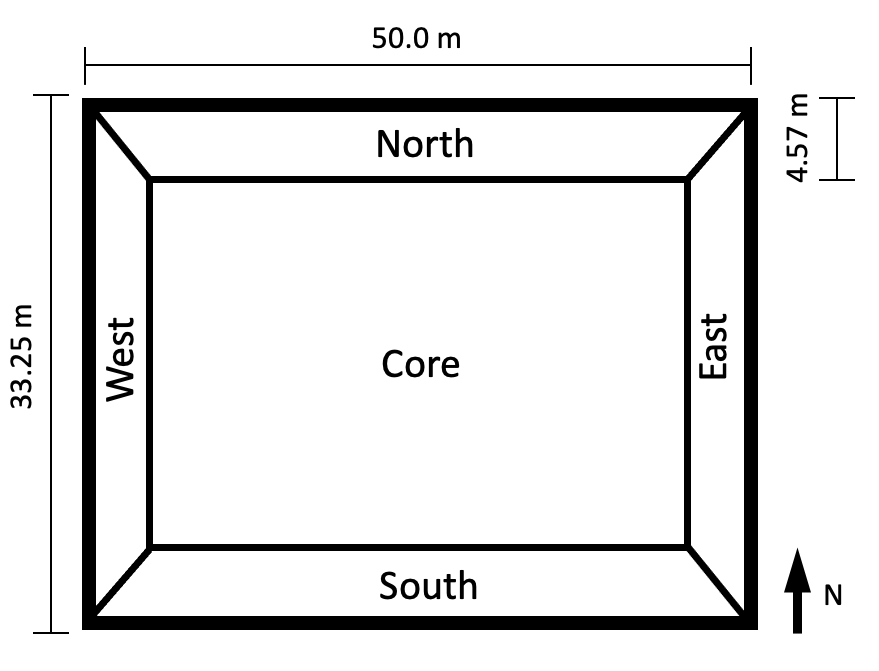
Figure 2: Illustration of five zones in Case 3 [34].

The objective of this simulation study is to empirically validate the DAD-DPC framework across three distinct simulation cases. Key differences in the specifications of these cases are summarized in Table I. Differences in building types and total areas result in varying occupant numbers and schedules. In terms of HVAC systems, Cases 2 and 3, derived from the BOPTEST challenge, employ multi-input systems, whereas Case 1 features a single-input configuration. Furthermore, unlike Cases 1 and 2, Case 3 models the building with five distinct zones, making it a multi-output system.

BOPTEST offers several APIs to facilitate simulation. The forecast API predicts weather conditions, occupant presence, and internal heat gains based on the current simulated time. In this study, only weather forecasts were utilized, as occupant and heat gain forecasts are less commonly available in real-world applications. Additionally, the results API retrieves I/O measurements, while the KPI API calculates cumulative HVAC energy costs.

IV-B Setup of controllers

The same type of comfort constraint, $\mathcal{Y}_{t}$, is applied across all three cases and is defined as follows:

$$\mathcal{Y}_{t}=\begin{cases}\{y|y\geq{21}\mathbf{I}_{n_{y}}{{}^{\circ}}C\},&\text{during occupied periods}\\ \{y|y\geq{18}\mathbf{I}_{n_{y}}{{}^{\circ}}C\},&\text{otherwise}\end{cases}$$ (12)

where the occupancy schedules for each case were detailed in the previous section. In the following, we detail the controller settings used for building climate control in the simulation.

IV-B1 Default controller

The default controllers provided by the three BOPTEST cases are described below. These controllers serve as baselines for comparison with the proposed DAD-DPC controllers.

Case 1: A local PI controller regulates the HP’s modulating signal based on feedback from the indoor temperature sensor. The evaporator fan and the floor heating system pump are activated only when the HP is on. The default controller sets the temperature to $21.2^{\circ}C$ when occupied and $20.5^{\circ}C$ when unoccupied. These setpoints are chosen to reduce discomfort caused by oscillations around the target temperature.

Case 2: This case employs three PI controllers. The first controller maintains indoor CO2 concentration below $950$ ppm by adjusting the AHU supply fan speed. The second controller regulates the AHU supply air temperature to $21^{\circ}C$ by controlling the AHU valve position. The third controller controls the indoor temperature by adjusting the radiator valve position. The default indoor temperature setpoint is $18^{\circ}C$ during unoccupied periods. Two hours before occupancy (four hours on Mondays), the setpoint is raised to $22^{\circ}C$ to reduce comfort violations.

Case 3: This case uses three PI controllers with configurations and setpoints similar to those in Case 2.

IV-B2 Setup of DAD-DPC

In this work, DAD-DPC was implemented for temperature control, while the ventilation systems continued to operate using the default controller. The I/O configurations for DAD-DPC across the three cases are summarized in Table II.

TABLE II: Summary of I/O for the DAD-DPC of three Cases

Variable	Cases
y	Case 1, 2: indoor temperature of one zone Case 3: indoor temperature of five zones
u	Case 1: HP electrical power Case 2, 3: AHU heating power, radiator heating power
w	Case 1, 2, 3: outdoor temperature, radiation

For the output $y$, Case 3 includes five dimensions corresponding to the five zones. The external input $w$ comprises the ambient dry-bulb temperature at ground level and global horizontal irradiation, as provided by the BOPTEST forecast and results APIs. For the control input $u$, heating power was selected for Cases 2 and 3, as the building thermodynamics can be reasonably approximated using linear models, making them suitable for RB-DPC. In Case 1, although nonlinearity arises from the HP’s coefficient of performance, RB-DPC effectively approximates short-term behaviors and benefits from adaptive updates for long-term operations [27].

Notably, the chosen inputs are not directly mapped to the control variables in the BOPTEST cases. For each optimal input computed by DAD-DPC, low-level controllers were employed to translate it into BOPTEST-compatible variables. In Case 1, the HP was toggled on and off within each sampling period, with on/off durations adjusted to match the desired average electrical consumption. Similarly, in Cases 2 and 3, HVAC systems were controlled by modulating setpoints or valve positions to achieve the required heating power.

Across all three cases, the following common parameters were used for DAD-DPC: sampling time, 15 minutes; prediction horizon $N$, 96 steps; initial steps $t_{init}$, 12 steps; regularization weight $Q_{g}$, 0.01$I$; regularization weight $Q_{\delta}$, 10; Hankel matrix data length $T$, 672 steps (one week); SCP data length $T_{c}$, 672 steps (one week); $\mathcal{Y}_{\text{lim}},\{y|{15}^{\circ}C\leq y\}$; $\alpha_{0}$, 0; update rate $\eta$, 0.5. The parameters, $t_{init},Q_{g},T$ were chosen based on empirical guidelines from [27]. A segmented trajectory trick from [35] was applied in DPC to reduce data requirements. Two weeks of data for $T$ and $T_{c}$ were collected using a bang-bang controller for each case. A small $\alpha_{0}$ was selected to limit frequent violations at the beginning, while a moderate update rate $\eta$ was chosen to prevent extreme adaptive adjustments. Apart from those choices, in the RB-DPC, the control objective was set to $I(y_{t},u_{t})=u_{t}$, with input constraints $\mathcal{U}$ defined as the most recent electrical or heating power levels when the respective HVAC system was on. In this simulation study, various $\alpha$ values were tested to validate the satisfaction of the violation bound (2) using DAD-DPC. The results of this validation are presented in Section IV-C.

IV-C Results of simulation cases

To validate the ability of DAD-DPC to satisfy the average comfort violation constraint (2), we evaluated its performance over two-week operation periods (1344 steps) and observed its asymptotic behavior. These two-week periods correspond to peak heating days, centered around the day with the highest 15-minute heating load of the year for each case, as determined by the BOPTEST API. The selected dates were: Case 1, January $17^{\text{th}}$ to January $30^{\text{th}}$; Case 2, February $7^{\text{th}}$ to February $20^{\text{th}}$; Case 3, December $15^{\text{th}}$ to December $28^{\text{th}}$. To reflect sensor noise, Gaussian noise $\mathcal{N}(0,0.1)$ was added to the output measurements.

Three values of $\alpha$ ($0.0125,0.05,0.2$) were tested to assess the DAD-DPC framework. Figures 3, 4 and 5 illustrate the two-week trajectories for the three cases. The top two sub-figures display the indoor temperature, and the relative cumulative power consumption, calculated as $\frac{\sum_{i=t}^{0}u_{i}}{\sum_{i=t}^{0}u_{i}^{\text{default}}}$, where $u_{t}^{\text{default}}$ is the power consumption of the corresponding default controller.

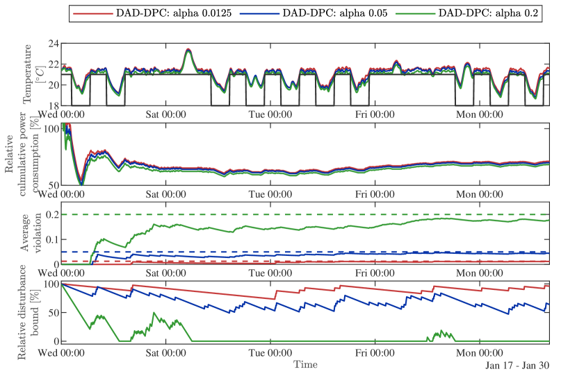
Figure 3: Case 1: indoor temperature, relative cumulative power consumption, average violations, relative disturbance bound (sub-figures from top to bottom).

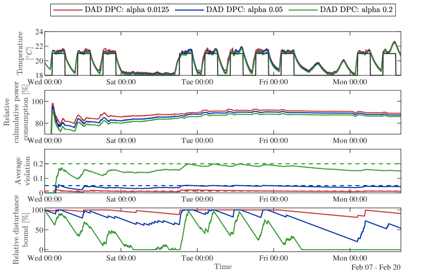
Figure 4: Case 2: indoor temperature, relative cumulative power consumption, average violations, relative disturbance bound (sub-figures from top to bottom).

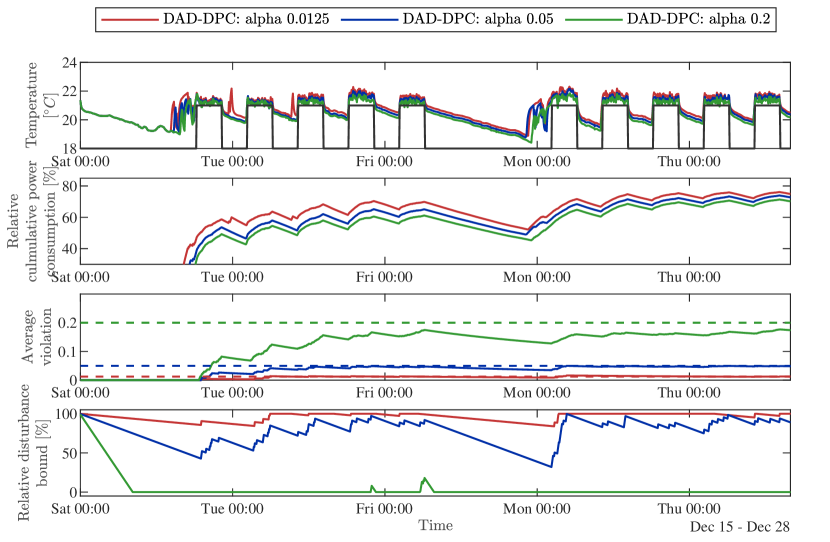
Figure 5: Case 3: indoor temperature of the west zone, relative cumulative power consumption, average violations, relative disturbance bound (sub-figures from top to bottom).

In all three cases, the indoor temperature was effectively maintained near the required comfort constraints. During unoccupied periods, the DAD-DPC relaxed the temperature to save energy. It also preheated zones before occupied periods to ensure comfort. The total power consumption across the simulations was consistently lower than that of the default controllers, demonstrating DAD-DPC’s capability to achieve energy-efficient building operation.

Moreover, the I/O trajectories exhibited consistent and reasonable behavior across the different $\alpha$ values. Larger $\alpha$ values permitted more comfort violations, leading to indoor temperatures closer to the constraint boundaries and lower power consumption. At the start of the simulations, the small initial value $\alpha_{0}=0$ induced conservative behavior, which temporarily resulted in higher cumulative power consumption compared to the default controllers (e.g., Case 1 in Figure 3). However, as $\alpha_{t}$ was adapted, this conservative behavior diminished.

The bottom two subfigures in Figures 3, 4 and 5 illustrate the average violations ($\frac{\sum_{i=0}^{t}v_{i}}{t}$), and the relative disturbance bound ($100\%*(1-\bar{\alpha}_{t})$).

With DAD-DPC, the average violation asymptotically remained within the specified level $\alpha$ across all three cases. This was achieved through adaptive disturbance updates, as shown in the bottom sub-figures. When the violation frequency was below the target $\alpha$, the relative disturbance bound decreased, encouraging more frequent violations due to Property 1, and vice versa. Across some $\alpha$ scenarios, (e.g. Case 1, $\alpha=0.05,0.2$), $\pi(x_{t},\mathcal{D}(0))$ was not activated except for the initial $\alpha_{0}$. Among these scenarios, Property 1 itself ensured a lower bound on $\alpha_{min,t}$, thereby satisfying (2). This result also confirmed that while Properties 2 and 3 are sufficient conditions, they are not strictly necessary. Additionally, based on Lemma 2, the strict violation bound (6) was occasionally satisfied due to the conservative initial setting of $\alpha_{0}=0$ was chosen (e.g., Case 1, $\alpha=0.05,0.2$). When $\alpha$ is small (e.g. $\alpha=0.0125$, Case 1, 2 and 3), $\pi(x_{t},\mathcal{D}(0))$ was applied occasionally and reduced the average violations based on Property 3.

Moreover, the average violation in most cases converged to the target bound $\alpha$. This behavior is consistent with the asymptotic lower bound (7) provided by Lemma 2. Intuitively, this lower bound ensures that when $\alpha_{t}\leq 0$, the DAD-DPC control policy leads to average violations greater than $\alpha$. The non-convergent violation behavior, observed in Case 2, $\alpha=0.2$ (Figure 4) can be explained by this mechanism. During the final days of the simulation, warmer temperatures reduced the heating demand, and even the nominal control policy, $\pi(x_{t},\mathcal{D}(1))$, failed to induce sufficient violations to meet the target. In such scenarios, choosing a smaller $Q_{\delta}$ could be a practical adjustment to increase violations.

To evaluate the trade-off between target violation levels and energy consumption, we tested the DAD-DPC with more $\alpha$ values and compared its performance with the default controller and the nominal DPC ($\pi(x_{t},\mathcal{D}(1))$). The results are presented in Figures 6, 7 and 8. For each controller, except the default, simulations were run with five Monte Carlo scenarios incorporating measurement noise. In scenarios with $\alpha=0$ across all three cases, the RB-DPC $\pi(x_{t},\mathcal{D}(0))$ resulted in minor violation levels, indicating that Property 3 held for relatively large $\alpha$ values. Theorem 3 guarantees that this property, as part of the sufficient conditions, ensures satisfaction of the asymptotic bound (2). These findings were consistent with the results of the other scenarios ($\alpha\geq 0.0125$).

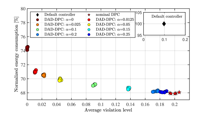
Figure 6: Case 1 during peak heating days: the normalized energy consumption and average comfort violations of different controllers.

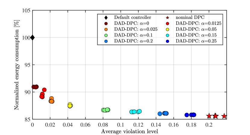
Figure 7: Case 2 during peak heating days: the normalized energy consumption and average comfort violations of different controllers.

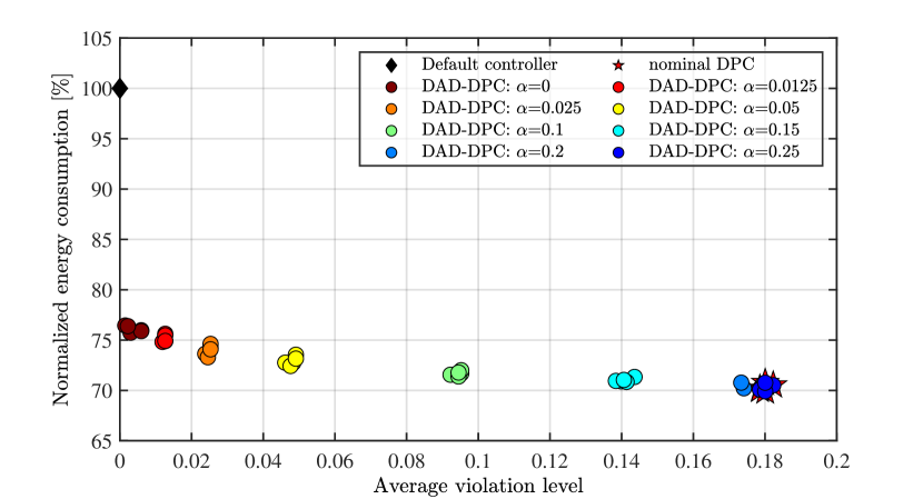
Figure 8: Case 3 during peak heating days: the normalized energy consumption and average comfort violations of different controllers.

TABLE III: Energy Consumption and Violation for Different $\alpha$ Values in Case 1, 2, 3.

Case	Type	$\alpha$ = 0	$\alpha$ = 0.0125	$\alpha$ = 0.025	$\alpha$ = 0.05	$\alpha$ = 0.10	$\alpha$ = 0.15	$\alpha$ = 0.20	$\alpha$ = 0.25	Nominal DPC
1	Energy	74.3621	71.0118	70.5104	69.8654	69.1464	68.6227	68.2155	68.1258	67.9471
	Violation	0.0001	0.0110	0.0223	0.0446	0.0912	0.1376	0.1743	0.1851	0.1993
2	Energy	90.9369	89.5555	88.4047	87.4975	86.6972	86.3736	86.0698	85.8044	85.5835
	Violation	0.0037	0.0115	0.0214	0.0426	0.0832	0.1165	0.1494	0.1805	0.2079
3	Energy	76.0857	75.1475	73.9787	72.9255	71.6832	71.0164	70.3038	70.2915	70.2915
	Violation	0.0037	0.0125	0.0249	0.0481	0.0943	0.1408	0.1774	0.1799	0.1799

The above results clearly demonstrate that lower $\alpha$ values lead to reduced average violations and increased energy consumption. The average energy consumption and violation levels across the noise scenarios are summarized in Table III. Compared to the nominal DPC, if a 5% average violation level is allowed, consistent with the European standard EN15251 Annex G [21], DAD-DPC achieves this with only a 2.82%/2.24%/3.75% increase in energy consumption while reducing violations by 77.62%/79.51%/73.26% fewer violations for Cases 1, 2 and 3, respectively.

Overall, this simulation study validates DAD-DPC’s ability to satisfy the violation bound (2) for specified $\alpha$ levels using DAD-DPC. It underscores the potential of DAD-DPC to balance average comfort violations and energy cost savings in building climate control applications.

V Case studies: experiments

This section presents experimental studies conducted to validate the efficacy of the proposed DAD-DPC framework.

V-A Setup of a real building testbed

The experiments were conducted in a real building testbed, called Polydome (Figure 9). The Polydome is a standalone building of 600 $m^{2}$, functioning as a lecture hall, exam venue and conference room with a seating capacity of 200 people. The system layout for this case study is depicted in Figure 10, where blue arrows represent the flow of cooled or heated air, and black arrows indicate the direction of data communication. The main components are detailed below.

HP: An AERMEC RTY-04 HP is installed in the Polydome. The HP operates in either heating or cooling mode. Its ventilation fan distributes ambient, cooled, or heated air throughout the building via two elongated fabric ducts, as shown by the blue arrows in Figure 10. The nominal capacities of the ventilation fan, cooling-mode compressor, and heating-mode compressor are $2.4\,kW$, $4.6\,kW$ and $6\,kW$ respectively.

Computer: A central computer (iMac with 32 GB 1600 MHz DDR3 memory and a 3.4 GHz Intel Core i7) manages several components. (1) Database: Data, including HP power consumption, indoor temperature, and historical weather data, are stored in a time-series database, InfluxDB 1.3.7 [36]. (2) DAD-DPC: The DAD-DPC framework was implemented in MATLAB. It calculated the control variables and communicated them to the HP using the Modbus serial communication protocol [37]. (3) Prediction Module: Weather forecasts, including outdoor air temperature and solar radiation, were obtained via the Tomorrow.io [38] API. Forecast data and current weather conditions were updated every 15 minutes.

Figure 9: Photo of the Polydome.

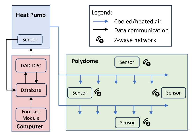
Figure 10: The overall system layout of the Polydome. Information is exchanged through wired communications and a wireless Z-wave network.

Sensors: The HP’s power consumption was monitored using an EMU 3-phase meter [39], which transmitted data to the central computer via Ethernet. Indoor temperature was monitored using four Fibaro Door/Window Sensor v2 units, installed at a height of 1.5 meters on different walls (locations shown in Figure 10). These sensors transmitted temperature data to the central computer every five minutes using the Z-wave wireless protocol. For this study, the building’s output, $y$, was calculated as the average temperature measured by the four sensors.

V-B Setup of controllers

V-B1 Default controller

The default controller implemented in the Polydome’s BMS is described here. (1) A scheduler operates the fan continuously to ensure ventilation and determines whether the HP operates in heating or cooling mode based on outdoor conditions. Access to this scheduler was not authorized for this study. (2) A bang-bang controller regulates the indoor temperature based on a setpoint and the return-air temperature, using a one ${}^{\circ}C$ deadband. For instance, in cooling mode, if the return-air temperature falls one ${}^{\circ}C$ below the setpoint, the HP activates at full power until the return-air temperature reaches the setpoint. The setpoints are fixed at ${21}^{\circ}C$ for the heating mode and ${23}^{\circ}C$ for the cooling mode.

This default controller was used as a low-level controller to execute the optimal input computed by DAD-DPC during the experiments. Additionally, data from historical days when the default controller directly operated the system are used as a baseline for comparative analysis in Section V-C.

V-B2 Setup of DAD-DPC

In the experiment, DAD-DPC was implemented for temperature control, while the HP’s ventilation and operating mode (heating or cooling) followed the default scheduler.

The I/O configuration for DAD-DPC was identical to Case 1 in the simulation study due to the similar HVAC setup, shown in Table II. Since the HP operated exclusively in either heating or cooling mode, separate I/O datasets were collected for each mode to develop the corresponding RB-DPC and SCP estimators. After the DAD-DPC computed the optimal HP electrical power, modulation similar to Case 1 was used to control the HP. By adjusting the setpoint in the default controller, the HP alternated between on and off states. The on/off durations were calculated to approximate the required electrical consumption from DAD-DPC on average.

The parameters for the DAD-DPC method were chosen as follows: sampling time, 15 minutes; prediction horizon $N$, 24 steps; initial steps $t_{init}$, 12 steps; regularization weight $Q_{g}$, 0.01$I$; regularization weight $Q_{\delta}$, 10; $\mathcal{Y}_{\text{lim}},\{y|{15}^{\circ}C\leq y\leq{30}^{\circ}C\}$. The segmented trajectory trick from [35] was employed to reduce the data requirement for Hankel matrices. In the RB-DPC, the objective was defined as $I(y_{t},u_{t})=u_{t}$ and the input constraint $\mathcal{U}$ was set to the latest maximal electrical power.

The experimental study spanned over two months and included various operational settings. The comfort constraints and parameters ($\alpha,\alpha_{0}$, $\eta$) were adjusted as described in Section IV-C. To address the nonlinearity in the HP’s coefficient of performance, adaptive updates were incorporated into the RB-DPC [27], and residual updates were applied to SCP for long-term operations. Initially, both the Hankel matrix and SCP data lengths were set to 480 steps (5 days). The required 10-day datasets for each mode were collected using the default controller.

V-C Results of experiments

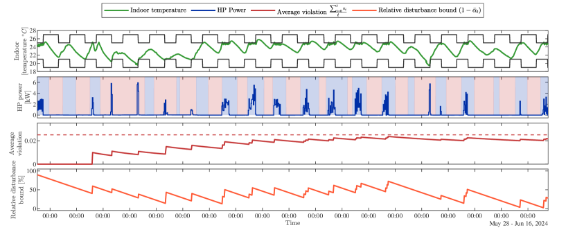
Figure 11: Scenario 1 from May 28${}^{\text{th}}$ to June 16${}^{\text{th}}$, $\alpha=0.025$. Sub-figures from top to bottom include: indoor temperature; HP’s electrical power (blue means cooling mode and red means heating mode in the background); average violations (the dashed line indicates the $\alpha$ bound); relative disturbance bound.

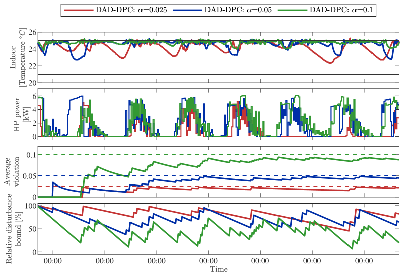
Figure 12: Three scenarios: Scenario 1 from August 20${}^{\text{th}}$ to 27${}^{\text{th}}$, $\alpha=0.025$; Scenario 2, from July 30${}^{\text{th}}$ to August 6${}^{\text{th}}$, $\alpha=0.05$; Scenario 3 from August 6${}^{\text{th}}$ to 13${}^{\text{rd}}$, $\alpha=0.025$; Sub-figures from top to bottom include: indoor temperature; HP’s electrical power (always in cooling mode); average violations (the dashed lines indicate three $\alpha$ bounds); relative disturbance bound.

This section presents the results from four DAD-DPC operational scenarios spanning a total of 40 days, designed to validate the framework’s efficacy. Additional scenarios, covering 37 days, are included in Appendix -A as they provide less critical insights.

• Scenario 1. Duration: 19 days from May 28${}^{\text{th}}$ to June 16${}^{\text{th}}$, 2024; Parameters: $21^{\circ}C\leq y_{t}\leq 25^{\circ}C$ from 8 a.m. to 6 p.m., $19^{\circ}C\leq y_{t}\leq 27^{\circ}C$ otherwise, $\alpha=0.025$, $\alpha_{0}=0.1$, $\eta=0.1$.

• Scenario 2. Duration: 7 days from August 20${}^{\text{th}}$ to 27${}^{\text{th}}$, 2024; Parameters: $21^{\circ}C\leq y_{t}\leq 25^{\circ}C$ at any time, $\alpha=0.025$, $\alpha_{0}=0$, $\eta=0.1$.

• Scenario 3. Duration: 7 days from July 30${}^{\text{th}}$ to August 6${}^{\text{th}}$, 2024; Parameters: $\alpha=0.05$, others are the same as Scenario 2.

• Scenario 4. Duration: 7 days from August 6${}^{\text{th}}$ to 13${}^{\text{rd}}$, 2024; Parameters: $\alpha=0.1$, others are the same as Scenario 2.

Figure 11 presents the results for Scenario 1, which corresponds to the transitional period between spring and summer. During this time, the HP frequently alternated between heating and cooling modes due to varying outdoor temperatures.

The first two sub-figures in Figure 11 depict the indoor temperature dynamics and the HP’s power consumption. The DAD-DPC effectively maintained the indoor temperature within the specified comfort constraints for most of the period, even with frequent mode switching between heating and cooling. The third and fourth sub-figures depict the average violation levels and the adaptive disturbance bound updates. The average violation level converged to the specified $\alpha=0.025$, demonstrating the effectiveness of the DAD-DPC framework. This result was achieved because the well-designed DAD-DPC dynamically adjusted the disturbance bound in response to violations, ensuring that $\alpha_{t}$ remained bounded. As observed in the asymptotic behavior of the around 1800-step operation, both the upper bound (2) and lower bound (7) were satisfied, consistent with the guarantees by Lemma 2. Additionally, with a small $\alpha_{0}=0$, the strict bound (6) was also satisfied.

Scenarios 2, 3 and 4 were conducted during the summer to evaluate the performance of DAD-DPC under different violation bounds, i.e. $\alpha\in\{0.025,0.05,0.1\}$. All the other parameters were the same, and constant comfort constraints were applied to ensure a fair comparison with the default controller. The closed-loop trajectories for these scenarios are shown in Figure 12, with distinct colors representing different settings. Since these scenarios occurred during the summer in Lausanne, the HP primarily operated in cooling mode, and the indoor temperature often approached the upper comfort bound. Direct comparison of input and output behaviors across different $\alpha$ values is challenging due to varying weather conditions. For instance, in Scenario 2, cooler weather occasionally caused the indoor temperature to drop to 22^∘. In the fourth sub-figure, the relative disturbance bound is shown to adaptively update, with smaller $\alpha$ values resulting in larger bounds to ensure fewer violations. Consequently, the average violations in each scenario converged to their respective chosen bounds, satisfying the violation constraint (2), as seen in the third sub-figure.

To compare the violations and energy consumption under different $\alpha$settings, continuous days with similar weather conditions were selected: Scenario 3 (from July 31${}^{\text{st}}$ to August 5${}^{\text{th}}$), Scenario 4 (from August 6${}^{\text{th}}$ to 10${}^{\text{th}}$), and the default controller (from August 29${}^{\text{th}}$ to September 1${}^{\text{st}}$). The statistical results are summarized in Table IV. Scenario 2 was excluded from this comparison due to cooler weather. Scenarios 3 and 4 demonstrated substantial energy savings, reducing consumption by 20.54% and 24.39% , respectively, compared to the default controller. Furthermore, Scenario 3 increased energy consumption by only 5.09% compared to Scenario 4 while achieving 39.76% fewer comfort violations. This result empirically demonstrates the trade-off between comfort violations and energy savings enabled by DAD-DPC.

TABLE IV: Comparison of scenarios with different controllers under similar weather conditions.

	Average Violation	Average Hourly Energy Consumption $[kWh]$	Average Outdoor Temperature $[^{\circ}C]$	Average Solar Radiation $[kW/m^{2}]$
Scenario 3	0.050	1.671	23.108	0.257
Scenario 4	0.083	1.590	23.087	0.253
Default	0.000	2.103	23.089	0.219

VI Conclusion

This paper proposes a DAD-DPC framework designed to ensure the asymptotic average violation bound. As a practical application in building climate control, we developed a fully data-driven implementation of DAD-DPC utilizing Willems’ Fundamental Lemma and conformal prediction. The framework’s performance was evaluated through simulations on the high-fidelity BOPTEST platform and experiments on the Polydome testbed. With a 5% violation bound, the DAD-DPC framework achieved reductions in comfort violations of 77.62%/79.51%/73.26%/39.76% while increasing energy consumption by only 2.82%/2.24%/3.75%/5.09% (three simulation cases and one experimental case) compared to other controller configurations. These results underscore the framework’s capability to balance energy efficiency and comfort effectively, showcasing its potential for practical deployment in building climate control systems.

-A Other experiment results

This appendix describes additional experimental scenarios conducted in the Polydome testbed, spanning a total of 36 days.

• Scenario 5. Duration: 7 days from August 13${}^{\text{th}}$ to 20${}^{\text{th}}$, 2024; Parameters: $21^{\circ}C\leq y_{t}\leq 25^{\circ}C$ at any time, $\alpha=0.05$, $\alpha_{0}=1$, $\eta=0.1$.

• Scenario 6. Duration: 14 days from May 14${}^{\text{th}}$ to 28${}^{\text{th}}$, 2024; Parameters: $21^{\circ}C\leq y_{t}\leq 25^{\circ}C$ from 8 a.m. to 6 p.m., $19^{\circ}C\leq y_{t}\leq 27^{\circ}C$ otherwise, $\alpha=0.05$, $\alpha_{0}=0.1$, $\eta=0.03$.

• Scenario 7. Duration: 8 days from July 7${}^{\text{th}}$ to 15${}^{\text{th}}$, 2024; Parameters: $21^{\circ}C\leq y_{t}\leq 25^{\circ}C$ from 8 a.m. to 6 p.m., $19^{\circ}C\leq y_{t}\leq 27^{\circ}C$ otherwise, $\alpha=0.025$, $\alpha_{0}=0.1$, $\eta=0.1$.

• Scenario 8. Duration: 7 days from July 17${}^{\text{th}}$ to 24${}^{\text{th}}$, 2024; Parameters: $21^{\circ}C\leq y_{t}\leq 25^{\circ}C$ from 8 a.m. to 6 p.m., $19^{\circ}C\leq y_{t}\leq 27^{\circ}C$ otherwise, $\alpha=0.025$, $\alpha_{0}=0$, $\eta=0.1$.

Scenario 5 used the same parameter as Scenario 3 in Section V-C, except for a larger initial $\alpha_{0}=1$. As shown in Figure 13, the average violation ultimately converged to satisfy the asymptotic bound (2). However, during the operation, the average violation was higher than $\alpha$, consistent with the behavior indicated by (5) due to the large $\alpha_{0}$.

As shown in Figure 13, Scenario 6 occurred during a mild transition period, similar to Scenario 1 in Section V-C. Due to the relatively high violation bound $\alpha=0.05$, the system eventually operated as a nominal DPC $\pi(x_{t},\mathcal{D}(1))$. The adaptive updates progressed slowly because of the small update factor $\eta=0.03$, which also affected the convergence speed, as indicated by (5)

Scenarios 7 and 8, which shared similar parameters, are illustrated in Figures 15 and 16. However, Scenario 7 utilized two compressors in the HP, which allowed for increased input power and a larger input constraint. Consequently, the indoor temperature in Scenario 7 remained closer to the upper comfort bound, reflecting less conservative control compared to Scenario 8.

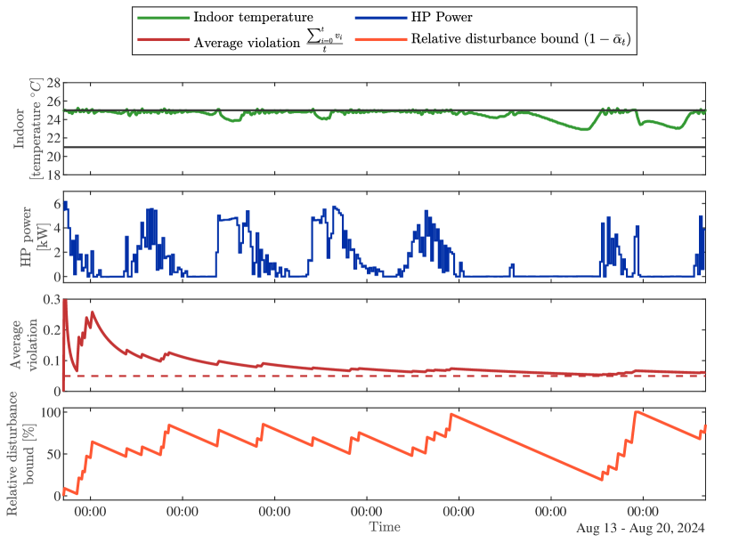
Figure 13: Scenario 5 from August 13${}^{\text{th}}$ to 20${}^{\text{th}}$, $\alpha=0.05$. Sub-figures from top to bottom include: indoor temperature; HP’s electrical power (always in cooling mode); average violations (the dashed line indicates the $\alpha$ bound); relative disturbance bound.

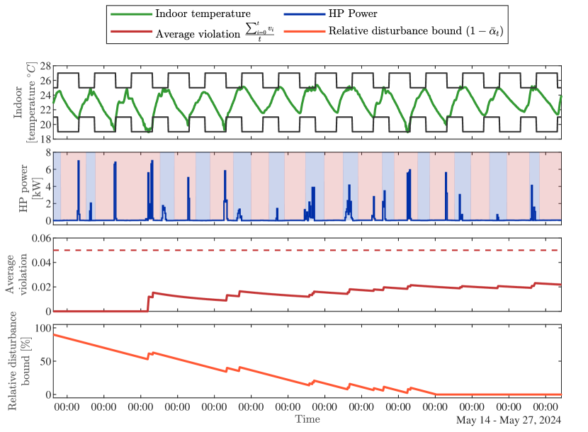
Figure 14: Scenario 6 from May 14${}^{\text{th}}$ to 28${}^{\text{th}}$, $\alpha=0.05$. Sub-figures from top to bottom include: indoor temperature; HP’s electrical power (blue means cooling mode and red means heating mode in the background); average violations (the dashed line indicates the $\alpha$ bound); relative disturbance bound.

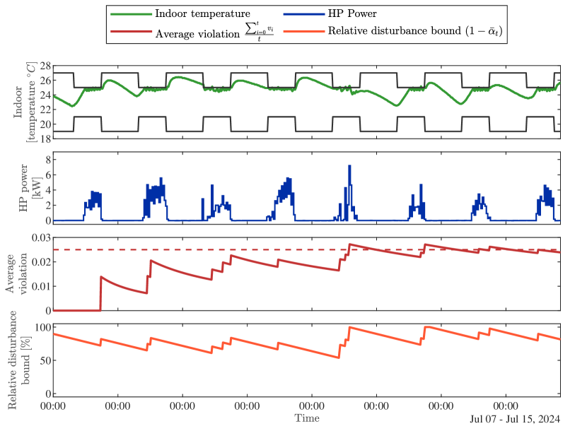
Figure 15: Scenario 7 from July 7${}^{\text{th}}$ to 15${}^{\text{th}}$, $\alpha=0.025$. Sub-figures from top to bottom include: indoor temperature; HP’s electrical power (always in cooling mode); average violations (the dashed line indicates the $\alpha$ bound); relative disturbance bound.

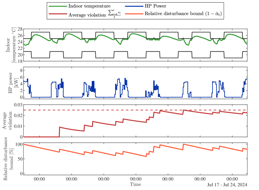
Figure 16: Scenario 8 from July 17${}^{\text{th}}$ to 24${}^{\text{th}}$, $\alpha=0.025$. Sub-figures from top to bottom include: indoor temperature; HP’s electrical power (always in cooling mode); average violations (the dashed line indicates the $\alpha$ bound); relative disturbance bound.

References

- [1] U. N. E. Programme, “2023 global status report for buildings and construction,” 2023.
- [2] T. I. Salsbury, “A survey of control technologies in the building automation industry,” IFAC Proceedings Volumes, vol. 38, no. 1, pp. 90–100, 2005.
- [3] J. Drgoňa, J. Arroyo, I. C. Figueroa, D. Blum, K. Arendt, D. Kim, E. P. Ollé, J. Oravec, M. Wetter, D. L. Vrabie, et al., “All you need to know about model predictive control for buildings,” Annual Reviews in Control, vol. 50, pp. 190–232, 2020.
- [4] M. Killian and M. Kozek, “Ten questions concerning model predictive control for energy efficient buildings,” Building and Environment, vol. 105, pp. 403–412, 2016.
- [5] Y. Balali, A. Chong, A. Busch, and S. O’Keefe, “Energy modelling and control of building heating and cooling systems with data-driven and hybrid models—a review,” Renewable and Sustainable Energy Reviews, vol. 183, p. 113496, 2023.
- [6] P. Stoffel, L. Maier, A. Kümpel, T. Schreiber, and D. Müller, “Evaluation of advanced control strategies for building energy systems,” Energy and Buildings, vol. 280, p. 112709, 2023.
- [7] E. N. Pergantis, N. Al Theeb, P. Dhillon, J. P. Ore, D. Ziviani, E. A. Groll, K. J. Kircher, et al., “Field demonstration of predictive heating control for an all-electric house in a cold climate,” Applied Energy, vol. 360, p. 122820, 2024.
- [8] T. Xiao and F. You, “Building thermal modeling and model predictive control with physically consistent deep learning for decarbonization and energy optimization,” Applied Energy, vol. 342, p. 121165, 2023.
- [9] F. Bünning, B. Huber, A. Schalbetter, A. Aboudonia, M. H. de Badyn, P. Heer, R. S. Smith, and J. Lygeros, “Physics-informed linear regression is competitive with two machine learning methods in residential building mpc,” Applied Energy, vol. 310, p. 118491, 2022.
- [10] F. Jorissen, W. Boydens, and L. Helsen, “Taco, an automated toolchain for model predictive control of building systems: implementation and verification,” Journal of building performance simulation, vol. 12, no. 2, pp. 180–192, 2019.
- [11] Y. Lian, J. Shi, M. Koch, and C. N. Jones, “Adaptive robust data-driven building control via bilevel reformulation: An experimental result,” IEEE Transactions on Control Systems Technology, vol. 31, no. 6, pp. 2420–2436, 2023.
- [12] L. Di Natale, Y. Lian, E. T. Maddalena, J. Shi, and C. N. Jones, “Lessons learned from data-driven building control experiments: Contrasting gaussian process-based mpc, bilevel deepc, and deep reinforcement learning,” in 2022 IEEE 61st conference on decision and control (CDC), pp. 1111–1117, IEEE, 2022.
- [13] A. Bemporad and M. Morari, “Robust model predictive control: A survey,” in Robustness in identification and control, pp. 207–226, Springer, 2007.
- [14] A. Mesbah, “Stochastic model predictive control: An overview and perspectives for future research,” IEEE Control Systems Magazine, vol. 36, no. 6, pp. 30–44, 2016.
- [15] F. Oldewurtel, A. Parisio, C. N. Jones, D. Gyalistras, M. Gwerder, V. Stauch, B. Lehmann, and M. Morari, “Use of model predictive control and weather forecasts for energy efficient building climate control,” Energy and buildings, vol. 45, pp. 15–27, 2012.
- [16] M. Korda, R. Gondhalekar, F. Oldewurtel, and C. N. Jones, “Stochastic model predictive control: Controlling the average number of constraint violations,” in 2012 IEEE 51st IEEE Conference on Decision and Control (CDC), pp. 4529–4536, IEEE, 2012.
- [17] F. Oldewurtel, D. Sturzenegger, P. M. Esfahani, G. Andersson, M. Morari, and J. Lygeros, “Adaptively constrained stochastic model predictive control for closed-loop constraint satisfaction,” in 2013 American Control Conference, pp. 4674–4681, IEEE, 2013.
- [18] M. Korda, R. Gondhalekar, F. Oldewurtel, and C. N. Jones, “Stochastic mpc framework for controlling the average constraint violation,” IEEE Transactions on Automatic Control, vol. 59, no. 7, pp. 1706–1721, 2014.
- [19] J. Fleming and M. Cannon, “Time-average constraints in stochastic model predictive control,” in 2017 American Control Conference (ACC), pp. 5648–5653, IEEE, 2017.
- [20] J. Shi and C. N. Jones, “Disturbance-adaptive model predictive control for bounded average constraint violations using conformal prediction,” 2024.
- [21] C. Comite’Europe’en de Normalisation, “Indoor environmental input parameters for design and assessment of energy performance of buildings addressing indoor air quality, thermal environment, lighting and acoustics,” EN 15251, 2007.
- [22] M. Sourbron and L. Helsen, “Evaluation of adaptive thermal comfort models in moderate climates and their impact on energy use in office buildings,” Energy and Buildings, vol. 43, no. 2-3, pp. 423–432, 2011.
- [23] J. C. Willems, P. Rapisarda, I. Markovsky, and B. L. De Moor, “A note on persistency of excitation,” Systems & Control Letters, vol. 54, no. 4, pp. 325–329, 2005.
- [24] F. Dorfler, J. Coulson, and I. Markovsky, “Bridging direct & indirect data-driven control formulations via regularizations and relaxations,” IEEE Trans on Autom Control, 2022.
- [25] M. Yin, H. Cai, A. Gattiglio, F. Khayatian, R. S. Smith, and P. Heer, “Data-driven predictive control for demand side management: Theoretical and experimental results,” Appl Energy, vol. 353, p. 122101, 2024.
- [26] V. Chinde, Y. Lin, and M. J. Ellis, “Data-enabled predictive control for building hvac systems,” J of Dyn Syst, Meas, and Control, vol. 144, no. 8, p. 081001, 2022.
- [27] J. Shi, Y. Lian, C. Salzmann, and C. N. Jones, “Adaptive data-driven predictive control as a module in building control hierarchy: A case study of demand response in switzerland,” arXiv preprint arXiv:2307.08866, 2023.
- [28] J. Berberich, J. Köhler, M. A. Müller, and F. Allgöwer, “Robust constraint satisfaction in data-driven mpc,” in 2020 59th IEEE Conference on Decision and Control (CDC), pp. 1260–1267, IEEE, 2020.
- [29] J. Shi, Y. Lian, and C. N. Jones, “Efficient recursive data-enabled predictive control,” in 2024 European Control Conference (ECC), IEEE, 2024.
- [30] V. Vovk, A. Gammerman, and G. Shafer, Algorithmic learning in a random world, vol. 29. Springer, 2005.
- [31] A. N. Angelopoulos and S. Bates, “A gentle introduction to conformal prediction and distribution-free uncertainty quantification,” arXiv preprint arXiv:2107.07511, 2021.
- [32] D. Blum, J. Arroyo, S. Huang, J. Drgoňa, F. Jorissen, H. T. Walnum, Y. Chen, K. Benne, D. Vrabie, M. Wetter, et al., “Building optimization testing framework (boptest) for simulation-based benchmarking of control strategies in buildings,” Journal of Building Performance Simulation, vol. 14, no. 5, pp. 586–610, 2021.
- [33] “Adrenalin boptest challenge: Smart building hvac control.” https://adrenalin.energy/BOPTEST-Challenge-Smart-building-HVAC-control. Accessed: 2024-12-02.
- [34] M. Deru, B. Griffith, N. Long, M. Halverson, D. Winiarski, J. Huang, and D. Crawley, “Doe commercial building research benchmarks for commercial buildings,” preparation. US DOE, 2008.
- [35] E. O’Dwyer, E. C. Kerrigan, P. Falugi, M. Zagorowska, and N. Shah, “Data-driven predictive control with improved performance using segmented trajectories,” IEEE Transactions on Control Systems Technology, vol. 31, no. 3, pp. 1355–1365, 2022.
- [36] “Influxdb.” https://www.influxdata.com. Accessed: 2022-07-01.
- [37] A. Swales et al., “Open Modbus/TCP specification,” Schneider Electric, vol. 29, pp. 3–19, 1999.
- [38] “Tomorrow.io.” https://www.tomorrow.io. Accessed: 2022-07-01.
- [39] “Emu electronics ag.” https://www.emuag.ch/. Accessed: 2022-07-01.