Point-set registration in bounded domains via the Fokker-Planck equation
Abstract
We present a point set registration method in bounded domains based on the solution to the Fokker Planck equation. Our approach leverages (i) density estimation based on Gaussian mixture models; (ii) a stabilized finite element discretization of the Fokker Planck equation; (iii) a specialized method for the integration of the particles. We review relevant properties of the Fokker Planck equation that provide the foundations for the numerical method. We discuss two strategies for the integration of the particles and we propose a regularization technique to control the distance of the particles from the boundary of the domain. We perform extensive numerical experiments for two two-dimensional model problems to illustrate the many features of the method.
1 Introduction
Point set registration (PSR) is the process of finding a spatial transformation that aligns two point clouds. Given the domain and the reference and the point clouds , we seek a transformation such that the mapped point cloud is close — in the sense of Hausdorff — to the target point cloud. For several applications, it is also important to identify a (possibly non-autonomous) flow of diffeomorphisms to coherently deform the reference point cloud into . In this note, we focus on the problem of PSR in moderate-dimensional ( or ) bounded domains; we target applications in model order reduction (MOR) where coordinate transformations are employed to align coherent features of the solution field [4, 9, 10, 21]; we also envision applications to data assimilation tasks that involve the interpolation between point clouds in complex geometries.
We propose a PSR method based on the solution to the Fokker Planck (FP) equation. First, we model the reference and the target point clouds as independent identically distributed samples from two continuous distributions with densities and , respectively. Second, we estimate and using Gaussian mixture models. Third, we solve a suitable FP equation to determine a flow of probability densities that is equal to at time , and converges to as . Fourth, we exploit the properties of the FP equation to obtain the desired morphing based on the knowledge of at all times.
The FP equation describes the evolution of a probability density under diffusion and drift: it reads as a linear parabolic equation with Neumann boundary conditions on , constant diffusion and time-independent advection. The FP equation has been extensively employed in Information Theory [7], stochastic processes in Physics and Chemistry [22], and more recently in machine learning for generative modeling [20]. The solution to the FP equation is tightly linked to the solution to optimal transportation (OT) problems [19]: however, while the FP equation is a linear parabolic equation with time-independent coefficients, the evolution equation associated to OT problems is highly nonlinear and much more difficult to handle, despite the many recent contributions to the field [15].
The outline of the note is as follows. In section 2, we introduce the FP equation and we discuss relevant properties that are exploited in the remainder of the note. In section 3, we present the numerical method: first, we introduce the discretization of the FP equation, which is based on the finite element method for space discretization and on the Crank Nicolson method for time integration; second, we discuss two distinct methods for the transport of the point clouds; third, we present a regularization approach to control the distance of the particles from the boundary; fourth, we briefly review the problem of density estimation through Gaussian mixtures. In section 4, we present several numerical results in two dimensions that illustrate the performance of the method. Section 5 concludes the paper.
2 Mathematical background
We review select properties of the Fokker Planck (FP) equation that provide the mathematical foundation for the method. We emphasize that the FP equation has been the subject of extensive studies in Analysis and Calculus of Variations; in particular, the material of this section relies heavily on [7, 11, 14, 19]. Below, is a Lipschitz domain in , while refers to the space of probability density functions (pdfs) with bounded second-order moments; the acronym “a.s.” (resp., “a.e.”) stands for “almost surely” (resp., “almost every”) with respect to the Lebesgue measure in and the acronym “i.i.d.” stands for “independent identically distributed”.
2.1 Kullback-Leibler divergence
Given the densities , we introduce the Kullback-Leibler (KL) divergence between and as [12]
| (1) |
Note that is infinite if the support of does not contain the support of . Theorem 2.1 summarizes key properties of the KL divergence.
Theorem 2.1.
The following hold.
-
1.
Given the densities , and if and only if a.s..
-
2.
The KL divergence (1) is asymmetric, that is in general .
-
3.
The KL divergence (1) is strongly convex, that is, given and , we have
where the latter holds with equality if and only if a.s..
-
4.
(Pinsker’s inequality) The KL divergence (1) satisfies .
We provide the proof of Theorem 2.1 in Appendix A. We notice that the KL divergence is minimized when (cf. Property 1); as discussed below, the strong convexity property and the Pinsker’s inequality are the key to prove the existence of paths that link the initial and the target distributions (cf. Theorem 2.2). We further remark that the KL divergence is not a distance in since it is not symmetric (cf. Property 2). If we denote by the potential associated with the density , we can express (1) as:
| (2) |
In Bayesian inference, the first term in (2) is interpreted as an entropy function, while the second term is interpreted as a potential energy and the sum of the two terms is interpreted as a free-energy function (see, e.g., [5]).
2.2 Fokker-Plank equation
Let and let ; then, we define the Fokker-Plank (FP) equation:
| (3) |
where denotes the outward normal to . We assume that is strictly positive in and is sufficiently smooth to ensure that is Lipschitz continuous. We introduce the spaces and and the weak formulation of the FP equation (3): find such that and
| (4) |
Theorem 2.2.
Let be a Lipschitz domain in ; let satisfy (i) , and (ii) is Lipschitz-continuous in . The following hold.
Theorem 2.2 provides the foundations for the use of the FP equation for point-set registration. The first statement ensures the existence and the uniqueness of the solution to (3); the second statement ensures that is a pdf for all ; the third statement shows that converges to the target distribution for ; finally, the fourth statement provides a constructive way to sample from the target distribution and also to generate trajectories that link initial and target pdfs.
2.3 Fokker-Plank equation and gradient flows
The authors of [11] showed that the FP equation can be interpreted as the gradient flow of the KL divergence with respect to the Wasserstein metric. We can hence interpret the solution to the time-discrete FP equation as the solution to a sequence of (linearized) optimal transport problems. Below, we provide an informal proof of this statement for ; we refer to [11] for the rigorous derivation and for further details.
First, we recall the 2-Wasserstein metric between the densities and :
| (6) |
It is possible to show that the optimal transport map is of the form where is the identity map and (cf. [2], see also [19, Chapter 1.3.1]). Therefore, we can restate (6) as
| (7) |
We denote by the time grid, and we denote by the estimate of at time ; we assume that results from the evaluation of subject to a potential velocity field with . We express . Since satisfies with , exploiting the Jacobi formula for the derivative of the determinant, we find
| (8) |
We seek to maximize the first variation of the KL divergence for a fixed Wasserstein distance:
| (9) |
where is a given constant and . If we integrate by part the objective of (9), we find
In conclusion, we can restate (9) as
| (10) |
The optimality conditions for (10) are
| (11) |
where . If we integrate by part the second term in the first equation of (11), we find111We here exploit the fact that the space is dense in .
where the constant is a function of that is determined by substituting the latter expression in (11)2. We conclude that for an appropriate choice of in (9) we have
which is the explicit Euler discretization of the FP equation.
2.4 Transport of Gaussian random variables
We denote by the pdf associated with an univariate Gaussian random variable with mean and variance . We assume that and . It is possible to show that the solution to the FP equation in is given by (see, e.g., [22, Chapter VIII.4])
| (12) |
For comparison, we recall the McCann interpolation between the same two Gaussian random variables, which corresponds to the geodesic (shortest path) in the Wasserstein metric (see, e.g., [15, Remark 2.31])
| (13) |
We observe that the solution to (3) connects to in infinite time at non-constant speed, while the optimal transport map achieves the same goal in finite time and at constant speed. Note, nevertheless, that the convergence of to is exponentially-fast: this observation motivates the use of adaptive time stepping strategies to integrate (14).
3 Methodology
3.1 High-fidelity discretization
We rely on the finite element (FE) method to discretize (4) in space, and on the Crank-Nicolson method for time integration. Given the time grid and the FE space , we define the sequence of approximate solutions such that and
| (14) |
for . We remark that problem (14) might feature strong advection: for this reason, in the numerical experiments, we resort to a SUPG stabilization of (14) to avoid spurious oscillations [3].
Given the particles , we consider two distinct strategies to generate the approximate trajectories: the “ODE” method and the “gradient flow (GF)” method. The former is justified by Property 4 in in Theorem 2.2, while the latter is motivated by the discussion in section 2.3.
ODE method.
In this approach, we discretize the ODE system
| (15) |
where and is a suitable approximation of the density in the interval . In the numerical experiments, we consider an explicit Euler discretization of (15) based on a single time step:
| (16) |
We also consider an explicit second-order Runge-Kutta (RK2) scheme for (15) based on the linear interpolation of the density field
To further increase accuracy, we also lower the time step used for (15).
GF method.
Given the estimates obtained through (14), we compute the potential such that
| (17a) | |||
| and then we estimate the positions of the particles as | |||
| (17b) | |||
Note that (17a) corresponds to the linearization of the Monge-Ampere equation; in future works, we shall exploit this analogy to determine higher-order approximations of the trajectories of the particles. We observe that the linear system associated with (17a) is poorly conditioned when is small. In the numerical examples, we consider the regularized problem:
| (18) |
where is a regularization parameter that is set equal to in the numerical experiments.
3.2 Treatment of boundaries
For several applications, we envision that it is necessary to control the distance of the particles from the boundaries of the domain. In our setting, this can be achieved by introducing a regularization in the potential . In more detail, we consider the regularized potential
| (19) |
where is a (regularized) distance function from the boundary of . The second term in (19) introduces a repulsive force that is active in the proximity of the boundary and prevents particles from approaching the boundary too closely. The constant is a regularization parameter whose choice is investigated in the numerical examples, while the constant is the smoothing parameter that is introduced below.
In order to define the function in (19), we first introduce the distance function , , where the user-defined tolerance tol prevents division by zero in (19). Since the distance function is in general only Lipschitz continuous, we apply a smoothing to ensure that is sufficiently smooth. We consider a non-conforming approximation of the biharmonic equation for smoothing [13]. We denote by the j-th facet of the mesh, by the positive normal to each facet, by the -th element of the mesh, by the set of internal facets of the mesh. Given the field , we define the positive and the negative limits on the facets of the mesh
then, we introduce the normal jump of the gradient at each facet and the facet average . Exploiting the previous definitions, we define the smoothing problem: find such that and
| (20a) | |||
| where | |||
| (20b) | |||
| and with , and equal to the polynomial degree of the FE basis. | |||
3.3 Estimate of the target density
The application of the FP equation to PSR requires the estimate of the densities and . Given the initial and the target point clouds and , we fit two Gaussian mixture models (GMMs) to determine the estimates of and that enter in (14) (see, e.g., [8, Chapter 8]). We resort to the Matlab function fitgmdist to determine the GMMs associated with the point clouds. We determine the number of mixture models using the Aikake information criterion (AIC); furthermore, we introduce a regularization of the covariance matrix to robustify the learning procedure222We consider the regularization value ; see the Matlab documentation for further details..
The use of GMMs for density estimation ensures that and are strictly positive for all , which is crucial to apply the results of Theorem 2.2. Furthermore, we recall that for Gaussian distributions we have
This implies that for GMMs the gradient of grows linearly with respect to the distance from the centers of the mixture models.
4 Numerical results
4.1 Transport of Gaussian distributions across a cylinder
4.1.1 Problem setting
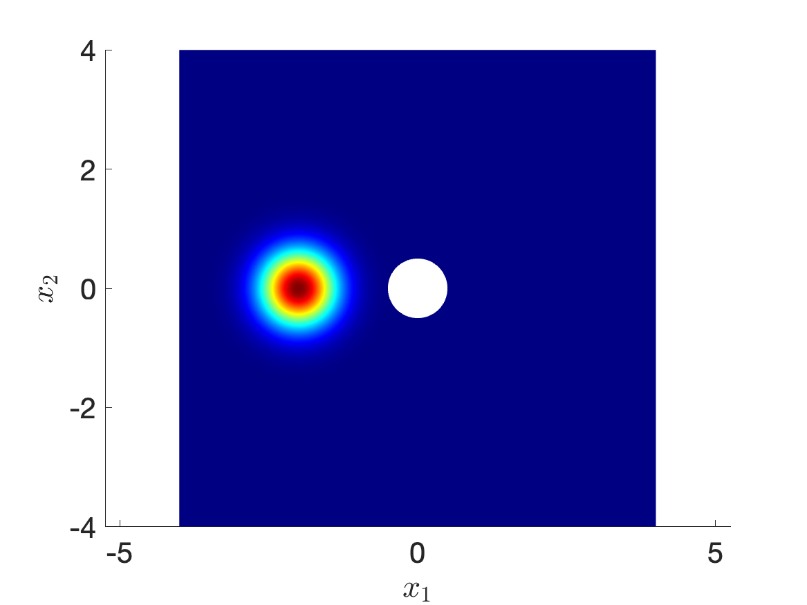
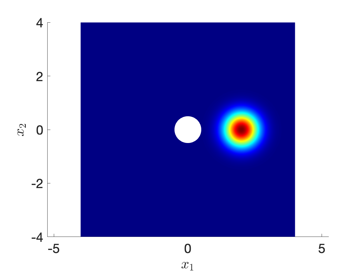
We consider the problem of transporting the Gaussian density with and to with and in the domain . Figure 1 shows the initial and the target distributions.
We resort to a P2 FE discretization with degrees of freedom; we integrate the equation in the time interval and we consider the grid
| (21) |
The non-homogeneous time discretization is motivated by the observation that the dynamics is much faster at the onset of the simulation; in the future, we plan to implement more rigorous adaptive time stepping strategies. We further remark that is computed by differentiating the FE approximation of : we notice that approximating the density through its nodal representation and then computing as leads to significantly less accurate results. The regularized distance function in (19) is computed using and and several values of .
To validate the PSR procedure, we generate with and we compare the trajectories obtained using our method with iid samples from the target distribution. Time integration of the particles is performed using the ODE method based on the explicit Euler method (16) with the same time step that is used for the integration of (14). We also considered the GF method and the ODE method with RK2 time integration: since the results of the latter two methods are nearly equivalent to the ones obtained using (16), we do not report them here.
4.1.2 Results
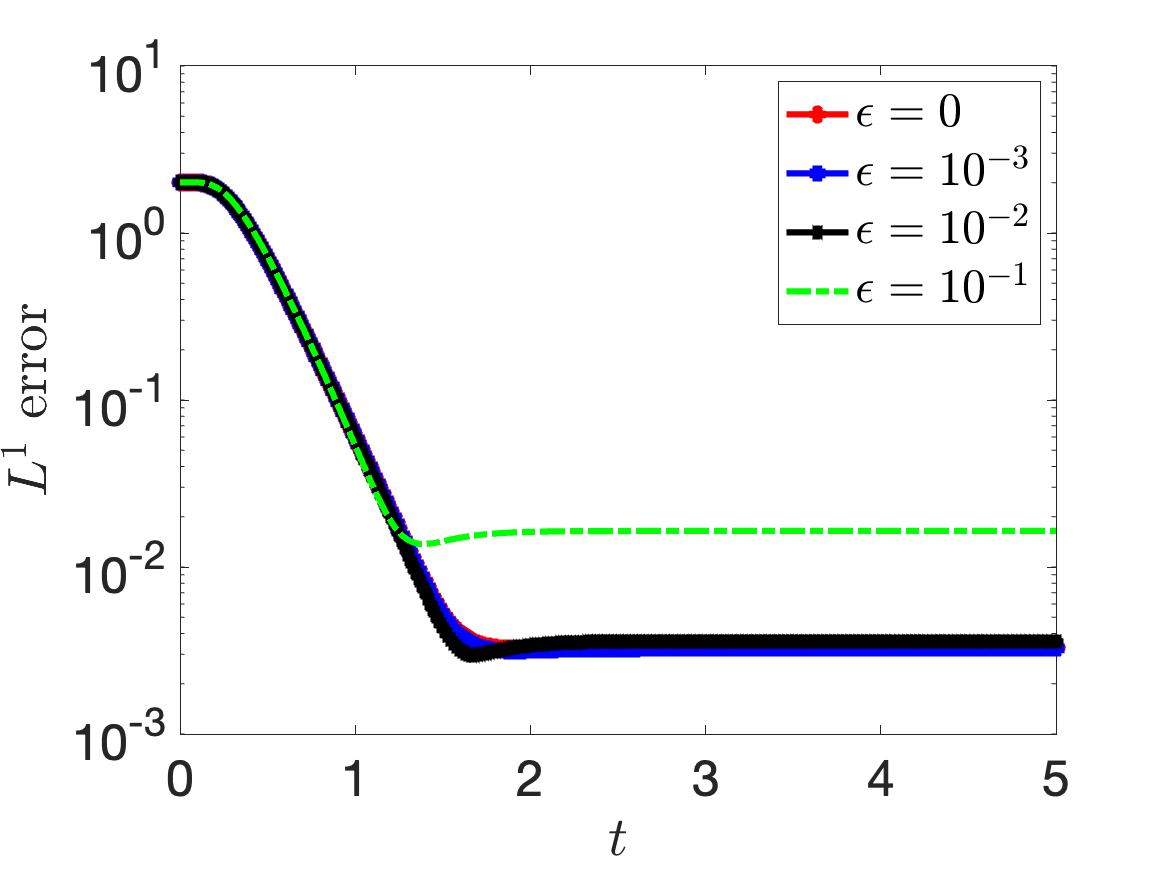
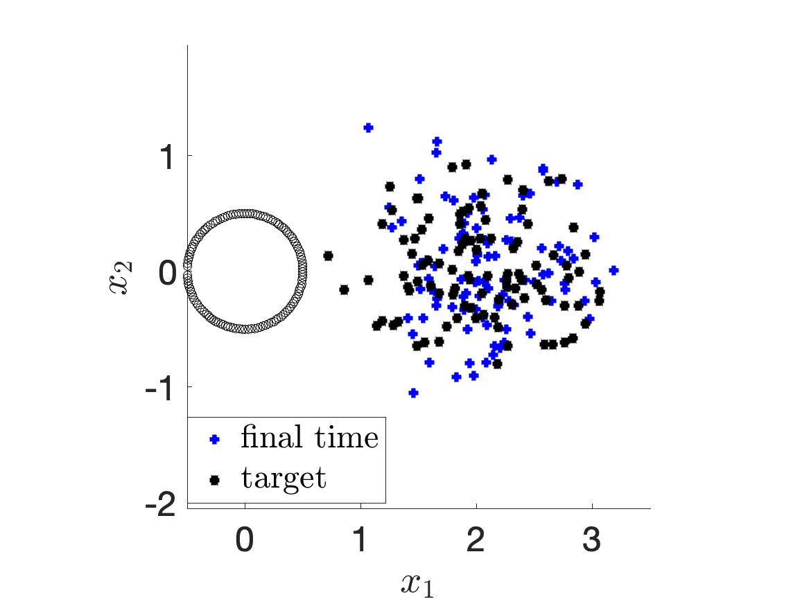
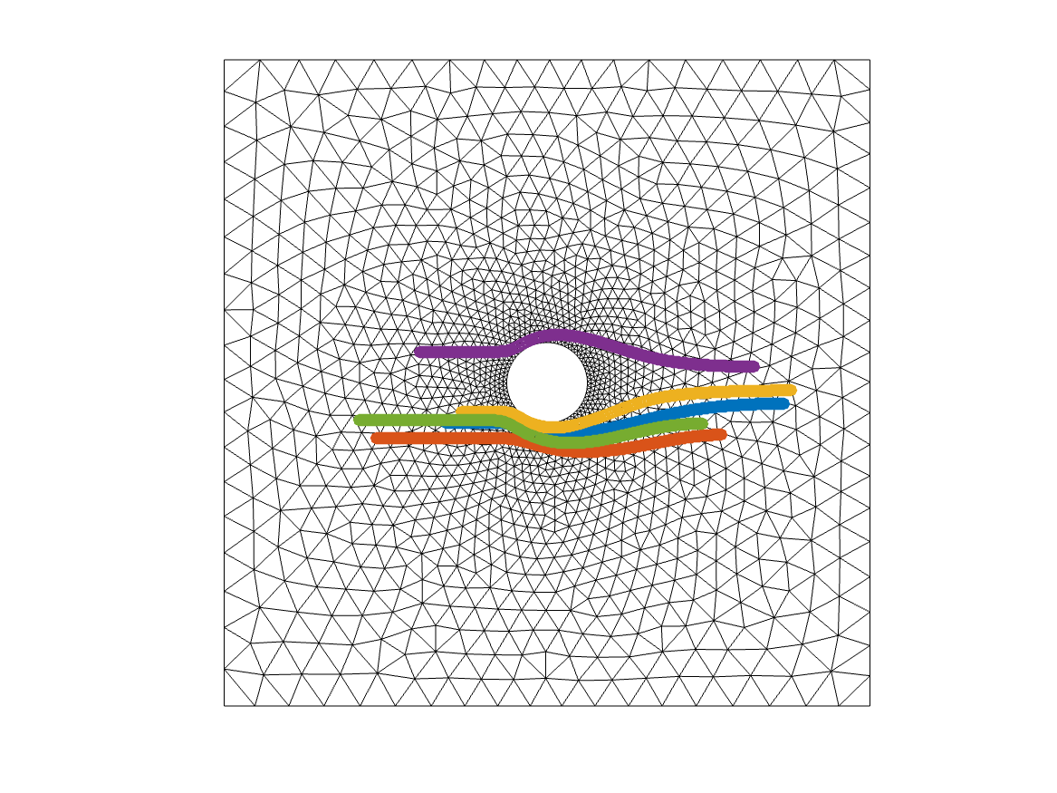
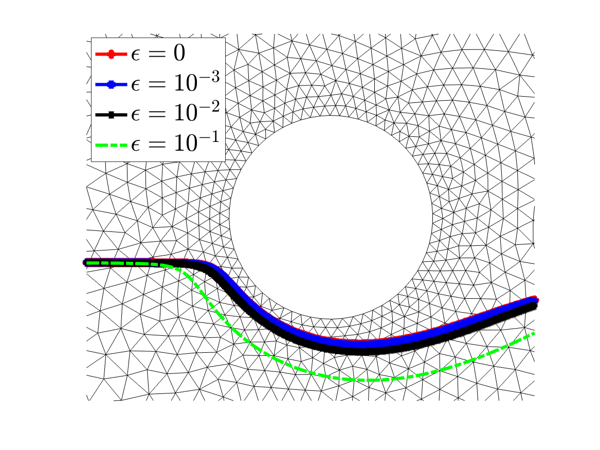
Figure 2 shows the performance of our method. Figure 2(a) shows the behavior of the error for several values of : as we increase in (19), we introduce an increasing bias in the formulation that prevents convergence to the target density. Figure 2(b) compares the deformed point cloud at the final time for with the “target” point cloud generated using : we observe that the results are extremely satisfactory for this model problem. Figure 2(c) shows the behavior of select trajectories, while Figure 2(d) shows the behavior of a select particle for several values of : we notice that, as we increase , the particle moves away from the cylinder due to the effect of the repulsive force.
4.2 Point-set registration across a cylinder
4.2.1 Problem setting
We consider the problem of continuously deforming the point cloud to match the target point cloud . We consider the same domain of the previous example and we define
| (22) |
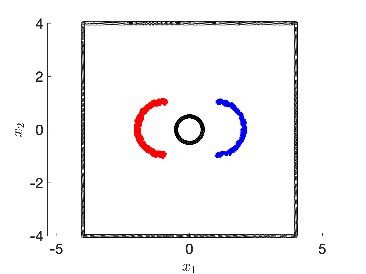
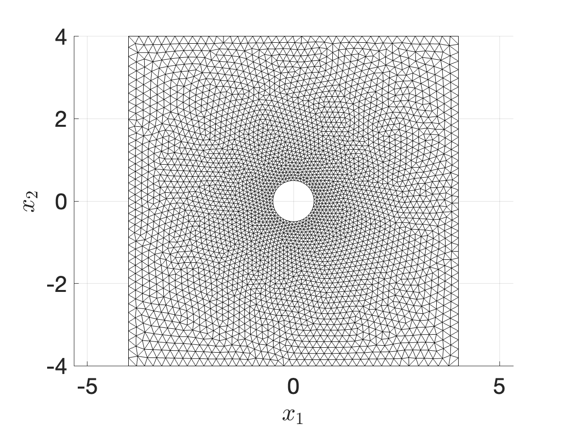
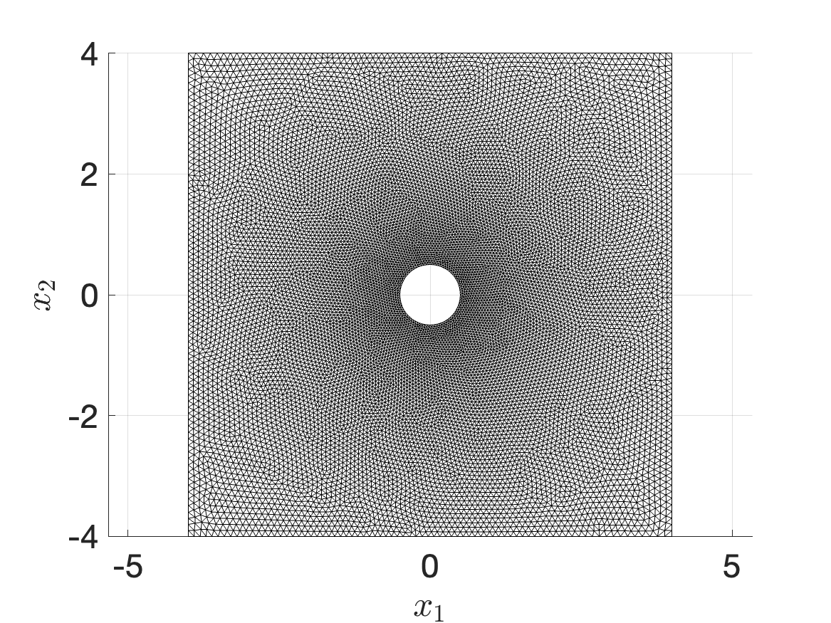
where , , , and . Figure 3(a) shows the reference and the target point clouds. We consider two distinct discretizations of increasing size. The coarse discretization features a P2 FE mesh with degrees of freedom and time steps; the fine discretization features a P3 FE mesh with degrees of freedom and time steps. In both cases, we integrate the system in the time interval and we consider the non-uniform time grid (21).
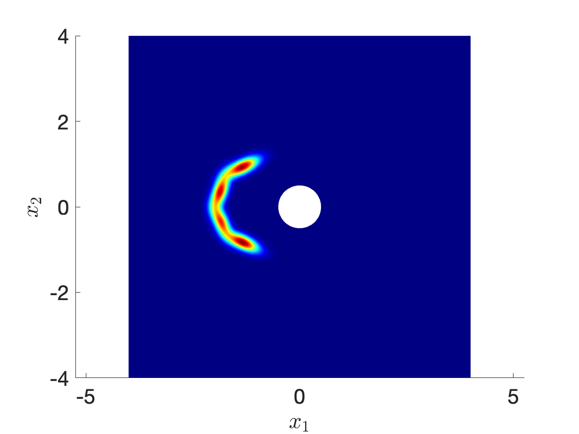
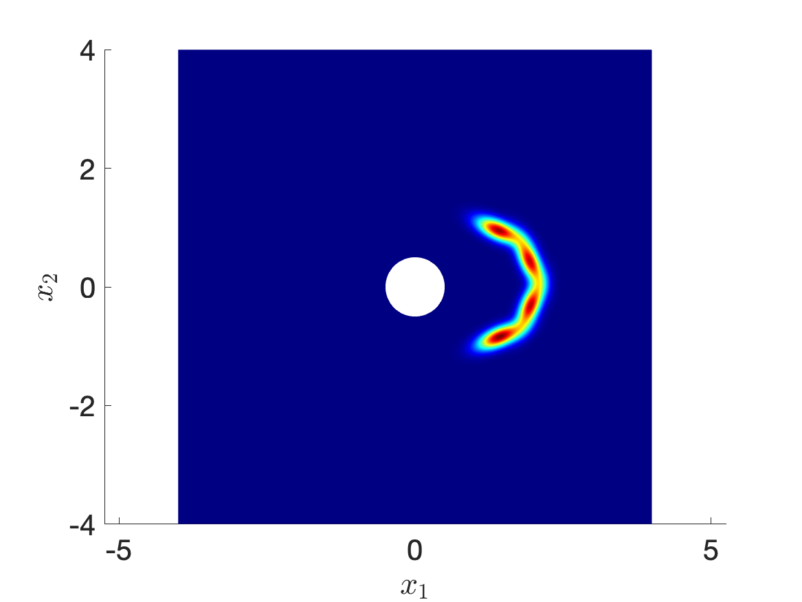
We rely on the unregularized potential (i.e., in (19)). We compare the ODE method based on forward Euler time integration with the GF method. We also run simulations for the ODE method with RK2 time integration with two time steps per time interval: since the results of the latter are comparable with the ones of the ODE method, they are not reported below. We model the point clouds (22) using two GMMs with four components — we recall that the number of components is selected by maximizing the AIC criterion. Figures 3(b) and (c) show the GMM densities that are obtained by the learning procedure.
4.2.2 Results
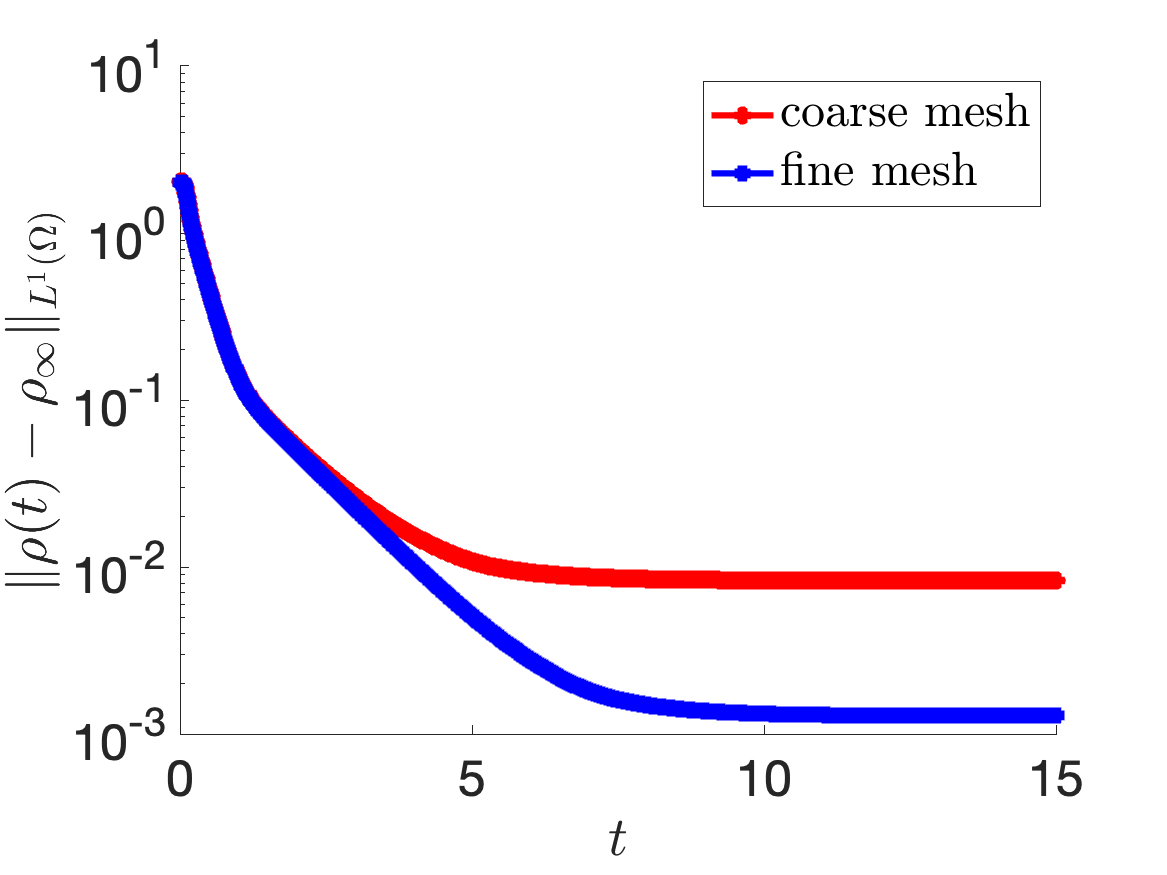
Figure 4(a) shows the behavior of the error over time for the two discretizations; Figures 4(b) and (c) show the two FE meshes. As expected, the error in the target density decreases as we increase the size of the mesh.
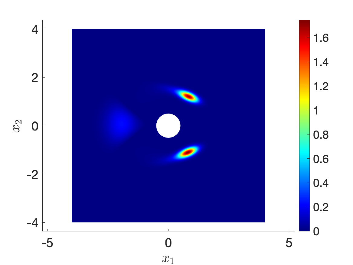
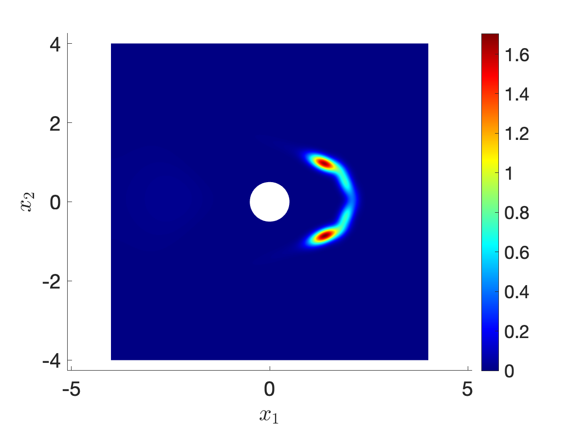
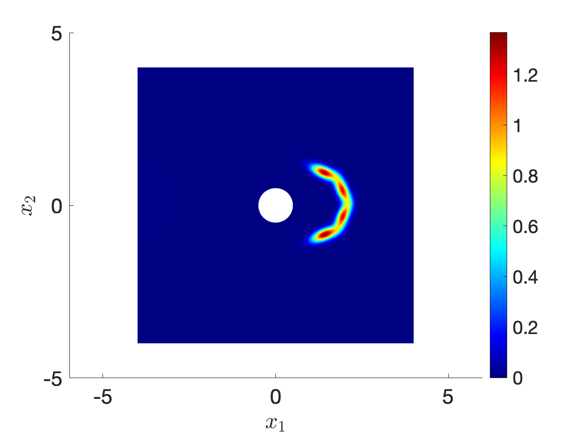
Figures 5(a), (b) and (c) show the behavior of the solution to (14) for three time instants. As expected, we notice that the solution is symmetric with respect to the cylinder. We further notice that for small time steps the solution has three peaks: the majority of the mass — corresponding to the top and the bottom peaks at — rapidly goes through the cylinder, while a small portion of the mass — corresponding to the weaker peak on the left of the cylinder at — reaches the target density later.
Figures 6 and 7 show the behaviors of the point clouds for the two particle integration methods discussed in section 3. The results correspond to the fine discretization. Interestingly, the qualitative behavior of the two methods is significantly different, particularly for small values of : in the ODE method the point cloud is nearly split in two parts at and all the points proceed towards the target cloud with similar speeds; instead, in the GF method, we can clearly identify three clusters whose elements move towards the target cloud with different speeds. The latter behavior appears to be more consistent with the results for the density in Figure 5.
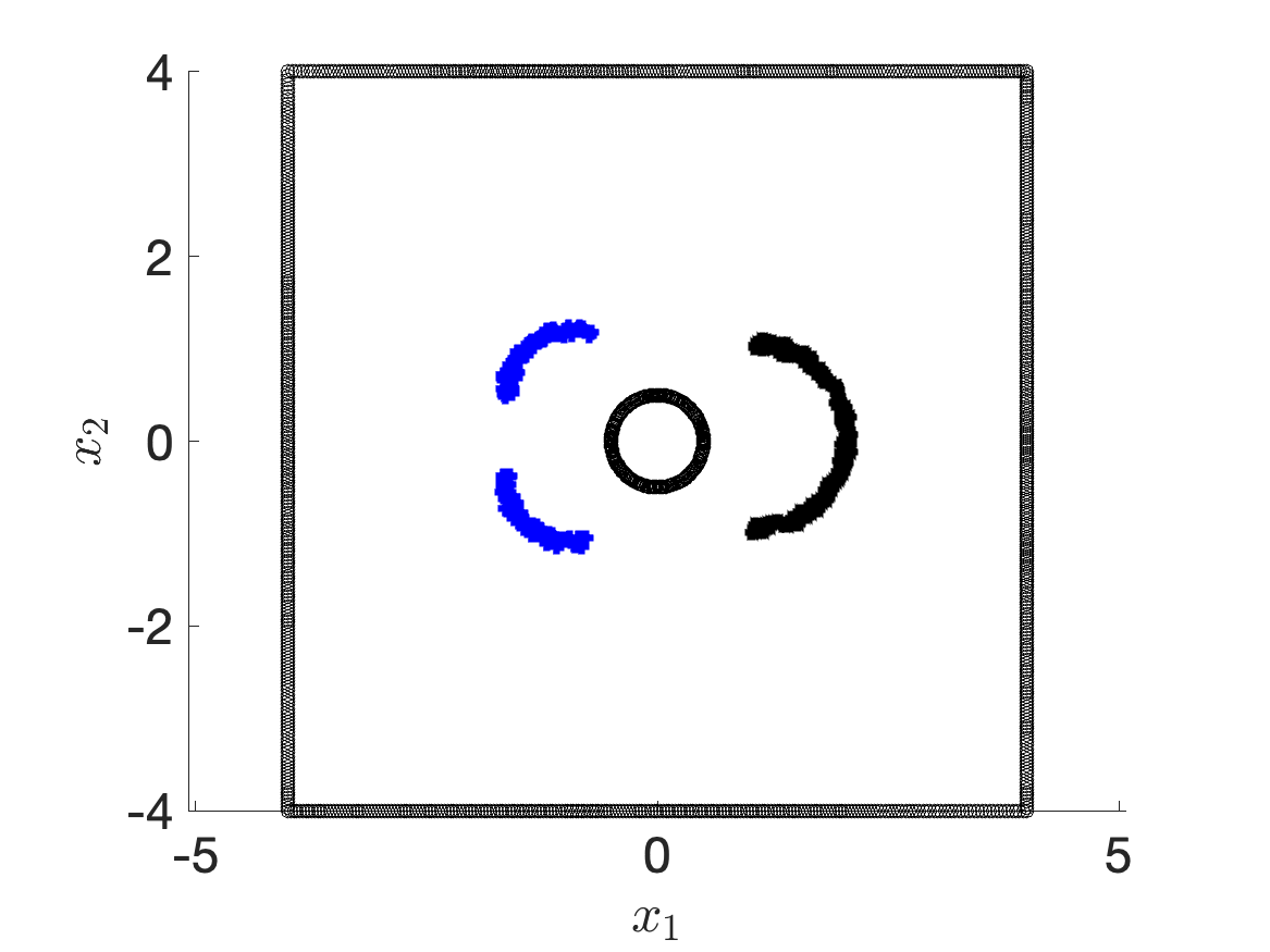
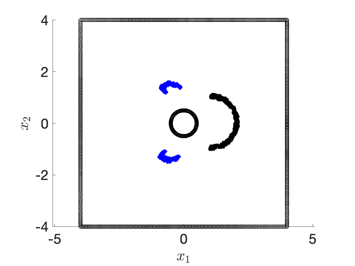
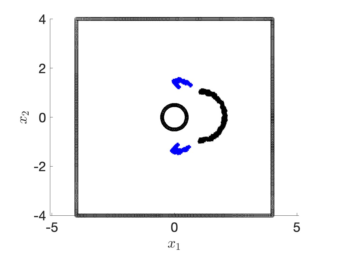
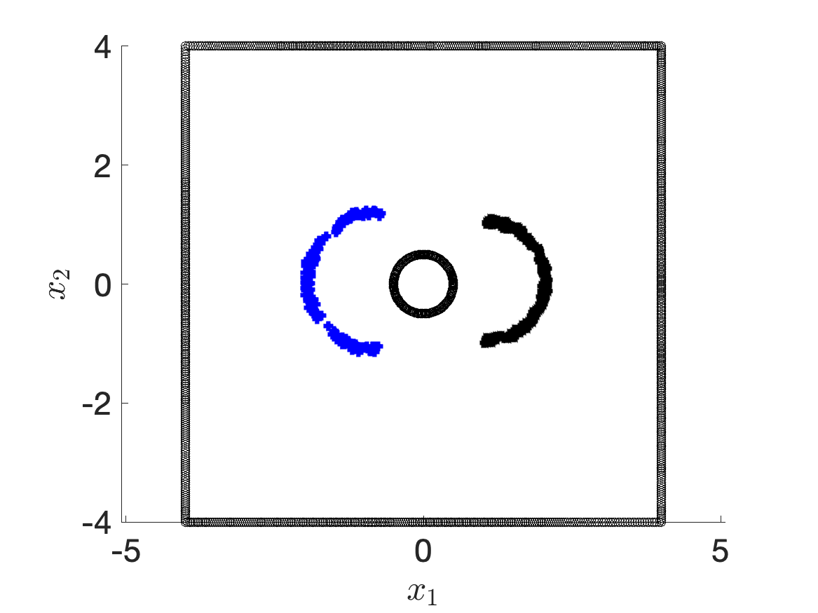
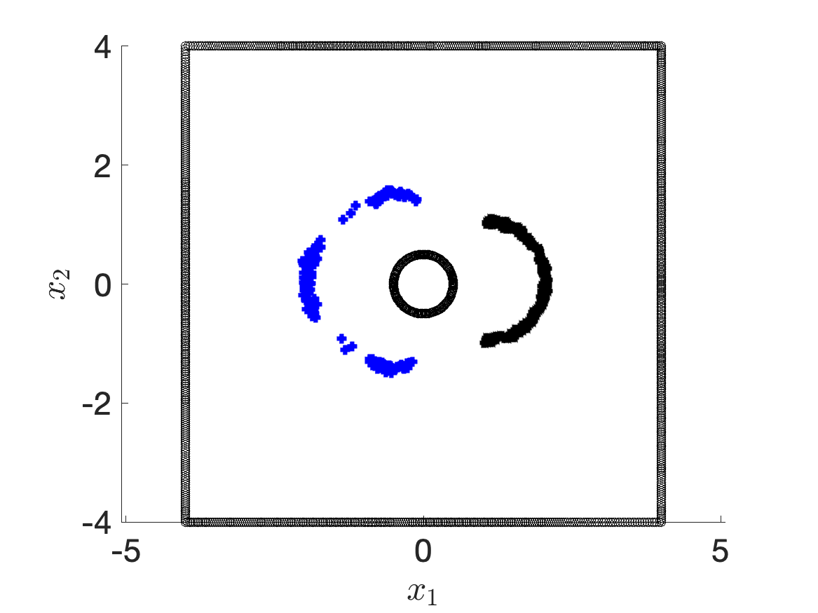
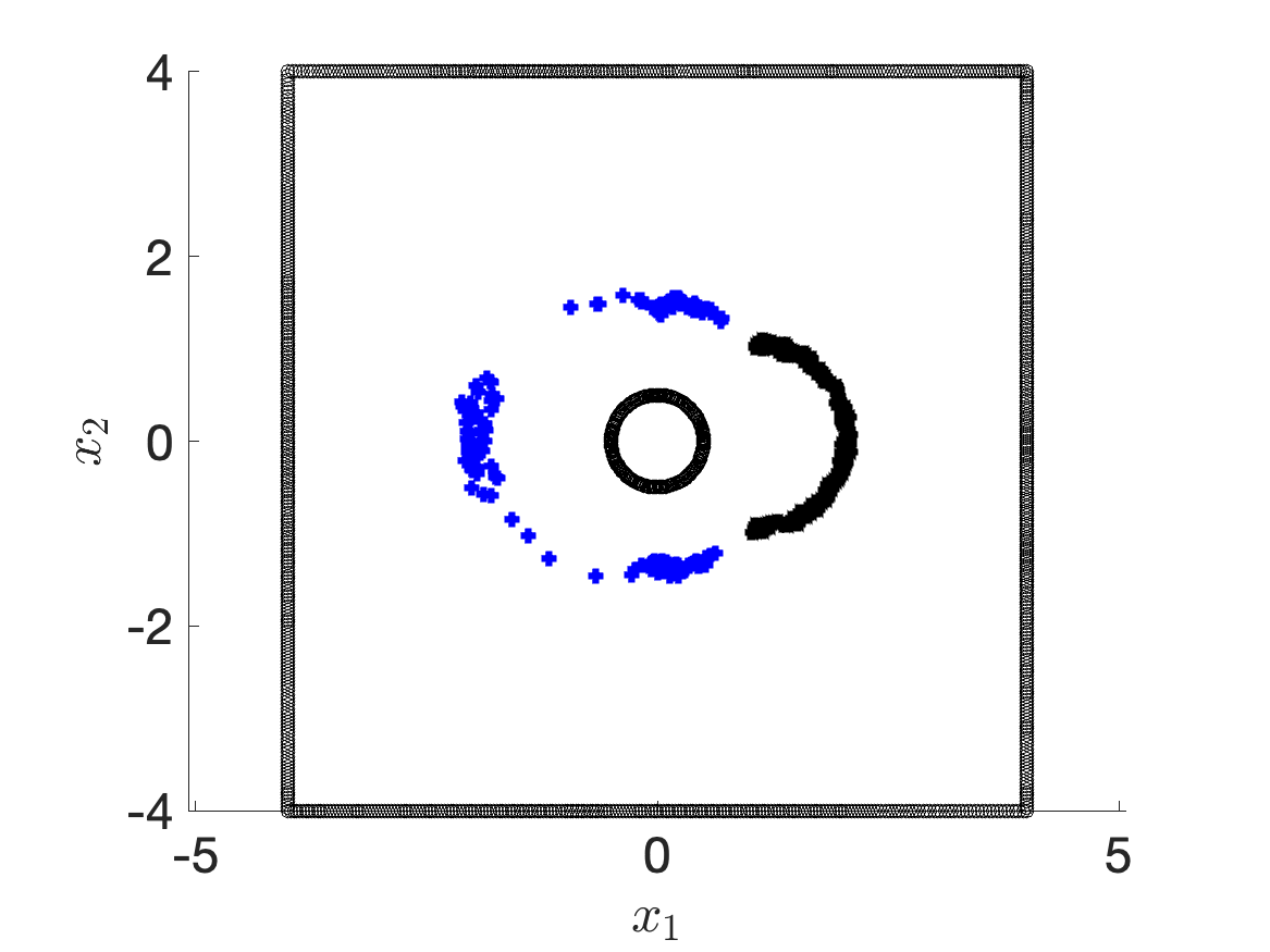
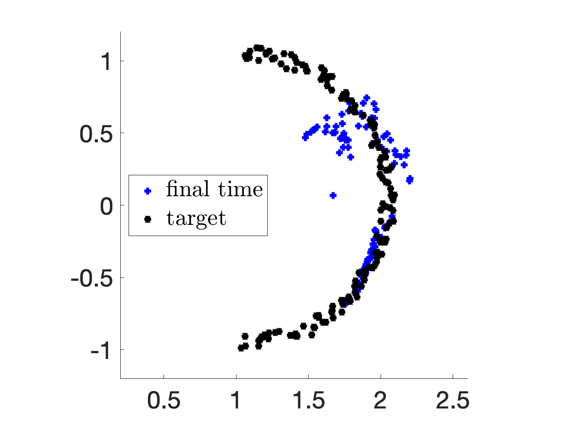
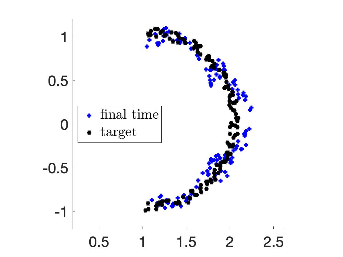
Figure 8 compares the point clouds obtained with the two methods at the final time. We notice that the ODE method does not provide satisfactory results for this test case, while the GF method is significantly more accurate.
5 Conclusions and perspectives
We developed a PSR method for the interpolation of point clouds in bounded domains based on the Fokker Planck equation. Our method relies on GMMs for density estimation and on a standard (Eulerian) discretization of the FP equation for the evaluation of the density. We also proposed two distinct strategies for the estimation of the trajectories of the particles, which are both rigorously justified by the analysis of section 2.
The numerical experiments of section 4 showed the potential of the method for PSR. The regularized potential (19) provides a simple yet effective way to control the distance of the particles from the boundaries at all times; furthermore, in both numerical experiments, the convergence to the target distribution is rapid and monotonic. As regards the motion of particles, the results of section 4.2 clearly showed the superiority of the GF approach based on the solution to a linearized OT problem over the ODE approach based on the explicit integration of the characteristics.
Despite the linearity of the equation, the solution to (4) using the FE method on a fixed grid is expensive and demands further investigations. We shall devise a specialized solver for the FP equation with emphasis on the accurate approximation of the particles’ dynamics. Specifically, we plan to consider (i) adaptive time stepping schemes and (ii) adaptive spatial discretizations to reduce the overall costs: we expect to borrow ideas from deterministic particle methods for the FP equation [16, 17].
Appendix A Proofs
A.1 Proof of Theorem 2.1
Proof.
First statement. We observe that
| (23) |
To prove (23), we notice that is a global minimum of in and . If we define the set , we find
then, exploiting (23) with , we find
which proves .
Let satisfy . If we denote by and , we find
Notice that : since is convex, recalling Jensen’s inequality, we must have that is constant, which implies that a.s.. ∎
Proof.
Second statement. It suffices to show an example for which . Towards this end, consider and
By straightforward calculations, we find and . ∎
Proof.
Third statement. We define . Since the function is strictly convex for any , we have
furthermore, the latter holds with equality if and only if . Recalling the expression of the KL divergence, we obtain the desired result. ∎
Proof.
Fourth statement. See [6, Theorem 3]. ∎
A.2 Proof of Theorem 2.2
- 1.
- 2.
-
3.
Recalling notation introduced in (2), since a.e., we find that
Provided that is strictly positive and , we have that : we have indeed
where in the second inequality we used the identity that is valid for all . Therefore, since for all , we find that the KL divergence is monotonically-decreasing and uniformly bounded. Exploiting the Pinsker’s inequality, we also find that is uniformly bounded. Then, we can apply Theorem 2.3 in [1] to conclude that in for .
- 4.
References
- [1] N. J. Alves, J. Skrzeczkowski, and A. E. Tzavaras. Strong convergence of sequences with vanishing relative entropy. arXiv preprint arXiv:2409.16892, 2024.
- [2] Y. Brenier. Polar factorization and monotone rearrangement of vector-valued functions. Communications on pure and applied mathematics, 44(4):375–417, 1991.
- [3] A. N. Brooks and T. J. Hughes. Streamline upwind/Petrov-Galerkin formulations for convection dominated flows with particular emphasis on the incompressible Navier-Stokes equations. Computer methods in applied mechanics and engineering, 32(1-3):199–259, 1982.
- [4] S. Cucchiara, A. Iollo, T. Taddei, and H. Telib. Model order reduction by convex displacement interpolation. Journal of Computational Physics, 514:113230, 2024.
- [5] C. W. Fox and S. J. Roberts. A tutorial on variational Bayesian inference. Artificial intelligence review, 38:85–95, 2012.
- [6] G. L. Gilardoni. On Pinsker’s and Vajda’s type inequalities for Csiszár’s -divergences. IEEE Transactions on Information Theory, 56(11):5377–5386, 2010.
- [7] R. M. Gray. Entropy and information theory. Springer Science & Business Media, 2011.
- [8] T. Hastie, R. Tibshirani, and J. Friedman. The Elements of Statistical Learning. Springer Series in Statistics. Springer New York Inc., New York, NY, USA, 2009.
- [9] A. Iollo and D. Lombardi. Advection modes by optimal mass transfer. Physical Review E, 89(2):022923, 2014.
- [10] A. Iollo and T. Taddei. Mapping of coherent structures in parameterized flows by learning optimal transportation with Gaussian models. Journal of Computational Physics, 471:111671, 2022.
- [11] R. Jordan, D. Kinderlehrer, and F. Otto. The variational formulation of the Fokker–Planck equation. SIAM journal on mathematical analysis, 29(1):1–17, 1998.
- [12] S. Kullback. Information theory and statistics. Courier Corporation, 1997.
- [13] I. Mozolevski, E. Süli, and P. R. Bösing. hp-version a priori error analysis of interior penalty discontinuous Galerkin finite element approximations to the biharmonic equation. Journal of Scientific Computing, 30(3):465–491, 2007.
- [14] E.-M. Ouhabaz. Analysis of heat equations on domains. Princeton University Press, 2009.
- [15] G. Peyré, M. Cuturi, et al. Computational optimal transport: With applications to data science. Foundations and Trends® in Machine Learning, 11(5-6):355–607, 2019.
- [16] G. Russo. Deterministic diffusion of particles. Communications on Pure and Applied Mathematics, 43(6):697–733, 1990.
- [17] G. Russo. A deterministic vortex method for the Navier-Stokes equations. Journal of Computational Physics, 108(1):84–94, 1993.
- [18] S. Salsa. Partial differential equations in action, volume 1. Springer, third edition, 2016.
- [19] F. Santambrogio. Optimal transport for applied mathematicians. Birkäuser, NY, 55(58-63):94, 2015.
- [20] Y. Song and S. Ermon. Generative modeling by estimating gradients of the data distribution. Advances in neural information processing systems, 32, 2019.
- [21] T. Taddei. A registration method for model order reduction: data compression and geometry reduction. SIAM Journal on Scientific Computing, 42(2):A997–A1027, 2020.
- [22] N. G. Van Kampen. Stochastic processes in physics and chemistry, volume 1. Elsevier, 1992.