Stochastic Learning of Non-Conjugate Variational Posterior for Image Classification

Abstract

Large scale Bayesian nonparametrics (BNP) learner such as stochastic variational inference (SVI) can handle datasets with large class number and large training size at fractional cost. Like its predecessor, SVI rely on the assumption of conjugate variational posterior to approximate the true posterior. A more challenging problem is to consider large scale learning on non-conjugate posterior. Recent works in this direction are mostly associated with using Monte Carlo methods for approximating the learner. However, these works are usually demonstrated on non-BNP related task and less complex models such as logistic regression, due to higher computational complexity. In order to overcome the issue faced by SVI, we develop a novel approach based on the recently proposed variational maximization-maximization (VMM) learner to allow large scale learning on non-conjugate posterior. Unlike SVI, our VMM learner does not require closed-form expression for the variational posterior expectatations. Our only requirement is that the variational posterior is differentiable. In order to ensure convergence in stochastic settings, SVI rely on decaying step-sizes to slow its learning. Inspired by SVI and Adam, we propose the novel use of decaying step-sizes on both gradient and ascent direction in our VMM to significantly improve its learning. We show that our proposed methods is compatible with ResNet features when applied to large class number datasets such as MIT67 and SUN397. Finally, we compare our proposed learner with several recent works such as deep clustering algorithms and showed we were able to produce on par or outperform the state-of-the-art methods in terms of clustering measures.

I Introduction

Bayesian nonparametrics (BNP) is widely used in image processing, video processing and natural language processing. A common task in BNP also known as model selection is to automatically estimate the number of classes to represent an unlabelled dataset as well as cluster samples (or label) accordingly. A widely used BNP is the Variational Bayes Dirichlet process mixture (VB-DPM) [1, 2, 3, 4, 5].

In the past, approximate learning for BNPs is mainly based on Variational Inference (VI) where it iteratively repeats its computational task (or algorithm) on the entire dataset, also known as batch learning [6, 7, 8, 9, 10, 11, 12, 13, 14]. Today, most large scale BNP learners such as stochastic variational inference (SVI) [2, 15, 16, 17] repeats its computational task on a smaller set of randomly drawn samples (or minibatch) each iteration. This allows the algorithm to “see” the entire dataset especially large datasets when sufficient iterations has passed. However, past VI are mostly limited to conjugate posteriors due to the mathematical convenience of available closed-form solution.

Fortunately, recent studies demonstrate that this is not always the case. Several recent works turn to Monte Carlo gradient estimator (MC) to approximate the expectation (or gradient) of the non-conjugate posterior. Some notable works in this area include the black box VI [18], VI with stochastic search [19], the stochastic gradient variational Bayes [20] and the stochastic gradient Langevin dynamics [21]. There are two advantages. Firstly, there is no need to constrain the learning of variational posteriors expectation to closed-form solution. Secondly, MC approximated posterior approaches true posteriors (closed-form VI are true solution of approximated posterior). However, MC algorithms come at an expensive cost since it require generating samples from the approximated posteriors. Moreover, such works are usually confined to binary classifier such as logistic regression [21, 22, 19, 18] or Gaussian assumptions [23, 20] and mainly demonstrated on datasets with smaller class numbers such as MNIST or UCI repository. Thus, the MC approach described above are more suitable to relatively simpler parameter inference problems.

Due to the recent paradigm shift towards deep ConvNet (CNN) [24, 25], generative networks [20, 26] and deep clustering algorithms [27, 28, 29, 30] it is very rare to find newer works following the pipeline of SVI since CNN and generative networks do not specifically deal with model selection or unsupervised class prediction.

The main problems faced by SVI and MC:

1) SVI - The approximate posterior must come from the conjugate exponential family e.g. Gaussian-Gamma.

2) MC - More expensive, since method require generating samples from the approximated posteriors.

There are three main contributions in this work:

1) A new BNP model - We propose the Pitman-Yor process generalized Gaussian mixture model (PYPM) for model selection, as it has interesting properties: it contains approximate posteriors that are conjugate, non-conjugate and discrete. Ideal case study showing the differences between learning conjugate and non-conjugate posteriors.

2) Non-conjugate posterior - Unlike SVI, we do not require closed-form expression for the variational posterior expectatations. Unlike MC, we do not require generating samples of the approximate posterior. We only take the MAP estimate of approximate posteriors for learning similarly in [22].

3) Stochastic optimization - Inspired by Adam, we use decaying stepsize on both gradient and ascent direction for approximate posterior learning.

We test the performance of our proposed learner on large class number datasets such as MIT67 and SUN397. Due to using deep ConvNet features (ResNet18), we also reported better results than most recent literature baselines.

This paper is organized as follows: Firstly, we recall VMM [31, 32] for conjugate posteriors and apply it to the conjugate posterior in the PYPM model. Next, we extend VMM for learning non-conjugate posterior in PYPM. We further improve this learning with an Adam like stochastic optimization. We then present an algorithm that iteratively learns all the hidden variables of PYPM in a typical VI fashion. Lastly, we perform a study on several datasets including the more challenging MIT67 and SUN397 to evaluate the performance of our proposed method and enhancements. Finally, we include comparison with latest published works citing the datasets we use.

I-A Related Works

Our work falls outside the SVI and the MC category. In MC, Monte Carlo gradient estimate such as in [19, 33] is used for learning non-conjugate posterior. In our work, we use Maximum a posteriori (MAP) estimate for simplicity. A similar MAP technique was also recently discussed in [22], supporting the use of gradient ascent for learning approximate posterior. However, the authors mainly use gradient ascent with constant stepsize for learning. Furthermore, their problem is directed at optimizing this constant stepsize for posterior learning.

SVI do not involve actual computation of gradient ascent. Instead, SVI parameters are found by first learning variational posteriors using variational expectation-expectation (VEE) a.k.a closed-form coordinate ascent [34] but on minibatches and finally obtained by performing a weighted average between the values computed currently and from the previous iteration. The weights follow a decay that gradually give preference to earlier VEE computed values. SVI is recently demonstrated on BNP models with conjugate posterior such as the hierarchical Dirichlet Process topic model [2] and on large datasets as large as 3.8M samples and 300 classes. On the other hand, MC methods use gradient ascent to perform learning. The key idea is to treat the gradient of the approximate posterior as expectation for learning.

II Background: Bayesian Nonparametric Model and Learning

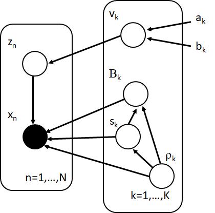
Figure 1: Pitman-Yor Process (generalized Gaussian) Mixture

Before introducing our proposed learner for model selection later on, we first introduce a well known model, the Dirichlet process mixture (DPM) [31, 34]. For the last decade, DPM has mainly found application in model selection of classification datasets such as UCI, MNIST, text classification, object recognition, scene recognition and etc. The model selection aspect of DPM actually comes from Dirichlet process while the distribution of each model comes from a Gaussian component of DPM. A more interesting variant of DPM is the Pitman-Yor Process mixture (PYPM) in Figure 1.

II-A Pitman-Yor Process generalized Gaussian Mixture (PYPM)

Another view of DP is to consider it as a specific case of the Pitman-Yor process [35]. The Pitman-Yor process is controlled by a two parameter Beta distribution where the parameters are$\begin{array}[]{c}a_{k}=1-d\end{array}$ and $b_{k}=\alpha_{0}+kd$ for $0\leq d<1$

$$Beta(v_{k};a_{k},b_{k})\propto v_{k}^{\left(a_{k}-1\right)}\left(1-v_{k}\right)^{\left(b_{k}-1\right)}$$ (1)

If we set $d=0$ in the above expression then Pitman-Yor process reduces back to the Dirichlet process.

We now turn to the definition of the mixture components as illustrated in Figure 1. For the purpose of highlighting the importance of this work (i.e. when closed form coordinate ascent [34, 2] cannot conveniently work) we introduce a variant of Gaussian mixture model (GMM) that exist outside the exponential family distribution. The generalized Gaussian distribution (GGD) is a versatile 3 parameters model with mean, shape and scale parameters $\left\{B,s,\rho\right\}$. It can model non-Gaussianity assumption for datasets. The GGD pdf is defined as follows

$$\mathcal{GGD}(x|B,s,\rho)\propto\exp\left(-\left|\frac{x-B}{s}\right|^{\rho}\right)$$ (2)

In GGD, cluster mean is now denoted $B=\left\{B_{k}\right\}_{k=1}^{K}\in\mathbb{R}{}^{D}$ and we have two new hidden variables, shape and scale. They are denoted $s=\left\{s_{k}\right\}_{k=1}^{K}\in\mathbb{R}{}^{D}$ and $\rho=\left\{\rho{}_{k}\right\}_{k=1}^{K}\in\mathbb{R}{}^{D}$ respectively. Specific cases of GGD are the Gaussian PDF $\left(s=\sqrt{2},\rho=2\right)$ and Laplacian PDF $\left(s=\sqrt{2},\rho=1\right)$. Although, the GGD can be solved by the method of moments for $s$ and $\rho$, there is no closed-form parameter estimation for GGD when $B$ is non zero centered. In this work, we are only interested in exploring a new non-conjugate form to replace GMM. Hence for functionality, we limit our learning to $B$, while fixing the parameters $s,\rho.$

The joint probability of PYPM in Figure 1 can be depicted as $p(x,B,z,v)=p(x\mid B,z)p(B)p(z\mid v)p(v)$. The observation is denoted $x=\left\{x_{n}\right\}_{n=1}^{N}\in\mathbb{R}{}^{D}$. The cluster assignment is denoted $z=\left\{z_{n}\right\}_{n=1}^{N}$ where $z_{n}$ is a $1-of-K$ binary vector, subjected to $\sum_{k=1}^{K}z_{nk}=1$ and $z_{nk}\in\left\{0,1\right\}$. We summarize the distribution of each term in PYPM as follows

$$\begin{array}[]{c}x\mid B,z\sim\mathcal{GGD}\left(B_{k}\right){}^{z_{nk}}\\ B\sim\mathcal{N}\left(m_{0},\lambda_{0}\right)\\ z_{nk}\mid v_{k}\sim Mult\left(\pi_{k}\right)\\ \nu_{k}\sim Beta(a_{k},b_{k})\end{array}$$ (3)

II-B Variational Inference

A joint distribution (e.g. PYPM) can be marginalized as $p(x)=\int p(x\mid\theta)p(\theta)d\theta$. Variational inference [11] decompose the marginal distribution as $\ln p(x)=\mathcal{L}+D_{KL}$ where $\mathcal{L}$ is a lower bound on the joint distribution between observed and hidden variable and $D_{KL}$ is the Kullback-Leibler divergence of the approximate from the true posterior. They are defined as $\mathcal{L}=\int q(\theta)\ln\left(\frac{p(x,\theta)}{q(\theta)}\right)d\theta$ and $D_{KL}=-\int q(\theta)\ln\left(\frac{p(\theta|x)}{q(\theta)}\right)d\theta$. A tractable distribution $q(\theta)$ (also known as variational posterior distribution) is used to compute $\mathcal{L}$ and $D_{KL}$. When $q(\theta)=p(\theta|x)$, the $D_{KL}$ term is removed and $\mathcal{L}=\ln p(X)$. After some re-arrangement on $\mathcal{L}$, we obtain an expression, $\ln q(\theta_{j})=E_{i\neq j}\left[\ln p(x\mid\theta_{i})p(\theta_{i})\right]+const.$ where $i\neq j$ refers to $\theta_{i}\neq\theta_{j}$. We refer to $\ln q(\theta_{j})$ as the variational log-posterior (VLP) distribution. The next goal in variational inference is on how to update VLP. We refer to Table 12 to summarize some of the definitions used in this section.

II-C Variational Maximization-Maximization

The problem of learning VLP arise from the intractable integral of the expectation function, $E\left[\theta_{j}\right]=\int\theta_{j}\,q(\theta_{j})\,d\theta_{j}$. Variational Expectation-Expectation (VEE) algorithm [10, 2, 34, 11, 31] (or closed-form coordinate ascent) avoids computing this integral by exploiting statistical moments associated with $q(\theta_{j})$. However, $q(\theta_{j})$ must come from the exponential family since only statistical moments from this family are well defined.

Instead, the Variational Maximization-Maximization (VMM) algorithm [31, 32] directly computes the VLP expectation or integral using MAP estimation i.e. $E\left[\theta_{j}\right]=\arg\max_{\theta_{j}}\;\ln q(\theta_{j})$. Since $q(\theta)=\frac{\exp\left(\ln q(\theta_{j})\right)}{C}$, for MAP estimation the denominator constant can be ignored. For symmetrical distribution, the MAP of VLP has the same objective as the expectation of VLP. We summarize VMM in Algo. 1 and show an example of using VMM in section 3.

Define the VLPs for each hidden continuous variable $\theta_{j}$ for $j=1,...,J$. For each iteration until converges, update each VLP in turn while fixing the others. The VLPs are updated by taking the expectation of each VLP as follows:

1) First take the MAP estimate of $\ln q(\theta_{j})$, to approximate the expectation of the VLP

$$\begin{array}[]{c}E\left[\theta_{j}\right]=\int\theta_{j}\,q(\theta_{j})\,d\theta_{j}\\ =\arg\max_{\theta_{j}}\;\ln q(\theta_{j})\end{array}$$

2) Next, re-arrange a closed-form expresssion, $\hat{\theta_{j}}$ after setting

$$\hat{\theta_{j}}\rightarrow\nabla_{\theta_{j}}\ln q(\theta_{j})=0$$

3) Finally, let the expectation of the VLP be approximated by $\hat{\theta_{j}}$

$$E\left[\theta_{j}\right]=\hat{\theta_{j}}$$

Algorithm 1 Variational Maximization-Maximization [31]

III Problem Statement

We present the problem of learning non-conjugate VLP from a complex Bayesian model such as the Pitman-Yor process generalized-Gaussian mixture (PYPM) model. The PYPM model presented here has three hidden variables $\theta=\left\{v_{k},B_{k},z_{nk}\right\}$, each requires to be solved in a different way i.e. conjugate, non-conjugate, discrete. Firstly, we explain how conjugate VLP is learnt in the traditional way such as using VMM. Next, we state the difficulty faced when learning non-conjugate VLP using VMM.

III-A VMM Learning of Conjugate VLP

We apply the VMM of PYPM to iteratively update $\ln q(v_{k})$. Due to conjugate assumption for $\ln q(v_{k})$ i.e. Multinomial-Beta posterior, we can derive a closed-form expression denoted $\hat{v_{k}}$ below.

Using Algo. 1:

1) Take the MAP estimate of $\ln q(v_{k})$

$$\begin{array}[]{c}E\left[v_{k}\right]=\underset{v_{k}}{\arg\max}\;\ln q(v_{k})\\ =\underset{v_{k}}{\arg\max}\;\underset{z_{nk}}{E}\left[\ln p(z_{nk}\mid v_{k})+\ln p(v_{k})\right]\\ =\underset{v_{k}}{\arg\max}\;\left\{\sum_{n=1}^{N}\sum_{j=k+1}^{K}\ln\left(1-v_{k}\right)E\left[z_{nj}\right]\right.\\ \left.+\sum_{n=1}^{N}E\left[z_{nk}\right]\ln v_{k}+\left(a_{k}-1\right)\ln v_{k}+\left(b_{k}-1\right)\ln\left(1-v_{k}\right)\right\}\end{array}$$ (4)

2) After setting $\nabla_{v_{k}}\ln q(v_{k})=0$ and re-arranging the RHS in terms of $v_{k}$, we have a closed form solution for $\hat{v_{k}}$

$$\begin{array}[]{c}\nabla_{v_{k}}\ln q(v_{k})=-\frac{\sum_{n=1}^{N}\sum_{j=k+1}^{K}E\left[z_{nj}\right]}{1-v_{k}}\\ +\frac{\sum_{n=1}^{N}E\left[z_{nk}\right]}{v_{k}}+\frac{\left(a_{k}-1\right)}{v_{k}}-\frac{\left(b_{k}-1\right)}{1-v_{k}}\end{array}$$ (5)

$$\hat{v_{k}}=\frac{\sum_{n=1}^{N}E\left[z_{nk}\right]+\left(a_{k}-1\right)}{\sum_{n=1}^{N}\sum_{j=k+1}^{K}E\left[z_{nj}\right]+\left(a_{k}-1\right)+\left(b_{k}-1\right)}$$ (6)

3) Finally, we set the approximation as

$$E\left[v_{k}\right]=\hat{v_{k}}$$

In the VMM of DPM in [31], we can similarly obtain a closed form solution for a Gaussian-Gamma posterior (for cluster precision) and a Gaussian-Gaussian posterior (for cluster mean).

III-B Problem of Learning Non-Conjugate VLP

Next, we attempt using VMM to a case of non-conjugate VLP, $\ln q(B{}_{k})$ where the likelihood is generalized Gaussian distributed and prior term Gaussian distributed.

Using Algo. 1:

1) Take the MAP estimate of $\ln q(B_{k})$

$$\begin{array}[]{c}E\left[B_{k}\right]=\underset{B_{k}}{\arg\max}\;\ln q(B_{k})\\ =\underset{B_{k}}{\arg\max}\;\underset{z_{nk}}{E}\left[\ln p(x_{n}\mid B_{k},z_{nk})+\ln p(B_{k})\right]\\ =\underset{B_{k}}{\arg\max}\;\left\{-\left|\frac{x_{n}-B_{k}}{s}\right|^{\rho}E\left[z_{nk}\right]+\ln p(B_{k})\right\}\end{array}$$ (7)

2) Because the likelihood is not from the exponential family, re-arranging the gradient in terms of $B_{k}$ for $\nabla_{B_{k}}\ln q(B_{k})=0$ is difficult

$$\begin{array}[]{c}\nabla_{B_{k}}\ln q(B_{k})=\frac{\rho}{s}\left|\frac{x_{n}-B_{k}}{s}\right|^{\rho-1}sgn(\frac{x_{n}-B_{k}}{s})E\left[z_{nk}\right]\\ +\nabla_{B_{k}}\ln p(B_{k})\end{array}$$ (8)

The above requires i) a numerical approach and ii) a stochastic learner for large sample size and large class number. Both problems are the main highlights of this work and shall be discussed in detail in the next section.

IV Proposed Solution: Stochastic Learning of Non-Conjugate VLP

Previously, the goal of VMM (Table 1) is to update or learn $\ln q(\theta_{j})$ by deriving a closed-form expression for $E\left[\theta_{j}\right]$, given the VLP is a conjugate posterior. In this section, we propose a gradient ascent approach to estimate a case of non-conjugate VLP. We also seek stochastic learning, faster convergence and returning better local maxima. For the sake of brevity, we refer to $\theta$ as $\theta_{j}$ in this section.

IV-A VMM Learning of Non-Conjugate VLP

To overcome the lack of a closed-form solution for $E\left[\theta\right]$, some recent works [18, 19, 20, 21, 23, 36], propose the learning of non-conjugate VLP using Monte Carlo gradient estimate, $\nabla_{\theta}E\left[f(\theta)\right]\approx\frac{1}{S}\sum_{s=1}^{S}f(\theta)\nabla_{\theta}\ln q(\theta_{s})$ for approximation. However, this approximation is associated with large gradient variance and requiring generating posterior samples, $\theta_{s}$. A more recent work [22] proposed using constant stepsize gradient ascent for variational inference.

Similarly, we can re-express the expectation of $\ln q(\theta)$ using constant gradient ascent stepsize below (since approaching the local maximum has the same goal as maximizing the VLP globally)

$$\begin{array}[]{c}E\left[\theta\right]_{t}=\int\theta_{j}\,q(\theta_{j})\,d\theta_{j}\\ =E\left[\theta\right]_{t-1}+\eta\nabla_{\theta}\ln q(\theta)\end{array}$$ (9)

IV-B Stochastic Learning

In stochastic learning, we draw a small subset of samples (e.g. 1k samples) per iteration to update each VLP. This is more effective than taking the entire dataset (say 10k samples) for learning. In stochastic optimization [37], there is a requirement for a decaying step-size $p_{t}$ to ensure convergence in SGA as given by $\sum p_{t}=\infty$ and $\sum p_{t}^{2}<\infty$. This is to avoid SGA bouncing around the optimum of the objective function.

In SVI [2], the main goal is to obtain the “global parameter” update of conjugate VLP from its “immediate global parameter”

$$\left(\phi_{global}\right)_{t}=(1-p_{t})\left(\phi_{global}\right)_{t-1}+p_{t}\cdot\phi_{immed}$$ (10)

The “immediate global parameter” is defined as a noisy estimate and is cheaper to run since it is computed from a data point sampled each iteration, rather than from the whole data set. The decaying step-size is defined as $p_{t}=\left(\tau+t\right)^{-\kappa}$ and both $\tau$ and $\kappa$ are treated as constants. Our view of the SVI update equation above is much simpler and has little to do with SVI. Instead, we simply treat it as a weighted average between current and previous computed gradient of the VLP to ensure convergence in learning. In fact, eqn (10) is also commonly known as exponentially weighted averaging and it is a prerequisite in the optimization of “SGA with momentum”. The main difference being $p_{t}$ is a decaying term rather than fixed. Thus, we defined the decaying stepsize VLP gradient for a given minibatch of size $M$ samples at $t$ iteration as

$$W_{t}=\left(1-p_{t}\right)W_{t-1}+p_{t}\left(\frac{1}{M}\sum_{m=1}^{M}\nabla_{\theta}\ln q(\theta)\right)$$ (11)

The non-conjugate learner in eqn (9) is based on the gradient ascent approach. Since we are dealing with an approximate posterior or VLP which is assumed convex, a more superior gradient learning is the natural gradient learning. It uses Fisher information matrix $G=E\left[\nabla_{\theta}\ln q(\theta)(\nabla_{\theta}\ln q(\theta))^{T}\right]$, as the steepest ascent directional search is in Riemannian space [38]. Natural gradient learning is superior to gradient learning because the shortest path between two point is not a straight-line but instead falls along the curvature of the VLP objective [38]. Natural gradient ascent of VLP is defined as follows [39, 2]

$$\begin{array}[]{c}E\left[\theta\right]_{t}=E\left[\theta\right]_{t-1}+\eta G^{-1}\nabla_{\theta}\ln q(\theta)\end{array}$$ (12)

When we assumed each dimension is independent (spherical or diagonal VLP), we end up with the squared gradient of VLP, $G=E\left[\left(\nabla_{\theta}\ln q\left(\theta\right)\right)^{2}\right]$. For a minibatch of size $M$ samples, we introduce decaying stepsize for the squared gradient of VLP, using the identity $E\left[X^{2}\right]\geq\left\{E\left[X\right]\right\}^{2}$ as follows

$$F_{t}=\left(1-p_{t}\right)F_{t-1}+p_{t}\left(\frac{1}{M}\sum_{m=1}^{M}\nabla_{\theta}\ln q(\theta)\right)^{2}$$ (13)

The roles of the decaying stepsize gradient and squared gradient of VLP are defined below for gradient ascent

$$E\left[\theta\right]_{t}=E\left[\theta\right]_{t-1}+\eta\frac{W_{t}}{\sqrt{F_{t}}}$$ (14)

For our convenience, we name this stochastic learning of VMM as sVMM.

IV-C Motivation and Related Works

Our proposed learner, sVMM is motivated by recent SGA methods and SVI as summarized in Table 1. We briefly discuss their similarity below using the VLP case of $\ln q(\theta)$. For the sake of brevity, we refer to $g_{t}=\frac{1}{M}\sum_{m=1}^{M}\nabla_{\theta}\ln q(\theta)$ at iteration $t$.

Gradient Ascent: When we fix $p_{t}=1$ (i.e. fixed stepsize) in eqn (11) and (13), $E\left[\theta\right]_{t}$ in eqn (14) reduces to the natural gradient ascent in eqn (12). Instead of taking the inverse of $F$, we now take the inverse square root of $F$.

SVI: In Table 1, we compare eqn (11) to the update equation in SVI. We can view the closed-form estimate $\hat{\theta}$ as the immediate global parameter while $E\left[\theta\right]_{t}$ is seen as the global parameter.

Adam: Our definition of $W_{t}$ and $F_{t}$ look similar to the first and second moments $M_{t}$ and $V_{t}$ in Adam. The main difference lies in the way we define the stepsizes $p_{t}$. We adopt the stepsize defined by SVI. In Adam the decaying stepsizes (i.e. $\beta_{1}^{t}$ and $\beta_{2}^{t}$) is found in their bias correction step where $\hat{M_{t}}=M_{t}/\left(1-\beta_{1}^{t}\right)$ and vice versa for $\hat{V_{t}}$. In Adam, $\beta_{1}$ and $\beta_{2}$ are actually constant values at 0.9 and 0.999. We also use an identical expression to Adam for the gradient ascent update in eqn (14).

Methods	stepsize update	gradient ascent update
Grad. Ascent	-	$E\left[\theta\right]_{t}=E\left[\theta\right]_{t-1}+\eta g_{t}$
Natural	-	$\begin{array}[]{c}E\left[\theta\right]_{t}=E\left[\theta\right]_{t-1}+\eta\frac{g_{t}}{G}\end{array}$
Grad. Ascent
Adam	$M_{t}\propto\beta_{1}M_{t-1}+\left(1-\beta_{1}\right)g_{t}$	$E\left[\theta\right]_{t}=E\left[\theta\right]_{t-1}+\eta\frac{\hat{M_{t}}}{\sqrt{\hat{V_{t}}}+\epsilon}$
	$V_{t}\propto\beta_{2}V_{t-1}+\left(1-\beta_{2}\right)\left(g_{t}\right)^{2}$
SVI	$E\left[\theta\right]_{t}=\left(1-p_{t}\right)E\left[\theta\right]_{t-1}+p_{t}\hat{\theta}$	-
Proposed	$W_{t}=\left(1-p_{t}\right)W_{t-1}+p_{t}g_{t}$	$E\left[\theta\right]_{t}=E\left[\theta\right]_{t-1}+\eta\frac{W_{t}}{\sqrt{F_{t}}}$
(sVMM)	$F_{t}=\left(1-p_{t}\right)F_{t-1}+p_{t}\left(g_{t}\right)^{2}$

Table I: Comparison of stochastic gradient ascent techniques

The motivation for the steepest ascent direction search of VLP optimum is best explained by Riemannian geometry in [38, 2, 39] .

IV-D Convergence Analysis

We plot the curves for $\left(1-p_{t}\right)$ and $p_{t}$ to exhibit the behavior of using these stepsizes for $W_{t}$ or $F_{t}$. We set the values $\tau=1$ and $\kappa=0.5$ for $t=50$ iterations in Figure 2. We see that the curves gradually shift responsibilities from the gradual diminishing value of $p_{t}$ to the increasing value of $\left(1-p_{t}\right)$ as the number of iterations increases, for $W_{t}$ and $F_{t}$.

Recall that in the SVI update $E\left[\theta\right]_{t}=\left(1-p_{t}\right)E\left[\theta\right]_{t-1}+p_{t}\hat{\theta}$, the term $\hat{\theta}$ is defined as the closed form coordinate ascent estimate in [2]. Alternatively, $\hat{\theta}$ is computed identical to the conjugate VLP using VMM. Thus, when we let $\hat{\theta}=\nabla_{\theta}\ln q(\theta)$ at $\nabla_{\theta}\ln q(\theta)=0$ we have the following for SVI

$$E\left[\theta\right]_{t}=\left(1-p_{t}\right)E\left[\theta\right]_{t-1}+p_{t}\nabla_{\theta}\ln q(\theta)$$ (15)

For sVMM, we only discuss the case of $E\left[\theta\right]_{t}=E\left[\theta\right]_{t-1}+\eta W_{t}$. Expanding the terms inside, we have the following

$$E\left[\theta\right]_{t}=E\left[\theta\right]_{t-1}+\eta\left(1-p_{t}\right)W_{t-1}+\eta p_{t}\nabla_{\theta}\ln q(\theta)$$ (16)

Given that $\lim_{t\rightarrow\infty}\left(1-p_{t}\right)=1$ and $\lim_{t\rightarrow\infty}p_{t}=0$ in Figure 2, we can see that SVI becomes

$$\lim_{t\rightarrow\infty}E\left[\theta\right]_{t}=E\left[\theta\right]_{t-1}$$ (17)

while sVMM becomes

$$\lim_{t\rightarrow\infty}E\left[\theta\right]_{t}=E\left[\theta\right]_{t-1}+\eta W_{t-1}$$ (18)

Eqn (17) shows that SVI will reach convergence if $E\left[\theta\right]_{t-1}$ is a convex function. In eqn (18), sVMM consists of an additional term apart from $E\left[\theta\right]_{t-1}$. Specifically, $W_{t-1}$ consists of a weighted sum between $\nabla_{\theta}\ln q(\theta)$ and the previous $W_{t-1}$. Thus, as long as $\nabla_{\theta}\ln q(\theta)$ is a convex function we can sufficiently ensure that sVMM will also converge.

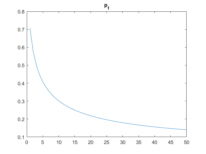
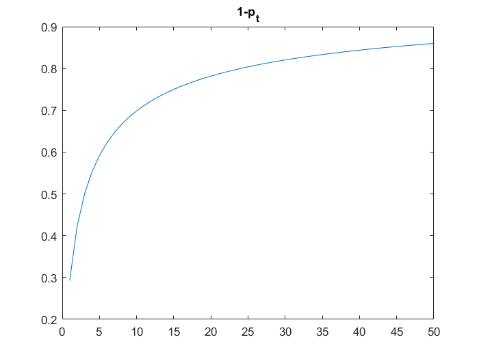
Figure 2: Behavior of stepsizes using $p_{t}=\left(1+t\right)^{-0.5}$

V Proposed Inference of PYPM

We are now ready to perform PYPM inference from a dataset given the expectation of all three VLPs (non-conjugate, discrete, conjugate) can now be solved. Essentially, we repeat the estimation of all VLP expectations using minibatch each iteration till convergence or sufficient iterations has passed. A heuristic approach to speed the algorithm is to use cluster pruning as detailed below. We summarize our proposed inference of PYPM in Algo. 2.

V-A Non-conjugate VLP

The stochastic learning of PYPM is obtained by the proposed sVMM procedure for updating the generalized Gaussian-Gaussian posterior, $E\left[B_{k}\right]_{t}=E\left[B_{k}\right]_{t-1}+\eta\frac{W_{t}}{\sqrt{F_{t}}}$, whereby $g_{t}=\frac{1}{M}\sum_{m=1}^{M}\nabla_{B_{k}}\ln q(B_{k})$. Due to requiring an initial or previous estimate, the non-conjugate VLP’s gradient is computed as follows

$$\begin{array}[]{c}\nabla_{B_{k}}\ln q(B_{k})=\frac{\rho}{s}\left|\frac{x_{n}-E\left[B_{k}\right]_{t-1}}{s}\right|^{\rho-1}sgn(\frac{x_{n}-E\left[B_{k}\right]_{t-1}}{s})E\left[z_{nk}\right]\\ -\lambda_{0}(E\left[B_{k}\right]_{t-1}-B_{0})\end{array}$$ (19)

V-B Discrete VLP

In VMM, we update the two conditional density by running through all possible $K$ states of $z_{n}$ that maximizes the posterior as below

$$\begin{array}[]{c}E\left[z_{nk}\right]=\underset{z_{nk}}{\arg\max}\;\underset{B_{k},v_{k}}{E}\left[\ln p(x_{n}\mid B_{k},z_{nk})+\ln p(z_{nk}\mid v_{k})\right]\\ =\underset{z_{nk}}{\arg\max}\;-\left\{\left|\frac{x_{n}-E\left[B_{k}\right]}{s}\right|^{\rho}\right.\\ \left.+\ln E\left[v_{k}\right]+\sum_{l=1}^{k-1}\ln(1-E\left[v_{l}\right])\right\}z_{nk}\end{array}$$ (20)

V-C Conjugate VLP

We have earlier shown the closed form VMM procedure in Section 3.1 for updating the Multinomial-Beta VLP below

$$E\left[v_{k}\right]=\frac{\sum_{n=1}^{N}E\left[z_{nk}\right]+\left(a_{k}-1\right)}{\sum_{n=1}^{N}\sum_{j=k+1}^{K}E\left[z_{nj}\right]+\left(a_{k}-1\right)+\left(b_{k}-1\right)}$$ (21)

V-D Cluster Pruning

Apart from computing the expectations, we also perform clustering ordering and pruning based on the stick-breaking construction as seen in [31]. Ideally, we want to give more emphasis to clusters with larger values of $E[v_{k}]$ to appear more frequently rather than random appearance. In order to speed up the algorithm, at the end of each iteration we run the threshold check, $E[v_{k}]<THR$ for $k=1,...,K$. When $E[v_{k}]$ does not meet the threshold, we simply discard this $k^{th}$ cluster and its associated expectations, $E[B_{k}],E[z_{nk}],E[v_{k}]$. Thus, we have one lesser cluster to compute for each case of $E[v_{k}]<THR$ occuring at the next iteration of VMM.

V-E Negative Lower Bound

A standard way to check the convergence of variational inference [34, 2] is to ensure the negative lower bound as shown below reaches saturation after sufficient iterations has passed

$$\begin{array}[]{c}\mathcal{L}\geq E\left[\ln p(x,z,B,v)\right]-E\left[\ln q(z,B,v)\right]\\ =E\left[\ln p(x\mid z,B)\right]+E\left[\ln p(B)\right]+E\left[\ln p(z\mid v)\right]\\ +E\left[\ln p(v)\right]-E\left[\ln q(z)\right]-E\left[\ln q(v)\right]-E\left[\ln q(B)\right]\end{array}$$ (22)

Each expectation function within the lower bound are computed as follows

$$\begin{array}[]{c}E\left[\ln p(x\mid B,z)\right]=\stackrel{{\scriptstyle[}}{{n}}=1]{N}{\sum}\stackrel{{\scriptstyle[}}{{k}}=1]{K}{\sum}\left\{-\left|\frac{x_{n}-E\left[B_{k}\right]}{s}\right|^{\rho}\right\}E\left[z_{nk}\right]\\ \begin{array}[]{c}E\left[\ln p(B)\right]=\sum_{k=1}^{K}-\frac{\lambda_{0}}{2}(E\left[B_{k}\right]-B_{0})^{2}\end{array}\\ \begin{array}[]{c}\begin{array}[]{c}E\left[\ln p(v)\right]=(\alpha_{0}-1)\sum_{k=1}^{K}\ln(1-E\left[v_{k}\right])\end{array}\\ \begin{array}[]{c}E\left[\ln q(z)\right]=E\left[\ln p(x\mid B,z)\right]+E\left[\ln p(z\mid v)\right]\end{array}\\ \begin{array}[]{c}E\left[\ln q(v)\right]=E\left[\ln p(v)\right]+E\left[\ln p(z\mid v)\right]\end{array}\\ E\left[\ln q(B)\right]=E\left[\ln p(x\mid B,z)\right]-E\left[\ln p(B)\right]\\ E\left[\ln p(z\mid v)\right]=\sum_{n=1}^{N}\sum_{k=1}^{K}\ln E\left[v_{k}\right]E\left[z_{nk}\right]\\ +\sum_{j=k+1}^{K}\ln\left(1-E\left[v_{j}\right]\right)E\left[z_{nj}\right]\end{array}\end{array}$$ (23)

a) Input: $x\leftarrow\left\{minibatch\right\}$

b) Output: $E\left[z_{nk}\right]$

c) Initialization: $E\left[z_{nk}\right],m_{0},\alpha_{0},\lambda_{0},a_{k},b_{k},K$

d) Repeat update until convergence,

1) non-conjugate VLP:

$$E\left[B_{k}\right]_{t}=E\left[B_{k}\right]_{t-1}+\eta\frac{W_{t}}{\sqrt{F_{t}}}$$

2) discrete VLP:

$$\begin{array}[]{c}E\left[z_{n}\right]=\underset{z_{nk}}{\arg\max}\;\ln q(z_{n})\end{array}$$

3) conjugate VLP:

$$E\left[v_{k}\right]\approx\hat{v_{k}}$$

Algorithm 2 Proposed Inference of PYPM

VI Experiments

VI-A Image Recognition Datasets

The image recognition datasets used in our experiments are detailed in Table 2. There are 3 scene and 2 digit datasets in total. The largest dataset has about over 100K images, smallest dataset is at over 4K. We split the datasets into train and test partition. Ground truth refers to the number of classes per dataset. It ranges from 15 to about 400 classes (or clusters in our case). For unsupervised learning we do not require class labels for learning our models. However, we require setting a truncation level (upper limit) for each dataset as our model cannot start with an infinite number of clusters in practice. We typically use a very large truncation value (e.g. $K=1000$ for SUN397) away from the ground truth to demonstrate that our model is not dependent on ground truth information.

For our Bayesian nonparametric task (model selection), we mainly use ResNet18 pretrained on ImageNet as our image feature extractor. The feature dimension is 512. For all datasets, we do not use any bounding box information for feature extraction. Instead, we represent the entire image using a feature vector.

For calculating our minibatch size, we approximate it by $M=sampleperclass*(gnd.truth)$, where $sampleperclass$ is typically 20 or 30 (for the datasets in this work) for sufficient statistics. In order to make the training dataset unbiased, we further assume each set of minibatch has sufficient sample draw from each class. This is necessary as some dataset have classes with 8000 samples while other classes have only 100 samples.

VI-B Evaluation Metric

We compare three criteria: i) Normalized Mutual Information, iii) Accuracy and iv) Model Selection

We use Normalized Mutual Information (NMI) and Accuracy (ACC) to evaluate the learning performance of our model. For NMI and ACC we use the code in [40]. Model refers to the model selection estimated by each approach. The definition for ACC and NMI is as follows

$$ACC=\frac{\sum_{n=1}^{N}\delta\left(gt_{n},\>map\left(mo_{n}\right)\right)}{N}$$

$$NMI=\frac{MU_{info}(gt,mo)}{\max\left(H\left(gt\right),H\left(mo\right)\right)}$$

where $gt,mo,map,\delta\left(\cdotp\right),MU_{info},H$ refers to ground truth label, model’s predicted label, permutation mapping function, delta function, mutual information and entropy respectively. Delta function is defined as $\delta(gt,mo)=1$ if $gt=mo$ and equal 0 otherwise.

We can see that for ACC it is measuring how many times the model can reproduce the same label as the ground truth on average. For NMI, it is measuring how much is the overlap or mutual information between ground truth entropy and model entropy.

VI-C Empirical Performance Evaluation

We evaluate the performance of our proposed learner for the non-conjugate VLP of PYPM using Algo. 2 shown in Table 3, 4, 5. Specifically, we consider four cases:

1) (Gau: grad) gradient ascent in eqn (9) for solving $E\left[B_{k}\right]_{t}$, with Gaussian case where $s=\sqrt{2},\rho=2$ in $\mathcal{GGD}(B,s,\rho)$

2) (Gau: mgrad) gradient ascent with decaying stepsize, $E\left[B_{k}\right]_{t}=E\left[B_{k}\right]_{t-1}+\eta W_{t}$

3) (Gau: mgrad+mdir) gradient ascent and direction, both with decaying stepsize, $E\left[B_{k}\right]_{t}=E\left[B_{k}\right]_{t-1}+\eta\frac{W_{t}}{\sqrt{F_{t}}}$

4) (Lapl: mgrad+mdir) similar to case 3 but now repeated with Laplacian case where $s=\sqrt{2},\rho=1$ in $\mathcal{GGD}(B,s,\rho)$

We consistently observe three findings: i) both grad and mgrad appear to have similar performance. ii) mgrad+mdir improves over mgrad alone by a large gain (2% to 8% improvement in terms of ACC). This gain is more significant as the dataset size increases. iii) The Laplacian model performs on par or better than the Gaussian model for all datasets.

#	Dataset	Train	Test	Trunc. Level	M.B.
1	Scene15	750	3735	50	300
2	MIT67	3350	12,270	100	1340
3	SUN397	39,700	69,054	1000	11,910
4	MNIST	60,000	10,000	50	200
5	USPS	7,291	2,007	50	200

Table II: Datasets (scene, digit) for Bayesian nonparametrics

 

  NMI ACC Model Gau: grad 0.80333 0.81901 22 Gau: mgrad 0.80328 0.81928 22 Gau: mgrad+mdir 0.81201 0.83614 21 Lapl: mgrad+mdir 0.82324 0.84391 21

Table III: Performance on Scene15

 

  NMI ACC Model Gau: grad 0.66106 0.56496 78 Gau: mgrad 0.66058 0.56487 77 Gau: mgrad+mdir 0.68546 0.60244 78 Lapl: mgrad+mdir 0.70445 0.64645 78

Table IV: Performance on MIT67

 

  NMI ACC Model Gau: grad 0.5281 0.2612 489 Gau: mgrad 0.52795 0.26151 485 Gau: mgrad+mdir 0.58226 0.34798 513 Lapl: mgrad+mdir 0.58013 0.34133 487

Table V: Performance on SUN397

VI-D Convergence via Lower Bound

In this section, we check the convergence of the learnt PYPM model on the scene recognition train datasets using the negative lower bound plots in Figure 3. For repeatability, we only illustrate three reruns for each graph. We use Algo. 2 to perform all the VLP learning of PYPM (with GGD mixture).

In the top rows (Scene15), we have 2 graphs for the Gaussian (Gau) and Laplacian (Lapl) case respectively. We observe that both methods are able to converge after 50 iterations. However, Lapl appear to saturate faster than Gau and exhibits less fluctuation after about 30 iterations.

In the middle row (MIT67), we observe Gau suffer from some fluctuation towards the end although it appears to be converging. However, Lapl appear to have lesser fluctuation than Gau towards the end.

In the bottom row (SUN397), we observe that both method have similar convergence behavior and are still gradually increasing after 50 iterations. Also, their plots have less fluctuation since the training size is larger than the other datasets.

In conclusion, both Gau and Lapl have shown to converge well after around 50 iterations of training PYPM on three datasets. When the training size increases, the fluctuation is lesser. Also, Lapl typically exhibit less fluctuation and converge faster than Gau.

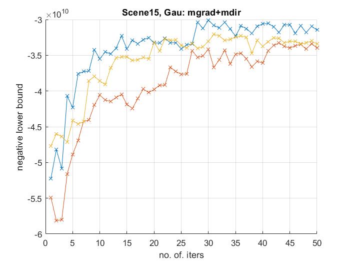
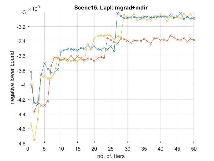
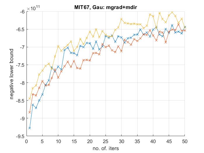
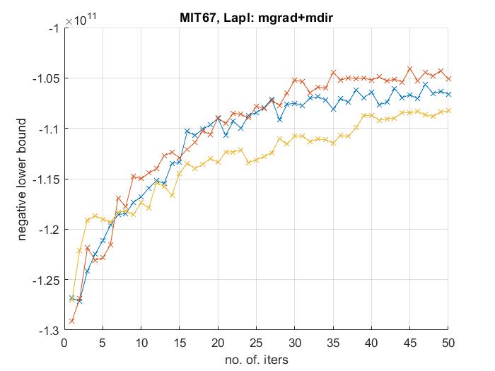
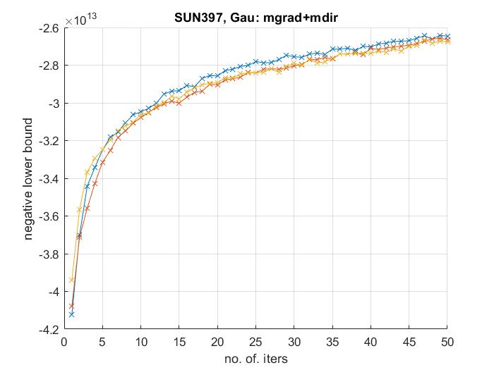
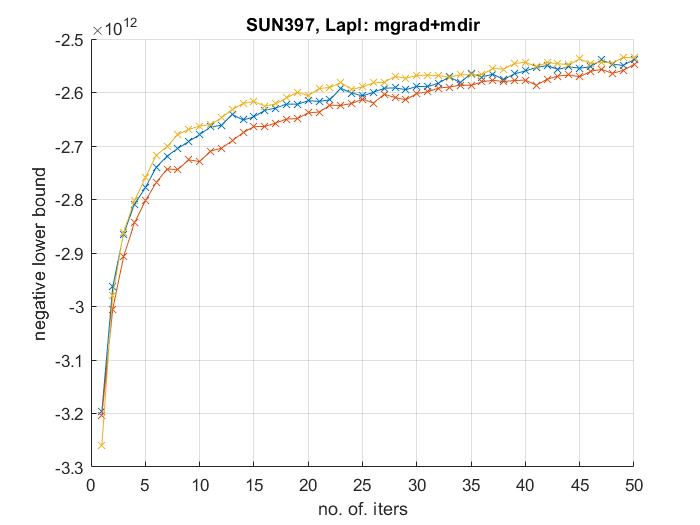
Figure 3: Negative lower bound of PYPM plots (three reruns) using the proposed inference in Algo. 2. All left columns are Gaussian case and Laplacian case of GGD on the right columns. The top row plots are for Scene15, middle row are MIT67, bottom rows are SUN397 datasets.

VII Comparison with Published Methods

We compare our work with recent works citing the datasets we use. First, we discuss the grouping of the published methods as summarized in Table 6. Also, we use 10 reruns for our proposed method and took their average (the values inside the bracket is their standard deviation).

Bayesian nonparametrics (BNP): BNPs can perform modeling and estimate the class number co-currently. These work solely consider the pursuit of advancing statistical model for large scale datasets. The methods are VMM-GMM [32], VMM-DPM [31] and OnHGD (based on SVI) [17]. Our work is also categorized under this area.

Autoencoder based clustering: A hybrid between neural network and statistical clustering, these works perform clustering in the feature space of the neural network, most of the works using autoencoder. These methods are DAEC [30], DC-Kmeans [27], DC-GMM [27], DEC [28], DBC [29] and LDPO [41]. Furthermore in some works, the clustering information may also optimize the weights update in the hidden layers. However, the statistical clustering employed here are typically the fundamentals ones such as Kmeans or GMM.

Strong Baseline: We implemented a strong baseline “SVI: DPM” to compare with our best proposed method. This baseline is the Dirichlet process Gaussian mixture and is also classified under BNP. It is implemented using the SVI update in Table 1, after obtaining the closed-form expectation of VLP as found in [31]. The remainder of the DPM algorithm is identical to the proposed DPM algorithm in [31], but without the precision VLP. We ran at least 10 reruns and took their average (the values inside the bracket is their standard deviation).

Feature: DDPM-L and OnHGD are using the 128 dimensional SIFT features. VMM-GMM, VB-DPM and VMM-DPM are using the 2048 dimensional sparse coding based Fisher vector in [42]. For LDPO, the authors use 4096 dimensional AlexNet pretrained on ImageNet. DAEC, DC-Kmeans, DC-GMM and DEC are end-to-end models that rely on the pre-trained and fine-tuned encoder to perform feature extraction. In comparison, we use the 512 dimensional ResNet18 pretrained on ImageNet.

Truncation: For LDPO, DAEC, DC-Kmeans, DC-GMM, DEC, it is fixed to the ground truth. For VMM-GMM, VB-DPM, VMM-DPM, SVI: DPM the truncation setting are identical to this work.

VII-A Scene15

In Table 7, LDPO-A-FC performs the best amongst the methods in literature but we are able to surpass LDPO-A-FC by a large margin of over 10%. For DDPM-L, VMM-GMM and VMM-DPM, there is a huge disadvantage on their results due to using handcrafted feature. BNP alone cannot overcome the discriminative advantage of deep learning feature. A standard Kmeans on deep features already yield 65% which is double in performance on VMM-DPM using a high dimensional SIFT variant.

VII-B MIT67

To the best of our knowledge, it is very rare to find any recent published works (e.g. [27, 43]) addressing datasets beyond 10 classes for image datasets. The main reason we suspect is that most recent related works rely on end-to-end learning (i.e. the encoder of the autoencoder) rather than use an ImageNet pretrained CNN for feature extraction. It is likely more difficult to train or finetune the encoder to be as discriminative as ResNet especially when there is only about 200 samples per class for MIT67 in Table 2.

In Table 8, LDPO-A-FC is almost on par with its baseline comparison using Kmeans on the larger MIT67 dataset at ACC of 37.9% vs 35.6% respectively. Our baseline method “SVI: DPM” using ResNet18 feature also perform better than LDPO-A-FC at ACC of 61.21%. We outperformed the best published method by almost double in performance using “Lapl: mgrad+mdir” at ACC of 64.47%.

VII-C SUN397

In Table 9, OnHGD applies SVI [2] (hence “On” for online) to their BNP model (HGD). They use OnHGD to learn a Bag-of-Words representation (also discussed in their batch learning counterpart [9]) for SUN397. It appears they then use a supervised learner such as Bayes’s decision rule for classification as suggested in [9]. No model selection was mentioned for SUN397 either. For SUN397, the ACC reported in OnHGD was 26.52% on SUN397. Although this is not a direct comparison, the same authors also reported an ACC of 67.34% for SUN16. In comparison, we obtained 83.37% on Scene15.

Our baseline “SVI: DPM” was able to get 39.07% on ACC compared to OnHGD of 26.52%. Our best result is “Lapl: mgrad+mdir” which was able to slightly improve the results to 40.39% on the same dataset. It may be due to the limit of our spherical Gaussian or Laplacian assumption for large class numbers. The discrepancy in Table 9 and Table 5 on the ACC and NMI of “Lapl: mgrad+mdir” (i.e. 34.8% vs 40.39%) is due to Table 9 using 100 iterations while Table 5 only uses 50 iterations due to budget constraint. The convergence of “Lapl: mgrad+mdir” is much slower for this particular dataset. Due to computational budget, we did not further check if better ACC can be obtained with 150 or 200 iterations. Also, our implementation for “SVI: DPM” faced some cluster singularity issue (cluster disappearing) when given too many iterations for SUN397. We had to stop iterations after around 15 or 20 as the cluster count may fall below 397.

VII-D MNIST

Most recent end-to-end clustering algorithms focus on digit recognition (i.e. MNIST and USPS) for experiments. Compared to MIT67 and SUN397, MNIST is a much easier dataset since the number of classes is mediocre (10 classes) and there is a large number of training images at 60k.

In Table 10, all the end-to-end methods (DAEC, DC-Kmeans/GMM, DEC, DBC) train a deep encoder (e.g. x-500-500-2000-10) as feature extractor. In comparison, we use ResNet feature directly as input to “SVI: DPM” and “Lapl: mgrad+mdir”. Table 10 shows the comparison between the published methods and ours on MNIST. For our best approach, “Lapl: mgrad+mdir”, we are able to outperform our strong baseline “SVI: DPM” as well as obtain comparable ACC and NMI to the best published result by DBC.

VII-E USPS

All the end-to-end methods (DAEC, DC-Kmeans, DEC, DBC) similarly trains a deep encoder as feature extractor. In comparison, K-means [27] using raw image pixel obtains 45.85% on ACC. For this particular dataset, we only use raw image pixel as direct input to both to “SVI: DPM” and “Gau: mgrad+mdir”. Our best result using “Gau: mgrad+mdir” consistently outperformed all published result and strong baseline again on USPS at 80.10% on ACC. Our baseline is close behind at 77.63% on ACC. The best published method DBC obtained 74.3% but it outperforms our NMI measure. We believe the reason why most end-to-end methods cannot perform better than our methods on USPS even though they are using deep encoder features while we use pixel intensity is partly due to the comparatively small training size at 7K compared to say 60K on MNIST.

#	Methods	Year	Feature	Minibatch
1	VMM-GMM [32]	2017	SC-FV	no
2	VMM-DPM [31]	2018	SC-FV	no
3	Kmeans [41]	2017	AlexNet	no
4	LDPO-A-FC [41]	2017	AlexNet	no
5	OnHGD [17]	2016	SIFT	yes
6	SVI: DPM [2]	2013	ResNet	yes
7	DAEC [30]	2013	End-to-end	yes
8	DC-Kmeans [27]	2017	End-to-end	yes
9	DC-GMM [27]	2017	End-to-end	yes
10	DEC [28]	2016	End-to-end	yes
11	DBC [29]	2018	End-to-end	yes

Table VI: Recently published methods used in this comparison

Methods	NMI	ACC
VMM-GMM [32]	0.310	0.3358
VMM-DPM [31]	0.321	0.3359
Kmeans [41]	0.659	0.65
LDPO-A-FC [41]	0.705	0.731
SVI: DPM (baseline)	0.7877 (0.0217)	0.7659 (0.0547)
Lapl: mgrad+mdir (ours)	0.8165 (0.0124)	0.8337 (0.0423)

Table VII: Comparison on Scene15

 

 

  Methods NMI ACC Kmeans [41] 0.386 0.356 LDPO-A-FC [41] 0.389 0.379 SVI: DPM (baseline) 0.6858 (0.0075) 0.6121 (0.0221) Lapl: mgrad+mdir (ours) 0.7081 (0.0103) 0.6447 (0.0218)

Table VIII: Comparison on MIT67

 

 

  Methods NMI ACC OnHGD [17] - 0.2652 SVI: DPM (baseline) 0.596 (0.004) 0.3907 (0.0079) Lapl: mgrad+mdir (ours) 0.6022 (8.2e-4) 0.4039 (0.0052)

Table IX: Comparison on SUN397

Methods	NMI	ACC
DAEC [30]	0.6615	0.734
DC-Kmeans [27]	0.7448	0.7448
DC-GMM [27]	0.8318	0.8555
DEC [28]	0.8273	0.8496
DBC [29]	0.917	0.964
SVI: DPM (baseline)	0.9233 (0.0451)	0.9348 (0.0548)
Lapl: mgrad+mdir (ours)	0.9517 (0.0343)	0.9580 (0.0573)

Table X: Comparison on MNIST

 

 

  Methods NMI ACC K-means [27] 0.4503 0.4585 DAEC [30] 0.5449 0.6111 DC-Kmeans [27] 0.5737 0.6442 DEC [28] 0.651 0.6246 DBC [29] 0.724 0.743 SVI: DPM (baseline) 0.6223 (0.005) 0.7763 (0.004) Gau: mgrad+mdir (ours) 0.6507 (8.7e-4) 0.8010 (0.0021)

Table XI: Comparison on USPS

symbol	meaning
$\ln q(\theta_{j})$	variational log-posterior (VLP)
$p(x\mid\theta_{j})$	conditional likelihood
$p(\theta_{j})$	prior distribution
$E\left[\theta_{j}\right]$	expectation of VLP
$Beta(a_{k},b_{k})$	Beta distribution
$\mathcal{GGD}(B_{k},s_{k},\rho_{k})$	generalized Gaussian distribution
$\mathcal{N}\left(B_{k}\right)$	Gaussian distribution
$Mult\left(\pi_{k}\right)$	Multinomial distribution
$\nabla_{\theta}\ln q(\theta_{j})$	gradient of VLP
$W_{t}$	gradient of VLP
	with decaying stepsize
$F_{t}$	squared gradient of VLP
	with decaying stepsize
$\eta$	learning rate
$p_{t}$	stepsize at iteration $t$
$\hat{\theta_{j}}$	closed-form estimate
$\mathcal{L}$	lower bound
$\nabla_{\theta}\mathcal{L}$	gradient of lower bound

Table XII: Symbols used and their definitions in this work

VIII Conclusion

The stochastic optimization of variational inference can be broadly categorized under two types. The first approach formulates the learning of the VLP using a gradient ascent step while the second approach rely on traditional closed-form learning. In literature, the first approach require generating Monte Carlo sample from the variational posteriors, which is not practical for large datasets such as SUN397. The second approach suffers from the constraint of requiring analytical solution for the variational posterior expectation but has reported the capability to scale up to 3.8M samples and 200 classes. In this paper, we target up to about 100K samples and 400 classes using ResNet feature pretrained on ImageNet. We try to improve on the problems faced in both approaches. We first began with the first approach and in order to make it computationally efficient, we adopted a MAP estimate in place of Monte Carlo estimate. We test our new stochastic learner on the Pitman-Yor process Gaussian mixture (PYPM) which does not have closed-form learning for the VLP. Stochastic optimization rely on decreasing step-size for guaranteed convergence. Instead, we explored using first and second order gradient inspired by Adam to achieve a faster convergence. We showed the significant performance gained in terms of NMI, ACC, model selection on large class number datasets such as the MIT67 and SUN397 with recent end-to-end deep learning related works.

References

- [1] D. M. Blei, A. Kucukelbir, and J. D. McAuliffe, “Variational inference: A review for statisticians,” Journal of the American Statistical Association, vol. 112, no. 518, pp. 859–877, 2017.
- [2] M. D. Hoffman, D. M. Blei, C. Wang, and J. W. Paisley, “Stochastic variational inference.” Journal of Machine Learning Research, vol. 14, no. 1, pp. 1303–1347, 2013.
- [3] F. Heinzl and G. Tutz, “Clustering in linear mixed models with approximate dirichlet process mixtures using em algorithm,” Statistical Modelling, vol. 13, no. 1, pp. 41–67, 2013.
- [4] A. Jara, “Theory and computations for the dirichlet process and related models: An overview,” International Journal of Approximate Reasoning, vol. 81, pp. 128–146, 2017.
- [5] L. Wang and D. B. Dunson, “Fast bayesian inference in dirichlet process mixture models,” Journal of Computational and Graphical Statistics, vol. 20, no. 1, pp. 196–216, 2011.
- [6] D. M. Blei, A. Y. Ng, and M. I. Jordan, “Latent dirichlet allocation,” the Journal of machine Learning research, vol. 3, pp. 993–1022, 2003.
- [7] W. Fan, N. Bouguila, and D. Ziou, “Variational learning for finite dirichlet mixture models and applications,” IEEE transactions on neural networks and learning systems, vol. 23, no. 5, pp. 762–774, 2012.
- [8] W. Fan and N. Bouguila, “Variational learning of a dirichlet process of generalized dirichlet distributions for simultaneous clustering and feature selection,” Pattern Recognition, vol. 46, no. 10, pp. 2754–2769, 2013.
- [9] W. Fan, H. Sallay, N. Bouguila, and S. Bourouis, “Variational learning of hierarchical infinite generalized dirichlet mixture models and applications,” Soft Computing, vol. 20, no. 3, pp. 979–990, 2016.
- [10] K. Kurihara and M. Welling, “Bayesian k-means as a maximization-expectation algorithm,” Neural computation, vol. 21, no. 4, pp. 1145–1172, 2009.
- [11] C. M. Bishop, Pattern recognition and machine learning. springer, 2006.
- [12] Z. Ma and A. Leijon, “Bayesian estimation of beta mixture models with variational inference,” IEEE Transactions on Pattern Analysis and Machine Intelligence, vol. 33, no. 11, pp. 2160–2173, 2011.
- [13] Z. Ma, P. K. Rana, J. Taghia, M. Flierl, and A. Leijon, “Bayesian estimation of dirichlet mixture model with variational inference,” Pattern Recognition, vol. 47, no. 9, pp. 3143–3157, 2014.
- [14] R. G. Cinbis, J. Verbeek, and C. Schmid, “Approximate fisher kernels of non-iid image models for image categorization,” IEEE transactions on pattern analysis and machine intelligence, vol. 38, no. 6, pp. 1084–1098, 2016.
- [15] J. Paisley, C. Wang, D. M. Blei, and M. I. Jordan, “Nested hierarchical dirichlet processes,” IEEE transactions on pattern analysis and machine intelligence, vol. 37, no. 2, pp. 256–270, 2015.
- [16] A. Kucukelbir, D. Tran, R. Ranganath, A. Gelman, and D. M. Blei, “Automatic differentiation variational inference,” The Journal of Machine Learning Research, vol. 18, no. 1, pp. 430–474, 2017.
- [17] W. Fan, H. Sallay, and N. Bouguila, “Online learning of hierarchical pitman–yor process mixture of generalized dirichlet distributions with feature selection,” IEEE transactions on neural networks and learning systems, vol. 28, no. 9, pp. 2048–2061, 2016.
- [18] R. Ranganath, S. Gerrish, and D. Blei, “Black box variational inference,” in Artificial Intelligence and Statistics, 2014, pp. 814–822.
- [19] J. Paisley, D. M. Blei, and M. I. Jordan, “Variational bayesian inference with stochastic search,” in Proceedings of the 29th International Coference on International Conference on Machine Learning. Omnipress, 2012, pp. 1363–1370.
- [20] D. P. Kingma and M. Welling, “Stochastic gradient vb and the variational auto-encoder,” in Second International Conference on Learning Representations, ICLR, 2014.
- [21] M. Welling and Y. W. Teh, “Bayesian learning via stochastic gradient langevin dynamics,” in Proceedings of the 28th International Conference on Machine Learning (ICML-11), 2011, pp. 681–688.
- [22] S. Mandt, M. D. Hoffman, and D. M. Blei, “Stochastic gradient descent as approximate bayesian inference,” The Journal of Machine Learning Research, vol. 18, no. 1, pp. 4873–4907, 2017.
- [23] D. J. Rezende and S. Mohamed, “Variational inference with normalizing flows,” in Proceedings of the 32nd International Conference on International Conference on Machine Learning-Volume 37. JMLR. org, 2015, pp. 1530–1538.
- [24] A. Krizhevsky, I. Sutskever, and G. E. Hinton, “Imagenet classification with deep convolutional neural networks,” in Advances in neural information processing systems, 2012, pp. 1097–1105.
- [25] K. He, X. Zhang, S. Ren, and J. Sun, “Deep residual learning for image recognition,” in Proceedings of the IEEE Conference on Computer Vision and Pattern Recognition, 2016, pp. 770–778.
- [26] I. Goodfellow, J. Pouget-Abadie, M. Mirza, B. Xu, D. Warde-Farley, S. Ozair, A. Courville, and Y. Bengio, “Generative adversarial nets,” in Advances in neural information processing systems, 2014, pp. 2672–2680.
- [27] K. Tian, S. Zhou, and J. Guan, “Deepcluster: A general clustering framework based on deep learning,” in Joint European Conference on Machine Learning and Knowledge Discovery in Databases. Springer, 2017, pp. 809–825.
- [28] J. Xie, R. Girshick, and A. Farhadi, “Unsupervised deep embedding for clustering analysis,” in International conference on machine learning, 2016, pp. 478–487.
- [29] F. Li, H. Qiao, and B. Zhang, “Discriminatively boosted image clustering with fully convolutional auto-encoders,” Pattern Recognition, vol. 83, pp. 161–173, 2018.
- [30] C. Song, F. Liu, Y. Huang, L. Wang, and T. Tan, “Auto-encoder based data clustering,” in Iberoamerican Congress on Pattern Recognition. Springer, 2013, pp. 117–124.
- [31] K.-L. Lim and H. Wang, “Fast approximation of variational bayes dirichlet process mixture using the maximization–maximization algorithm,” International Journal of Approximate Reasoning, vol. 93, pp. 153–177, 2018.
- [32] ——, “Map approximation to the variational bayes gaussian mixture model and application,” Soft Computing, pp. 1–13, 2017.
- [33] D. P. Kingma and J. Ba, “Adam: A method for stochastic optimization,” arXiv preprint arXiv:1412.6980, 2014.
- [34] D. M. Blei, M. I. Jordan et al., “Variational inference for dirichlet process mixtures,” Bayesian analysis, vol. 1, no. 1, pp. 121–144, 2006.
- [35] Y. W. Teh and M. I. Jordan, “Hierarchical bayesian nonparametric models with applications,” Bayesian nonparametrics, vol. 1, pp. 158–207, 2010.
- [36] D. A. Knowles, “Stochastic gradient variational bayes for gamma approximating distributions,” arXiv preprint arXiv:1509.01631, 2015.
- [37] H. Robbins and S. Monro, “A stochastic approximation method,” in Herbert Robbins Selected Papers. Springer, 1985, pp. 102–109.
- [38] S.-I. Amari, “Natural gradient works efficiently in learning,” Neural computation, vol. 10, no. 2, pp. 251–276, 1998.
- [39] A. Honkela, M. Tornio, T. Raiko, and J. Karhunen, “Natural conjugate gradient in variational inference,” in International Conference on Neural Information Processing. Springer, 2007, pp. 305–314.
- [40] D. Cai, X. He, and J. Han, “Document clustering using locality preserving indexing,” IEEE Transactions on Knowledge and Data Engineering, vol. 17, no. 12, pp. 1624–1637, December 2005.
- [41] X. Wang, L. Lu, H.-C. Shin, L. Kim, M. Bagheri, I. Nogues, J. Yao, and R. M. Summers, “Unsupervised joint mining of deep features and image labels for large-scale radiology image categorization and scene recognition,” in Applications of Computer Vision (WACV), 2017 IEEE Winter Conference on. IEEE, 2017, pp. 998–1007.
- [42] K.-L. Lim and H. Wang, “Sparse coding based fisher vector using a bayesian approach,” IEEE SIGNAL PROCESSING LETTERS, vol. 24, no. 1, p. 91, 2017.
- [43] M. Caron, P. Bojanowski, A. Joulin, and M. Douze, “Deep clustering for unsupervised learning of visual features,” in Proceedings of the European Conference on Computer Vision (ECCV), 2018, pp. 132–149.