Multimodal Industrial Anomaly Detection by Crossmodal Reverse Distillation

Abstract

Knowledge distillation (KD) has been widely studied in unsupervised Industrial Image Anomaly Detection (AD), but its application to unsupervised multimodal AD remains underexplored. Existing KD-based methods for multimodal AD that use fused multimodal features to obtain teacher representations face challenges. Anomalies in one modality may not be effectively captured in the fused teacher features, leading to detection failures. Besides, these methods do not fully leverage the rich intra- and inter-modality information. In this paper, we propose Crossmodal Reverse Distillation (CRD) based on Multi-branch design to realize Multimodal Industrial AD. By assigning independent branches to each modality, our method enables finer detection of anomalies within each modality. Furthermore, we enhance the interaction between modalities during the distillation process by designing Crossmodal Filter and Amplifier. With the idea of crossmodal mapping, the student network is allowed to better learn normal features while anomalies in all modalities are ensured to be effectively detected. Experimental verifications on the MVTec 3D-AD dataset demonstrate that our method achieves state-of-the-art performance in multimodal anomaly detection and localization. Code is available at CRD.

1 Introduction

Industrial Anomaly Detection (AD) is an important task aimed at ensuring product quality by identifying defects in products. In real-world industrial scenarios, the majority of object samples are normal, and anomalous samples are often difficult to obtain. Hence, unsupervised AD, which relies only on normal samples for training, has become one of the key research directions in industrial applications [6, 8, 35]. Although traditional RGB-based analysis methods meet the industrial anomaly detection needs to a certain extent, they often struggle to effectively identify anomalies in complex industrial environments, such as in cases of large changes in illumination, or surface bumps that are indistinguishable from color differences. Given the limitations of RGB anomaly detection, data from 3D sensors, including depth map and point cloud, have been widely applied in AD in recent years, which results in growing research interest in unsupervised multimodal AD.

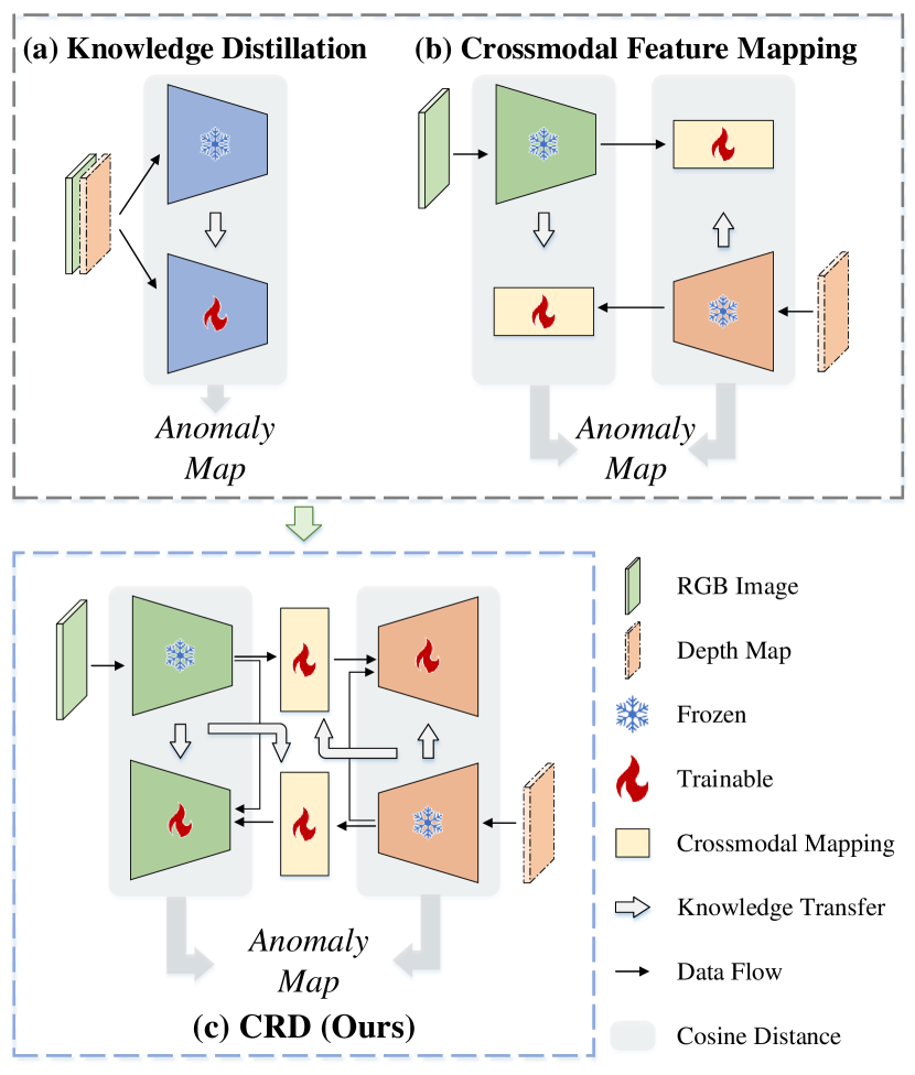
Figure 1: Comparison of our proposed Crossmodal Reverse Distillation (CRD) with other multimodal AD methods based on feature learning. The upper part contains an overview of the two previous categories of methods, and the lower part shows the overall framework of CRD.

Early unsupervised multimodal AD methods often relies on memory banks, such as BTF [18] and M3DM [28]. These methods construct large memory banks by processing and storing the multimodal features of normal samples from the training set. During inference, the extracted features are compared with the normal features in the memory bank to determine if the samples are anomalous. However, such methods inevitably require substantial storage, which becomes a bottleneck, especially when dealing with large-scale datasets.

Recent studies introduce the idea of feature learning to multimodal AD to avoid large-scale storage [24, 15, 12]. The feature learning methods typically leverage pretrained networks which is frozen during training to generate rich feature representations and transfer them to trainable networks. Since only normal samples are used during training, the trainable networks only learn the normality representation ability from the frozen networks. In other words, the abnormality representation ability is not transferred. During inference, the distances between features from the frozen and trainable networks are used to detect anomalies.

Currently, feature learning-based methods are divided into two categories as in Fig. 1: (1) Methods like AST [24] and MMRD [15] (Fig. 1 (a)) follow Knowledge Distillation, where student networks learn the multimodal feature representation ability from teacher networks on normal samples. However, these methods may smooth out abnormal features during fusion, reducing teacher’s sensitivity to anomalies and leading to false negatives, particularly when one modality is normal and the other is anomalous. (2) Crossmodal Feature Mapping [12] (Fig. 1 (b)) introduces a new paradigm, and realizes multimodal AD by mapping features across modalities to capture crossmodal relationships. But inevitably, misalignment between multimodal features results in underfitting and cause false positives in the output anomaly maps.

To address the anomaly smoothing issue in previous KD-based methods, our intuition is to expand the single-branch distillation into a multi-branch one. Each modality has its own distillation target, ensuring the sensitivity to anomalies within each modality. Additionally, to tackle the underfitting problem of Crossmodal Feature Mapping, we propose not to directly use the feature similarity from crossmodal mapping for anomaly map generation. Instead, we integrate the idea of crossmodal mapping into the multi-branch distillation, where features from another modality’s teacher network, along with the inter-modal relationship, help generate features for the student network of a given modality.

In summary, we propose a targeted extension of the widely studied KD-based AD paradigm Reverse Distillation (RD), named Crossmodal Reverse Distillation (CRD). CRD naturally combines the strengths of both feature learning paradigms. First, we design a Multi-branch Distillation (MBD) that enhances anomaly detection within each modality and refines the modality fusion process to generate more precise anomaly maps. Next, we introduce two crossmodal assistants within each modality branch. One is Crossmodal Filter (CF), which uses information from other modalities to help the student decoder generate normal features. And the other is Crossmodal Amplifier (CA), which allows a modality branch to detect anomalies from other modalities. Finally, anomaly scores of the test samples are calculated by integrating the anomaly maps of all branches. Experimental results on the representative 3D AD dataset demonstrate the effectiveness of our method in multimodal anomaly detection and localization. Our contributions are as follows:

• We propose Crossmodal Reverse Distillation based on Multi-branch Distillation for multimodal industrial anomaly detection, which effectively detects anomalies in all modalities.

• Two crossmodal assistants are introduced including Crossmodal Filter that helps the student decoder generate normal features, and Crossmodal Amplifier that amplifies the perception of anomalies from other modalities.

• Experimental results show that our proposed CRD achieves state-of-the-art performance on the multimodal industrial AD dataset.

2 Related Work

Unsupervised Anomaly Detection

Unsupervised AD has gained increasing attention in recent years. Initially, many unsupervised AD methods relied on generative models [5, 1, 34]. These models are trained on normal samples to learn the ability to reconstruct normal data. During inference, reconstruction errors are used to classify input images as normal or anomalous. Other methods introduce memory banks [23, 2, 20], comparing test samples with stored normal features to detect anomalies. Recently, there has been significant progress in the research of synthetic anomaly images [19, 30, 21], which simulate real-world scenarios to assist in unsupervised AD tasks. Additionally, knowledge distillation methods [25, 27, 24, 3, 13, 26, 16, 14, 33, 17] based on teacher-student framework have also been applied to unsupervised AD. These methods train the student network to learn the feature representations of the teacher network on normal samples, and then use the differences in feature representations between the teacher and student networks on anomalous pixels to locate anomalies. Due to the intuitive and simple nature of KD methods, KD-based AD methods have become an important focus in the field of unsupervised anomaly detection.

Multimodal Anomaly Detection

With the release of multiple 3D industrial anomaly detection datasets [7, 9, 22], unsupervised multimodal AD has gradually become a topic of research. Some methods [11], such as BTF [18] and M3DM [28], follow PatchCore [23] by leveraging memory banks for 3D AD, adding the storage of 3D features to the original PatchCore method. Other methods [10, 31, 32] rely on reconstruction networks to detect anomalies based on the reconstruction results of multimodal data. Knowledge distillation paradigms have also been explored in some methods, such as 3D-ST [4], AST [24], and MMRD [15], with the goal of having the student network mimic the multimodal features output by the teacher network. Crossmodal Feature Mapping [12] proposes a new multimodal solution, using two lightweight neural networks to perform crossmodal feature mapping and locate anomalies based on the mapping results.

3 Preliminaries

Knowledge distillation (KD) is a widely recognized and researched paradigm for unsupervised industrial image AD, typically based on a teacher-student network framework. The teacher network is usually a pretrained model, while the student network is a trainable network identical or similar to the teacher network. During training, only normal samples are used, and the teacher network’s ability to represent normal features is transferred to the student network. This process is often realized using cosine similarity. Let $F_{T}$ represent the feature output of the teacher network, and $F_{S}$ represent the feature output of the student network. The optimization loss is generally expressed as

$$\mathrm{Sim}(f_{1},f_{2})=\frac{{f_{1}}^{\mathsf{T}}f_{2}}{\|f_{1}\|\|f_{2}\|}$$ (1)

$$\mathcal{L}=\sum_{i=1}^{l}\{1-\mathrm{Sim}(F_{T}^{i},F_{S}^{i})\}$$ (2)

where $l$ represents the number of selected feature layers, typically set to 3. During inference, the multi-layer cosine distance between the teacher and student features is used, with $\mathcal{M}=\sum(1-\mathrm{Sim}(F_{T},F_{S}))$ as the anomaly map, and $\mathcal{S}=\max(\mathcal{M})$ as the anomaly score for the sample. When the input is a normal sample, the student’s features are similar to the teacher’s, thus both the values in $M$ and $S$ are low. When the input is an anomalous sample, since the student has not learned the teacher’s abnormal feature representation ability, the feature distance $M$ is large in the anomalous regions, allowing for the detection of both the presence and location of anomalies.

Reverse distillation (RD) [13] is an advanced KD-based AD method. Unlike traditional forward distillation, RD uses an encoder-decoder architecture. The teacher network is a pre-trained encoder with a WideResNet 50 [29] backbone, while the student network is a trainable decoder that generates features matching the size of the teacher’s features. RD also includes a trainable bottleneck module, OCBE, to compress features between the teacher and student. During training, the student network learns to reconstruct the teacher’s normal features using normal samples. During inference, the teacher network, with its strong feature extraction ability, captures abnormal patterns in the anomalous input and generates anomaly features. At the same time, the OCBE module compresses the teacher features, preventing abnormal information from inputting student network. As a result, even for abnormal samples, the student network generates anomaly-free features, which enables RD to detect and localize anomalies by calculating the cosine distance between the student and teacher features.

4 Crossmodal Reverse Distillation

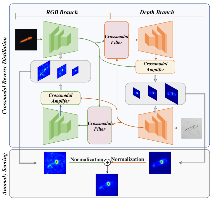
Figure 2: Pipeline of our proposed method which introduces Knowledge Distillation to the multimodal industrial AD task. Our proposed method mainly consists of two parts: (1) Cross Reverse Distillation designs multiple branches to realize Reverse Distillation for multiple modalities, (2) Anomaly Scoring aggregates anomaly maps from multiple branches to achieve multimodal anomaly detection.

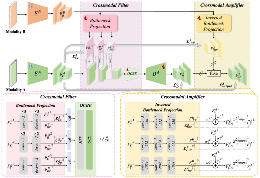
Figure 3: Information flow of the branch of Modality A, showing how Crossmodal Filter and Crossmodal Amplifier incorporate information from Modality B. Crossmodal Filter aids the student decoder in generating normal features by utilizing features from Modality B, while Crossmodal Amplifier strengthens the perception of anomalies in Modality A by amplifying anomaly signals from Modality B.

In the multimodal anomaly detection task, each input consists of multiple modalities of data. In this section, we primarily focus on RGB and Depth modalities as examples for studying multimodal anomaly detection. Therefore, each input is represented as $\mathcal{I}=\{\mathcal{I}^{RGB},\mathcal{I}^{Dep}\}$, where $\mathcal{I}^{RGB}$ and $\mathcal{I}^{Dep}$ are the RGB image and depth map respectively. The training set consists of a collection of $n$ normal samples, denoted as $\{\mathcal{I}_{train}^{1},\mathcal{I}_{train}^{2},...,\mathcal{I}_{train}^{n}\}$. The test set $\{\mathcal{I}_{test}^{1},\mathcal{I}_{test}^{2},...,\mathcal{I}_{test}^{m}\}$ contains $m$ samples, which includes both normal and anomalous samples.

4.1 Multi-branch Distillation

In multimodal industrial AD, several methods have incorporated knowledge distillation, which are broadly classified into two categories:

• Some methods add or concatenate multimodal data together at the input stage, transforming the multi-modal into a single-modal problem.

• Others employ multiple teacher networks to independently extract features from different modalities, and then merges the features as the learning target for the distillation of student network.

The core idea of these methods is to train the student network to learn the fused normal features from the teacher networks, thereby learning the normal pattern. During inference, when anomalous samples are input, the student network fails to fit the fused abnormal features from the teacher, allowing anomalies to be detected by measuring the feature distance between the student and teacher networks.

However, the effectiveness of these methods relies on a key assumption: the fused teacher features exhibit strong sensitivity to anomalies, which means they generate a significant difference between normal and anomalous regions. The issue is that in multimodal AD, it is common for one modality to be anomalous while another modality remains normal. In such cases, if the normal modality dominates the fusion, the abnormal information becomes smoothed. As a result, the fused teacher features may fail to capture the abnormal characteristics, remaining close to the normal representation. This causes the student network to fit the teacher’s features even in the anomalous regions, leading to false negatives in anomaly detection.

To resolve the problem of anomaly smoothing during modality fusion, we introduce Multi-branch Distillation (MBD) as in Fig. 2, which differs from previous KD-based multimodal AD methods with a multi-branch design. (In this section, we focus on the example case of dual-branch including RGB and depth branch, with the multi-branch scenario extending similarly.) Within MBD, each branch corresponds to a specific modality. During training, the pre-trained teacher network independently distills knowledge for each modality, eliminating the need for fusion at the input or feature exaction stages. At inference, an anomaly map is generated for each modality, and these maps are fused after normalization. By deferring the fusion of modalities to the inference stage, our method MBD allows for more precise integration of multimodal information, effectively preventing the smoothing of anomalies during feature fusion and reducing the risk of false negatives.

For the design of each branch, we draw inspiration from RD. Both the RGB and depth branches consist of four components: the frozen pre-trained teacher encoder, the trainable student decoder, and two crossmodal assistants including Crossmodal Filter and Crossmodal Amplifier (Sec. 4.2). The teacher encoders in both branches share parameters and are based on WideResNet 50 pre-trained on ImageNet. The student decoders follow the design of RD, using a structure symmetric to that of the teacher networks. Crossmodal Filter replaces the OCBE module of RD, while Crossmodal Amplifier is placed after the student decoder to optimize the output features, enabling crossmodal mapping and information fusion between modalities. The anomaly map for each branch is obtained by calculating the cosine distance between the output features of Crossmodal Amplifier and the teacher encoder.

Method/Category	Bagel	Cable Gland	Carrot	Cookie	Dowel	Foam	Peach	Potato	Rope	Tire	Average
DepthGAN [7]	53.8	37.2	58.0	60.3	43.0	53.4	64.2	60.1	44.3	57.7	53.2
DepthAE [7]	64.8	50.2	65.0	48.8	80.5	52.2	71.2	52.9	54.0	55.2	59.5
DepthVM [7]	51.3	55.1	47.7	58.1	61.7	71.6	45.0	42.1	59.8	62.3	55.5
BTF [18]	91.8	74.8	96.7	88.3	93.2	58.2	89.6	91.2	92.1	88.6	86.5
M3DM [28]	99.4	90.9	97.2	97.6	96.0	94.2	97.3	89.9	97.2	85.0	94.5
Shape-guided [11]	98.6	89.4	98.3	99.1	97.6	85.7	99.0	96.5	96.0	86.9	94.7
AST [24]	98.3	87.3	97.6	97.1	93.2	88.5	97.4	98.1	100	79.7	93.7
MMRD [15]	99.9	94.3	96.4	94.3	99.2	91.2	94.9	90.1	99.4	90.1	95.0
CFM [12]	98.8	87.5	98.4	99.2	99.7	92.4	96.4	94.9	97.9	95.0	96.0
CRD (Ours)	99.6	96.1	98.2	98.5	99.7	90.1	99.2	97.6	100	83.3	96.2

Table 1: Image-level anomaly detection results I-AUROC (%) on MVTec 3D-AD with the best in bold. We abbreviate Crossmodal Feature Mapping as CFM, the same below.

4.2 Crossmodal Assistants

To fully leverage the complementary information between modalities, we introduce crossmodal interactions within Multi-branch Distillation. To be specific, we design two crossmodal assistants serving two key purposes: (1) Crossmodal Filter (CF) helps the student network of one modality reconstruct normal features by utilizing information from another modality, even when that modality exhibits anomalies. (2) Crossmodal Amplifier (CA) allows the abnormal information from the anomalous modality to be reflected in the student features from the normal modality. With CA, the anomaly is more prominent in both branch even when one of the modalities is normal, thus prevented from being overlooked in the final detection.

Crossmodal Filter

The training objective of RD is to ensure that the student decoder generates anomaly-free features. It is achieved through the OCBE bottleneck module in vanilla RD. By further compressing the encoder features, the OCBE module effectively prevents anomaly disturbances from propagating into the student decoder, ensuring that the student decoder generates anomaly-free features even when anomaly samples are input during inference. However, in multimodal AD, relying only on the OCBE module to get the student input results in underutilization of the rich multimodal information. In particular, when one modality is anomalous and the other is normal, we believe that using the information from the normal modality aids in reconstructing the anomaly-free features of the anomalous modality. Therefore, we propose Crossmodal Filter to optimize the OCBE process by incorporating the normal information from the other modality.

Fig. 3 depicts the structure and information flow of Crossmodal Filter (discussed here with modality B assisting modality A as an example). Our proposed Crossmodal Filter module consists of two parts: Bottleneck Projection (BP) and a modified version of the OCBE module. First, BP module aligns the teacher encoder features of modality B to the teacher features of modality A, preventing interference in the decoder process of modality A during later feature fusion. Then, the aligned modality B features are concatenated with the original teacher features of modality A. The OCBE module from RD is modified to retain its feature compression capability while expanding the input feature dimensions to accommodate the fused features.

It is worth noting that to ensure the features of modality B used for assistance are normal, we mimic the concept of OCBE and design Bottleneck Projection as a two-step process of compression and restoration. First, the three encoder features ${F^{B}_{E}}^{i},i=\{1,2,3\}$ of modality B are downsampled to $8\times 8$ by convolution. Then, these features are upsampled back to their original size using deconvolution to obtain ${F^{B}_{BP}}^{i},i=\{1,2,3\}$. During training, we minimize the distance between $F^{B}_{BP}$ and the teacher encoder features of modality A $F^{A}_{E}$, mapping modality B’s features into modality A’s feature space. During inference, the feature compact process of BP helps reduce the interference of anomalies in modality B, ensuring that normal information from modality B is effectively transferred to the modality A’s branch.

Crossmodal Amplifier

When only one modality has anomalies, multimodal fusion may lead to anomaly smoothing, resulting in false negatives, as discussed in Sec. 4.1. We address this issue with Multi-branch Distillation. However, fusion of the anomaly maps still cause the anomaly values to become less noticeable after summation. Our idea is that multimodal information interaction helps resolve this issue. Specifically, when modality A is normal and modality B is anomalous, if the anomaly information from modality B is incorporated into modality A’s branch, the anomaly map generated by modality A is also able to show the anomalies in modality B. This allows the anomaly in modality B to be emphasized in modality A’s branch, thus preventing the anomaly smoothing issue during anomaly map fusion.

As illustrated in Fig. 3, we design Crossmodal Amplifier. First, Inverted Bottleneck Projection (IBP) is designed to map modality B’s features to modality A’s feature space, yielding ${F^{B}_{IBP}}^{i},i=\{1,2,3\}$. Then, the mapped features are then dynamically fused with the features ${F^{A}_{D}}^{i},i=\{1,2,3\}$ which are reconstructed by the student decoder in modality A’s branch, to obtain ${F^{A}_{CA}}^{i},i=\{1,2,3\}$ by

$${F^{A}_{CA}}^{i}=\frac{\exp({w_{1}^{A}}^{i})*{F^{A}_{D}}^{i}+\exp({w_{2}^{A}}^{i})*{F^{B}_{IBP}}^{i}}{\exp({w_{1}^{A}}^{i})+\exp({w_{2}^{A}}^{i})}$$ (3)

where $w_{1}^{A}$ and $w_{2}^{A}$ are trainable parameters, initially set to 1.0 during training.

Inverted Bottleneck Projection only learns to map modality B’s normal features to modality A’s feature space during training. It means that IBP is not able to make the correct feature mapping when modality B has anomalies in the test sample. Therefore, the fused feature ${F^{A}_{CA}}$ includes modality B’s anomalous information, which leads to a larger distance between the teacher encoder’s features $F^{A}_{E}$ and ${F^{A}_{CA}}$, allowing the anomaly in modality B to be detected in modality A’s branch.

In contrast to Bottleneck Projection in CF, the proposed Inverted Bottleneck Projection first expands the dimensions of features and then compresses them to the original sizes. We believe that this process makes the IBP module more sensitive to distinct features, thereby better preserving the influence of anomaly information in the modality during feature mapping.

4.3 Training Objectives

The overall optimization objective of our method is composed of three main components. Firstly, similar to the approach in RD, we optimize the features output by the student decoder using cosine similarity as

$$\mathcal{L}^{RGB/Dep}_{D}=\sum_{i=1}^{3}\{1-\mathrm{Sim}({F_{E}^{RGB/Dep}}^{i},{F_{D}^{RGB/Dep}}^{i})\}$$ (4)

where $\mathcal{L}^{RGB}_{D}$ and $\mathcal{L}^{Dep}_{D}$ are the losses corresponding to RGB and depth branches respectively.

Secondly, to ensure the effectiveness of Crossmodal Filter, it is crucial to align the mapping features $F_{BP}^{Dep/RGB}$ within these filters to the encoder features. The training losses of RGB and Depth branches are calculated as:

$$\mathcal{L}^{RGB/Dep}_{CF}=\sum_{i=1}^{3}\{1-\mathrm{Sim}({F_{E}^{RGB/Dep}}^{i},{F_{BP}^{Dep/RGB}}^{i})\}$$ (5)

Finally, Crossmodal Amplifier needs to be optimized,, which includes the optimization of feature mapping and feature fusion parameters $\{w_{1},w_{2}\}$. The total loss function is

$$\mathcal{L}^{RGB/Dep}_{CA}=\mathcal{L}^{RGB/Dep}_{IBP}+\mathcal{L}^{RGB/Dep}_{output}$$ (6)

$$\mathcal{L}^{RGB/Dep}_{IBP}=\sum_{i=1}^{3}\{1-\mathrm{Sim}({F_{E}^{RGB/Dep}}^{i},{F_{IBP}^{Dep/RGB}}^{i})\}$$ (7)

$$\mathcal{L}^{RGB/Dep}_{output}=\sum_{i=1}^{3}\{1-\mathrm{Sim}({F_{E}^{RGB/Dep}}^{i},{F_{CA}^{RGB/Dep}}^{i})\}$$ (8)

The overall loss $\mathcal{L_{CRD}}$ is expressed as

$$\begin{split}\mathcal{L}_{CRD}&=(\mathcal{L}^{RGB}_{D}+\mathcal{L}^{RGB}_{CF}+\mathcal{L}^{RGB}_{CA})\\ &+(\mathcal{L}^{Dep}_{D}+\mathcal{L}^{Dep}_{CF}+\mathcal{L}^{Dep}_{CA})\end{split}$$ (9)

Since each part has independent optimizers and inputs, the hyper-parameters are set to 1.

4.4 Anomaly Scoring

Following previous KD-based methods, we generate the anomaly map for each branch using cosine distance as

$$\mathcal{M}^{RGB/Dep}=\sum_{1}^{3}(1-\mathrm{Sim}({F_{E}^{RGB/Dep}}^{i},{F_{CA}^{RGB/Dep}}^{i}))$$ (10)

For the fusion of anomaly maps of two branches, we refer to the method in [8]:

• First, we calculate the means and standard deviations of the values in the anomaly maps using all normal samples from the validation set, denoted as $\mu^{RGB/Dep}$ and $\sigma^{RGB/Dep}$, respectively.

• Then, during inference, we normalize the anomaly maps for both branches as

  $$\mathcal{M}^{RGB/Dep}_{norm}=\frac{\mathcal{M}^{RGB/Dep}-\mu^{RGB/Dep}}{\sigma^{RGB/Dep}}$$ (11)

• Finally, we rescale the maps to the same scale and sum the anomaly maps from both branches to obtain the final anomaly map as $\mathcal{M}=\mathcal{M}^{RGB}_{norm}+\mathcal{M}^{Dep}_{norm}$.

And we simply choose $\mathcal{S}=\max(\mathcal{M})$ as the anomaly score.

Method/Category	Bagel	Cable Gland	Carrot	Cookie	Dowel	Foam	Peach	Potato	Rope	Tire	Average
DepthGAN [7]	42.1	42.2	77.8	69.6	49.4	25.2	28.5	36.2	40.2	63.1	47.4
DepthAE [7]	43.2	15.8	80.8	49.1	84.1	40.6	26.2	21.6	71.6	47.8	48.1
DepthVM [7]	38.8	32.1	19.4	57.0	40.8	28.2	24.4	34.9	26.8	33.1	33.5
BTF [18]	97.6	96.9	97.9	97.3	93.3	88.8	97.5	98.1	95.0	97.1	95.9
M3DM [28]	97.0	97.1	97.9	95.0	94.1	93.2	97.7	97.1	97.1	97.5	96.4
Shape-guided [11]	98.1	97.3	98.2	97.1	96.2	97.8	98.1	98.3	97.4	97.5	97.6
AST [24]	97.0	94.7	98.1	93.9	91.3	90.6	97.9	98.2	88.9	94.0	94.4
MMRD [15]	98.6	99.0	99.1	95.1	99.0	90.1	99.0	99.0	98.7	98.2	97.6
CFM [12]	98.0	96.6	98.2	94.7	95.9	96.7	98.2	98.3	97.6	98.2	97.2
CRD (Ours)	97.7	98.1	99.1	98.2	98.7	91.0	99.4	99.5	98.2	97.4	97.7

Table 2: Pixel-level anomaly localization results PRO (%) on MVTec 3D-AD with the best in bold.

5 Experiments

5.1 Experimental Settings

Dataset

We conduct experiments on MVTec 3D-AD [7] dataset which is a 3D industrial anomaly detection dataset that includes 10 categories of industrial objects. The training set contains a total of 2,656 normal samples, each consisting of an RGB image and corresponding 3D scan information. The test set includes 1,197 samples, comprising both 948 anomalous samples and 249 normal samples, and provides pixel-level annotations for anomaly detection and localization evaluation. Besides, a validation set is provided by MVTec 3D-AD, containing 294 normal samples.

Evaluation Metrics

The evaluation metrics for anomaly detection include image-level area under the receiver operating characteristic curve (I-AUROC) and average precision (I-AP). For anomaly localization, pixel-level AUROC (P-AUROC) and AP (P-AP) are used. We also employ the per-region overlap (PRO) metric calculated according to the official code [7] for anomaly localization, which treats anomaly regions of different size equally.

Implementation Details

During both training and inference, only the depth information from the 3D data is used. All RGB images and depth maps are scaled to $256\times 256$. The training is performed on a single Nvidia GTX 3090 GPU, and a separate detection model is trained for each category. The network backbone is WideResNet 50. The batch size is 16, and the training lasts for 200 epochs. Each branch is optimized using a separate Adam optimizer with a learning rate of 0.005. In inference, the anomaly maps of both branches are smoothed using a Gaussian filter with $\sigma=4$.

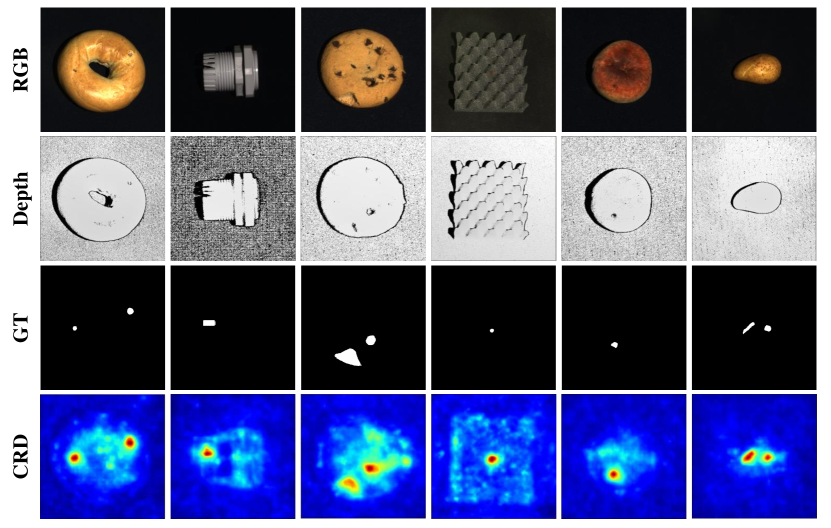
Figure 4: Qualitative results on MVTec-3D AD. From top to bottom: the input images, the corresponding depth maps, the ground truth masks, the output anomaly maps of our proposed CRD.

5.2 Results on MVTec-3D AD

Tab. 1 and Tab. 2 show the quantitative image-level anomaly detection results and pixel-level anomaly localization results on the MVTec 3D-AD dataset. We compare our method, CRD, with several state-of-the-art 3D anomaly detection methods. CRD consistently outperforms all other methods in both I-AUROC and PRO metrics, achieving an average I-AUROC of 96.2% and an average PRO of 97.7%. Notably, CRD demonstrates superior performance in detecting and localizing anomalies across a wide range of categories, including some challenging categories such as Cookie and Peach.

A subset of qualitative results on MVTec-3D AD is provided in Fig. 4, showing that our proposed CRD is able to accurately localize the anomaly regions. For further details on P-AUROC results and more qualitative results please refer to the Supplementary Materials.

5.3 Ablation Studies

Study on Multi-branch Distillation

Branch	I-AUROC	P-AUROC	P-PRO	I-AP	P-AP
RGB	86.8	98.9	95.4	95.8	37.7
RGB+Crossmodal	88.9	99.0	95.8	96.5	39.4
Depth	87.1	96.2	88.8	95.2	33.7
Depth+Crossmodal	87.3	97.1	90.1	95.7	34.1
RGB+Depth	93.9	99.3	97.4	98	45.2
RGB+Depth+Crossmodal	96.2	99.4	97.7	98.8	45.5

Table 3: Ablation study results (%) of Multi-branch Distillation on MVTec 3D-AD.

We conduct an ablation study in Tab. 3, which demonstrates that the multi-branch setup, combining both RGB and Depth modalities, significantly outperforms individual modality branches. The I-AUROC metric of 93.9% for using both branches is higher than 86.8% for RGB branch only and 87.1% for depth branch only, highlighting the complementary benefits of modality fusion.

Study on Crossmodal Assistants

CF	CA	I-AUROC	P-AUROC	P-PRO	I-AP	P-AP
-	-	93.9	99.3	97.4	98	45.2
✓	-	94.2	99.3	97.5	98.2	45.8
-	✓	95.6	99.4	97.7	98.6	45.5
✓	✓	96.2	99.4	97.7	98.8	45.5

Table 4: Ablation study results (%) of Crossmodal Assistants on MVTec 3D-AD.

We perform an ablation study to evaluate the impact of Crossmodal Filter and Crossmodal Amplifier on anomaly detection performance, as shown in Tab. 4. The results reveal that both CF and CA contribute to improved performance, with the combination of both achieving the best results. Specifically, adding CF to the baseline improves I-AUROC from 93.9% to 94.2%, and incorporating CA also boosts the performance, achieving an I-AUROC of 95.6%. The highest performance is achieved when both CF and CA are used together, resulting in an I-AUROC of 96.2%.

Study on Bottlneck Projection in Crossmodal Filter

Downsampling Size	I-AUROC	P-AUROC	P-PRO	I-AP	P-AP
Identity	93.9	99.3	97.4	98.0	45.8
$16\times 16$	93.6	99.3	97.4	97.9	45.2
$8\times 8$	94.2	99.3	97.5	98.2	45.8
$4\times 4$	93.8	99.3	97.4	98.0	45.3

Table 5: Ablation study results (%) of different downsampling sizes in Bottlneck Projection on MVTec 3D-AD.

We investigate the effect of different downsampling sizes on the performance of the Crossmodal Filter, as shown in Tab. 5. When Bottleneck Projection reduces the feature size to $8\times 8$, the model achieves the best performance across multiple metrics. It is observed that excessively large downsampling size (e.g., $4\times 4$) leads to information loss, while too small downsampling size (e.g., $16\times 16$) makes it difficult to filter out abnormal interference effectively. Therefore, we conclude that selecting an appropriate downsampling size is crucial for maintaining a balance between information preservation and interference removal.

Study on Inverted Bottlneck Projection in Crossmodal Amplifier

Channel Expansion	I-AUROC	P-AUROC	P-PRO	I-AP	P-AP
Identity	95.7	99.3	97.7	98.7	45.1
$2\times$	95.6	99.4	97.7	98.6	45.5
$4\times$	95.7	99.4	97.7	98.6	45.0

Table 6: Ablation study results (%) of different channel expansion sizes in Inverted Bottlneck Projection on MVTec 3D-AD.

As recorded in Tab. 6, we analyze the impact of different channel expansion sizes on the performance of the Crossmodal Amplifier. The results demonstrate that a 2 times channel expansion strikes the best balance between detection performance and computational efficiency. This configuration achieves a high PRO of 97.7% and a P-AP of 45.5%, while maintaining relatively low computational overhead compared to the 4 times expansion.

Study on Anomaly Scoring

Aggregation	I-AUROC	P-AUROC	P-PRO	I-AP	P-AP
$\mathcal{M}^{RGB}_{norm}+\mathcal{M}^{Dep}_{norm}$	96.2	99.4	97.7	98.8	45.5
$\mathcal{M}^{RGB}+\mathcal{M}^{Dep}$	95.6	99.1	97.6	98.6	44.4
$(\mathcal{M}^{RGB}/3)\cdot(\mathcal{M}^{Dep}/3)$ [12]	94.3	99.3	97.2	98.2	43.5

Table 7: Ablation study results (%) of anomaly map aggregation strategy on MVTec 3D-AD.

Tab. 7 demonstrates that normalizing the anomaly maps from each modality before summing them performs better than directly adding or multiplying the maps. Normalization ensures the anomaly maps from different modalities are on the same scale, making fusion more effective. As a result, normalizing before aggregation improves performance across all metrics.

6 Conclusion

In this paper, Crossmodal Reverse Distillation is proposed, which offers a novel solution based on Knowledge Distillation for unsupervised multimodal industrial AD task by fully utilizing the information from all modalities. CRD uses a multi-branch design to independently process each modality, enabling more accurate anomaly detection in each branch. Additionally, two crossmodal assistants are introduced: Crossmodal Filter helps the student decoder generate normal features, and Crossmodal Amplifier aims to amplify anomalies of one modality to branches of other modalities. Experimental results on MVTec 3D-AD show that CRD achieves SOTA performance in both anomaly detection and localization.

Supplementary Material

Appendix A Motivation

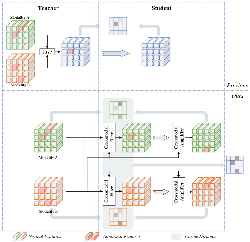
Figure 5: Feature diagrams in the anomaly detection process based on Knowledge Distillation. The upper part illustrates previous methods (using RD framework as an example), while the lower part represents the feature transformation in our proposed method CRD. Green and orange indicate two modalities, while blue represents the fused results. In the resulting anomaly maps, darker gray regions indicate higher anomaly scores.

In Sec. 4.1, In Sec 4.1, we introduce the detection approach of previous unsupervised multimodal anomaly detection methods based on Knowledge Distillation. These methods detect and localize anomalies by analyzing the differences between the fused multimodal teacher features and student features. We also identify a key issue in these methods: the anomaly smoothing problem. When features from a normal modality dominate the fusion, abnormal information may be smoothed out, resulting in fused teacher features that fail to effectively reflect the anomalies.

This section provides an illustrative diagram to further explain this problem. In Fig. 5, the upper part outlines the feature transformation process of previous KD-based methods, while the lower part illustrates the feature transformation process in our proposed method. Unlike prior methods, which may miss anomalies when one modality is normal and the other is abnormal, our method ensures sensitivity to anomalies in each modality through dual-branch processing. Additionally, the proposed crossmodal assistants facilitate interaction between modalities, enabling more precise anomaly detection and localization.

Appendix B P-AUROC on on MVTec 3D-AD

Method/Category	Bagel	Cable Gland	Carrot	Cookie	Dowel	Foam	Peach	Potato	Rope	Tire	Average
BTF [18]	99.6	99.2	99.7	99.4	98.1	97.4	99.6	99.8	99.4	99.5	99.2
M3DM [28]	99.5	99.3	99.7	98.5	98.5	98.4	99.6	99.4	99.7	99.6	99.2
AST [24]	-	-	-	-	-	-	-	-	-	-	97.6
MMRD [15]	-	-	-	-	-	-	-	-	-	-	99.2
CFM [12]	99.7	99.2	99.9	97.2	98.7	99.3	99.8	99.9	99.8	99.8	99.3
CRD (Ours)	99.3	99.3	99.8	99.3	99.7	97.4	99.8	99.9	99.7	99.5	99.4

Table 8: Pixel-level anomaly localization results P-AUROC (%) on MVTec 3D-AD with the best in bold.

This section compares our method with other mainstream multimodal AD methods using the P-AUROC metric, including memory bank-based methods BTF [18] and M3DM [28], KD-based methods AST [24] and MMRD [15], and Crossmodal Feature Mapping CFM [12]. As shown in Tab. 8, our method achieves SOTA performance, reaching 99.4% on the P-AUROC metric. Notably, for certain categories like Dowel, our CRD significantly outperforms previous methods. In most other categories, it consistently maintains competitive or near-optimal performance.

Appendix C Additional Results of Ablation Studies

In the main text, we present five aspects of ablation studies:

1. Study on Multi-branch Distillation demonstrates that combining the distillation results from multiple branches of different modalities achieves better performance, highlighting the importance of multiple branches. (Tab. 9)

2. Study on Crossmodal Assistants shows that incorporating crossmodal assistants into Multi-branch Distillation based on Reverse Distillation significantly improves anomaly detection, proving their effectiveness. (Tab. 10)

3. Study on Bottleneck Projection in Crossmodal Filter explores the impact of downsampling sizes in the Bottleneck Projection module of Crossmodal Filter, concluding that a size of $8\times 8$ yields optimal results. (Tab. 11)

4. Study on Inverted Bottleneck Projection in Crossmodal Amplifier investigates the effect of channel expansion in the Inverted Bottleneck Projection module of Crossmodal Amplifier, finding that a $2\times$ expansion achieves the best performance. (Tab. 12)

5. Study on Anomaly Scoring examines different methods for fusing anomaly maps from multiple branches, confirming that our selected approach delivers the best results. (Tab. 13)

In the main text, we provide average results across all categories for comparison. Here, we present detailed results for each category, as shown in Tab. 9, Tab. 10, Tab. 11, Tab. 12, and Tab. 13.

Metrics	Branch	Bagel	Cable Gland	Carrot	Cookie	Dowel	Foam	Peach	Potato	Rope	Tire	Average
I-AUROC	RGB	97.8	94.0	93.9	58.6	98.5	85.3	91.8	62.1	99.2	86.3	86.8
	RGB+Crossmodal	98.7	97.6	94.2	65.7	98.4	88.1	91.6	66.5	97.9	90.3	88.9
	Depth	99.1	63.8	97.8	99.5	85.3	73.5	99.4	98.8	98.3	55.2	87.1
	Depth+Crossmodal	98.3	67.6	98.1	99.1	86.1	76.6	99.2	99.4	98.1	50.5	87.3
	RGB+Depth	99.7	89.8	97.8	97.1	99.9	81.3	99.4	96.8	99.9	77.2	93.9
	RGB+Depth+Crossmodal	99.6	96.1	98.2	98.5	99.7	90.1	99.2	97.6	100	83.3	96.2
P-AUROC	RGB	99.3	99.5	99.5	98.0	99.5	96.1	99.4	99.4	99.4	99.1	98.9
	RGB+Crossmodal	99.4	99.6	99.5	98.5	99.5	95.9	99.4	99.4	99.4	99.2	99.0
	Depth	99.0	94.0	99.8	99.0	98.7	78.5	99.8	99.9	99.5	93.7	96.2
	Depth+Crossmodal	98.9	93.8	99.8	98.9	99.2	84.8	99.8	99.9	99.5	95.9	97.1
	RGB+Depth	99.4	99.3	99.7	99.4	99.6	97.2	99.8	99.9	99.6	99.1	99.3
	RGB+Depth+Crossmodal	99.3	99.3	99.8	99.3	99.7	97.4	99.8	99.9	99.7	99.5	99.4
PRO	RGB	97.2	98.6	98.3	89.4	97.3	87.3	97.8	97.6	95.5	95.3	95.4
	RGB+Crossmodal	97.8	98.9	98.2	92.1	97.3	86.6	97.7	97.7	95.5	95.7	95.8
	Depth	97.0	81.3	99.1	97.6	95.4	47.5	99.3	99.6	96.2	75.3	88.8
	Depth+Crossmodal	96.7	80.0	99.1	97.5	96.9	51.8	99.4	99.6	96.8	82.9	90.1
	RGB+Depth	98.2	98.0	99.0	98.2	98.4	90.2	99.3	99.5	98.0	95.4	97.4
	RGB+Depth+Crossmodal	97.7	98.1	99.1	98.2	98.7	91.0	99.4	99.5	98.2	97.4	97.7
I-AP	RGB	99.4	98.5	98.6	86.9	99.7	96.0	97.8	86.0	99.7	95.3	95.8
	RGB+Crossmodal	99.7	99.4	98.7	88.3	99.7	97.0	97.7	88.7	99.2	97.0	96.5
	Depth	99.8	88.9	99.5	99.9	95.7	89.8	99.8	99.7	99.3	79.4	95.2
	Depth+Crossmodal	99.6	91.2	99.6	99.8	95.7	92.9	99.8	99.9	99.2	79.0	95.7
	RGB+Depth	99.9	97.3	99.5	99.2	100	93.9	99.9	98.9	99.9	91.3	98.0
	RGB+Depth+Crossmodal	99.9	99.1	99.6	99.6	99.9	97.1	99.8	99.3	100	93.7	98.8
P-AP	RGB	49.2	42.9	31.8	47.6	43.6	23.0	37.8	17.9	52.1	31.4	37.7
	RGB+Crossmodal	52.2	44.8	30.8	52.3	49.9	23.0	35.2	21.0	50.5	34.0	39.4
	Depth	23.9	8.4	45.7	56.4	21.5	8.9	59.7	59.7	49.2	3.3	33.7
	Depth+Crossmodal	20.7	2.6	47.3	54.7	26.8	9.9	64.7	58.5	51.5	4.1	34.1
	RGB+Depth	42.3	38.2	41.6	71.4	40.7	26.9	58.8	56.7	53.5	22.2	45.2
	RGB+Depth+Crossmodal	27.9	36.7	42.8	70.1	50.1	29.4	62.9	57.4	54.8	22.7	45.5

Table 9: Ablation study results (%) of Multi-branch Distillation on MVTec 3D-AD.

Metrics	CF	CA	Bagel	Cable Gland	Carrot	Cookie	Dowel	Foam	Peach	Potato	Rope	Tire	Average
I-AUROC	-	-	99.7	89.8	97.8	97.1	99.9	81.3	99.4	96.8	99.9	77.2	93.9
	✓	-	99.5	91.3	97.7	95.2	99.7	84.4	99.2	96.6	99.8	78.2	94.2
	-	✓	99.7	93.5	98.5	98.1	99.7	88.9	99.5	97.3	100	80.4	95.6
	✓	✓	99.6	96.1	98.2	98.5	99.7	90.1	99.2	97.6	100	83.3	96.2
P-AUROC	-	-	99.4	99.3	99.7	99.4	99.6	97.2	99.8	99.9	99.6	99.1	99.3
	✓	-	99.4	99.3	99.7	99.3	99.7	97.2	99.8	99.9	99.6	99.2	99.3
	-	✓	99.3	99.3	99.7	99.3	99.7	97.5	99.8	99.9	99.7	99.4	99.4
	✓	✓	99.3	99.3	99.8	99.3	99.7	97.4	99.8	99.9	99.7	99.5	99.4
PRO	-	-	98.2	98.0	99.0	98.2	98.4	90.2	99.3	99.5	98.0	95.4	97.4
	✓	-	98.2	98.0	99.0	98.0	98.4	90.5	99.3	99.5	97.9	95.8	97.5
	-	✓	97.8	98.3	99.1	98.2	98.6	91.4	99.3	99.5	98.2	96.7	97.7
	✓	✓	97.7	98.1	99.1	98.2	98.7	91.0	99.4	99.5	98.2	97.4	97.7
I-AP	-	-	99.9	97.3	99.5	99.2	100	93.9	99.9	98.9	99.9	91.3	98.0
	✓	-	99.9	97.8	99.5	98.7	99.9	95.5	99.8	99.0	99.9	91.9	98.2
	-	✓	99.9	98.5	99.7	99.5	99.9	96.9	99.9	99.2	100	92.6	98.6
	✓	✓	99.9	99.1	99.6	99.6	99.9	97.1	99.8	99.3	100	93.7	98.8
P-AP	-	-	42.3	38.2	41.6	71.4	40.7	26.9	58.8	56.7	53.5	22.2	45.2
	✓	-	47.4	37.1	41.4	69.6	41.4	27.8	61.2	57.9	52.2	22.4	45.8
	-	✓	30.5	39.4	42.6	69.6	48.8	29.1	61.3	57.4	55.0	20.9	45.5
	✓	✓	27.9	36.7	42.8	70.1	50.1	29.4	62.9	57.4	54.8	22.7	45.5

Table 10: Ablation study results (%) of Crossmodal Assistants on MVTec 3D-AD.

Metrics	Downsampling Size	Bagel	Cable Gland	Carrot	Cookie	Dowel	Foam	Peach	Potato	Rope	Tire	Average
I-AUROC	Identity	99.6	88.8	97.9	95.6	99.7	84.6	98.8	96.8	99.8	77.1	93.9
	$16\times 16$	99.7	88.1	97.6	96.9	100	81.6	99.2	96.7	99.8	76.7	93.6
	$8\times 8$	99.5	91.3	97.7	95.2	99.7	84.4	99.2	96.6	99.8	78.2	94.2
	$4\times 4$	99.7	89.5	98.1	95.6	99.9	81.6	98.8	96.8	99.8	77.5	93.8
P-AUROC	Identity	99.4	99.3	99.7	99.3	99.7	97.2	99.8	99.9	99.6	99.1	99.3
	$16\times 16$	99.4	99.3	99.7	99.3	99.7	97.3	99.8	99.9	99.6	99.1	99.3
	$8\times 8$	99.4	99.3	99.7	99.3	99.7	97.2	99.8	99.9	99.6	99.2	99.3
	$4\times 4$	99.4	99.3	99.7	99.3	99.6	97.0	99.8	99.9	99.6	99.1	99.3
PRO	Identity	98.2	98.0	99.0	98.1	98.4	90.2	99.3	99.5	98.0	95.6	97.4
	$16\times 16$	98.1	98.0	99.0	98.1	98.4	90.6	99.2	99.5	98.0	95.5	97.4
	$8\times 8$	98.2	98.0	99.0	98.0	98.4	90.5	99.3	99.5	97.9	95.8	97.5
	$4\times 4$	98.1	98.1	99.0	98.0	98.4	89.8	99.2	99.5	98.0	95.7	97.4
I-AP	Identity	99.9	96.9	99.5	98.8	99.9	95.5	99.7	99.0	99.9	91.3	98.0
	$16\times 16$	99.9	96.7	99.5	99.2	100	93.9	99.8	98.9	99.9	90.9	97.9
	$8\times 8$	99.9	97.8	99.5	98.7	99.9	95.5	99.8	99.0	99.9	91.9	98.2
	$4\times 4$	99.9	97.3	99.6	98.8	100	93.8	99.7	98.9	99.9	91.8	98.0
P-AP	Identity	45.7	37.5	41.2	69.3	40.6	27.8	62.2	57.5	52.8	23.2	45.8
	$16\times 16$	42.7	37.1	41.4	70.2	41.3	27.3	59.6	56.8	52.9	22.3	45.2
	$8\times 8$	47.4	37.1	41.4	69.6	41.4	27.8	61.2	57.9	52.2	22.4	45.8
	$4\times 4$	44.4	38.0	41.6	70.1	40.6	26.4	59.3	56.1	54.0	22.8	45.3

Table 11: Ablation study results (%) of different downsampling sizes in Bottlneck Projection on MVTec 3D-AD.

Metrics	Channel Expansion	Bagel	Cable Gland	Carrot	Cookie	Dowel	Foam	Peach	Potato	Rope	Tire	Average
I-AUROC	Identity	99.6	95.2	98.3	98.0	99.7	87.4	99.2	97.6	100	81.9	95.7
	$2\times$	99.7	93.5	98.5	98.1	99.7	88.9	99.5	97.3	100	80.4	95.6
	$4\times$	99.5	94.7	98.0	98.6	99.7	88.8	99.2	97.5	100	80.8	95.7
P-AUROC	Identity	99.3	99.4	99.7	99.3	99.7	97.4	99.8	99.5	99.7	99.4	99.3
	$2\times$	99.3	99.3	99.7	99.3	99.7	97.5	99.8	99.9	99.7	99.4	99.4
	$4\times$	99.3	99.3	99.7	99.3	99.7	97.6	99.8	99.9	99.7	99.4	99.4
PRO	Identity	97.6	98.3	99.1	98.2	98.6	90.9	99.3	99.5	98.2	97.0	97.7
	$2\times$	97.8	98.3	99.1	98.2	98.6	91.4	99.3	99.5	98.2	96.7	97.7
	$4\times$	97.7	98.2	99.1	98.2	98.6	91.6	99.3	99.5	98.2	96.8	97.7
I-AP	Identity	99.9	98.9	99.6	99.5	99.9	96.5	99.8	99.3	100	93.2	98.7
	$2\times$	99.9	98.5	99.7	99.5	99.9	96.9	99.9	99.2	100	92.6	98.6
	$4\times$	99.9	98.7	99.5	99.6	99.9	96.9	99.8	99.3	100	92.8	98.6
P-AP	Identity	27.9	39.9	42.1	67.6	49.8	28.4	62.0	57.0	55.4	21.3	45.1
	$2\times$	30.5	39.4	42.6	69.6	48.8	29.1	61.3	57.4	55.0	20.9	45.5
	$4\times$	29.0	38.4	42.4	68.1	48.8	29.1	60.9	57.3	55.7	20.4	45.0

Table 12: Ablation study results (%) of different channel expansion sizes in Inverted Bottlneck Projection on MVTec 3D-AD.

Metrics	Aggregation	Bagel	Cable Gland	Carrot	Cookie	Dowel	Foam	Peach	Potato	Rope	Tire	Average
I-AUROC	$\mathcal{M}^{RGB}_{norm}+\mathcal{M}^{Dep}_{norm}$	99.6	96.1	98.2	98.5	99.7	90.1	99.2	97.6	100	83.3	96.2
	$\mathcal{M}^{RGB}+\mathcal{M}^{Dep}$	99.6	92.9	98.3	98.3	99.3	90.3	98.9	96.7	100	81.6	95.6
	$(\mathcal{M}^{RGB}/3)\cdot(\mathcal{M}^{Dep}/3)$ [12]	99.6	89.8	98.4	98.9	99.8	82.4	99.0	96.4	100	78.8	94.3
P-AUROC	$\mathcal{M}^{RGB}_{norm}+\mathcal{M}^{Dep}_{norm}$	99.3	99.3	99.8	99.3	99.7	97.4	99.8	99.9	99.7	99.5	99.4
	$\mathcal{M}^{RGB}+\mathcal{M}^{Dep}$	99.4	96.8	99.8	99.3	99.7	97.4	99.8	99.9	99.7	99.5	99.1
	$(\mathcal{M}^{RGB}/3)\cdot(\mathcal{M}^{Dep}/3)$ [12]	99.4	98.9	99.8	99.3	99.7	97.0	99.8	99.9	99.7	99.5	99.3
PRO	$\mathcal{M}^{RGB}_{norm}+\mathcal{M}^{Dep}_{norm}$	97.7	98.1	99.1	98.2	98.7	91.0	99.4	99.5	98.2	97.4	97.7
	$\mathcal{M}^{RGB}+\mathcal{M}^{Dep}$	97.8	96.8	99.1	98.2	98.7	91.1	99.3	99.5	98.2	97.2	97.6
	$(\mathcal{M}^{RGB}/3)\cdot(\mathcal{M}^{Dep}/3)$ [12]	98.0	96.9	99.1	98.2	98.6	88.9	99.4	99.5	98.1	95.7	97.2
I-AP	$\mathcal{M}^{RGB}_{norm}+\mathcal{M}^{Dep}_{norm}$	99.9	99.1	99.6	99.6	99.9	97.1	99.8	99.3	100	93.7	98.8
	$\mathcal{M}^{RGB}+\mathcal{M}^{Dep}$	99.9	98.2	99.6	99.6	99.8	97.2	99.7	99.0	100	92.7	98.6
	$(\mathcal{M}^{RGB}/3)\cdot(\mathcal{M}^{Dep}/3)$ [12]	99.9	97.3	99.7	99.7	100	94.1	99.6	98.9	100	92.5	98.2
P-AP	$\mathcal{M}^{RGB}_{norm}+\mathcal{M}^{Dep}_{norm}$	27.9	36.7	42.8	70.1	50.1	29.4	62.9	57.4	54.8	22.7	45.5
	$\mathcal{M}^{RGB}+\mathcal{M}^{Dep}$	31.6	27.0	43.9	70.4	48.8	29.6	60.3	55.9	55.3	21.2	44.4
	$(\mathcal{M}^{RGB}/3)\cdot(\mathcal{M}^{Dep}/3)$ [12]	37.8	28.6	42.5	72.1	45.7	17.6	60.5	54.3	54.2	21.4	43.5

Table 13: Ablation study results (%) of anomaly map aggregation strategy on MVTec 3D-AD.

Appendix D Additional Qualitative Results

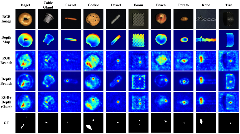
Figure 6: Qualitative results on MVTec-3D AD. From top to bottom: the input images, the corresponding depth maps, the output anomaly maps of RGB branch, the output anomaly maps of depth branch, the output anomaly maps of CRD, and the ground truth masks.

This section first provides visualizations of the anomaly maps generated by each branch and the fused results, as shown in Fig. 6. The visualizations reveal two key findings: (1) In the depth branch, the significant variation in depth values along edges introduces abundant edge information, making it challenging for student features to fit teacher features at edge regions, leading to false positives. But this issue is less pronounced in the RGB branch. (2) Some anomalies are modality-specific. For instance, discoloration is only detectable in RGB images, while the absence of chocolate on cookies is only evident in depth maps. Consequently, anomaly maps from individual branches may fail to fully capture all anomalies within a sample. However, the fused results effectively achieve comprehensive anomaly localization.

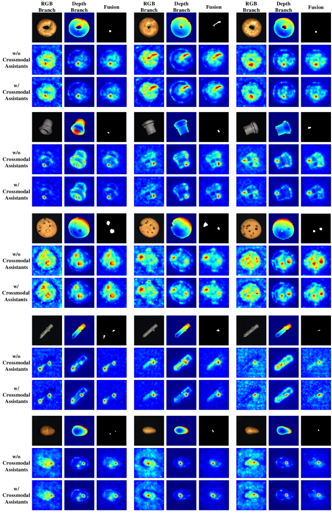
Figure 7: Qualitative results on MVTec-3D AD. From top to bottom: the examples of Bagel, Cable Cland, Cookie, Dowel, and Potato.

We also provide visualizations of anomaly maps before and after incorporating the crossmodal assistants, as in Fig. 7. Without the crossmodal assistants, anomalies that are less prominent in a specific modality goes undetected in the corresponding branch. However, after introducing the crossmodal assistants, this issue is significantly mitigated, resulting in a noticeable reduction in the anomaly miss rate across all modality branches.

Appendix E Results on Eyecandies

E.1 Eyecandies Dataset

The Eyecandies dataset is a synthetic industrial dataset featuring 10 categories of candy samples in an industrial conveyor scenario. Each sample includes RGB images, depth map, and surface normal map. The training set contains 10k samples, with 1k samples per category. The validation and test sets comprise 1k validation samples and 4k test samples, respectively. In our experiments, we select normal maps as the 3D modality and chose images under consistent lighting conditions as the 2D modality for all samples.

E.2 Quantitative result

This section presents the quantitative results of anomaly detection and localization on Eyecandies in Tab. 14. The primary comparison methods include RGB-D [9] and RGB-cD-n [9], proposed alongside the dataset, memory bank-based methods such as BTF [18] and M3DM [28], KD-based methods like AST [24] and MMRD [15], and Crossmodal Feature Mapping CFM [12]. Our method significantly outperforms all non-KD-based multimodal anomaly detection methods. While it slightly lags behind MMRD [15] in anomaly detection metrics I-AUROC, it consistently achieves higher scores than all other methods including P-AUROC and PRO in anomaly localization.

	Methods	Candy Cane	Chocolate Cookie	Chocolate Praline	Confetto	Gummy Bear	Hazelnut Truffle	Licorice Sandwich	Lollipop	Marsh- mallow	Peppermint Candy	Avg.
I-AUROC	RGB-D [9]	52.9	86.1	73.9	75.2	59.4	49.8	67.9	65.1	83.8	75.0	68.9
	RGB-cD-n [9]	59.6	84.3	81.9	84.6	83.3	55.0	75.0	84.6	94.0	84.8	78.7
	M3DM [28]	62.4	95.8	95.8	100	88.6	75.8	94.9	83.6	100	100	89.7
	AST [24]	57.4	74.7	74.7	88.9	59.6	61.7	81.6	84.1	98.7	98.7	78.0
	MMRD [15]	85.4	100	94.6	99.8	90.8	74.7	96.6	98.4	100	100	94.0
	CFM [12]	68.0	93.1	95.2	88.0	86.5	78.2	91.7	84.0	99.8	96.2	88.1
	CRD (Ours)	86.7	100	98.1	98.1	87.2	72.8	97.1	93.0	100	99.5	93.3
P-AUROC	RGB-D [9]	97.3	92.7	95.8	94.5	92.9	80.6	82.7	97.7	93.1	92.8	92.0
	RGB-cD-n [9]	98.0	97.9	98.2	97.8	95.1	85.3	97.1	97.8	98.5	96.7	96.2
	M3DM [28]	97.4	98.7	96.2	99.8	96.6	94.1	97.3	98.4	99.6	98.5	97.7
	AST [24]	76.3	96.0	91.1	96.9	78.8	83.7	91.8	92.4	98.3	96.8	90.2
	MMRD [15]	-	-	-	-	-	-	-	-	-	-	98.3
	CFM [12]	98.3	98.2	96.4	98.9	94.9	94.6	96.9	98.0	99.5	98.7	97.4
	CRD (Ours)	99.5	99.0	99.0	99.5	95.7	94.6	99.6	99.0	99.7	99.5	98.5
PRO	M3DM [28]	90.6	92.3	80.3	98.3	85.5	68.8	88.0	90.6	96.6	95.5	88.2
	AST [24]	51.4	83.5	71.4	90.5	58.7	59.0	73.6	76.9	91.8	87.8	74.4
	MMRD [15]	97.5	97.0	94.2	98.5	91.7	68.0	97.0	94.1	99.0	99.2	93.6
	CFM [12]	94.2	90.2	83.1	96.5	87.5	76.2	79.1	91.3	93.9	94.9	88.7
	CRD (Ours)	98.0	94.1	96.8	98.1	93.6	77.3	98.1	94.4	98.9	98.1	94.7

Table 14: Anomaly detection and localization results I-AUROC (%), P-AUROC (%), and PRO (%) on Eyecandies with the best in bold.

E.3 Qualitative result

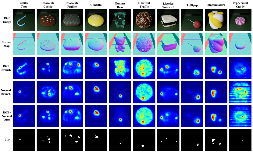
Figure 8: Qualitative results on Eyecandies. From top to bottom: the input images, the corresponding depth maps, the output anomaly maps of RGB branch, the output anomaly maps of depth branch, the output anomaly maps of CRD, and the ground truth masks.

Fig. 8 visualizes the anomaly maps generated by our proposed CRD on Eyecandies. Our method demonstrates strong sensitivity to both 2D and 3D modalities, enabling comprehensive multimodal anomaly localization.

References

- Akcay et al. [2019] Samet Akcay, Amir Atapour-Abarghouei, and Toby P Breckon. Ganomaly: Semi-supervised anomaly detection via adversarial training. In Computer Vision–ACCV 2018: 14th Asian Conference on Computer Vision, Perth, Australia, December 2–6, 2018, Revised Selected Papers, Part III 14, pages 622–637. Springer, 2019.
- Bae et al. [2023] Jaehyeok Bae, Jae-Han Lee, and Seyun Kim. Pni: industrial anomaly detection using position and neighborhood information. In Proceedings of the IEEE/CVF International Conference on Computer Vision, pages 6373–6383, 2023.
- Batzner et al. [2024] Kilian Batzner, Lars Heckler, and Rebecca König. Efficientad: Accurate visual anomaly detection at millisecond-level latencies. In Proceedings of the IEEE/CVF Winter Conference on Applications of Computer Vision, pages 128–138, 2024.
- Bergmann and Sattlegger [2023] Paul Bergmann and David Sattlegger. Anomaly detection in 3d point clouds using deep geometric descriptors. In Proceedings of the IEEE/CVF Winter Conference on Applications of Computer Vision, pages 2613–2623, 2023.
- Bergmann et al. [2018] Paul Bergmann, Sindy Löwe, Michael Fauser, David Sattlegger, and Carsten Steger. Improving unsupervised defect segmentation by applying structural similarity to autoencoders. arXiv preprint arXiv:1807.02011, 2018.
- Bergmann et al. [2019] Paul Bergmann, Michael Fauser, David Sattlegger, and Carsten Steger. Mvtec ad–a comprehensive real-world dataset for unsupervised anomaly detection. In Proceedings of the IEEE/CVF conference on computer vision and pattern recognition, pages 9592–9600, 2019.
- Bergmann et al. [2021] Paul Bergmann, Xin Jin, David Sattlegger, and Carsten Steger. The mvtec 3d-ad dataset for unsupervised 3d anomaly detection and localization. arXiv preprint arXiv:2112.09045, 2021.
- Bergmann et al. [2022] Paul Bergmann, Kilian Batzner, Michael Fauser, David Sattlegger, and Carsten Steger. Beyond dents and scratches: Logical constraints in unsupervised anomaly detection and localization. International Journal of Computer Vision, 130(4):947–969, 2022.
- Bonfiglioli et al. [2022] Luca Bonfiglioli, Marco Toschi, Davide Silvestri, Nicola Fioraio, and Daniele De Gregorio. The eyecandies dataset for unsupervised multimodal anomaly detection and localization. In Proceedings of the Asian Conference on Computer Vision, pages 3586–3602, 2022.
- Chen et al. [2023] Ruitao Chen, Guoyang Xie, Jiaqi Liu, Jinbao Wang, Ziqi Luo, Jinfan Wang, and Feng Zheng. Easynet: An easy network for 3d industrial anomaly detection. In Proceedings of the 31st ACM International Conference on Multimedia, pages 7038–7046, 2023.
- Chu et al. [2023] Yu-Min Chu, Liu Chieh, Ting-I Hsieh, Hwann-Tzong Chen, and Tyng-Luh Liu. Shape-guided dual-memory learning for 3d anomaly detection. 2023.
- Costanzino et al. [2024] Alex Costanzino, Pierluigi Zama Ramirez, Giuseppe Lisanti, and Luigi Di Stefano. Multimodal industrial anomaly detection by crossmodal feature mapping. In Proceedings of the IEEE/CVF Conference on Computer Vision and Pattern Recognition, pages 17234–17243, 2024.
- Deng and Li [2022] Hanqiu Deng and Xingyu Li. Anomaly detection via reverse distillation from one-class embedding. In Proceedings of the IEEE/CVF conference on computer vision and pattern recognition, pages 9737–9746, 2022.
- Gu et al. [2023] Zhihao Gu, Liang Liu, Xu Chen, Ran Yi, Jiangning Zhang, Yabiao Wang, Chengjie Wang, Annan Shu, Guannan Jiang, and Lizhuang Ma. Remembering normality: Memory-guided knowledge distillation for unsupervised anomaly detection. In Proceedings of the IEEE/CVF International Conference on Computer Vision, pages 16401–16409, 2023.
- Gu et al. [2024] Zhihao Gu, Jiangning Zhang, Liang Liu, Xu Chen, Jinlong Peng, Zhenye Gan, Guannan Jiang, Annan Shu, Yabiao Wang, and Lizhuang Ma. Rethinking reverse distillation for multi-modal anomaly detection. In Proceedings of the AAAI Conference on Artificial Intelligence, pages 8445–8453, 2024.
- Guo et al. [2023] Hewei Guo, Liping Ren, Jingjing Fu, Yuwang Wang, Zhizheng Zhang, Cuiling Lan, Haoqian Wang, and Xinwen Hou. Template-guided hierarchical feature restoration for anomaly detection. In Proceedings of the IEEE/CVF International Conference on Computer Vision, pages 6447–6458, 2023.
- Guo et al. [2024] Jia Guo, Lize Jia, Weihang Zhang, Huiqi Li, et al. Recontrast: Domain-specific anomaly detection via contrastive reconstruction. Advances in Neural Information Processing Systems, 36, 2024.
- Horwitz and Hoshen [2023] Eliahu Horwitz and Yedid Hoshen. Back to the feature: classical 3d features are (almost) all you need for 3d anomaly detection. In Proceedings of the IEEE/CVF Conference on Computer Vision and Pattern Recognition, pages 2968–2977, 2023.
- Li et al. [2021] Chun-Liang Li, Kihyuk Sohn, Jinsung Yoon, and Tomas Pfister. Cutpaste: Self-supervised learning for anomaly detection and localization. In Proceedings of the IEEE/CVF conference on computer vision and pattern recognition, pages 9664–9674, 2021.
- Li et al. [2024] Hanxi Li, Jianfei Hu, Bo Li, Hao Chen, Yongbin Zheng, and Chunhua Shen. Target before shooting: Accurate anomaly detection and localization under one millisecond via cascade patch retrieval. IEEE Transactions on Image Processing, 2024.
- Lin and Yan [2024] Jiang Lin and Yaping Yan. A comprehensive augmentation framework for anomaly detection. In Proceedings of the AAAI Conference on Artificial Intelligence, pages 8742–8749, 2024.
- Liu et al. [2024] Jiaqi Liu, Guoyang Xie, Ruitao Chen, Xinpeng Li, Jinbao Wang, Yong Liu, Chengjie Wang, and Feng Zheng. Real3d-ad: A dataset of point cloud anomaly detection. Advances in Neural Information Processing Systems, 36, 2024.
- Roth et al. [2022] Karsten Roth, Latha Pemula, Joaquin Zepeda, Bernhard Schölkopf, Thomas Brox, and Peter Gehler. Towards total recall in industrial anomaly detection. In Proceedings of the IEEE/CVF Conference on Computer Vision and Pattern Recognition, pages 14318–14328, 2022.
- Rudolph et al. [2023] Marco Rudolph, Tom Wehrbein, Bodo Rosenhahn, and Bastian Wandt. Asymmetric student-teacher networks for industrial anomaly detection. In Proceedings of the IEEE/CVF winter conference on applications of computer vision, pages 2592–2602, 2023.
- Salehi et al. [2021] Mohammadreza Salehi, Niousha Sadjadi, Soroosh Baselizadeh, Mohammad H Rohban, and Hamid R Rabiee. Multiresolution knowledge distillation for anomaly detection. In Proceedings of the IEEE/CVF conference on computer vision and pattern recognition, pages 14902–14912, 2021.
- Tien et al. [2023] Tran Dinh Tien, Anh Tuan Nguyen, Nguyen Hoang Tran, Ta Duc Huy, Soan Duong, Chanh D Tr Nguyen, and Steven QH Truong. Revisiting reverse distillation for anomaly detection. In Proceedings of the IEEE/CVF conference on computer vision and pattern recognition, pages 24511–24520, 2023.
- Wang et al. [2021] Guodong Wang, Shumin Han, Errui Ding, and Di Huang. Student-teacher feature pyramid matching for anomaly detection. In 32nd British Machine Vision Conference 2021, BMVC 2021, Online, November 22-25, 2021, page 306. BMVA Press, 2021.
- Wang et al. [2023] Yue Wang, Jinlong Peng, Jiangning Zhang, Ran Yi, Yabiao Wang, and Chengjie Wang. Multimodal industrial anomaly detection via hybrid fusion. In Proceedings of the IEEE/CVF Conference on Computer Vision and Pattern Recognition, pages 8032–8041, 2023.
- Zagoruyko and Komodakis [2016] Sergey Zagoruyko and Nikos Komodakis. Wide residual networks. arXiv preprint arXiv:1605.07146, 2016.
- Zavrtanik et al. [2021] Vitjan Zavrtanik, Matej Kristan, and Danijel Skočaj. Draem-a discriminatively trained reconstruction embedding for surface anomaly detection. In Proceedings of the IEEE/CVF International Conference on Computer Vision, pages 8330–8339, 2021.
- Zavrtanik et al. [2024a] Vitjan Zavrtanik, Matej Kristan, and Danijel Skočaj. Cheating depth: Enhancing 3d surface anomaly detection via depth simulation. In Proceedings of the IEEE/CVF Winter Conference on Applications of Computer Vision, pages 2164–2172, 2024a.
- Zavrtanik et al. [2024b] Vitjan Zavrtanik, Matej Kristan, and Danijel Skočaj. Keep dræming: Discriminative 3d anomaly detection through anomaly simulation. Pattern Recognition Letters, 181:113–119, 2024b.
- Zhang et al. [2024] Jie Zhang, Masanori Suganuma, and Takayuki Okatani. Contextual affinity distillation for image anomaly detection. In Proceedings of the IEEE/CVF Winter Conference on Applications of Computer Vision, pages 149–158, 2024.
- Zhang et al. [2023] Xinyi Zhang, Naiqi Li, Jiawei Li, Tao Dai, Yong Jiang, and Shu-Tao Xia. Unsupervised surface anomaly detection with diffusion probabilistic model. In Proceedings of the IEEE/CVF International Conference on Computer Vision, pages 6782–6791, 2023.
- Zou et al. [2022] Yang Zou, Jongheon Jeong, Latha Pemula, Dongqing Zhang, and Onkar Dabeer. Spot-the-difference self-supervised pre-training for anomaly detection and segmentation. In European Conference on Computer Vision, pages 392–408. Springer, 2022.