Deep Clustering using Dirichlet Process Gaussian Mixture and Alpha Jensen-Shannon Divergence Clustering Loss

Abstract

Deep clustering is an emerging topic in deep learning where traditional clustering is performed in deep learning feature space. However, clustering and deep learning are often mutually exclusive. In the autoencoder based deep clustering, the challenge is how to jointly optimize both clustering and dimension reduction together, so that the weights in the hidden layers are not only guided by reconstruction loss, but also by a loss function associated with clustering. The current state-of-the-art has two fundamental flaws. First, they rely on the mathematical convenience of Kullback-Leibler divergence for the clustering loss function but the former is asymmetric. Secondly, they assume the prior knowledge on the number of clusters is always available for their dataset of interest. This paper tries to improve on these problems. In the first problem, we use a Jensen-Shannon divergence to overcome the asymmetric issue, specifically using a closed form variant. Next, we introduce an infinite cluster representation using Dirichlet process Gaussian mixture model for joint clustering and model selection in the latent space which we called deep model selection. The number of clusters in the latent space are not fixed but instead vary accordingly as they gradually approach the optimal number during training. Thus, prior knowledge is not required. We evaluate our proposed deep model selection method with traditional model selection on large class number datasets such as MIT67 and CIFAR100 and also compare with both traditional variational Bayes model and deep clustering method with convincing results.

I Introduction

One of the key success of deep learning is attributed to the feature extraction capability that is found in the first several hidden layers of the network. Deep clustering is an emerging topic in deep learning where traditional clustering is performed in deep learning feature space. However, clustering and deep learning are often mutually exclusive. Deep learning is seen as a black box and the non-linearity of the network remains mathematically unclear to the researcher. Traditional clustering method such as Kmeans or GMM while mathematically sound is very hard to extend to deep layer representation. A recent technique known as deep clustering tries to bridge both sides by the simple use of a minimization between the network weights and clustering parameters. According to literature [1], we can categorize deep clustering by their network architecture: autoencoder [2, 3, 4, 5, 6], generative adversarial network [7, 8] and convolutional neural network [9, 10].

In particular, we only focus on the autoencoder category which is the simplest but performance wise is not necessarily inferior to the other two categories [1]. Within this category, the Type II regularizer in Table I (also referred to as the clustering loss in [1]) is the basis for deep clustering. An autoencoder (AE) maps an input to a point in a reduced dimension latent space using reconstruction loss. Dimension reduction is important for image clustering since a more compact representation can usually improve the accuracy. Specifically, Autoencoder Based Clustering (ABC) [2, 11] proposed a Type II regularizer to minimize the difference between an image encoded as a point in the latent space and its nearest cluster mean. The latter is computed using Kmeans in the entire latent space. When backpropagating from this regularizer, the encoder weights will restructure itself to output a latent space that mimics a partition performed by Kmeans. We can achieve better clustering this way than either Kmeans or autoencoder alone. In such approach, there are two objectives to be solved, i.e. the network weights and the cluster parameters. Thus in practice, we alternate between each optimization while fixing the other.

Along the way, self-expressiveness and sparse coding were proposed on top of ABC’s loss [12, 13]. Later on, Gaussian mixture model (GMM) and Variational Autoencoder (VAE) quickly became very popular for deep clustering [14] but remains unclear. The latest installment in this direction [5, 4, 15, 16] uses the Kullback-Leibler divergence (KLD) between VAE and GMM to define the Type II regularizer. Unlike the ABC’s Type II regularizer which is a point estimate version, the KLD approach is a powerful representation since the performance can vary depending on the probabilistic model used. Yet there are two main issues that are left out with the latest installment of KLD based methods.

 

Problem statement:

1) KLD is asymmetrical and undefined when one of the probability distribution is zero.

2) The number of cluster is a prior knowledge that is required beforehand in deep clustering.

 

The first issue will be problematic when there are regions in the latent space that are left out by the network when they actually fall under GMM coverage. This will lead to no gradient learnt for these specific region. The second issue is that deep clustering are mostly reported on trival cases such as 4 or 10 classes. When presented with an unknown dataset, there is no easy way to know what is the optimal number of clusters to set for deep clustering. Even if we resort to well known technique like cross validation or Bayesian information criteria, these methods are standalone techniques and do not jointly optimize deep clustering. Also, the application of deep clustering will be severely limited as a wrong decision on the number of clusters will lead to much worse result than traditional clustering alone.

 

Contributions:

1) We use Jensen-Shannon divergence for the loss function since it is symmetrical and always defined.

2) Dirichlet process Guassian mixture is used to jointly perform both deep clustering and model selection.

 

There is no closed form solution for the Jensen-Shannon divergence (JSD) of two Gaussians. As a workaround, we use a recent work known as the $\alpha$JSD in [17] which rely on an input skew parameter $\alpha$ to allow JSD to derive a closed form solution. We also discuss a simpler form of $\alpha$JSD which is essentially a first order solution i.e. cluster mean only. We propose using Dirichlet process mixture (DPM) [18] which is a type of Bayesian nonparametic model for clustering. The main difference between DPM and GMM lies in the infinite number of cluster representation. This means that we do not need to specify exactly the number of clusters to be used. Instead, we fix a sufficiently large truncated value for the infinite number of clusters. Also, the Bayesian approach to DPM allows prior assumption over the latent space. Thus, data overfitting and cluster singularities are simultaneously addressed [19]. This is not possible with the standard GMM in [5, 4].

I-A Related work

TABLE I: Types of loss functions used in autoencoder

Objective	Methods	Reconst. Loss	Type I Regularizer Loss	Type II Regularizer Loss
RC
	AE [20]	$p(x|z)$	-	-
RC+PR	VAE [21]	$p(x|z)$	$KLD\left[q(z\mid x)\parallel p(z)\right]$	-
RC+PR+CL
	VAED [16]	$p(x|z)$	$KLD\left[q(z\mid x)\parallel p(z)\right]$	$KLD\left[q(z\mid x)\parallel p(z\mid\theta^{*})\right]$
RC+CL+MS	This work	$p(x|z)$	-	$JSD\left[q(z\mid x)\parallel p(z\mid\phi^{*})\right]$

(RC, PR, CL, MS refers to reconstruction, prior representation, clustering and model selection respectively)

Table I summarizes some recent works related to this paper, notably AE, VAE and VAED. Type I regularizer enforces the latent space of the autoencoder to follow a prior distribution. Thus, we can generate a sample in the latent space using a random number generator (associated with the prior). The Type II regularizer minimizes the within class distance in the latent space based on a classical clustering algorithm such as Kmeans. Thus, samples coming from the same cluster will be densely distributed in the latent space, allowing more discriminative class pattern to be picked up later. Both Type I and II regularizers are mutually exclusive and can be trained separately. In this work, we mainly focus on the Type II regularizer. The works of VaDE and VAED [4, 16] are based on the KLD representation of ABC [2] while DGG [5] based on the JSD representation of ABC. However, since there is no closed form approach to JSD, the authors of DGG proposed a heuristic approach to JSD. DPM has also been proposed by Ye et al [22] for VAE. However, the problem Ye et al is solving is subspace clustering which is different from deep model selection. Their goal is to automatically find the number of subspaces using DPM. Whereas, we are finding the number of clusters to represent the entire latent space. In VaDE, the underlying prior distribution is based on the original VAE i.e. Gaussian distributed. In SB-VAE [23], the authors model VAE’s Type I regularizer with a Dirichlet process prior. In VSC-DVM [15], the authors proposed using SB-VAE’s Type I regularizer and VaDE’s Type II regularizer. Objectively, the authors of VSC-DVM were solving finite cluster representation in the latent space. To the best of our knowledge, it is uncommon to find model selection in Type II regularizer.

II Methodology

II-A Infinite number of clusters for representing latent space

We begin with the simplest Type II regularizer known as the ABC loss in [2]. An autoencoder (AE) learns to represent an image in the reduced dimension latent space by minimizing the reconstruction loss (using the mean square error, MSE) between a input $x$ and network output $y$ as seen in the first term of eqn (1).

$$\begin{array}[]{c}\mathcal{L_{MSE}}+\mathcal{L_{ABC}}\\ \\ =\ln p(x|z)-\lambda_{3}\left\|\eta^{*}-z\right\|^{2}\\ \\ =-\frac{1}{2}\left(x-y\right)^{2}-\frac{\lambda_{3}}{2}\left(\eta^{*}-z\right)^{2}\end{array}$$ (1)

A simple yet effective way to optimize both dimensionality reduction and clustering is to introduce a second term in eqn (1) as proposed recently by [2]. The second term or the Type II regularizer tries to enforce the latent space to exhibit a Kmeans like partitioning. More specifically in eqn (1): Given an input image $x_{n}$, we use the encoder to obtain a point, $z_{n}$ in the latent space. We first use Kmeans to partition the latent space into $K$ clusters. Then, we use the cluster assignment of Kmeans to find the nearest cluster mean $\eta^{*}$ to the point $z_{n}$ in the latent space. Backpropagating on this regularizer will affect the encoder weights $w$ to output a re-structured latent space that mimic a partitioning performed by Kmeans. The parameter $\lambda_{3}$ reduces the effect of the regularizer on the encoder weights updates. The parameter $\lambda_{3}$ is set to $[0,1]$.

In the above ABC approach, we are required to predefine the number of clusters or $K$ to represent the latent space of the autoencoder, whose mean are defined as $\eta=\left\{\eta{}_{k}\right\}_{k=1}^{K}\in\mathbb{R}{}^{D}$ (The total dimension of each observed instance is denoted $D$). Instead of predefining $K$, we would like to automatically find $K$. This is especially helpful when we do not have label information for a given dataset we wish to perform ABC. First, we represent the same latent space using an infinite number of clusters $\eta=\left\{\eta{}_{k}\right\}_{k=1}^{\infty}\in\mathbb{R}{}^{D}$. Ideally, we would like to have a handful of dominating clusters that carry larger weightage of information, $v=\left\{v_{k}\right\}_{k=1}^{\infty}\in\mathbb{R}$ to represent the entire latent space. As we gradually approach the other end of the spectrum, we would like to see a lot of redundant clusters with lower weightage of information. These redundant clusters will be slowly pruned away by optimization. When we plot the frequency of this spectrum, we should observe a decaying distribution best modeled by a Dirichlet distribution or $v\sim Beta(1,a_{0})$. We can normalize the weightage using $\pi_{k}=v_{k}\prod_{l=1}^{k-1}\left(1-v_{k}\right)$ such that the sum of these normalized weightage across the spectrum gives a unit measure i.e. $\sum_{k=1}^{\infty}\pi_{k}=1$ as given by [24]. This autoencoder latent space representation of using an infinite number of clusters is one of the key concept in this paper.

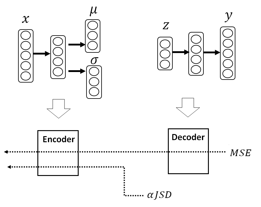
Figure 1: Deep model selection using proposed loss function $\alpha JSD$.

II-B Regularizing autoencoder with infinite number of clusters

We refer to the Type II regularizer used by deep clustering methods e.g. [4, 15, 16] in eqn (2). $q(z\mid x)$ is a single point in the VAE latent space which follows a Gaussian distribution and $p(z\mid\theta^{*})$ is the GMM estimated on the entire VAE latent space. A random sample in the VAE latent space is defined by Kingma et al [21] as $z=\mu+\sigma\cdot\mathcal{N}(0,1).$ Both $\mu$ and $\sigma$ are the hidden layers of an autoencoder. To recover an autoencoder from VAE, we simply discard $\sigma$. On the other hand, we define $\theta=\left\{\eta,\tau,\psi\right\}$ as the GMM mean, precision and soft assignment. The cluster assignment is denoted $\varsigma=\left\{\varsigma_{n}\right\}_{n=1}^{N}$ where $\varsigma_{n}$ is a $1-of-K$ binary vector, subjected to $\sum_{k=1}^{K}\varsigma_{nk}=1$ and $\varsigma_{nk}\in\left\{0,1\right\}$. $\theta^{*}$ refers to the parameters of the optimal GMM cluster, given a particular sample in the latent space, $z_{n}$. It is found by the cluster assignment $\varsigma_{n}$, using eqn (2).

$$\begin{array}[]{c}{KLD}\left[q(z\mid x)\parallel p(z\mid\theta^{*})\right]\\ \\ \theta^{*}=\underset{k}{\arg\max}\;\left\{\ln\mathcal{N}\left(z_{n}\mid\eta_{k},\tau_{k}\right)^{\varsigma_{nk}}+\left(\ln\psi_{k}\right)^{\varsigma_{nk}}\right\}\end{array}$$ (2)

In most VAE based deep clustering e.g. [15], the authors assume $\psi_{k}=\frac{1}{K}$ i.e. each cluster has equal sample count. Thus, the second term in $\theta^{*}$ can be discarded when computing the regularizer in eqn (2).

Next, we extend the Type II regularizer to DPM as denoted by $p(z\mid\phi^{*})$ in eqn (3) and also illustrated in Figure 1. We further define $\phi=\left\{\eta,\tau,v\right\}$ as the DPM mean, precision, and cluster weightage. The cluster assignment is also denoted $\varsigma$. The meaning of $\phi^{*}$ is similar to $\theta^{*}$ where the optimal DPM parameters is found by solving the DPM cluster assignment in eqn (3).

$$\begin{array}[]{c}{KLD}\left[q(z\mid x)\parallel p(z\mid\phi^{*})\right]\\ \\ \phi^{*}=\underset{k}{\arg\max}\left\{\underset{\eta_{k},\tau_{k},v_{k}}{E}\left[\ln\mathcal{N}(z_{n}\mid\eta_{k},\tau_{k})^{\varsigma_{nk}}\right.\right.\\ \\ \left.\left.+\left(\ln v_{k}\right)^{\varsigma_{nk}}+\sum_{l=1}^{k-1}\left(\;\ln(1-v_{l})\;\right)^{\varsigma_{nk}}\right]\right\}\end{array}$$ (3)

One of the main difference between deep clustering in (2) and deep model selection in (3) can be attributed to the difference between $\psi_{k}=\frac{1}{K}$ in eqn (2) and $\pi_{k}=v_{k}\prod_{l=1}^{k-1}(1-v_{l})$ in eqn (3). The cluster size of the former is $1\ldots k\ldots K$ and the latter is $1\ldots k\ldots\infty$. Moreover, in the graphical representation between GMM and DPM in Figure 3, we can see that the DPM parameters in deep model selection rely on prior assumptions and are in turn governed by several hyperparameters. In Fig 3, $\omega_{0}$ is the hyperparameter of the Beta distributed prior for cluster weightage. Likewise, $\lambda_{0}$ and $m_{0}$ correspond to the Gaussian distributed prior for cluster mean and $a_{0},b_{0}$ are for the Gamma distributed prior for precision.

II-C Type II Regularizer using $\alpha$JS divergence

It is recently shown in [16] that when we re-express the ABC objective as a KLD between GMM and VAE encoder output i.e. between two Gaussians, a generic closed form solution is available

$$\begin{array}[]{c}{KLD}\left[q(z\mid x)\parallel p(z\mid\theta^{*})\right]\\ \\ ={KLD}\left[\mathcal{N}(\mu,\sigma)\parallel\mathcal{N}(\eta^{*},\tau^{*})\right]\\ \\ =\ln\tau^{*}+\ln\sigma+\frac{\left(\tau^{*}\right)^{-1}+\left(\eta^{*}-\mu\right)^{2}}{2\sigma_{2}}-\frac{1}{2}\end{array}$$ (4)

Unlike the KLD of two Gaussians, there is no closed-form solution for JSD. The authors in [5] propose a JSD for the ABC objective based on an upper bound constraint. The former is essentially an average sum between two standard KLD of eqn (2). Instead, we consider another form of JSD which we called the $\alpha$JSD: In Nielsen [17], the use of a skew parameter $\alpha$ allows the JSD to possess a closed form solution between two Gaussians as quoted in eqn (5)

$$\begin{array}[]{c}{\alpha JSD}\left[\mathcal{N}(\mu_{1},\sigma_{1})\parallel\mathcal{N}(\mu_{2},\sigma_{2})\right]\\ \\ =\left(1-\alpha\right)\left(\mu_{\alpha}-\mu_{1}\right)^{2}\sigma_{\alpha}^{-1}+\alpha\left(\mu_{\alpha}-\mu_{2}\right)^{2}\sigma_{\alpha}^{-1}\\ \\ -d+\frac{1}{2}\sum\left(\sigma_{\alpha}^{-1}\left(1-\alpha\right)\sigma_{1}+\alpha\sigma_{2}\right)+\log\frac{\sigma_{\alpha}}{\sigma_{1}^{1-\alpha}\sigma_{2}^{\alpha}}\\ \\ \end{array}$$ (5)

Unlike KLD in eqn (4), $\alpha$JSD further rely on skew variables for the first and second order variables as follows [17]

$$\begin{array}[]{c}\sigma_{\alpha}=\left(\sigma_{1}^{-1}\left(1-\alpha\right)+\sigma_{2}^{-1}\alpha\right)^{-1}\\ \\ \mu_{\alpha}=\sigma_{\alpha}\left(\sigma_{1}^{-1}\mu_{1}\left(1-\alpha\right)+\sigma_{2}^{-1}\mu_{2}\alpha\right)\\ \\ \end{array}$$ (6)

For eqn (5) and (6), we refer to $\left(\mu_{1},\sigma_{1}\right)$ and $\left(\mu_{2},\sigma_{2}\right)$ as network variable $\left(\mu,\sigma\right)$ and DPM variable $\left(\eta^{*},\tau^{*}\right)$ respectively.

The symmetrical property of JSD can be explained using eqn (6). For explanation purpose, we can assume the simple case of first order variable only i.e. ignore $\left(\sigma_{1},\sigma_{2}\right)$. When we consider the case of KLD in eqn (4), we arrive at the following form $KLD=\frac{1}{2}\left(\mu_{1}-\mu_{2}\right)^{2}$. When we have the network variable $\mu_{2}$ outputting a near zero, we end up with a large value for KLD e.g. $KLD=0.5\left(\mu_{1}\right)^{2}$. This is the main cause of asymmetry in KLD. On the other hand, we compare the case where $\alpha JSD=\left(1-\alpha\right)\left(\mu_{\alpha}-\mu_{1}\right)^{2}+\alpha\left(\mu_{\alpha}-\mu_{2}\right)^{2}$ and $\mu_{\alpha}=\left(\mu_{1}\left(1-\alpha\right)+\mu_{2}\alpha\right)$. Again when we assume $\mu_{2}\rightarrow 0$ and $0\leq\alpha\leq 1$, we observe that $\alpha JSD\ll KLD$ as seen in Fig 2. Thus, the choice of $\alpha$ can alleviate $\alpha JSD$ from the asymmetry problem that plagues KLD. For a working case, when both $\mu_{1},\mu_{2}$ have similar values, both KLD and $\alpha$JSD should correctly be computing a value close to zero as seen in Fig 2.

 

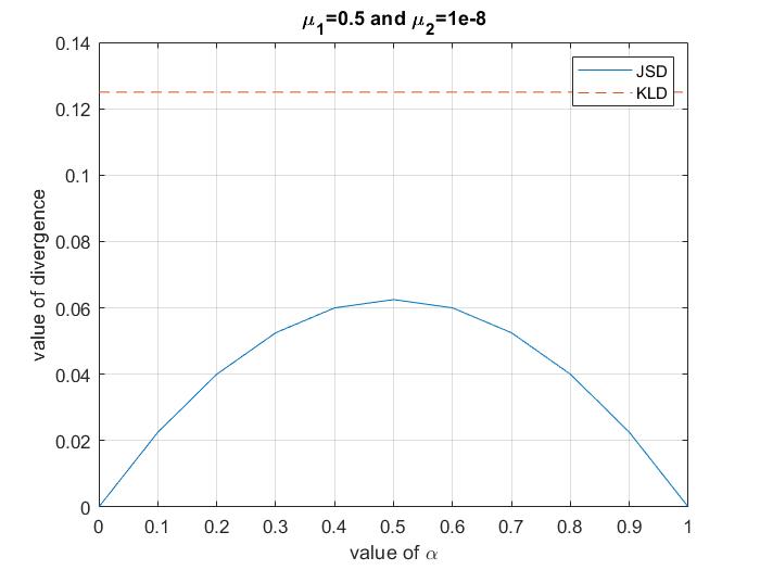
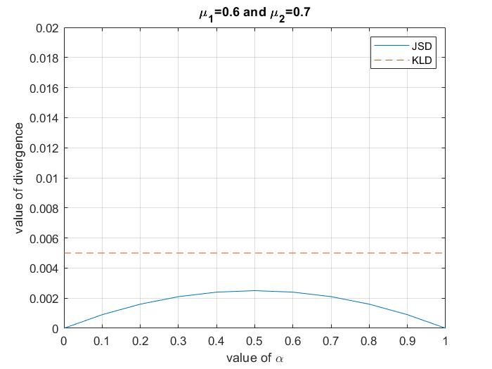
Figure 2: The asymmetry problem in KLD vs $\alpha$JSD

II-D Variational inference of Dirichlet process Gaussian mixture

In the standard GMM as shown in Fig 3, the hidden variables are updated by the point estimates, $\hat{\tau_{k}},\hat{\eta_{k}},\hat{\varsigma_{nk}},\hat{\psi_{k}}$. The expectation-maximization algorithm allows us to obtain point estimates using the closed form equations [19, 25] below

$$\begin{array}[]{c}\hat{\tau_{k}}=\left\{\frac{1}{2}\sum_{n=1}^{N}\varsigma_{nk}\right\}/\\ \left\{\frac{1}{2}\left(\sum_{n=1}^{N}(z_{n}-\eta_{k})^{2}\varsigma_{nk}\right)\right\}\\ \\ \end{array}$$ (7)

$$\begin{array}[]{c}\hat{\eta_{k}}=\left\{\sum_{n=1}^{N}\varsigma_{nk}z_{n}\right\}/\left\{\sum_{n=1}^{N}\varsigma_{nk}\right\}\\ \\ \end{array}$$ (8)

$$\begin{array}[]{c}\hat{\varsigma_{nk}}=\underset{k}{\arg\max}\;\left\{\ln\psi_{k}-\frac{1}{2}\left(z_{n}-\eta_{k}\right){}^{2}\right\}\varsigma_{nk}\\ \\ \end{array}$$ (9)

$$\begin{array}[]{c}\hat{\psi_{k}}=\left\{\sum_{n=1}^{N}\varsigma_{nk}\right\}/\left\{\sum_{k=1}^{K}\sum_{n=1}^{N}\varsigma_{nk}\right\}\\ \\ \end{array}$$ (10)

In the variational Bayesian approach, each hidden variable is modeled as a posterior distribution. According to variational inference [19], each posterior is updated by computing its posterior expectation. The optimal posteriors of Bayesian DPM can be defined through their expectations below in [26] as follows

$$\begin{array}[]{c}E\left[\tau_{k}\right]^{\prime}=\left\{\frac{1}{2}\sum_{n=1}^{N}E\left[\varsigma_{nk}\right]+\left(a_{0}-1\right)\right\}/\\ \left\{b_{0}+\frac{1}{2}\left(\sum_{n=1}^{N}(z_{n}-E\left[\eta_{k}\right])^{2}E\left[\varsigma_{nk}\right]+\lambda_{0}(E\left[\eta_{k}\right]-m{}_{0})^{2}\right)\right\}\\ \\ \end{array}$$ (11)

$$\begin{array}[]{c}E\left[\eta_{k}\right]^{\prime}=\left\{\sum_{n=1}^{N}E\left[\varsigma_{nk}\right]z_{n}+\lambda_{0}m_{0}\right\}/\\ \left\{\sum_{n=1}^{N}E\left[\varsigma_{nk}\right]+\lambda_{0}\right\}\\ \\ \end{array}$$ (12)

$$\begin{array}[]{c}E\left[\varsigma_{nk}\right]^{\prime}=\underset{\varsigma_{nk}}{\arg\max}\;\left\{-\frac{1}{2}\left(z_{n}-E\left[\eta_{k}\right]\right){}^{2}+\ln E\left[v_{k}\right]\right.\\ \left.+\sum_{l=1}^{k-1}\ln(1-E\left[v_{l}\right])\right\}\varsigma_{nk}\\ \\ \end{array}$$ (13)

$$\begin{array}[]{c}E\left[v_{k}\right]^{\prime}=\left\{\sum_{n=1}^{N}E\left[\varsigma_{nk}\right]\right\}/\\ \left\{\sum_{n=1}^{N}\sum_{j=k+1}^{K}E\left[\varsigma_{nj}\right]+\omega_{0}-1\right\}\\ \\ \end{array}$$ (14)

The above hyperparameters $\lambda_{0},m_{0},\omega_{0},a_{0},b_{0}$ can either be found empirically or treated as noninformative priors for convenience. Earlier we have discussed on the cluster weightage, $v=\left\{v_{k}\right\}_{k=1}^{T}\in\mathbb{R}{}^{Z}$ in DPM, which is responsible for model selection, as seen in Fig 3. The truncation level $T$ refers to the initial value on the largest cluster size we set (e.g. $T<100$ for MIT67). In [19], the $k$ clusters which are significant will show large values in $v_{k}$ and vice versa. By observing $v_{k}$, we can discard the redundant clusters with insignificant values. When $v$ has reach optimal training, $T$ approaches the ground truth value of $K$. This will also affect cluster mean $\eta_{k}$, cluster precision $\tau_{k}$ and cluster assignment $\varsigma_{nk}$. This is known as cluster prunning. Similarly, we can use $\psi=\left\{\psi_{k}\right\}_{k=1}^{T}\in\mathbb{R}{}^{Z}$ for GMM and apply the cluster prunning approach.

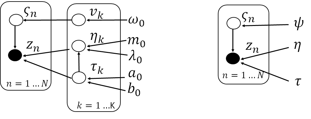
Figure 3: Graphical representation of DPM used in proposed deep model selection (left) vs GMM used in deep clustering by other works (right).

III Experiments

III-A Unsupervised methods for comparison

We compare our proposed method on image classification datasets with the following methods. DPM: Our baseline by learning DPM directly on raw feature space, using eqn (11)-(14). KLD: The method described using eqn (4) and eqn (7)-(10), which is KLD loss [16] using GMM. $\alpha$JSD: Our proposed method based on JSD loss using Bayesian DPM in eqn (5), (6) and eqn (11)-(14).

III-B Setup

Network: We train MSE loss and $\alpha JSD$ loss separately for the network. Starting with random weights for the encoder and decoder, we use MSE loss to train the encoder. Then, we use $\alpha JSD$ loss to further train the encoder. We use a learning rate of 0.01 for the encoder with two hidden layers, i.e. $512-384-256-128$. Most deep clustering methods perform all three tasks i.e. feature extraction, dimension reduction and Type II regularizer on the same encoder’s two or three hidden layers. It is actually harder to perform deep clustering this way as the encoder weights used for different dataset have to be pretrained or tuned differently. Some of the best results of these deep clustering methods require dedicated tuning. We compensate for our lack of depth in the network using pretrained ResNet as the feature extractor. In some datasets where the image is real, some authors also use this strategy e.g. VaDE [12] use ResNet50 for STL-10. We only demonstrated end-to-end on MNIST, i.e. using raw pixel. For the other datasets, we solely use ResNet18 pretrained on ImageNet. Each image after ResNet18 feature extraction has a dimension 1x512. The $\alpha JSD$ parameter $\lambda_{3}=1$. We typically fix $\alpha=0.65$ in eqn (6) to enable more biasing towards DPM for the learning of the network weights. DPM: The hyperparameters we use are $\omega_{0}=2000$, $a_{0}=1.25$ $b_{0}=0.25$, $m_{0}=1$ and $\lambda_{0}=0.5$. The DPM truncation levels are set at $T=200$ (CIFAR100), $T=100$ (MIT67) and at $T=50$ (CIFAR10). We also use Kmeans for initialization.

III-C Experimental Results

We refer the reader to [16, 27] for more details on the datasets used in this work i.e. CIFAR10, MIT67, and CIFAR100. We use Accuracy (ACC) for clustering as defined in [28] to evaluate the performance of our method. We rerun our experiments at least 10 rounds and take the average result in Table II.

CIFAR10: Most clustering papers do not directly use the raw pixels in CIFAR10 for clustering. Thus, we use ImageNet pretrained ResNet18 (on CIFAR10) as the image feature for DPM and $\alpha JSD$. As a direct comparison, our baseline using DPM is able to obtain ACC at 0.7941 while, $\alpha JSD$ is able to outperform DPM while having more closely estimated cluster size, $\hat{K}$. For ACC, $\alpha JSD$ is slightly better than $KLD$ for CIFAR10.

MIT67: MIT67 has 67 classes and lesser number of samples than CIFAR10. It is quite useful as an intermediate dataset for deep clustering and model selection task. However as the real images are very complex, most deep clustering which use encoder for feature extraction are unable to cope with this dataset. Instead, we use ImageNet pretrained ResNet18 as the image feature. The estimated cluster size, $\hat{K}$ of $\alpha JSD$ is slightly poorer than DPM as there are much fewer samples per class for this dataset than CIFAR10. But $\alpha JSD$ outperforms KLD in terms of ACC in this dataset. Overall $\alpha JSD$ is able to obtain the best performance.

CIFAR100: This is a challenging dataset as it has a fairly large number of classes. It is difficult to find papers that target beyond 10 or 20 classes. Furthermore, the raw pixels in CIFAR100 are unsuitable for direct use as the object classification dataset contains real images distorted by many image variance. Similarly, we also use a ImageNet pretrained ResNet18 (on CIFAR100) as the image feature so as to boost up the feature discrimination. $\alpha JSD$ is able to consistently outperform all baselines in terms of ACC and the estimated cluster size. Lastly, $\alpha JSD$ demonstrates that $\alpha$JSD performs better than KLD in this dataset for ACC.

TABLE II: Experimental results

	CIFAR10			MIT67			CIFAR100
	ACC	$\hat{K}$		ACC	$\hat{K}$		ACC	$\hat{K}$
DPM	0.7941	17		0.6121	81		0.5753	150
$KLD$	0.8834	12		0.70426	85		0.6145	118
$\alpha JSD$	0.8845	12		0.71906	83		0.6221	119

IV Conclusion

In this paper we discussed about deep clustering, a type of deep learning which performs traditional clustering in deep learning feature space using VAE. The state-of-the-art in this category is a method known as VaDE. The problem VaDE tries to solve is how to use a KLD representation for VAE and GMM. The problem we try to solve is how to use a JSD representation for VAE and DPM. The novelty of using JSD is that the regularizer is symmetric and always defined unlike KLD. The problem underlying JSD is that no closed form solution is available. Thus, we introduced a new variant of JSD known as the $\alpha$JSD to overcome this problem. When using GMM for clustering, the number of clusters is required to be defined. Instead of GMM, we proposed using DPM for $\alpha$JSD which allows joint model selection and deep clustering. We call this approach as deep model selection. Lastly, we compare our proposed approach with both KLD using GMM and variational Bayes DPM on several large class number datasets with convincing results. A possible future work could be to exploit the neighborhood information of images for training the latent space of VAE. This would require using different types of regularization for VAE as discussed in Table I.

References

- [1] E. Min, X. Guo, Q. Liu, G. Zhang, J. Cui, and J. Long, “A survey of clustering with deep learning: From the perspective of network architecture,” IEEE Access, vol. 6, pp. 39 501–39 514, 2018.
- [2] C. Song, F. Liu, Y. Huang, L. Wang, and T. Tan, “Auto-encoder based data clustering,” in Iberoamerican Congress on Pattern Recognition. Springer, 2013, pp. 117–124.
- [3] J. Xie, R. Girshick, and A. Farhadi, “Unsupervised deep embedding for clustering analysis,” in International conference on machine learning, 2016, pp. 478–487.
- [4] Z. Jiang, Y. Zheng, H. Tan, B. Tang, and H. Zhou, “Variational deep embedding: an unsupervised and generative approach to clustering,” in Proceedings of the 26th International Joint Conference on Artificial Intelligence. AAAI Press, 2017, pp. 1965–1972.
- [5] L. Yang, N.-M. Cheung, J. Li, and J. Fang, “Deep clustering by gaussian mixture variational autoencoders with graph embedding,” in Proceedings of the IEEE International Conference on Computer Vision, 2019, pp. 6440–6449.
- [6] X. Yang, C. Deng, F. Zheng, J. Yan, and W. Liu, “Deep spectral clustering using dual autoencoder network,” in Proceedings of the IEEE Conference on Computer Vision and Pattern Recognition, 2019, pp. 4066–4075.
- [7] P. Zhou, Y. Hou, and J. Feng, “Deep adversarial subspace clustering,” in Proceedings of the IEEE Conference on Computer Vision and Pattern Recognition, 2018, pp. 1596–1604.
- [8] K. Ghasedi, X. Wang, C. Deng, and H. Huang, “Balanced self-paced learning for generative adversarial clustering network,” in Proceedings of the IEEE Conference on Computer Vision and Pattern Recognition, 2019, pp. 4391–4400.
- [9] C.-C. Hsu and C.-W. Lin, “Cnn-based joint clustering and representation learning with feature drift compensation for large-scale image data,” IEEE Transactions on Multimedia, vol. 20, no. 2, pp. 421–429, 2017.
- [10] M. Caron, P. Bojanowski, A. Joulin, and M. Douze, “Deep clustering for unsupervised learning of visual features,” in Proceedings of the European Conference on Computer Vision (ECCV), 2018, pp. 132–149.
- [11] B. Yang, X. Fu, N. D. Sidiropoulos, and M. Hong, “Towards k-means-friendly spaces: Simultaneous deep learning and clustering,” in Proceedings of the 34th International Conference on Machine Learning-Volume 70. JMLR. org, 2017, pp. 3861–3870.
- [12] P. Ji, T. Zhang, H. Li, M. Salzmann, and I. Reid, “Deep subspace clustering networks,” in Advances in Neural Information Processing Systems, 2017, pp. 24–33.
- [13] J. Sun, X. Wang, N. Xiong, and J. Shao, “Learning sparse representation with variational auto-encoder for anomaly detection,” IEEE Access, vol. 6, pp. 33 353–33 361, 2018.
- [14] N. Dilokthanakul, P. A. Mediano, M. Garnelo, M. C. Lee, H. Salimbeni, K. Arulkumaran, and M. Shanahan, “Deep unsupervised clustering with gaussian mixture variational autoencoders,” arXiv preprint arXiv:1611.02648, 2016.
- [15] X. Yang, Y. Yan, K. Huang, and R. Zhang, “Vsb-dvm: An end-to-end bayesian nonparametric generalization of deep variational mixture model,” in 2019 IEEE International Conference on Data Mining (ICDM). IEEE, 2019, pp. 688–697.
- [16] K.-L. Lim, X. Jiang, and C. Yi, “Deep clustering with variational autoencoder,” IEEE Signal Processing Letters, vol. 27, pp. 231–235, 2020.
- [17] F. Nielsen, “On the jensen–shannon symmetrization of distances relying on abstract means,” Entropy, vol. 21, no. 5, p. 485, 2019.
- [18] D. M. Blei, A. Kucukelbir, and J. D. McAuliffe, “Variational inference: A review for statisticians,” Journal of the American Statistical Association, vol. 112, no. 518, pp. 859–877, 2017.
- [19] C. M. Bishop, Pattern recognition and machine learning. springer, 2006.
- [20] G. E. Hinton and R. R. Salakhutdinov, “Reducing the dimensionality of data with neural networks,” science, vol. 313, no. 5786, pp. 504–507, 2006.
- [21] D. P. Kingma and M. Welling, “Stochastic gradient vb and the variational auto-encoder,” in Second International Conference on Learning Representations, ICLR, 2014.
- [22] X. Ye, J. Zhao, L. Zhang, and L. Guo, “A nonparametric deep generative model for multimanifold clustering,” IEEE transactions on cybernetics, vol. 49, no. 7, pp. 2664–2677, 2018.
- [23] E. Nalisnick and P. Smyth, “Stick-breaking variational autoencoders,” in International Conference on Learning Representations (ICLR), 2017.
- [24] J. Sethuraman, “A constructive definition of dirichlet priors,” Statistica sinica, pp. 639–650, 1994.
- [25] K.-L. Lim, H. Wang, and X. Mou, “Learning gaussian mixture model with a maximization-maximization algorithm for image classification,” in Control and Automation (ICCA), 2016 12th IEEE International Conference on. IEEE, 2016, pp. 887–891.
- [26] K.-L. Lim and H. Wang, “Fast approximation of variational bayes dirichlet process mixture using the maximization–maximization algorithm,” International Journal of Approximate Reasoning, vol. 93, pp. 153–177, 2018.
- [27] A. Krizhevsky, G. Hinton et al., “Learning multiple layers of features from tiny images,” 2009.
- [28] D. Cai, X. He, and J. Han, “Document clustering using locality preserving indexing,” IEEE Transactions on Knowledge and Data Engineering, vol. 17, no. 12, pp. 1624–1637, December 2005.