Dynamic Contrastive Knowledge Distillation for Efficient Image Restoration

Abstract

Knowledge distillation (KD) is a valuable yet challenging approach that enhances a compact student network by learning from a high-performance but cumbersome teacher model. However, previous KD methods for image restoration overlook the state of the student during the distillation, adopting a fixed solution space that limits the capability of KD. Additionally, relying solely on L1-type loss struggles to leverage the distribution information of images. In this work, we propose a novel dynamic contrastive knowledge distillation (DCKD) framework for image restoration. Specifically, we introduce dynamic contrastive regularization to perceive the student’s learning state and dynamically adjust the distilled solution space using contrastive learning. Additionally, we also propose a distribution mapping module to extract and align the pixel-level category distribution of the teacher and student models. Note that the proposed DCKD is a structure-agnostic distillation framework, which can adapt to different backbones and can be combined with methods that optimize upper-bound constraints to further enhance model performance. Extensive experiments demonstrate that DCKD significantly outperforms the state-of-the-art KD methods across various image restoration tasks and backbones. Our codes are available at https://github.com/super-SSS/DCKD.

Introduction

Image restoration aims to recover high-quality images from low-quality ones degraded by processes such as sub-sampling, blurring, and rain streaks. It is a highly challenging ill-posed inverse problem since crucial content information is missing during degradation. Recently, convolutional neural networks (CNNs) (Dong et al. 2015; Lim et al. 2017; Zhang et al. 2018) and Transformers (Liang et al. 2021; Chen et al. 2021; Wang et al. 2022; Zamir et al. 2022) have been extensively investigated for designing various models, achieving remarkable success in image restoration. However, these models demand high resources and exhibit inefficiencies, making deployment on resource-constrained devices challenging. To facilitate their real-world applications, there is a growing research focus on compressing image restoration models.

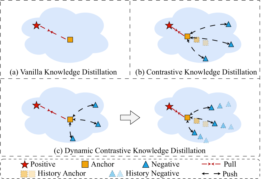
Figure 1: Difference between our DCKD and existing KD methods. (a) The Vanilla KD method overlooks the information from negative images as a lower bound. (b) Existing contrastive KD methods adopt a fixed lower bound that limits the capability of KD. (c) Our DCKD introduces dynamic contrastive regularization to perceive the student’s learning state and dynamically adjust the distilled solution space.

Knowledge distillation (KD) is an effective model compression method that transfers knowledge from a cumbersome teacher model to a lightweight student model. This process allows the student model to inherit the capabilities of the teacher model, resulting in significant performance improvements while reducing computational and storage requirements. KD has gained broad recognition for its excellent performance and broad applicability. It also can be combined with other model compression techniques, such as quantization (Du et al. 2021; Ayazoglu 2021; Hong et al. 2022), pruning (Fan et al. 2020; Wang et al. 2021a; Oh et al. 2022), compact architecture design (Ahn, Kang, and Sohn 2018; Zhang et al. 2022; Chen et al. 2022a), and neural architecture search (NAS) (Gou et al. 2020; Kim et al. 2021; He et al. 2022), to enhance the compactness of student models further.

Since KD has been well-established in natural language processing (Hahn and Choi 2019; Sanh et al. 2019; Fu et al. 2021) and high-level vision tasks (Touvron et al. 2021; Lin et al. 2022; Chen et al. 2022b), researchers have been investigating KD for image restoration methods (He et al. 2020; Lee et al. 2020; Wang et al. 2021d; Zhang et al. 2023; Li et al. 2024; Jiang et al. 2024; Zhang et al. 2024). However, these methods adopt a fixed solution space, which limits their adaptability to the evolving state of the student model during the distillation process. As illustrated in Fig. 1 (a), the vanilla distillation method (Hinton, Vinyals, and Dean 2015) only constrains the upper bound of the solution space. Although existing works (Zhang et al. 2023; Jiang et al. 2024) explore more effective and diverse upper bounds, the lack of constraints on the lower bound of the output image increases the difficulty of optimizing the solution space. This often generates low-quality images with artifacts, color distortion, and blurring. As illustrated in Fig. 1 (b), CSD (Wang et al. 2021d) introduces contrastive learning to design lower-bound constraints, significantly enhancing the transfer of knowledge from the teacher. However, in the later stages of training, the student anchor moves far from the lower bound, leading to a diminished constraint effect.

To address this problem, we propose a novel dynamic contrastive knowledge distillation framework named DCKD. Specifically, we first propose the dynamic contrastive regularization, which generates dynamic lower bound constraints. In addition, we also propose a distribution mapping module (DMM) to extract and align the pixel-level category distribution between the output of the teacher and student. Compared with previous image restoration distillation methods that primarily relied on L1 loss, DMM successfully introduces category distribution information distillation into low-level vision tasks. DCKD not only adapts to various backbones but also can be combined with methods (Zhang et al. 2023; Li et al. 2024; Jiang et al. 2024) that improve the upper bound of the solution space to further enhance distillation performance. We validate the effectiveness of DCKD across multiple image restoration tasks, including image super-resolution, deblurring, and deraining.

Overall, our main contributions are summarized as:

• We propose a dynamic contrastive distillation framework (DCKD), which can perceive the student’s learning state and dynamically optimize the lower bound of the solution space.

• We introduce a distribution mapping module to leverage category distribution information distillation, which has been significantly ignored in previous KD works for image restoration.

• Extensive experiments across various image restoration tasks demonstrate that the proposed DCKD framework significantly outperforms previous methods.

Related Work

Image Restoration

Since the pioneering works SRCNN (Dong et al. 2015) and DnCNN (Zhang et al. 2017) are firstly to employ CNNs for image restoration, various works (Lim et al. 2017; Nah, Hyun Kim, and Mu Lee 2017a; Lefkimmiatis 2017; Li et al. 2018; Ren et al. 2019; Chen et al. 2022a) have been proposed to improve the performance by increasing the parameters. Recently, Transformer-based methods (Chen et al. 2021; Liang et al. 2021; Chen et al. 2022c, 2023) have leveraged self-attention mechanisms to capture long-range dependencies, leading to significant performance improvements in image restoration. To reduce computational overhead, SAFMN (Sun et al. 2023) enhances model efficiency by utilizing spatially adaptive feature pyramid attention maps. Restormer (Zamir et al. 2022) designs channel self-attention, which is more efficient than spatial self-attention. Although lightweight designs of CNN and Transformer architectures significantly reduce computational overhead, they still face challenges regarding direct deployment on resource-constrained platforms.

Knowledge Distillation for Image Restoration

Knowledge distillation aims to significantly reduce deployment costs while improving the performance of student models by emulating the behavior of teacher models (Hinton, Vinyals, and Dean 2015; Lee et al. 2020; Gou et al. 2021). In recent years, numerous works have focused on knowledge distillation for image restoration. He et al. proposed FAKD to align the spatial affinity matrix of the feature maps between the teacher and student models (He et al. 2020). To alleviate the semantic differences between features of the teacher and student, Li et al. proposed MiPKD, which achieves feature and stochastic network block mixture in latent space (Li et al. 2024). Jiang et al. proposed MTKD that designs a composite output from multiple teachers to provide the student with a more robust teacher model (Jiang et al. 2024). However, these KD methods primarily focus on improving the upper bound of the model’s solution space, without leveraging the distribution information of the images.

Contrastive Learning for Knowledge Distillation

Recently, many researchers have explored the combination of contrastive learning and knowledge distillation to construct a comprehensive solution space (Tian, Krishnan, and Isola 2019; Xu et al. 2020; Yang et al. 2023). Wang et al. introduced contrastive learning in knowledge distillation, utilizing other images within the same dataset to construct a lower bound for the solution space (Wang et al. 2021b). Similarly, CSD (Wang et al. 2021d) proposed a contrastive self-distillation method, utilizing different images within the batch to provide lower bound constraints. Luo et al. enriched the lower bound constraints in the image deraining task by altering the direction of falling raindrops for the student model (Luo et al. 2023). However, these methods employ a fixed solution space, which leads to a weakening of the lower-bound constraint when the student anchor moves away from the lower bound in the later stages of training. Different from these methods, DCKD proposes a dynamic lower-bound constraint that progressively narrows the solution space, and can also be combined with enhanced upper-bound approaches. Additionally, DMM is proposed to extract and align the pixel-level category distribution information between the teacher and student networks.

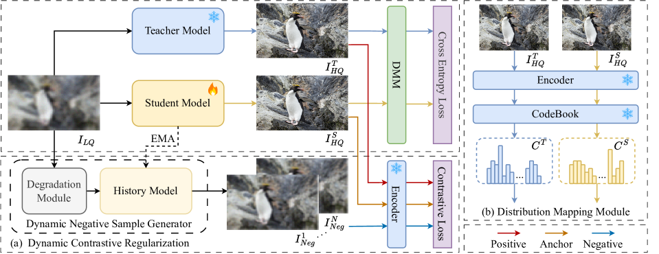
Figure 2: Illustration of the proposed Dynamic Contrastive Knowledge Distillation framework. Our DCKD consists of two parts: (a) Dynamic Contrastive Regularization (DCR), and (b) Distribution Mapping Module (DMM).

Methodology

Preliminaries

Given a low-quality image $I_{LQ}$ as input, the image restoration (IR) model $\mathcal{F}(\cdot)$ generates the corresponding high-quality image $I_{HQ}$, which can be formulated as:

$$I_{HQ}=\mathcal{F}(I_{LQ};\theta),$$ (1)

where $\theta$ represents the model parameters. The IR model $\mathcal{F}(\cdot;\theta)$ is typically optimized using the L1 norm reconstruction loss, which is defined as:

$$\mathcal{L}_{rec}=\|I_{HQ}-I_{GT}\|_{1},$$ (2)

where the $I_{GT}$ is the ground-truth image. The vanilla knowledge distillation method adds a KD loss to minimize the difference between the student model and the teacher model:

$$\mathcal{L}_{kd}=\|\mathcal{F}_{S}(I_{LQ};\theta_{s})-\mathcal{F}_{T}(I_{LQ};\theta_{t})\|_{1},$$ (3)

where $\mathcal{F}_{S}(I_{LQ};\theta_{s})$ and $\mathcal{F}_{T}(I_{LQ};\theta_{t})$ represent the outputs of student and teacher models, respectively.

Dynamic Contrastive Regularization

Previous KD methods (Hinton, Vinyals, and Dean 2015; Wang et al. 2021d) employed a fixed solution space, which causes the lower-bound constraints on the student model to weaken in the later stages of training. To address this problem, we propose dynamic contrastive regularization (DCR), which dynamically adjusts the solution space based on the student model’s state.

As shown in Fig. 2 (a), we first feed the input image $I_{LQ}$ into the dynamic negative sample generator, which consists of the degradation module and the history model. The degradation module applies random degradation operations on $I_{LQ}$, generating $N$ different degraded images $I_{dirty}$. The history model $\mathcal{F}_{S}^{his}$ then reconstructs these degraded images based on the historical state of the student model, producing $N$ different negative images $I_{Neg}$ as the lower-bound of the solution space:

$$I_{Neg}^{1},\cdots,I_{Neg}^{N}=\mathcal{F}_{S}^{his}(\mathbb{D}_{1}(I_{LQ}),\cdots,\mathbb{D}_{N}(I_{LQ})),$$ (4)

where $\mathbb{D}_{N}(\cdot)$ and $I_{Neg}^{N}$ represent the $N$-th type of random degradation and the corresponding negative image, respectively.

For the upper-bound of the solution space, we not only rely on ground-truth $I_{GT}$ to optimize the student output, as described in Eq. 2 but also consider the output of teacher model $I_{HQ}^{T}$ as the positive image $I_{Pos}$. At this point, we have defined the upper-bound and the dynamic lower-bound of the model, allowing us to construct a novel dynamic contrastive loss. We employ the pre-trained VQGAN (Esser, Rombach, and Ommer 2021) as the feature encoder. The dynamic contrastive loss is formulated as follows:

$$\mathcal{L}_{dcl}=\sum_{i=1}^{L}\lambda_{i}\frac{||f_{i}^{Anc}-f_{i}^{Pos}||_{1}}{\sum_{j=1}^{N}||f_{i}^{Anc}-f_{i,j}^{Neg}||_{1}},$$ (5)

where $f^{Anc}$, $f^{Pos}$, and $f^{Neg}$ represent the features extracted from the output of the student model, positive image and negative images, respectively. $i$ denotes the $i$-th layer of Encoder. $\lambda_{i}$ is the balancing weight for the $i$-th layer.

To better capture the state of the student model, we introduce exponential moving averages (EMA) to update the history model:

$$\theta_{his}=\alpha\theta_{his}+(1-\alpha)\theta_{stu},~{}~{}\mathrm{s.t.}~{}~{}t\%s=0,$$ (6)

where $\theta_{his}$ and $\theta_{stu}$ represent the parameters of the history model and the current student model, respectively. $\alpha$ is the attenuation rate, $t$ is the current iteration, and $s$ denotes the update step. During training, the update step $s$ gradually increases.

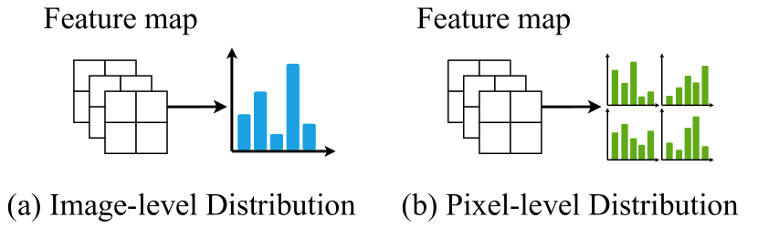
Figure 3: Illustration of the Image-level Distribution and our Pixel-level Distribution (DMM).

Distribution Mapping Module

Existing image restoration KD methods (Li et al. 2024; Jiang et al. 2024) only rely on L1-type loss to align the teacher and student models, thereby overlooking the distribution information of image content. However, high-level task KD methods (Hinton, Vinyals, and Dean 2015; Park et al. 2019; Huang et al. 2022) that align the entire output distribution of the teacher and student networks fail in low-level vision tasks. To address this, we design a distribution mapping module (DMM) to extract and align pixel-wise image distribution information, which is well-suited for pixel-level image restoration tasks.

As shown in Fig. 2 (b), we employ a pre-trained image encoder to extract deep features $F^{T}$ and $F^{S}$ from the output images of the teacher model $I_{HQ}^{T}$ and the student model $I_{HQ}^{S}$, respectively:

$$F^{T}=\operatorname{Encoder}\left(I_{HQ}^{T}\right),F^{S}=\operatorname{Encoder}\left(I_{HQ}^{S}\right).$$ (7)

We assume that high-level KD methods struggle to provide fine-grained distribution constraints, which are crucial for restoring image details. Inspired by VQGAN (Esser, Rombach, and Ommer 2021), we use the codebook $e$ pre-trained on ImageNet (Krizhevsky, Sutskever, and Hinton 2012) to obtain the pixel-wised category distribution as illustrated in Fig. 3. We also employ the corresponding VQGAN as the image encoder. The codebook further transforms the extracted deep features $F^{T}$ and $F^{S}$ into category distributions can be formulated as:

$$C^{T}=\psi(\|F^{T}-e\|_{2}^{2}),C^{S}=\psi(\|F^{S}-e\|_{2}^{2}),$$ (8)

where $C^{T}$ and $C^{S}$ represent the pixel-wised category distributions of the teacher and student models, respectively. $\psi$ denotes the softmax operation.

Finally, we use cross-entropy loss to align $C^{T}$ and $C^{S}$:

$$\mathcal{L}_{ce}=-\sum_{i=1}^{M}C_{i}^{T}\log{C_{i}^{S}},$$ (9)

where $C_{i},i=1,2,\cdots M$ is category i. $M$ is the total number of categories.

Overall Loss

Following (Hinton, Vinyals, and Dean 2015; Zhang et al. 2023; Li et al. 2024), our DCKD also compute the reconstruction loss $\mathcal{L}_{res}$ in Eq. 2 and the vanilla distillation loss $\mathcal{L}_{kd}$ in Eq. 3. In addition, the dynamic contrastive loss $\mathcal{L}_{dcl}$ in Eq. 5 and the cross-entropy loss $\mathcal{L}_{ce}$ in Eq. 9 are also accumulated. The overall loss function can be expressed as:

$$\mathcal{L}=\mathcal{L}_{rec}+\mathcal{L}_{kd}+\lambda_{dcl}\mathcal{L}_{dcl}+\lambda_{ce}\mathcal{L}_{ce},$$ (10)

where the $\lambda_{dcl}$ and $\lambda_{ce}$ are the balancing parameters. The teacher model and the encoder are frozen during the training stage.

Experiments

Experimental Settings

Teacher Backbones

The proposed DCKD is evaluated on three image restoration tasks: image super-resolution, image deblurring, and image deraining. Following (Li et al. 2024), we verify the effectiveness of DCKD on Transformer-based SwinIR (Liang et al. 2021) and CNN-based RCAN (Zhang et al. 2018) in image super-resolution. For image deblurring, we use NAFNet (Chen et al. 2022a) and Restormer (Zamir et al. 2022) as the teacher backbones. For image deraining, we employ Restormer as the backbone. The configuration details of teacher and student models are presented in Tab. 1.

Model	Role	Channel	Block/Group	#Params
SwinIR	Teacher	180	6/-	11.9M
	Student	60	4/-	1.2M
RCAN	Teacher	64	20/10	15.6M
	Student	64	6/10	5.2M
NAFNet	Teacher	32	36/-	17.1M
	Student	16	22/-	2.7M
Restormer	Teacher	48	44/-	26.1M
	Student	24	22/-	3.8M

Table 1: The specifications of teacher and student models.

Datasets and Evaluation

For image super-resolution, DCKD is trained using 800 images from DIV2K (Timofte et al. 2017) and evaluated on four benchmark datasets. For image deblurring, the models are trained and tested both on GoPro dataset (Nah, Hyun Kim, and Mu Lee 2017b). For image deraining, we train DCKD on 13,712 clean-rainy image pairs collected from multiple datasets (Fu et al. 2017; Yang et al. 2017; Zhang, Sindagi, and Patel 2019; Li et al. 2016) and evaluate it on Test100 (Zhang, Sindagi, and Patel 2019), Rain100H (Yang et al. 2017), Rain100L (Yang et al. 2017), Test2800 (Fu et al. 2017), and Test1200 (Zhang and Patel 2018). We employ the PSNR and SSIM (Wang et al. 2004) metrics to evaluate the restoration performance. For image super-resolution and image deraining tasks, the metrics are computed on the Y channel in the YCbCr color space. For image deblurring, PSNR and SSIM are evaluated in the RGB color space.

Implementation Details

For image super-resolution, the input is randomly cropped into $48\times 48$ patches and augmented by random horizontal and vertical flips and rotations. All the models are trained using ADAM optimizer (Kingma and Ba 2014) with $\beta_{1}=0.9$, $\beta_{2}=0.99$, and $\epsilon=10^{-8}$. The training batch size is set to 16 with a total of $2.5\times 10^{5}$ iterations. The initial learning rate is set to $10^{-4}$ and is decayed by a factor of 10 at every $10^{5}$ update. DCKD is implemented by PyTorch using 4 NVIDIA V100 GPUs. For other image restoration tasks, we strictly adhere to the original training configurations of each teacher model. More training configurations for other tasks are presented in the Appendix.

Scale	Method	Model	Set5	Set14	BSD100	Urban100	Model	Set5	Set14	BSD100	Urban100
			PSNR/SSIM	PSNR/SSIM	PSNR/SSIM	PSNR/SSIM		PSNR/SSIM	PSNR/SSIM	PSNR/SSIM	PSNR/SSIM
$\times$2	Teacher	SwinIR	38.36/0.9620	34.14/0.9227	32.45/0.9030	33.40/0.9394	RCAN	38.27/0.9614	34.13/0.9216	32.41/0.9027	33.34/0.9384
	Scratch		38.00/0.9607	33.56/0.9178	32.19/0.9000	32.05/0.9279		38.13/0.9610	33.78/0.9194	32.26/0.9007	32.63/0.9327
	Logits		38.04/0.9608	33.61/0.9184	32.22/0.9003	32.09/0.9282		38.17/0.9611	33.83/0.9197	32.29/0.9010	32.67/0.9329
	FAKD		38.03/0.9608	33.63/0.9182	32.21/0.9001	32.06/0.9279		38.17/0.9612	33.83/0.9199	32.29/0.9011	32.65/0.9330
	MiPKD		38.14/0.9611	33.76/0.9194	32.29/0.9011	32.46/0.9313		38.21/0.9613	33.92/0.9203	32.32/0.9015	32.83/0.9344
	DCKD		38.17/0.9613	33.85/0.9205	32.31/0.9017	32.59/0.9330		38.25/0.9615	34.01/0.9213	32.35/0.9019	32.92/0.9351
$\times$3	Teacher		34.89/0.9312	30.77/0.8503	29.37/0.8124	29.29/0.8744		34.74/0.9299	30.65/0.8482	29.32/0.8111	29.09/0.8702
	Scratch		34.41/0.9273	30.43/0.8437	29.12/0.8062	28.20/0.8537		34.61/0.9288	30.45/0.8444	29.18/0.8074	28.59/0.8610
	Logits		34.44/0.9275	30.45/0.8443	29.14/0.8066	28.23/0.8545		34.61/0.9291	30.47/0.8447	29.21/0.8080	28.62/0.8612
	FAKD		34.42/0.9273	30.42/0.8437	29.12/0.8062	28.18/0.8533		34.63/0.9290	30.51/0.8453	29.21/0.8079	28.62/0.8612
	MiPKD		34.53/0.9283	30.52/0.8456	29.19/0.8079	28.47/0.8591		34.72/0.9296	30.55/0.8458	29.25/0.8087	28.76/0.8640
	DCKD		34.59/0.9291	30.57/0.8475	29.22/0.8093	28.63/0.8633		34.74/0.9299	30.60/0.8472	29.29/0.8099	28.87/0.8662
$\times$4	Teacher		32.72/0.9021	28.94/0.7914	27.83/0.7459	27.07/0.8164		32.63/0.9002	28.87/0.7889	27.77/0.7436	26.82/0.8087
	Scratch		32.31/0.8955	28.67/0.7833	27.61/0.7379	26.15/0.7884		32.38/0.8971	28.69/0.7842	27.63/0.7379	26.36/0.7947
	Logits		32.27/0.8954	28.67/0.7833	27.62/0.7380	26.15/0.7887		32.45/0.8980	28.76/0.7860	27.67/0.7400	26.49/0.7982
	FAKD		32.22/0.8950	28.65/0.7831	27.61/0.7380	26.09/0.7870		32.46/0.8980	28.77/0.7860	27.68/0.7400	26.50/0.7980
	MiPKD		32.39/0.8971	28.76/0.7854	27.68/0.7403	26.37/0.7956		32.46/0.8982	28.77/0.7860	27.69/0.7402	26.55/0.7998
	DCKD		32.49/0.8991	28.82/0.7877	27.72/0.7422	26.53/0.8007		32.56/0.8995	28.82/0.7877	27.73/0.7423	26.69/0.8041
	$\mathrm{\textbf{DCKD}}^{*}$		32.51/0.8992	28.88/0.7890	27.74/0.7430	26.62/0.8032		32.58/0.8996	28.86/0.7885	27.74/0.7425	26.74/0.8054

Table 2: Quantitative comparison on the benchmark datasets for image super-resolution. The best and second-best performances are highlighted in bold and underlined, respectively. The FAKD results on SwinIR are from our reproduction experiments.

Model	Method	GoPro	#Params
		PSNR/SSIM
MT-RNN	-	31.15/0.9450	2.6M
DMPHN	-	31.20/0.9400	21.7M
NAFNet	Teacher	32.87/0.9606	17.1M
	Scratch	31.17/0.9457	2.7M
	Logits	31.26/0.9464	2.7M
	DCKD	31.43/0.9487	2.7M
Restormer	Teacher	32.92/0.9610	26.1M
	Scratch	31.57/0.9497	3.8M
	Logits	31.61/0.9501	3.8M
	DCKD	31.78/0.9521	3.8M

Table 3: Quantitative comparison for image deblurring.

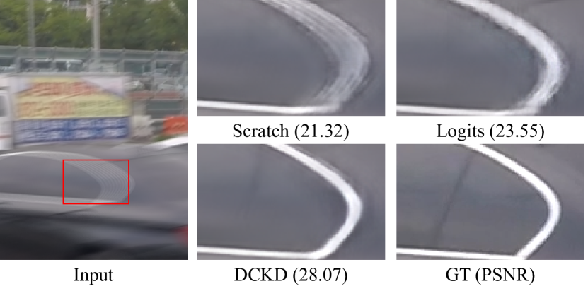
Figure 4: Visual comparison for image deblurring.

Results and Comparison

Image Super-Resolution

We compare our framework with the representative KD methods: train from scratch, Logits (Hinton, Vinyals, and Dean 2015), FAKD (He et al. 2020), and MiPKD (Li et al. 2024), on $\times 2$, $\times 3$, and $\times 4$ super-resolving scales.

The quantitative results for SwinIR and RCAN are presented in Tab. 2. Existing KD methods provide limited improvement for the student models, and in some cases, they even lead to worse performance compared to models trained without KD. For example, using FAKD for distillation on Urban100 results in worse performance than training the model from scratch on SwinIR. DCKD is effective for both Transformer-based and CNN-based architectures, significantly outperforming existing KD methods by more than 0.1dB across all three scales on Urban100. We deliberately use the most straightforward approach to demonstrate DCKD, showing that dynamic lower-bound constraints can yield strong results even without improving upper-bound constraints. To demonstrate that DCKD can be combined with methods that optimize upper-bound constraints, we incorporate DUKD (Zhang et al. 2023) into the DCKD framework to enhance upper-bound constraints, resulting in DCKD*. As we can see, the proposed DCKD can be combined with existing KD methods that optimize the upper bound, further significantly enhancing performance. DCKD* significantly outperforms the SOTA method MiPKD by 0.25dB on SwinIR and 0.19dB on RCAN at $\times 4$.

Fig. 5 and Fig. 6 present challenging visual examples for Transformer and CNN backbones, respectively. Compared to existing KD methods, our approach enables the student models to better capture structural textures, such as more accurately reconstructing sidewalk lines and building structures. More visual comparisons for various examples and models are presented in the Appendix.

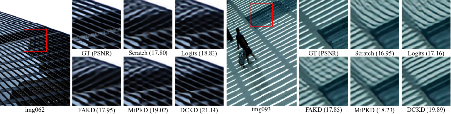
Figure 5: The visual comparison of distilling SwinIR on Urban100 for $\times 4$ SR.

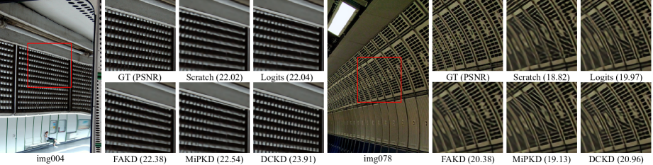
Figure 6: The visual comparison of distilling RCAN on Urban100 for $\times 4$ SR.

Model	Method	Test100	Rain100H	Rain100L	Test2800	Test1200	#Params
		PSNR/SSIM	PSNR/SSIM	PSNR/SSIM	PSNR/SSIM	PSNR/SSIM
MPRNet	-	30.27/0.8970	30.41/0.8900	36.40/0.9650	33.64/0.9380	32.91/0.9160	20.1M
SPAIR	-	30.35/0.9090	30.95/0.8920	36.93/0.9690	33.34/0.9360	33.04/0.9220	-
Restormer	Teacher	32.02/0.9237	31.48/0.9054	39.08/0.9785	34.21/0.9449	33.22/0.9270	26.1M
	Scratch	31.01/0.9122	30.51/0.8932	37.47/0.9714	33.78/0.9396	33.67/0.9295	3.8M
	Logits	31.04/0.9143	30.48/0.8915	37.17/0.9712	33.81/0.9399	33.78/0.9310	3.8M
	DCKD	31.08/0.9167	30.54/0.8969	38.02/0.9762	33.91/0.9411	33.95/0.9326	3.8M

Table 4: Quantitative comparison on the benchmark datasets for image deraining.

Image Deblurring

Tab. 3 provides a quantitative comparison on GoPro dataset. Our method demonstrates consistent effectiveness across both CNN-based NAFNet and Transformer-based Restormer. Compared to the Logits KD, our DCKD achieves 0.17dB improvement on different backbones. Moreover, with comparable parameters, the student model of NAFNet significantly outperforms MT-RNN (Park et al. 2020) by 0.28dB. Fig. 4 illustrates the deblurring visualization results. DCKD restores the clearest window outlines, significantly enhancing the deblurring capability of the student model.

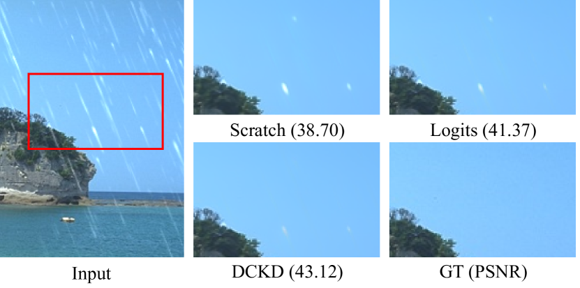
Figure 7: Visual comparison for image deraining.

Image Deraining

Tab. 4 shows the performance of various methods on several benchmark datasets for image deraining. With only 18.9% of MPRNet’s (Zamir et al. 2021) parameters, DCKD significantly surpasses it by 1.8dB on Rain100L dataset. Additionally, compared to other distillation methods, DCKD outperforms the Logits KD by 0.55dB on Rain100L. Fig. 7 provides a visual comparison of derained images. DCKD further enhances the student’s ability to remove rain streaks compared to the logits distillation method.

DCR	DMM	Set14	Urban100
		PSNR/SSIM	PSNR/SSIM
✗	✗	33.83/0.9197	32.67/0.9329
✓	✗	33.98/0.9208	32.83/0.9346
✗	✓	33.92/0.9205	32.81/0.9343
✓	✓	34.01/0.9213	32.92/0.9351

Table 5: Ablation study on components of our framework.

Degradation Type	Set14	Urban100
	PSNR/SSIM	PSNR/SSIM
Random Blur	34.01/0.9212	32.89/0.9352
Random Noise	34.01/0.9213	32.92/0.9351
Random Resize	33.99/0.9212	32.90/0.9354
Random Mix	34.00/0.9212	32.87/0.9353

Table 6: Ablation study on the degradation module.

$\lambda_{dcl}$	0.01	0.1	1.0
PSNR/SSIM	32.87/0.9346	32.92/0.9351	32.81/0.9350
$\lambda_{ce}$	0.0001	0.001	0.01
PSNR/SSIM	32.84/0.9345	32.92/0.9351	32.82/0.9341

Table 7: Ablation study on the balancing weights.

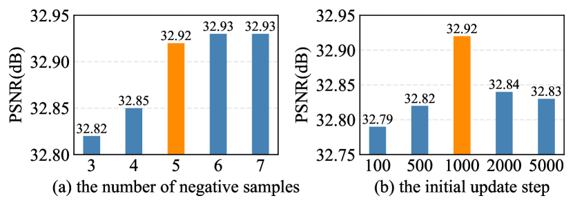
Figure 8: Ablation studies on the number of negative samples and the initial update step.

Ablation Study

For ablation experiments, we train DCKD on RCAN for the SR task with a scaling factor of $\times 2$. We then validate the results on Set14 and Urban100 datasets.

Components of the Proposed Framework

As shown in Tab. 5, we first conduct an ablation study on the two main modules of DCKD. The results indicate that our DCR and DMM outperform the baseline by 0.16dB and 0.14dB in PSNR on Urban100, respectively. This demonstrates the effectiveness of the proposed modules. Furthermore, the combination of DCR and DMM further enhances model performance, achieving PSNR improvements of 0.18dB on Set14 and 0.25dB on Urban100 compared to the baseline.

Impact of the Degradation Module

We conduct an ablation study on the impact of the degradation module in the Dynamic Negative Sample Generator (DNSG). Following Real-ESRGAN (Wang et al. 2021c), the degradation module is simple to implement by adding the Gaussian blur, Gaussian noise, resize operation (i.e., downsampling and then upsampling), or mixed degradation. The degradation results are summarized in Tab. 5 and Tab. 6. We observe that the addition degradation module (in Tab. 6) achieves at least 0.06dB PSNR improvement on Urban100, compared to that without degradation (only DMM in Tab. 5). Furthermore, the degradation with random noise achieves the highest PSNR of 32.92dB, which outperforms randomly mixed degradation by 0.05dB PSNR.

Impact of the Balancing Weights

We investigate the impact of the balancing coefficients $\lambda_{dcl}$ and $\lambda_{ce}$ in Equ. 10, as shown in Tab. 7. We find that excessively large or small values for these coefficients negatively affect the outcomes. The experiments indicate that the model achieves optimal results when $\lambda_{dcl}$ is set to 0.1 and $\lambda_{ce}$ to 0.001. Given the broad applicability of our method to various image restoration tasks, we adopt $\lambda_{dcl}=0.1$ and $\lambda_{ce}=0.001$ as the default settings across different tasks.

Impact of the Number of Negative Samples

The impact of the number of negative samples is reported in Fig. 8 (a). The results indicate that as the number of negative samples increases, the performance improves consistently. However, when the number of negative samples exceeds 5, the performance gains diminish while significantly increasing training time and memory costs. Therefore, the number of negative samples is set to 5, which achieves the best trade-off between PSNR and training time.

Impact of the Initial Update Step

In Fig. 8 (b), we investigate the impact of the initial update step for the history model within the dynamic negative sample generator. The experimental results show that when using a smaller step to update the historical model, the quality of the negative samples becomes very close to, or even surpasses, that of the anchor points, leading to instability in the solution space and a decline in performance. Conversely, when using a larger step, the negative sample quality deteriorates, weakening the lower bound constraint. When the initial update step is set to 1000 achieve the best performance.

Conclusion

In this work, we propose a dynamic contrastive knowledge distillation framework for image restoration, named DCKD, which consists of the Dynamic Contrastive Regularization (DCR) and the Distribution Mapping Module (DMM). Most previous knowledge distillation methods utilize a fixed solution space, causing the lower bound constraints to weaken gradually during training. DCR constructs a dynamic solution space based on the student’s learning state to enhance the lower-bound constraints. DMM introduces pixel-level category information to knowledge distillation for low-level vision tasks for the first time. Experiments on image super-resolution, image deblurring, and image deraining tasks validate that the proposed DCKD achieves state-of-the-art results on various benchmark datasets, both quantitatively and visually.

Model	Scale	Method	Set14	BSD100	Urban100	Manga109
			PSNR/SSIM	PSNR/SSIM	PSNR/SSIM	PSNR/SSIM
SwinIR-light	$\times$4	-	28.77/0.7858	27.69/0.7406	26.47/0.7980	30.92/0.9151
		MCLIR	28.85/0.7874	27.72/0.7414	26.57/0.8010	31.04/0.9158
		DCKD	28.88/0.7891	27.75/0.7432	26.64/0.8039	31.20/0.9180

Table 8: Quantitative comparison DCKD with MCLIR (Wu et al. 2024) on the benchmark datasets for SR task.

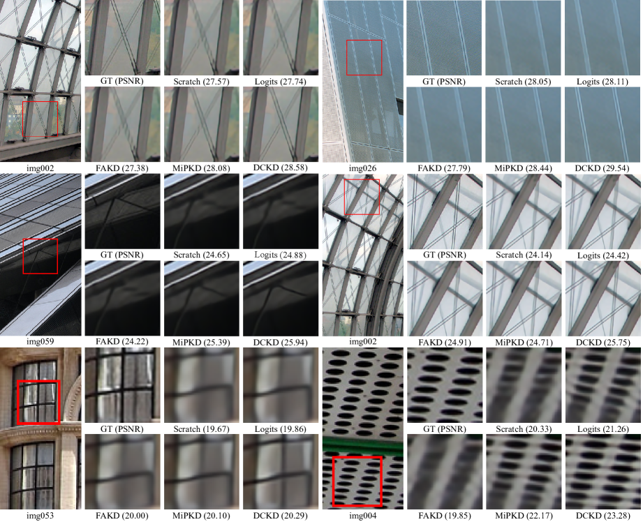
Figure 9: More visual comparison of image super-resolution at $\times 4$.

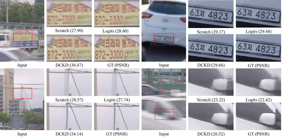
Figure 10: More visual comparison of image deblurring.

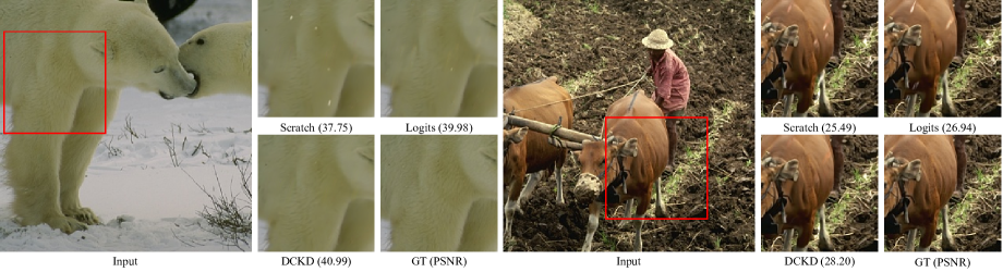
Figure 11: More visual comparison of image deraining.

Appendix

Implementation Details

The details of image encoder.

For the latent features, we extract the features from five different layers of the pre-trained VQGAN (Esser, Rombach, and Ommer 2021), while with the corresponding coefficients $\lambda_{i},i=1,\cdots 5$ to $\frac{1}{32},\frac{1}{16},\frac{1}{8},\frac{1}{4}$ and 1, respectively. We set the attenuation rate $\alpha$ to 0.1.

The details of different backbones.

For NAFNet (Chen et al. 2022a), we train the model with AdamW optimizer ($\beta_{1}=0.9$, $\beta_{2}=0.9$, weight deacy = $10^{-3}$) for total $2\times 10^{5}$ iterations with the initial learning rate $10^{-3}$ gradually reduced to $10^{-7}$ with the cosine annealing schedule (Loshchilov and Hutter 2016). The training patch size is 256 × 256 and the batch size is 32.

For Restormer (Zamir et al. 2022), we train the model with AdamW optimizer ($\beta_{1}=0.9$, $\beta_{2}=0.999$, weight deacy = $10^{-4}$) for $3\times 10^{5}$ iterations with the initial learning rate $3\times 10^{-4}$ gradually reduced to $1\times 10^{-6}$ with the cosine annealing (Loshchilov and Hutter 2016). We start training with patch size $128\times 128$ and batch size 64 for progressive learning. The patch size and batch size pairs are updated to [$(160^{2},40),(192^{2},32),(256^{2},16),(320^{2},8),(384^{2},8)$] at iterations [92K, 156K, 204K, 240K, 276K]. For data augmentation, we use horizontal and vertical flips.

Comparison of DCKD with Contrastive Learning

The quantitative comparison of DCKD with contrastive learning on the benchmark datasets for the SR task is reported in Tab. 8. DCKD significantly surpasses state-of-the-art method MCLIR (Wu et al. 2024) 0.16dB on Manga109. This shows that DCKD provides more comprehensive lower-bound constraints, ensuring that each negative sample exerts a consistent force on the anchor sample. Additionally, our method requires only a single negative sample model to generate an arbitrary number of negative samples, significantly reducing computational overhead.

More Visual Comparison

We provide more visual comparisons. Fig. 9 presents some challenging images from the x4 super-resolution task. As observed, previous distillation methods often result in blurred artifacts and a struggle to effectively restore high-frequency details such as lines and architectural structures. For example, in img002 and img026, previous methods produce significant artifacts between lines or blur the gaps between them. In contrast, our DCKD not only removes these artifacts but also clearly separates the lines. Overall, our method enhances the student model’s ability to handle high-frequency details and accurately restore them.

Further visual comparisons for deblurring and deraining tasks are shown in Fig. 10 and Fig. 11, where our DCKD effectively removes motion blur and rain, with the restored image quality closely matching that of the ground truth (GT).

References

- Ahn, Kang, and Sohn (2018) Ahn, N.; Kang, B.; and Sohn, K.-A. 2018. Fast, accurate, and lightweight super-resolution with cascading residual network. In Proceedings of the European conference on computer vision (ECCV), 252–268.
- Ayazoglu (2021) Ayazoglu, M. 2021. Extremely lightweight quantization robust real-time single-image super resolution for mobile devices. In Proceedings of the IEEE/CVF conference on computer vision and pattern recognition, 2472–2479.
- Chen et al. (2021) Chen, H.; Wang, Y.; Guo, T.; Xu, C.; Deng, Y.; Liu, Z.; Ma, S.; Xu, C.; Xu, C.; and Gao, W. 2021. Pre-trained image processing transformer. In Proceedings of the IEEE/CVF conference on computer vision and pattern recognition, 12299–12310.
- Chen et al. (2022a) Chen, L.; Chu, X.; Zhang, X.; and Sun, J. 2022a. Simple baselines for image restoration. In European conference on computer vision, 17–33. Springer.
- Chen et al. (2022b) Chen, X.; Cao, Q.; Zhong, Y.; Zhang, J.; Gao, S.; and Tao, D. 2022b. Dearkd: data-efficient early knowledge distillation for vision transformers. In Proceedings of the IEEE/CVF conference on computer vision and pattern recognition, 12052–12062.
- Chen et al. (2023) Chen, X.; Wang, X.; Zhou, J.; Qiao, Y.; and Dong, C. 2023. Activating more pixels in image super-resolution transformer. In Proceedings of the IEEE/CVF conference on computer vision and pattern recognition, 22367–22377.
- Chen et al. (2022c) Chen, Z.; Zhang, Y.; Gu, J.; Kong, L.; Yuan, X.; et al. 2022c. Cross aggregation transformer for image restoration. Advances in Neural Information Processing Systems, 35: 25478–25490.
- Dong et al. (2015) Dong, C.; Loy, C. C.; He, K.; and Tang, X. 2015. Image super-resolution using deep convolutional networks. IEEE transactions on pattern analysis and machine intelligence, 38(2): 295–307.
- Du et al. (2021) Du, Z.; Liu, J.; Tang, J.; and Wu, G. 2021. Anchor-based plain net for mobile image super-resolution. In Proceedings of the IEEE/CVF conference on computer vision and pattern recognition, 2494–2502.
- Esser, Rombach, and Ommer (2021) Esser, P.; Rombach, R.; and Ommer, B. 2021. Taming transformers for high-resolution image synthesis. In Proceedings of the IEEE/CVF conference on computer vision and pattern recognition, 12873–12883.
- Fan et al. (2020) Fan, Y.; Yu, J.; Mei, Y.; Zhang, Y.; Fu, Y.; Liu, D.; and Huang, T. S. 2020. Neural sparse representation for image restoration. Advances in Neural Information Processing Systems, 33: 15394–15404.
- Fu et al. (2021) Fu, H.; Zhou, S.; Yang, Q.; Tang, J.; Liu, G.; Liu, K.; and Li, X. 2021. LRC-BERT: latent-representation contrastive knowledge distillation for natural language understanding. In Proceedings of the AAAI Conference on Artificial Intelligence, volume 35, 12830–12838.
- Fu et al. (2017) Fu, X.; Huang, J.; Zeng, D.; Huang, Y.; Ding, X.; and Paisley, J. 2017. Removing rain from single images via a deep detail network. In Proceedings of the IEEE conference on computer vision and pattern recognition, 3855–3863.
- Gou et al. (2021) Gou, J.; Yu, B.; Maybank, S. J.; and Tao, D. 2021. Knowledge distillation: A survey. International Journal of Computer Vision, 129(6): 1789–1819.
- Gou et al. (2020) Gou, Y.; Li, B.; Liu, Z.; Yang, S.; and Peng, X. 2020. Clearer: Multi-scale neural architecture search for image restoration. Advances in neural information processing systems, 33: 17129–17140.
- Hahn and Choi (2019) Hahn, S.; and Choi, H. 2019. Self-knowledge distillation in natural language processing. arXiv preprint arXiv:1908.01851.
- He et al. (2022) He, W.; Yao, Q.; Yokoya, N.; Uezato, T.; Zhang, H.; and Zhang, L. 2022. Spectrum-aware and transferable architecture search for hyperspectral image restoration. In European Conference on Computer Vision, 19–37. Springer.
- He et al. (2020) He, Z.; Dai, T.; Lu, J.; Jiang, Y.; and Xia, S.-T. 2020. Fakd: Feature-affinity based knowledge distillation for efficient image super-resolution. In 2020 IEEE International Conference on Image Processing (ICIP), 518–522. IEEE.
- Hinton, Vinyals, and Dean (2015) Hinton, G.; Vinyals, O.; and Dean, J. 2015. Distilling the knowledge in a neural network. arXiv preprint arXiv:1503.02531.
- Hong et al. (2022) Hong, C.; Baik, S.; Kim, H.; Nah, S.; and Lee, K. M. 2022. Cadyq: Content-aware dynamic quantization for image super-resolution. In European Conference on Computer Vision, 367–383. Springer.
- Huang et al. (2022) Huang, T.; You, S.; Wang, F.; Qian, C.; and Xu, C. 2022. Knowledge distillation from a stronger teacher. Advances in Neural Information Processing Systems, 35: 33716–33727.
- Jiang et al. (2024) Jiang, Y.; Feng, C.; Zhang, F.; and Bull, D. 2024. MTKD: Multi-Teacher Knowledge Distillation for Image Super-Resolution. arXiv preprint arXiv:2404.09571.
- Kim et al. (2021) Kim, H.; Baik, S.; Choi, M.; Choi, J.; and Lee, K. M. 2021. Searching for controllable image restoration networks. In Proceedings of the IEEE/CVF International Conference on Computer Vision, 14234–14243.
- Kingma and Ba (2014) Kingma, D. P.; and Ba, J. 2014. Adam: A method for stochastic optimization. arXiv preprint arXiv:1412.6980.
- Krizhevsky, Sutskever, and Hinton (2012) Krizhevsky, A.; Sutskever, I.; and Hinton, G. E. 2012. Imagenet classification with deep convolutional neural networks. Advances in neural information processing systems, 25.
- Lee et al. (2020) Lee, W.; Lee, J.; Kim, D.; and Ham, B. 2020. Learning with privileged information for efficient image super-resolution. In Computer Vision–ECCV 2020: 16th European Conference, Glasgow, UK, August 23–28, 2020, Proceedings, Part XXIV 16, 465–482. Springer.
- Lefkimmiatis (2017) Lefkimmiatis, S. 2017. Non-local color image denoising with convolutional neural networks. In Proceedings of the IEEE conference on computer vision and pattern recognition, 3587–3596.
- Li et al. (2018) Li, C.; Guo, J.; Porikli, F.; Fu, H.; and Pang, Y. 2018. A cascaded convolutional neural network for single image dehazing. IEEE Access, 6: 24877–24887.
- Li et al. (2024) Li, S.; Zhang, Y.; Li, W.; Chen, H.; Wang, W.; Jing, B.; Lin, S.; and Hu, J. 2024. Knowledge Distillation with Multi-granularity Mixture of Priors for Image Super-Resolution. arXiv preprint arXiv:2404.02573.
- Li et al. (2016) Li, Y.; Tan, R. T.; Guo, X.; Lu, J.; and Brown, M. S. 2016. Rain streak removal using layer priors. In Proceedings of the IEEE conference on computer vision and pattern recognition, 2736–2744.
- Liang et al. (2021) Liang, J.; Cao, J.; Sun, G.; Zhang, K.; Van Gool, L.; and Timofte, R. 2021. Swinir: Image restoration using swin transformer. In Proceedings of the IEEE/CVF international conference on computer vision, 1833–1844.
- Lim et al. (2017) Lim, B.; Son, S.; Kim, H.; Nah, S.; and Mu Lee, K. 2017. Enhanced deep residual networks for single image super-resolution. In Proceedings of the IEEE conference on computer vision and pattern recognition workshops, 136–144.
- Lin et al. (2022) Lin, S.; Xie, H.; Wang, B.; Yu, K.; Chang, X.; Liang, X.; and Wang, G. 2022. Knowledge distillation via the target-aware transformer. In Proceedings of the IEEE/CVF Conference on Computer Vision and Pattern Recognition, 10915–10924.
- Loshchilov and Hutter (2016) Loshchilov, I.; and Hutter, F. 2016. Sgdr: Stochastic gradient descent with warm restarts. arXiv preprint arXiv:1608.03983.
- Luo et al. (2023) Luo, Y.; Huang, Q.; Ling, J.; Lin, K.; and Zhou, T. 2023. Local and global knowledge distillation with direction-enhanced contrastive learning for single-image deraining. Knowledge-Based Systems, 268: 110480.
- Nah, Hyun Kim, and Mu Lee (2017a) Nah, S.; Hyun Kim, T.; and Mu Lee, K. 2017a. Deep multi-scale convolutional neural network for dynamic scene deblurring. In Proceedings of the IEEE conference on computer vision and pattern recognition, 3883–3891.
- Nah, Hyun Kim, and Mu Lee (2017b) Nah, S.; Hyun Kim, T.; and Mu Lee, K. 2017b. Deep multi-scale convolutional neural network for dynamic scene deblurring. In Proceedings of the IEEE conference on computer vision and pattern recognition, 3883–3891.
- Oh et al. (2022) Oh, J.; Kim, H.; Nah, S.; Hong, C.; Choi, J.; and Lee, K. M. 2022. Attentive fine-grained structured sparsity for image restoration. In Proceedings of the IEEE/CVF Conference on Computer Vision and Pattern Recognition, 17673–17682.
- Park et al. (2020) Park, D.; Kang, D. U.; Kim, J.; and Chun, S. Y. 2020. Multi-temporal recurrent neural networks for progressive non-uniform single image deblurring with incremental temporal training. In European Conference on Computer Vision, 327–343. Springer.
- Park et al. (2019) Park, W.; Kim, D.; Lu, Y.; and Cho, M. 2019. Relational knowledge distillation. In Proceedings of the IEEE/CVF conference on computer vision and pattern recognition, 3967–3976.
- Ren et al. (2019) Ren, D.; Zuo, W.; Hu, Q.; Zhu, P.; and Meng, D. 2019. Progressive image deraining networks: A better and simpler baseline. In Proceedings of the IEEE/CVF conference on computer vision and pattern recognition, 3937–3946.
- Sanh et al. (2019) Sanh, V.; Debut, L.; Chaumond, J.; and Wolf, T. 2019. DistilBERT, a distilled version of BERT: smaller, faster, cheaper and lighter. arXiv preprint arXiv:1910.01108.
- Sun et al. (2023) Sun, L.; Dong, J.; Tang, J.; and Pan, J. 2023. Spatially-adaptive feature modulation for efficient image super-resolution. In Proceedings of the IEEE/CVF International Conference on Computer Vision, 13190–13199.
- Tian, Krishnan, and Isola (2019) Tian, Y.; Krishnan, D.; and Isola, P. 2019. Contrastive representation distillation. arXiv preprint arXiv:1910.10699.
- Timofte et al. (2017) Timofte, R.; Agustsson, E.; Van Gool, L.; Yang, M.-H.; and Zhang, L. 2017. Ntire 2017 challenge on single image super-resolution: Methods and results. In Proceedings of the IEEE conference on computer vision and pattern recognition workshops, 114–125.
- Touvron et al. (2021) Touvron, H.; Cord, M.; Douze, M.; Massa, F.; Sablayrolles, A.; and Jégou, H. 2021. Training data-efficient image transformers & distillation through attention. In International conference on machine learning, 10347–10357. PMLR.
- Wang et al. (2021a) Wang, L.; Dong, X.; Wang, Y.; Ying, X.; Lin, Z.; An, W.; and Guo, Y. 2021a. Exploring sparsity in image super-resolution for efficient inference. In Proceedings of the IEEE/CVF conference on computer vision and pattern recognition, 4917–4926.
- Wang et al. (2021b) Wang, L.; Huang, J.; Li, Y.; Xu, K.; Yang, Z.; and Yu, D. 2021b. Improving weakly supervised visual grounding by contrastive knowledge distillation. In Proceedings of the IEEE/CVF conference on computer vision and pattern recognition, 14090–14100.
- Wang et al. (2021c) Wang, X.; Xie, L.; Dong, C.; and Shan, Y. 2021c. Real-esrgan: Training real-world blind super-resolution with pure synthetic data. In Proceedings of the IEEE/CVF international conference on computer vision, 1905–1914.
- Wang et al. (2021d) Wang, Y.; Lin, S.; Qu, Y.; Wu, H.; Zhang, Z.; Xie, Y.; and Yao, A. 2021d. Towards compact single image super-resolution via contrastive self-distillation. arXiv preprint arXiv:2105.11683.
- Wang et al. (2004) Wang, Z.; Bovik, A. C.; Sheikh, H. R.; and Simoncelli, E. P. 2004. Image quality assessment: from error visibility to structural similarity. IEEE transactions on image processing, 13(4): 600–612.
- Wang et al. (2022) Wang, Z.; Cun, X.; Bao, J.; Zhou, W.; Liu, J.; and Li, H. 2022. Uformer: A general u-shaped transformer for image restoration. In Proceedings of the IEEE/CVF conference on computer vision and pattern recognition, 17683–17693.
- Wu et al. (2024) Wu, G.; Jiang, J.; Jiang, K.; and Liu, X. 2024. Learning from history: Task-agnostic model contrastive learning for image restoration. In Proceedings of the AAAI Conference on Artificial Intelligence, volume 38, 5976–5984.
- Xu et al. (2020) Xu, G.; Liu, Z.; Li, X.; and Loy, C. C. 2020. Knowledge distillation meets self-supervision. In European conference on computer vision, 588–604. Springer.
- Yang et al. (2023) Yang, C.; An, Z.; Zhou, H.; Zhuang, F.; Xu, Y.; and Zhang, Q. 2023. Online knowledge distillation via mutual contrastive learning for visual recognition. IEEE Transactions on Pattern Analysis and Machine Intelligence, 45(8): 10212–10227.
- Yang et al. (2017) Yang, W.; Tan, R. T.; Feng, J.; Liu, J.; Guo, Z.; and Yan, S. 2017. Deep joint rain detection and removal from a single image. In Proceedings of the IEEE conference on computer vision and pattern recognition, 1357–1366.
- Zamir et al. (2022) Zamir, S. W.; Arora, A.; Khan, S.; Hayat, M.; Khan, F. S.; and Yang, M.-H. 2022. Restormer: Efficient transformer for high-resolution image restoration. In Proceedings of the IEEE/CVF conference on computer vision and pattern recognition, 5728–5739.
- Zamir et al. (2021) Zamir, S. W.; Arora, A.; Khan, S.; Hayat, M.; Khan, F. S.; Yang, M.-H.; and Shao, L. 2021. Multi-stage progressive image restoration. In Proceedings of the IEEE/CVF conference on computer vision and pattern recognition, 14821–14831.
- Zhang and Patel (2018) Zhang, H.; and Patel, V. M. 2018. Density-aware single image de-raining using a multi-stream dense network. In Proceedings of the IEEE conference on computer vision and pattern recognition, 695–704.
- Zhang, Sindagi, and Patel (2019) Zhang, H.; Sindagi, V.; and Patel, V. M. 2019. Image de-raining using a conditional generative adversarial network. IEEE transactions on circuits and systems for video technology, 30(11): 3943–3956.
- Zhang et al. (2017) Zhang, K.; Zuo, W.; Chen, Y.; Meng, D.; and Zhang, L. 2017. Beyond a gaussian denoiser: Residual learning of deep cnn for image denoising. IEEE transactions on image processing, 26(7): 3142–3155.
- Zhang et al. (2024) Zhang, Q.; Liu, X.; Li, W.; Chen, H.; Liu, J.; Hu, J.; Xiong, Z.; Yuan, C.; and Wang, Y. 2024. Distilling Semantic Priors from SAM to Efficient Image Restoration Models. In Proceedings of the IEEE/CVF Conference on Computer Vision and Pattern Recognition, 25409–25419.
- Zhang et al. (2022) Zhang, X.; Zeng, H.; Guo, S.; and Zhang, L. 2022. Efficient long-range attention network for image super-resolution. In European conference on computer vision, 649–667. Springer.
- Zhang et al. (2018) Zhang, Y.; Li, K.; Li, K.; Wang, L.; Zhong, B.; and Fu, Y. 2018. Image super-resolution using very deep residual channel attention networks. In Proceedings of the European conference on computer vision (ECCV), 286–301.
- Zhang et al. (2023) Zhang, Y.; Li, W.; Li, S.; Hu, J.; Chen, H.; Wang, H.; Tu, Z.; Wang, W.; Jing, B.; and Wang, Y. 2023. Data upcycling knowledge distillation for image super-resolution. arXiv preprint arXiv:2309.14162.