Theory and numerics of subspace approximation of eigenvalue problems

Abstract

Large-scale eigenvalue problems arise in various fields of science and engineering and demand computationally efficient solutions. In this study, we investigate the subspace approximation for parametric linear eigenvalue problems, aiming to mitigate the computational burden associated with high-fidelity systems. We provide general error estimates under non-simple eigenvalue conditions, establishing the theoretical foundations for our methodology. Numerical examples, ranging from one-dimensional to three-dimensional setups, are presented to demonstrate the efficacy of reduced basis method in handling parametric variations in boundary conditions and coefficient fields to achieve significant computational savings while maintaining high accuracy, making them promising tools for practical applications in large-scale eigenvalue computations.

1 Introduction

Eigenvalue problems are of significant importance in various scientific and engineering disciplines, as they provide critical insights into the behavior and properties of complex systems. Applications range from structural dynamics, where eigenvalue analysis is used for modal analysis and vibration analysis [1], to quantum mechanics, where the Kohn-Sham equation is solved as an eigenvalue problem to determine energy levels and wave-functions [2]. In many cases, the analytical solution of such problems can not be obtained, and numerical methods can be used to approximate the solutions. However, the complexity and size of these problems can lead to significant computational demands, especially as the fidelity and resolution of models increase. It may take a long time to solve a problem even with high performance computing and efficient iterative methods such as the Locally Optimal Block Preconditioned Conjugate Gradient (LOBPCG) [3]. Consequently, reducing computational cost of eigenvalue problems without sacrificing much accuracy has become a crucial goal in scientific computing and engineering simulations.

One promising approach to achieving this goal is through reduced order modeling (ROM). Reduced order models are designed to provide efficient and accurate approximations of large-scale problems by exploiting latent representations of solution manifold and significantly reducing the dimensionality of the original problems. Low-dimensional structures can be created from compressing high-fidelity snapshot data, through linear approaches such as proper orthogonal decomposition (POD) [4], balanced truncation [5], and the reduced basis method [6], as well as nonlinear approaches like autoencoders (AE) [7, 8, 9]. Reduced systems can be formulated by projecting the large-scale systems onto low-dimensional structures. These projection-based ROM techniques integrate the reduced solution representations directly into the governing equations and numerical discretization methods, and therefore ensures that the ROMs remain grounded in the physical principles of the original problem, enhancing their accuracy and reliability while requiring less data to achieve comparable results. As a result, these approaches are both data-driven and constrained by physics, requiring less data to achieve the same level of accuracy. Moreover, to achieve meaningful speed-up, hyper-reduction techniques can be used to reduce the complexity of evaluation of the nonlinear terms in the governing equations [10, 11, 12]. Projection-based ROMs have been successfully applied to various time-dependent nonlinear problems, including the Burgers equation and Euler equations on a small scale [13, 14, 15], Navier–Stokes equations [16, 17], Lagrangian hydrodynamics [18, 19], porous media flow [20, 21], shallow water equations [22, 23], Boltzmann transport problems [24], and wave equations [25, 26, 27]. Surveys on classical projection-based ROMs can be found in [28, 29].

In contrast to the extensive research on projection-based ROMs time-dependent nonlinear problems, there is relatively less research outputs on ROMs for eigenvalue problems. Earlier works in this area include [30], who proposed a reduced-basis output bound method for symmetric eigenvalue problems. While their approach is effective for the first eigenpair, it can be restrictive in applications with non-simple eigenvalues, where multiple eigenpairs are of interest. In [31], the authors extended the reduced basis method to affinely parameterized elliptic eigenvalue problems, aiming to approximate several of the smallest eigenvalues simultaneously. The authors developed a posteriori error estimators for eigenvalues and presented various greedy strategies. In [32], the authors considered a reduced order method for approximating eigenfunctions of the Laplace problem with Dirichlet boundary conditions in a finite element setting. They used a time continuation technique to transform the problem into time-dependent and adopted a proper orthogonal decomposition (POD) approach for approximation of subsequent eigenmodes. They also presented theoretical results for choosing the optimal POD basis dimension.

In this study, we consider subspace approximation for solving parametric linear eigenvalue problems. We present a-priori error estimates of multiple eigenvalues and eigenvectors in a general setting of non-simple eigenvalues, providing rigorous theoretical foundations for the accuracy of the subspace approximation. We include several numerical examples arising from the finite element discretization of second-order elliptic differential equations, including Laplace problem, Schrödinger equation, and heterogeneous diffusion problem. These examples range from one-dimensional to three-dimensional, and incorporate various parametric boundary conditions and coefficient fields. We demonstrate the capability of reduced basis method to handle complex parametric dependencies efficiently, significantly reducing computational costs while maintaining high accuracy.

1.1 Organization

In Section 2, we describe the general setting of linear eigenvalue problems. Next, we introduce the subspace approximation in Section 3 and present an error analysis in Section 4. We provide various numerical examples of using the reduced basis methods for solving parametric linear eigenvalue problems in Section 5. Finally, a conclusion is given.

1.2 Notations

Throughout this paper, we use boldfaced lowercase letters to denote scalar vectors, and boldfaced uppercase letters to denote matrices. We also follow the following notations:

• $\mathbb{R}_{+}$ – the set of all non-negative real numbers,

• $\mathbb{R}_{++}$ – the set of all positive real numbers,

• $\mathbb{R}^{n}$ – the space of all $n$-tuple real-valued vectors,

• $\mathbb{R}^{m\times n}$ – the space of all $m\times n$ real-valued matrices,

• $\mathcal{R}(\mathbf{B})$ – the column space of a matrix $\mathbf{B}$,

• $\mathbb{S}^{n}$ – the set of all symmetric matrices in $\mathbb{R}^{n\times n}$,

• $\mathbb{S}^{n}_{++}$ – the set of all symmetric and positive definite matrices in $\mathbb{R}^{n\times n}$,

• $\text{St}(m,n)$ – the set of all orthogonal matrices in $\mathbb{R}^{m\times n}$, and

• $\text{Gr}_{m}(\mathcal{V})$ – the set of all $m$-dimensional subspaces of a vector space $\mathcal{V}$.

2 Problem statement

Suppose $\mathbf{A}\in\mathbb{S}^{n}$ is a symmetric matrix, and $\mathbf{M}\in\mathbb{S}^{n}_{++}$ is a symmetric positive definite matrix. The problem of finding the non-trivial solutions of the equation

(2.1) $$\mathbf{A}\boldsymbol{\phi}=\lambda\mathbf{M}\boldsymbol{\phi},$$

is called the generalized eigenvalue problem [33]. Under this setting, $\boldsymbol{\phi}\in\mathbb{R}^{n}\setminus\{\mathbf{0}\}$ satisfying is called a generalized eigenvector of $\mathbf{A}$ with respect to $\mathbf{M}$, and $\lambda\in\mathbb{R}$ is the associated generalized eigenvalue of $\mathbf{A}$ with respect to $\mathbf{M}$. By the spectral theorem of matrices, there exists an $\mathbf{M}$-orthonormal basis $\{\boldsymbol{\phi}_{k}\}_{k=1}^{n}\subset\mathbb{R}^{n}$ consisting of generalized eigenvectors of $\mathbf{A}$ with respect to $\mathbf{M}$, and the associated eigenvalues of $\mathbf{A}$ with respect to $\mathbf{M}$ are real and assumed to be arranged in ascending order, i.e.

(2.2) $$\lambda_{1}\leq\lambda_{2}\leq\cdots\leq\lambda_{k}\leq\lambda_{k+1}\leq\cdots\leq\lambda_{n}.$$

In a compact manner, we write the generalized eigenvalue decomposition as

(2.3) $$\mathbf{A}\boldsymbol{\Phi}=\mathbf{M}\boldsymbol{\Phi}\boldsymbol{\Lambda},$$

where $\boldsymbol{\Lambda}=\text{diag}(\lambda_{1},\lambda_{2},\cdots,\lambda_{n})$ is the diagonal matrix consisting of the generalized eigenvalues of $\mathbf{A}$ with respect to $\mathbf{M}$, and $\boldsymbol{\Phi}=\left[\boldsymbol{\phi}_{1},\boldsymbol{\phi}_{2},\cdots,\boldsymbol{\phi}_{n}\right]\in\mathbb{R}^{n\times n}$ is the matrix consisting of the generalized eigenvectors of $\mathbf{A}$ with respect to $\mathbf{M}$ satisfying $\boldsymbol{\Phi}^{\top}\mathbf{M}\boldsymbol{\Phi}=\mathbf{I}$.

Furthermore, we assume that the matrices $\mathbf{A}(\mu)$ and $\mathbf{M}(\mu)$ depend on a set of problem parameters $\mu\in\mathsf{D}$, and therefore the eigendecomposition $(\boldsymbol{\Lambda}(\mu),\boldsymbol{\Phi}(\mu))$ are also parametrized by $\mu$.

3 Subspace approximation

In this section, we present the projected eigenvalue problem onto the column space of an orthogonal matrix $\mathbf{Q}\in\text{St}(n,r)$ with $r\leq n$, which is referred to as the basis matrix. Let $\widehat{\mathbf{A}}=\mathbf{Q}^{\top}\mathbf{A}\mathbf{Q}\in\mathbb{S}^{r}$ and $\widehat{\mathbf{M}}=\mathbf{Q}^{\top}\mathbf{M}\mathbf{Q}\in\mathbb{S}_{++}^{r}$ be the projection of $\mathbf{A}$ and $\mathbf{M}$ onto the column space $\mathcal{R}(\mathbf{Q})$ of $\mathbf{Q}$ respectively. Analogously, the projected generalized eigenvalue problem is given by

(3.1) $$\widehat{\mathbf{A}}\widehat{\boldsymbol{\phi}}=\widetilde{\lambda}\widehat{\mathbf{M}}\widehat{\boldsymbol{\phi}},$$

where $\widehat{\boldsymbol{\phi}}\in\mathbb{R}^{r}\setminus\{\mathbf{0}\}$ is called a generalized eigenvector of $\widehat{\mathbf{A}}$ with respect to $\widehat{\mathbf{M}}$, and $\widetilde{\lambda}\in\mathbb{R}$ is the associated generalized eigenvalue of $\widehat{\mathbf{A}}$ with respect to $\widehat{\mathbf{M}}$. Again, by the spectral theorem of symmetric matrices, there exists an $\widehat{\mathbf{M}}$-orthonormal basis $\{\widehat{\boldsymbol{\phi}}_{k}\}_{k=1}^{r}\subset\mathbb{R}^{r}$ consisting of generalized eigenvectors of $\widehat{\mathbf{A}}$ with respect to $\widehat{\mathbf{M}}$, and the associated eigenvalues $\{\widetilde{\lambda}_{k}\}_{k=1}^{r}$ of $\widehat{\mathbf{A}}$ with respect to $\widehat{\mathbf{M}}$ are real and assumed to be arranged in ascending order, i.e.

(3.2) $$\widetilde{\lambda}_{1}\leq\widetilde{\lambda}_{2}\leq\cdots\leq\widetilde{\lambda}_{k}\leq\widetilde{\lambda}_{k+1}\leq\cdots\leq\widetilde{\lambda}_{r}.$$

The projected generalized eigenvalue decomposition can be written as

(3.3) $$\widehat{\mathbf{A}}\widehat{\boldsymbol{\Phi}}=\widehat{\mathbf{M}}\widehat{\boldsymbol{\Phi}}\widetilde{\boldsymbol{\Lambda}},$$

where $\widetilde{\boldsymbol{\Lambda}}=\text{diag}(\widetilde{\lambda}_{1},\widetilde{\lambda}_{2},\cdots,\widetilde{\lambda}_{r})$ is the diagonal matrix consisting of the generalized eigenvalues of $\widehat{\mathbf{A}}$ with respect to $\widehat{\mathbf{M}}$, and $\widehat{\boldsymbol{\Phi}}=\left[\widehat{\boldsymbol{\phi}}_{1},\widehat{\boldsymbol{\phi}}_{2},\cdots,\widehat{\boldsymbol{\phi}}_{r}\right]\in\mathbb{R}^{r\times r}$ is the matrix consisting of the generalized eigenvectors of $\widehat{\mathbf{A}}$ with respect to $\widehat{\mathbf{M}}$ satisfying $\widehat{\boldsymbol{\Phi}}^{\top}\widehat{\mathbf{M}}\widehat{\boldsymbol{\Phi}}=\mathbf{I}$. The subspace approximation of the first $r$ eigenvectors is then given by $\widetilde{\boldsymbol{\Phi}}=\mathbf{Q}\widehat{\boldsymbol{\Phi}}\in\mathbb{R}^{n\times r}$, which forms a basis for $\mathcal{R}(\mathbf{Q})$ and satisfies $\widetilde{\boldsymbol{\Phi}}^{\top}\mathbf{M}\widetilde{\boldsymbol{\Phi}}=\mathbf{I}$.

4 Analysis

In this section, we provide an error analysis for the projected eigenvalue problem (3.1), in terms of a bound on the ratio between $\lambda_{k}$ and $\widetilde{\lambda}_{k}$, and the best approximation error of $\boldsymbol{\phi}_{k}$ by the projected eigenspace of the same eigenvalue in the $\mathbf{M}$-induced norm, which is given by $\|\mathbf{x}\|_{\mathbf{M}}=\sqrt{\mathbf{x}^{\top}\mathbf{M}\mathbf{x}}$, for any $\mathbf{x}\in\mathbb{R}^{n}$. This norm is associated with the $\mathbf{M}$-induced inner product, $(\mathbf{x},\mathbf{y})\in\mathbb{R}^{n}\times\mathbb{R}^{n}\mapsto\mathbf{x}^{\top}\mathbf{M}\mathbf{y}\in\mathbb{R}$, which satisfies the Cauchy-Schwarz inequality:

(4.1) $$\mathbf{x}^{\top}\mathbf{M}\mathbf{y}\leq\|\mathbf{x}\|_{\mathbf{M}}\|\mathbf{y}\|_{\mathbf{M}}\text{ for }\mathbf{x},\mathbf{y}\in\mathbb{R}^{n}.$$

To simplify the notations of eigenpair indices, given an index set $\mathcal{S}$ with cardinality $s=|\mathcal{S}|$, we denote the matrix consisting the generalized eigenvectors of $\mathbf{A}$ with respect to $\mathbf{M}$ indexed with $\mathcal{S}$ by $\boldsymbol{\Phi}^{(\mathcal{S})}=\left[\boldsymbol{\phi}_{k}\right]_{k\in\mathcal{S}}\in\mathbb{R}^{n\times s}$. In particular, for two positive integers $m_{1}<m_{2}$, we denote the range by $\mathbb{N}(m_{1},m_{2})=\{m_{1},m_{1}+1,\cdots,m_{2}\}$, and $\boldsymbol{\Phi}^{(m_{1},m_{2})}=\boldsymbol{\Phi}^{(\mathbb{N}(m_{1},m_{2}))}$. Furthermore, for any integer $m>1$, we denote $\mathbb{N}(m)=\mathbb{N}(1,m)$ and $\boldsymbol{\Phi}^{(m)}=\boldsymbol{\Phi}^{(1,m)}$.

We start with some technical results on the generalized Rayleigh quotient with respect to $\mathbf{A}$ and $\mathbf{M}$, which is defined as: for $\mathbf{x}\in\mathbb{R}^{n}\setminus\{\mathbf{0}\}$,

(4.2) $$R_{\mathbf{A},\mathbf{M}}(\mathbf{x})=\dfrac{\mathbf{x}^{\top}\mathbf{A}\mathbf{x}}{\mathbf{x}^{\top}\mathbf{M}\mathbf{x}}.$$

Lemma 1.

Let $m_{1}<m_{2}$ be two positive integers. There hold

(4.3) $$\begin{split}\min_{\mathbf{x}\in\mathcal{R}(\boldsymbol{\Phi}^{(m_{1},m_{2})})\setminus\{\mathbf{0}\}}R_{\mathbf{A},\mathbf{M}}(\mathbf{x})&=\lambda_{m_{1}}=R_{\mathbf{A},\mathbf{M}}(\boldsymbol{\phi}_{m_{1}}),\\ \max_{\mathbf{x}\in\mathcal{R}(\boldsymbol{\Phi}^{(m_{1},m_{2})})\setminus\{\mathbf{0}\}}R_{\mathbf{A},\mathbf{M}}(\mathbf{x})&=\lambda_{m_{2}}=R_{\mathbf{A},\mathbf{M}}(\boldsymbol{\phi}_{m_{2}}).\end{split}$$

Proof.

Let $\mathbf{x}\in\mathcal{R}(\boldsymbol{\Phi}^{(m_{1},m_{2})})$. By the properties of $\mathbf{M}$-orthonormal basis,

(4.4) $$\mathbf{x}=\sum_{k=m_{1}}^{m_{2}}(\boldsymbol{\phi}_{k}^{\top}\mathbf{M}\mathbf{x})\boldsymbol{\phi}_{k}.$$

By the properties of generalized eigenvectors,

(4.5) $$\mathbf{A}\mathbf{x}=\sum_{k=m_{1}}^{m_{2}}(\lambda_{k}\boldsymbol{\phi}_{k}^{\top}\mathbf{M}\mathbf{x})\mathbf{M}\boldsymbol{\phi}_{k}.$$

Again using the properties of $\mathbf{M}$-orthonormal basis,

(4.6) $$R_{\mathbf{A},\mathbf{M}}(\mathbf{x})=\dfrac{\mathbf{x}^{\top}\mathbf{A}\mathbf{x}}{\mathbf{x}^{\top}\mathbf{M}\mathbf{x}}=\dfrac{\sum_{k=m_{1}}^{m_{2}}\lambda_{k}(\boldsymbol{\phi}_{k}^{\top}\mathbf{M}\mathbf{x})^{2}}{\sum_{k=m_{1}}^{m_{2}}(\boldsymbol{\phi}_{k}^{\top}\mathbf{M}\mathbf{x})^{2}}.$$

By the ordering of the generalized eigenvalues $\lambda_{m_{1}}\leq\lambda_{k}\leq\lambda_{m_{2}}$ for $k\in\mathbb{N}(m_{1},m_{2})$, we infer that $\lambda_{m_{1}}\leq R_{\mathbf{A},\mathbf{M}}(\mathbf{x})\leq\lambda_{m_{2}}$. ∎

The generalized eigenvalues of $\mathbf{A}$ with respect to $\mathbf{M}$ is characterized by the generalized Rayleigh quotient through the following min-max theorem.

Theorem 2 (Min-max).

For $1\leq m\leq n$, there holds

(4.7) $$\lambda_{m}=\min_{\mathcal{X}\in\text{Gr}_{m}(\mathbb{R}^{n})}\max_{\mathbf{x}\in\mathcal{X}\setminus\{\mathbf{0}\}}R_{\mathbf{A},\mathbf{M}}(\mathbf{x}).$$

Proof.

Let $\mathcal{X}\in\text{Gr}_{m}(\mathbb{R}^{n})$. By rank-nullity theorem, $\text{dim}(\mathcal{X}\cap\mathcal{R}(\boldsymbol{\Phi}^{(m-1)})^{\perp})\geq 1$. Take $\mathbf{x}_{m}\in\mathcal{X}\cap\mathcal{R}(\boldsymbol{\Phi}^{(m-1)})^{\perp}\setminus\{\mathbf{0}\}=\mathcal{X}\cap\mathcal{R}(\boldsymbol{\Phi}^{m,n})\setminus\{\mathbf{0}\}$. By Lemma 1,

(4.8) $$\lambda_{m}\leq R_{\mathbf{A},\mathbf{M}}(\mathbf{x}_{m})\leq\max_{\mathbf{x}\in\mathcal{X}\setminus\{\mathbf{0}\}}R_{\mathbf{A},\mathbf{M}}(\mathbf{x}).$$

Since $\mathcal{X}\in\text{Gr}_{m}(\mathbb{R}^{n})$ is arbitrary, we obtain

(4.9) $$\lambda_{m}\leq\inf_{\mathcal{X}\in\text{Gr}_{m}(\mathbb{R}^{n})}\max_{\mathbf{x}\in\mathcal{X}\setminus\{\mathbf{0}\}}R_{\mathbf{A},\mathbf{M}}(\mathbf{x}).$$

On the other hand, since $\mathcal{R}(\boldsymbol{\Phi}^{(m)})\in\text{Gr}_{m}(\mathbb{R}^{n})$, again by Lemma 1, we have

(4.10) $$\inf_{\mathcal{X}\in\text{Gr}_{m}(\mathbb{R}^{n})}\max_{\mathbf{x}\in\mathcal{X}\setminus\{\mathbf{0}\}}R_{\mathbf{A},\mathbf{M}}(\mathbf{x})\leq\max_{\mathbf{x}\in\mathcal{R}(\boldsymbol{\Phi}^{(m)})\setminus\{\mathbf{0}\}}R_{\mathbf{A},\mathbf{M}}(\mathbf{x})=\lambda_{m}.$$

This completes the proof. ∎

With the simplified index notations extended to $\widetilde{\boldsymbol{\Phi}}$ and $\widehat{\boldsymbol{\Phi}}$, and the definition of generalized Rayleigh-quotient extended to $(\widehat{\mathbf{A}},\widehat{\mathbf{M}})$, we have an analogous result for the approximation of generalized eigenvalues $\widetilde{\lambda}_{k}$.

Lemma 3.

Let $m_{1}<m_{2}$ be two positive integers. There hold

(4.11) $$\begin{split}\min_{\mathbf{x}\in\mathcal{R}(\widetilde{\boldsymbol{\Phi}}^{(m_{1},m_{2})})\setminus\{\mathbf{0}\}}R_{\mathbf{A},\mathbf{M}}(\mathbf{x})&=\widetilde{\lambda}_{m_{1}}=R_{\mathbf{A},\mathbf{M}}(\widetilde{\boldsymbol{\phi}}_{m_{1}}),\\ \max_{\mathbf{x}\in\mathcal{R}(\widetilde{\boldsymbol{\Phi}}^{(m_{1},m_{2})})\setminus\{\mathbf{0}\}}R_{\mathbf{A},\mathbf{M}}(\mathbf{x})&=\widetilde{\lambda}_{m_{2}}=R_{\mathbf{A},\mathbf{M}}(\widetilde{\boldsymbol{\phi}}_{m_{2}}).\end{split}$$

Proof.

Let $\mathbf{x}\in\mathcal{R}(\widetilde{\boldsymbol{\Phi}}^{(m_{1},m_{2})})\setminus\{\mathbf{0}\}$. Take $\widehat{\mathbf{x}}=\mathbf{Q}^{\top}\mathbf{x}\in\mathcal{R}(\widehat{\boldsymbol{\Phi}}^{(m_{1},m_{2})})\setminus\{\mathbf{0}\}$. Then we have $\mathbf{x}=\mathbf{Q}\widehat{\mathbf{x}}$, and

(4.12) $$R_{\mathbf{A},\mathbf{M}}(\mathbf{x})=\dfrac{(\mathbf{Q}\widehat{\mathbf{x}})^{\top}\mathbf{A}(\mathbf{Q}\widehat{\mathbf{x}})}{(\mathbf{Q}\widehat{\mathbf{x}})^{\top}\mathbf{M}(\mathbf{Q}\widehat{\mathbf{x}})}=\dfrac{\widehat{\mathbf{x}}^{\top}\widehat{\mathbf{A}}\widehat{\mathbf{x}}}{\widehat{\mathbf{x}}^{\top}\widehat{\mathbf{M}}\widehat{\mathbf{x}}}=R_{\widehat{\mathbf{A}},\widehat{\mathbf{M}}}(\widehat{\mathbf{x}}).$$

Following the proof of Lemma 1, we obtain

(4.13) $$\widetilde{\lambda}_{m_{1}}\leq R_{\widehat{\mathbf{A}},\widehat{\mathbf{M}}}(\widehat{\mathbf{x}})\leq\widetilde{\lambda}_{m_{2}}.$$

∎

In what follows, we assume $\mathbf{A}\in\mathbb{S}^{n}_{++}$ without loss of generality, or otherwise we can replace $\mathbf{A}$ by $\mathbf{A}+t\mathbf{M}$ with $t>-\lambda_{1}$. This allows us to define the $\mathbf{A}$-induced norm by $\|\mathbf{x}\|_{\mathbf{A}}=\sqrt{\mathbf{x}^{\top}\mathbf{A}\mathbf{x}}$. This norm is associated with the $\mathbf{A}$-induced inner product, $(\mathbf{x},\mathbf{y})\in\mathbb{R}^{n}\times\mathbb{R}^{n}\mapsto\mathbf{x}^{\top}\mathbf{A}\mathbf{y}\in\mathbb{R}$, which also satisfies the Cauchy-Schwarz inequality:

(4.14) $$\mathbf{x}^{\top}\mathbf{A}\mathbf{y}\leq\|\mathbf{x}\|_{\mathbf{A}}\|\mathbf{y}\|_{\mathbf{A}}\text{ for }\mathbf{x},\mathbf{y}\in\mathbb{R}^{n}.$$

To facilitate the analysis, we introduce the oblique projection onto $\mathcal{R}(\mathbf{Q})$ with the matrix $\mathbf{A}$, defined by $\mathbf{P}_{\mathbf{A}}=\mathbf{Q}\widehat{\mathbf{A}}^{-1}\mathbf{Q}^{\top}\mathbf{A}\in\mathbb{R}^{n\times n}$. The following lemma states that $\mathbf{P}_{\mathbf{A}}$ is non-expansive in the $\mathbf{A}$-induced norm.

Lemma 4.

For any $\mathbf{x}\in\mathbb{R}^{n}$, $\|\mathbf{P}_{\mathbf{A}}\mathbf{x}\|_{\mathbf{A}}\leq\|\mathbf{x}\|_{\mathbf{A}}$.

Proof.

It is straightforward to check that

(4.15) $$\mathbf{Q}^{\top}\mathbf{A}(\mathbf{I}-\mathbf{P}_{\mathbf{A}})=\mathbf{0}.$$

As a direct consequence, we have $(\mathbf{P}_{\mathbf{A}}\mathbf{x})^{\top}\mathbf{A}(\mathbf{I}-\mathbf{P}_{\mathbf{A}})\mathbf{x}=\mathbf{0}$, and hence

(4.16) $$\begin{split}\|\mathbf{P}_{\mathbf{A}}\mathbf{x}\|_{\mathbf{A}}^{2}&=(\mathbf{P}_{\mathbf{A}}\mathbf{x})^{\top}\mathbf{A}(\mathbf{P}_{\mathbf{A}}\mathbf{x})\\ &=(\mathbf{P}_{\mathbf{A}}\mathbf{x})^{\top}\mathbf{A}\mathbf{x}\\ &\leq\|\mathbf{P}_{\mathbf{A}}\mathbf{x}\|_{\mathbf{A}}\|\mathbf{x}\|_{\mathbf{A}},\end{split}$$

where we have used the Cauchy-Schwarz inequality for the $\mathbf{A}$-induced inner product. ∎

Similarly, given an index set $\mathcal{S}$, we define the oblique projection onto $\mathcal{R}(\widetilde{\boldsymbol{\Phi}}^{(\mathcal{S})})$ with the matrix $\mathbf{M}$ respectively by

(4.17) $$\widetilde{\mathbf{P}}_{\mathbf{M}}^{(\mathcal{S})}=\widetilde{\boldsymbol{\Phi}}^{(\mathcal{S})}\left[\left(\widetilde{\boldsymbol{\Phi}}^{(\mathcal{S})}\right)^{\top}\mathbf{M}\widetilde{\boldsymbol{\Phi}}^{(\mathcal{S})}\right]^{-1}\left(\widetilde{\boldsymbol{\Phi}}^{(\mathcal{S})}\right)^{\top}\mathbf{M}\in\mathbb{R}^{n\times n}.$$

The following lemma states that $\widetilde{\mathbf{P}}_{\mathbf{M}}^{(\mathcal{S})}$ maps to the best approximation in $\mathcal{R}(\widetilde{\boldsymbol{\Phi}}^{(\mathcal{S})})$ with respect to the $\mathbf{M}$-induced norm.

Lemma 5.

For any $\mathbf{x}\in\mathbb{R}^{n}$, $\|(\mathbf{I}-\widetilde{\mathbf{P}}_{\mathbf{M}}^{(\mathcal{S})})\mathbf{x}\|_{\mathbf{M}}=\min_{\mathbf{y}\in\mathcal{R}(\widetilde{\boldsymbol{\Phi}}^{(\mathcal{S})})}\|\mathbf{x}-\mathbf{y}\|_{\mathbf{M}}$.

Proof.

It is straightforward to check that

(4.18) $$\left(\widetilde{\mathbf{P}}_{\mathbf{M}}^{(\mathcal{S})}\right)^{\top}\mathbf{M}(\mathbf{I}-\widetilde{\mathbf{P}}_{\mathbf{M}}^{(\mathcal{S})})=\mathbf{0}.$$

As a direct consequence, for any $\mathbf{y}\in\mathcal{R}(\widetilde{\boldsymbol{\Phi}}^{(\mathcal{S})})$, we have $(\mathbf{y}-\widetilde{\mathbf{P}}_{\mathbf{M}}^{(\mathcal{S})}\mathbf{x})^{\top}\mathbf{M}(\mathbf{I}-\widetilde{\mathbf{P}}_{\mathbf{M}}^{(\mathcal{S})})\mathbf{x}=\mathbf{0}$, and therefore

(4.19) $$\begin{split}\|(\mathbf{I}-\widetilde{\mathbf{P}}_{\mathbf{M}}^{(\mathcal{S})})\mathbf{x}\|_{\mathbf{M}}^{2}&=(\mathbf{x}-\widetilde{\mathbf{P}}_{\mathbf{M}}^{(\mathcal{S})}\mathbf{x})^{\top}\mathbf{M}(\mathbf{I}-\widetilde{\mathbf{P}}_{\mathbf{M}}^{(\mathcal{S})})\mathbf{x}\\ &=(\mathbf{x}-\mathbf{y})^{\top}\mathbf{M}(\mathbf{I}-\widetilde{\mathbf{P}}_{\mathbf{M}}^{(\mathcal{S})})\mathbf{x}\\ &\leq\|\mathbf{x}-\mathbf{y}\|_{\mathbf{M}}\|(\mathbf{I}-\widetilde{\mathbf{P}}_{\mathbf{M}}^{(\mathcal{S})})\mathbf{x}\|_{\mathbf{M}},\end{split}$$

where we have used the Cauchy-Schwarz inequality for the $\mathbf{M}$-induced inner product. Since $\mathbf{y}\in\mathcal{R}(\widetilde{\boldsymbol{\Phi}}^{(\mathcal{S})})$ is arbitrary, we arrive at the desired result. ∎

We are now ready to present an error analysis of the generalized eigenvalues. We assume that the matrix $\mathbf{P}_{\mathbf{A}}\boldsymbol{\Phi}^{(r)}\in\mathbb{R}^{n\times r}$ is of full rank $r$, which assure that, for $1\leq m\leq r$,

(4.20) $$\kappa_{m}=\sup_{\mathbf{y}\in\mathcal{R}(\boldsymbol{\Phi}^{(m)})}\dfrac{\|\mathbf{y}\|_{\mathbf{M}}}{\|\mathbf{P}_{\mathbf{A}}\mathbf{y}\|_{\mathbf{M}}}<\infty.$$

Theorem 6.

For $1\leq m\leq r$, there holds

(4.21) $$\lambda_{m}\leq\widetilde{\lambda}_{m}\leq\kappa_{m}^{2}\lambda_{m}.$$

Proof.

First, by Lemma 3, we note that

(4.22) $$\widetilde{\lambda}_{m}=\max_{\mathbf{x}\in\mathcal{R}(\widetilde{\Phi}_{m})\setminus\{\mathbf{0}\}}R_{\mathbf{A},\mathbf{M}}(\mathbf{x}).$$

Since $\mathcal{R}(\widetilde{\boldsymbol{\Phi}}_{m})\in\text{Gr}_{m}(\mathbb{R}^{n})$, we conclude from Theorem 2 that

(4.23) $$\widetilde{\lambda}_{m}\geq\min_{\mathcal{X}\in\text{Gr}_{m}(\mathbb{R}^{n})}\max_{\mathbf{x}\in\mathcal{X}\setminus\{\mathbf{0}\}}R_{\mathbf{A},\mathbf{M}}(\mathbf{x})=\lambda_{m}.$$

On the other hand, by rank-nullity theorem, $\text{dim}(\mathcal{R}(\mathbf{P}_{\mathbf{A}}\boldsymbol{\Phi}^{(m)})\cap\mathcal{R}(\widetilde{\boldsymbol{\Phi}}^{(m-1)})^{\perp})\geq 1$. Take $\mathbf{x}_{m}\in\mathcal{R}(\mathbf{P}_{\mathbf{A}}\boldsymbol{\Phi}^{(m)})\cap\mathcal{R}(\widetilde{\boldsymbol{\Phi}}^{(m-1)})^{\perp}\setminus\{\mathbf{0}\}=\mathcal{R}(\mathbf{P}_{\mathbf{A}}\boldsymbol{\Phi}^{(m)})\cap\mathcal{R}(\widetilde{\boldsymbol{\Phi}}^{(m,r)})\setminus\{\mathbf{0}\}$. By Lemma 3, $\widetilde{\lambda}_{m}\leq R_{\mathbf{A},\mathbf{M}}(\mathbf{x}_{m})$. Take $\mathbf{y}_{m}\in\mathcal{R}(\boldsymbol{\Phi}^{(m)})$ such that $\mathbf{x}_{m}=\mathbf{P}_{\mathbf{A}}\mathbf{y}_{m}$. By Lemma 4, we have

(4.24) $$\begin{split}R_{\mathbf{A},\mathbf{M}}(\mathbf{x}_{m})&=\dfrac{\|\mathbf{P}_{\mathbf{A}}\mathbf{y}_{m}\|_{\mathbf{A}}^{2}}{\|\mathbf{P}_{\mathbf{A}}\mathbf{y}_{m}\|_{\mathbf{M}}^{2}}\\ &\leq\dfrac{\|\mathbf{y}_{m}\|_{\mathbf{A}}^{2}}{\|\mathbf{P}_{\mathbf{A}}\mathbf{y}_{m}\|_{\mathbf{M}}^{2}}\\ &=\dfrac{\|\mathbf{y}_{m}\|_{\mathbf{M}}^{2}}{\|\mathbf{P}_{\mathbf{A}}\mathbf{y}_{m}\|_{\mathbf{M}}^{2}}R_{\mathbf{A},\mathbf{M}}(\mathbf{y}_{m})\\ &\leq\kappa_{m}^{2}R_{\mathbf{A},\mathbf{M}}(\mathbf{y}_{m}).\end{split}$$

Again, by Lemma 1, $\lambda_{m}\geq R_{\mathbf{A},\mathbf{M}}(\mathbf{y}_{m})$. This completes the proof. ∎

Next, we present an error analysis for the eigenspaces spanned by the generalized eigenvectors. Let the distinct generalized eigenvalues of $\mathbf{A}$ with respect to $\mathbf{M}$ be arranged in ascending order, i.e.

(4.25) $$\nu_{1}<\nu_{2}<\cdots<\nu_{j}<\nu_{j+1}<\cdots<\nu_{p},$$

and $\gamma_{j}$ be the geometric multiplicity of $\nu_{j}$ for $1\leq j\leq p$. To classify the index in (2.2) into eigenspaces, we denote $\Gamma_{0}=0$ and $\Gamma_{j}=\sum_{i=1}^{j}\gamma_{i}$ for $1\leq j\leq p$. Then $\Gamma_{p}=n$. For $1\leq j\leq p$, we denote $\mathcal{S}_{j}=\mathbb{N}(\Gamma_{j-1}+1,\Gamma_{j})$, which implies $\lambda_{k}=\nu_{j}$ for $k\in\mathcal{S}_{j}$, and the generalized eigenspace associated with $\nu_{j}$ is given by

(4.26) $$\mathcal{E}_{j}=\mathcal{R}(\boldsymbol{\Phi}^{(\mathcal{S}_{j})})=\{\mathbf{x}\in\mathbf{R}^{n}\setminus\{0\}:\mathbf{A}\mathbf{x}=\nu_{j}\mathbf{M}\mathbf{x}\}.$$

We also denote the complement of $\mathcal{S}_{j}$ in $\mathbb{N}(r)$ by $\mathcal{S}_{j}^{\text{c}}=\mathbb{N}(r)\setminus\mathcal{S}_{j}$. We assume that for $k\in\mathcal{S}_{j}^{\text{c}}$, $\nu_{j}\notin[\lambda_{k},\kappa_{k}^{2}\lambda_{k}]$, which assures that $\nu_{j}\neq\widetilde{\lambda}_{k}$ thanks to Theorem 6, and hence

(4.27) $$\tau_{j}=\dfrac{\nu_{j}}{\min_{k\in\mathcal{S}_{j}^{\text{c}}}|\nu_{j}-\widetilde{\lambda}_{k}|}<\infty.$$

For simplicity, we assume that $\lambda_{r}<\lambda_{r+1}$, which implies $\Gamma_{\ell}=r$ for some $\ell\in\mathbb{N}(p)$.

Theorem 7.

For $1\leq j\leq\ell$, for any $\mathbf{x}\in\mathcal{E}_{j}$, we have

(4.28) $$\left\|\left(\mathbf{I}-\widetilde{\mathbf{P}}_{\mathbf{M}}^{\mathcal{S}_{j}}\right)\mathbf{x}\right\|_{\mathbf{M}}\leq\left(1+\tau_{j}\right)\|(\mathbf{I}-\mathbf{P}_{\mathbf{A}})\mathbf{x}\|_{\mathbf{M}}.$$

Proof.

Fix $1\leq j\leq\ell$. For any $\Gamma_{j-1}+1\leq m\leq\Gamma_{j}$ and $1\leq k\leq r$, by the properties of generalized eigenvectors, we have

(4.29) $$\widetilde{\boldsymbol{\phi}}_{k}^{\top}\mathbf{A}\boldsymbol{\phi}_{m}=\lambda_{m}\widetilde{\boldsymbol{\phi}}_{k}^{\top}\mathbf{M}\boldsymbol{\phi}_{m}=\mu_{j}\widetilde{\boldsymbol{\phi}}_{k}^{\top}\mathbf{M}\boldsymbol{\phi}_{m}.$$

On the other hand, again by the properties of generalized eigenvectors and v,

(4.30) $$\widetilde{\boldsymbol{\phi}}_{k}^{\top}\mathbf{A}\boldsymbol{\phi}_{m}=\widetilde{\boldsymbol{\phi}}_{k}^{\top}\mathbf{A}\mathbf{P}_{\mathbf{A}}\boldsymbol{\phi}_{m}\\ =\widetilde{\lambda}_{k}\widetilde{\boldsymbol{\phi}}_{k}^{\top}\mathbf{M}\mathbf{P}_{\mathbf{A}}\boldsymbol{\phi}_{m}.$$

Let $\mathbf{x}\in\mathcal{E}_{j}$. Then, for any $k\in\mathcal{S}_{j}^{\text{c}}$, we have

(4.31) $$\widetilde{\boldsymbol{\phi}}_{k}^{\top}\mathbf{M}\mathbf{P}_{\mathbf{A}}\mathbf{x}=\dfrac{\nu_{j}}{\widetilde{\lambda}_{k}-\nu_{j}}\widetilde{\boldsymbol{\phi}}_{k}^{\top}\mathbf{M}(\mathbf{I}-\mathbf{P}_{\mathbf{A}})\mathbf{x}.$$

By the properties of $\mathbf{M}$-orthonormal basis, we infer that

(4.32) $$\left\|\left(\mathbf{I}-\widetilde{\mathbf{P}}_{\mathbf{M}}^{\mathcal{S}_{j}}\right)\mathbf{P}_{\mathbf{A}}\mathbf{x}\right\|_{\mathbf{M}}^{2}\leq\tau_{j}^{2}\|(\mathbf{I}-\mathbf{P}_{\mathbf{A}})\mathbf{x}\|_{\mathbf{M}}^{2}.$$

By a triangle inequality for the $\mathbf{M}$-induced norm, we get

(4.33) $$\left\|\left(\mathbf{I}-\widetilde{\mathbf{P}}_{\mathbf{M}}^{\mathcal{S}_{j}}\mathbf{P}_{\mathbf{A}}\right)\mathbf{x}\right\|_{\mathbf{M}}\leq(1+\tau_{j})\left\|\left(\mathbf{I}-\mathbf{P}_{\mathbf{A}}\right)\mathbf{x}\right\|_{\mathbf{M}}.$$

Finally, we arrive at the desired result by applying Lemma 5 on $\mathcal{S}_{j}$. ∎

5 Numerical examples

In this section, we consider the finite element discretization of a general spectral problem on elliptic differential operators in an open and bounded domain $\Omega\subset\mathbb{R}^{d}$:

(5.1) $$\begin{split}-\text{div}(\sigma(x;\mu)\nabla\phi(x))+\rho(x;\mu)\phi(x)&=\lambda\phi(x)\text{ for all }x\in\Omega,\\ \alpha(x;\mu)\phi(x)+\beta(x;\mu)\mathbf{n}\cdot\nabla\phi(x)&=0\text{ for all }x\in\partial\Omega.\end{split}$$

Here $\mu\in\textsf{D}$ is a physical parameter for parametrizing the coefficient fields, including the conductivity $\sigma:\Omega\to\mathbb{R}_{++}$, the potential $\rho:\Omega\to\mathbb{R}_{+}$, and the boundary coefficients $\alpha,\beta:\partial\Omega\to\mathbb{R}_{+}$. It is assumed that $\alpha(x)>0$ or $\beta(x)>0$ for $x\in\partial\Omega$, and we denote $\Gamma_{D}=\{x\in\partial\Omega:\beta(x)=0\}$.

Let $\mathcal{V}_{h}$ be a conforming finite element space for the boundary value problem, i.e.

(5.2) $$\mathcal{V}_{h}\subset\{v\in H^{1}(\Omega):v|_{\Gamma_{D}}=0\},$$

and $\{v_{i}\}_{i=1}^{n}$ be a basis for $\mathcal{V}_{h}$. The finite element discretization of (5.1) reads: find $(\lambda,\phi_{h})\in\mathbb{R}\times\mathcal{V}_{h}$ such that

(5.3) $$\int_{\Omega}\left(a\nabla\phi_{h}\cdot\nabla v+q\phi_{h}v\right)\,\text{d}x+\int_{\partial\Omega\setminus\Gamma_{D}}\dfrac{\alpha}{\beta}\phi_{h}v\,\text{d}s=\lambda\int_{\Omega}\phi_{h}v\,\text{d}x,\text{ for all }v\in\mathcal{V}_{h},$$

which translates to the algebraic problem (2.1) with $\boldsymbol{\phi}\in\mathbb{R}^{n}$ being the coefficients of $\phi_{h}$ with respect to $\{v_{i}\}_{i=1}^{n}$, and

(5.4) $$\begin{split}\mathbf{A}_{ij}&=\int_{\Omega}\left(a\nabla v_{i}\cdot\nabla v_{j}+qv_{i}v_{j}\right)\,\text{d}x+\int_{\partial\Omega\setminus\Gamma_{D}}\dfrac{\alpha}{\beta}v_{i}v_{j}\,\text{d}s,\\ \mathbf{M}_{ij}&=\int_{\Omega}v_{i}v_{j}\,\text{d}x.\end{split}$$

We refer to the resultant eigenvalue problem (2.1) as full order model (FOM).

For each example, the basis matrix $\mathbf{Q}$ will be constructed from corresponding sample snapshot data on a set of sample parameters $\textsf{D}_{\text{train}}=\{\mu_{\ell}\}_{\ell=1}^{s}\subset\textsf{D}$. More precisely, the eigenvectors $\{\boldsymbol{\phi}_{k}(\mu_{\ell})\}_{k=1}^{p}$ are computed for $1\leq\ell\leq s$, and assembled to form a snapshot matrix of size $n\times r$, where $r=ps$. The basis matrix $\mathbf{Q}$ can be obtained from QR factorization of the snapshot matrix, and is used to formulate the projected system (3.1) at generic parameters $\mu\in\textsf{D}$. We refer to the projected eigenvalue problem (3.1) as reduced order model (ROM). We evaluate the accuracy of the ROM approximation by the following metrics:

• the error in the $k$-th eigenvalue, defined as $\widetilde{\lambda}_{k}-\lambda_{k}$, and

• the error in the $k$-th eigenvector, defined as $\left\|\left(\mathbf{I}-\widetilde{\mathbf{P}}_{\mathbf{M}}^{\mathcal{S}_{j}}\right)\boldsymbol{\phi}_{k}\right\|_{\mathbf{M}}$, where $\nu_{j}=\lambda_{k}$.

In the first two examples, the simulations are performed using MATLAB on Apple M1 Pro. In the last three examples, the simulations are performed using the finite element methods library MFEM [34] on Dane in Livermore Computing Center , on Intel Sapphire Rapids CPUs with 256 GB memory, and peak TFLOPS of 10,723.0. A visualization tool, VisIt [35], is used to visualize the coefficient and solution fields.

5.1 1D parametric boundary-value Laplacian

In this example, the computational domain is taken as the unit interval $\Omega=(0,1)\subset\mathbb{R}$, and the parameter domain is $\textsf{D}=\mathbb{R}_{+}$. For $\mu\in\textsf{D}$, the coefficient fields are given by

(5.5) $$\begin{split}\sigma(x;\mu)&=1\quad\text{for }x\in\Omega,\\ \rho(x;\mu)&=0\quad\text{for }x\in\Omega,\end{split}$$

i.e., the Laplacian operator is under consideration, and the boundary conditions are taken as

(5.6) $$\begin{split}\alpha(0;\mu)=1,\quad&\beta(0;\mu)=0,\\ \alpha(1;\mu)=\mu,\quad&\beta(1;\mu)=1,\end{split}$$

i.e., the Dirichlet boundary condition is applied at $x=0$, and the Neumann and Robin boundary conditions are applied at $x=1$ for $\mu=0$ and $\mu>0$, respectively. It is a classical result that the eigenfunctions are of the form $\phi(x)=\sin(\lambda x)$, where the spectral values $\lambda$ are solutions of $\sqrt{\lambda}+\mu\tan(\sqrt{\lambda})=0$.

The domain $\Omega$ is divided into a uniform mesh of size $h=1/2000$, and $P^{1}$ Lagrange finite elements is used in the finite element discretization, which results in a system size of $n=1999$. We are interested in the first $p=5$ eigenpairs. The eigenvalue problem (2.1) is solved by the built-in function eigs in MATLAB. Figure 1 shows the first 5 eigenvalues $\{\lambda_{k}(\mu)\}_{k=1}^{5}$ of (2.1) at different parameter values $\mu\in[0,10]$, which is verified to be the 5 smallest positive approximated solutions of $\sqrt{\lambda}+\mu\tan(\sqrt{\lambda})=0$.

Fig. 1: First 5 eigenvalues at different values of $\mu$ in the example of parametric boundary value Laplacian.

The eigenvectors $\{\boldsymbol{\phi}_{k}(\mu)\}_{k=1}^{5}$ at the sample parameters $\mu\in\textsf{D}_{\text{train}}=\{1,5,9\}$ are used as snapshots to construct the basis matrix $\mathbf{Q}$ of column size $r=15$. The projected system (3.1) is solved with the built-in function eig in MATLAB. Since all eigenvalues are single, direct comparison can be made to the FOM and ROM eigenvectors of the same index. Figure 2 shows the error in the first 5 eigenvalues and eigenvectors at different parameters $\mu\in[0,10]$. It can be seen that both approximations are extremely accurate uniformly in $\mu\in[0,10]$. The error in the eigenvalues remain below $10^{-9}$, and the error in the eigenvectors remain below $10^{-10}$.

Fig. 2: Error in first 5 eigenvalues (left) and eigenvectors (right) at different values of $\mu$ in the example of parametric boundary value Laplacian.

5.2 1D parametric harmonic oscillator

In this example, the computational domain is taken as the interval $\Omega=(-20,20)\subset\mathbb{R}$, and the parameter domain is $\textsf{D}=[0,1]$. For $\mu\in\textsf{D}$, the coefficient fields are given by

(5.7) $$\sigma(x;\mu) =1 \text{for }x\in\Omega,$$

$$\rho(x;\mu) =4(x+2-4\mu)^{2} \text{for }x\in\Omega,$$

which corresponds to the Schrödinger operator with parametric harmonic oscillator potential. The potential function $\rho$ with the parameter $\mu=0$ and $\mu=1$ are depicted in Figure 3. The Neumann boundary condition is prescribed, i.e.,

(5.8) $$\alpha(x;\mu)=0,\quad\beta(x;\mu)=1,\quad\text{for }x\in\partial\Omega=\{-20,20\}.$$

This boundary condition represents a truncation of the unbounded problem on the real line, with the minimum point in the harmonic oscillator potential shifting along $[-2,2]$ as $\mu$ varies in $[0,1]$. As a result, the eigenfunctions $\phi(x)$ also shifts as $\mu$ varies in $[0,1]$. On the other hand, the spectral values are parametric-independent. It can be easily shown that $k$-th analytic spectral values of the unbounded problem on the real line is $4k-2$ [36].

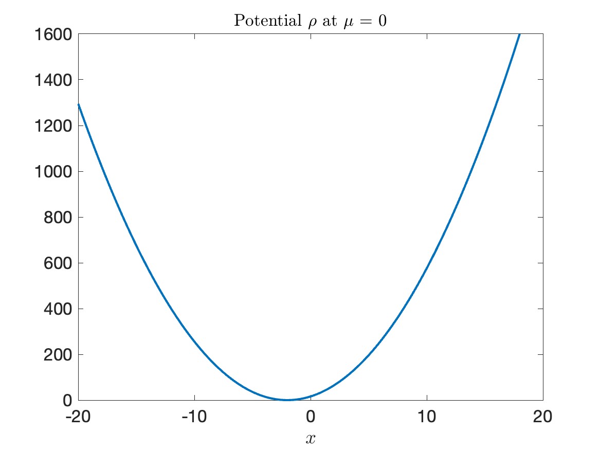
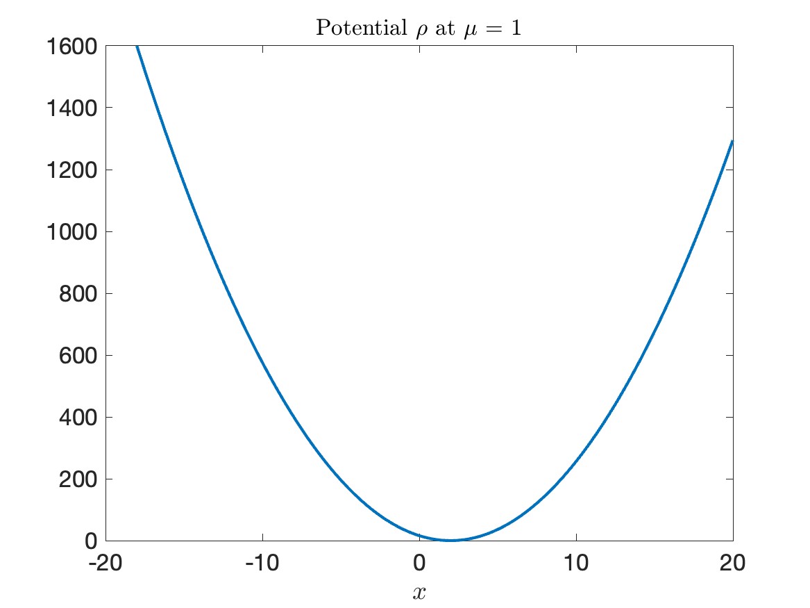
Fig. 3: Potential $\rho$ with $\mu=0$ (left) and $\mu=1$ (right) in the example of parametric harmonic oscillator.

The domain $\Omega$ is divided into a uniform mesh of size $h=1/50$, and $P^{1}$ Lagrange finite elements is used in the finite element discretization, which results in a system size of $n=2001$ We are interested in the first $p=5$ eigenpairs. The eigenvalue problem (2.1) is solved by the built-in function eigs in MATLAB. We note that the and observe that the FOM numerical approximation $\lambda_{k}(\mu)$ is always slightly larger than the analytic value, uniformly for all $\mu\in\textsf{D}$. To illustrate the difference, we compare the $k$-th eigenvalue $\lambda_{k}(\mu)$ and the corresponding analytic spectral values $4k-2$ by the logarithmic difference $\log(\lambda_{k}(\mu)-(4k-2))$ for $1\leq k\leq 5$. Figure 4 shows the first 5 eigenvalues $\{\lambda_{k}(\mu)\}_{k=1}^{5}$ of (2.1) and their logarithmic difference to the corresponding analytic spectral values at different parameter values $\mu\in[0,1]$. As the analytic spectral values of the unbounded problem are parametric-independent and the computational domain is sufficiently large, the FOM eigenvalues accurately approximate the corresponding analytic spectral values uniformly for $\mu\in[0,1]$.

Fig. 4: First 5 eigenvalues (left) and their logarithmic difference to the first 5 analytic spectral values (right) at different values of $\mu$ in the example of parametric harmonic oscillator.

The eigenvectors $\{\boldsymbol{\phi}_{k}(\mu)\}_{k=1}^{5}$ at the sample parameters $\mu\in\textsf{D}_{\text{train}}=\{0.1,0.5,0.9\}$ are used as snapshots to construct the basis matrix $\mathbf{Q}$ of column size $r=15$. The projected system (3.1) is solved with the built-in function eig in MATLAB. Since all eigenvalues are single, direct comparison can be made to the FOM and ROM eigenvectors of the same index. Figure 5 shows the error in the first 5 eigenvalues and eigenvectors at different parameters $\mu\in[0,1]$. In this example, both approximations are extremely accurate in the reproductive case, i.e. at $\mu\in\{0.1,0.5,0.9\}$, where the errors are of order $10^{-12}$. In the interpolation cases, where $\mu\in(0.1,0.9)\setminus\{0.1,0.5,0.9\}$, the errors remain below $10^{-4}$. The accuracy is the worst at the most challenging extrapolation cases $\mu\in\{0,1\}$. At $\mu=1$, the 5-th eigenvalue in the original system (2.1) is $\lambda_{5}=18.0042$, while the $5$-th eigenvalue in the projected system (3.1) is $\widetilde{\lambda}_{5}=18.1329$. The error in the $5$-th eigenvector is $1.25\times 10^{-1}$. The relatively large error in the eigenvector can be explained by the shifting behavior of the wave-functions, which makes the solution manifold has a slow decay in Kolmogorov width as seen in transport and advective phenomena [37]. Figure 6 depicts the finite element representations of the FOM solution and the ROM solution of the 5-th eigenvectors with the parameter $\mu=0$ and $\mu=1$. In spite of the relatively large error, the approximation is still reasonably accurate.

Fig. 5: Error in first 5 eigenvalues (left) and eigenvectors (right) at different values of $\mu$ in the example of parametric harmonic oscillator.

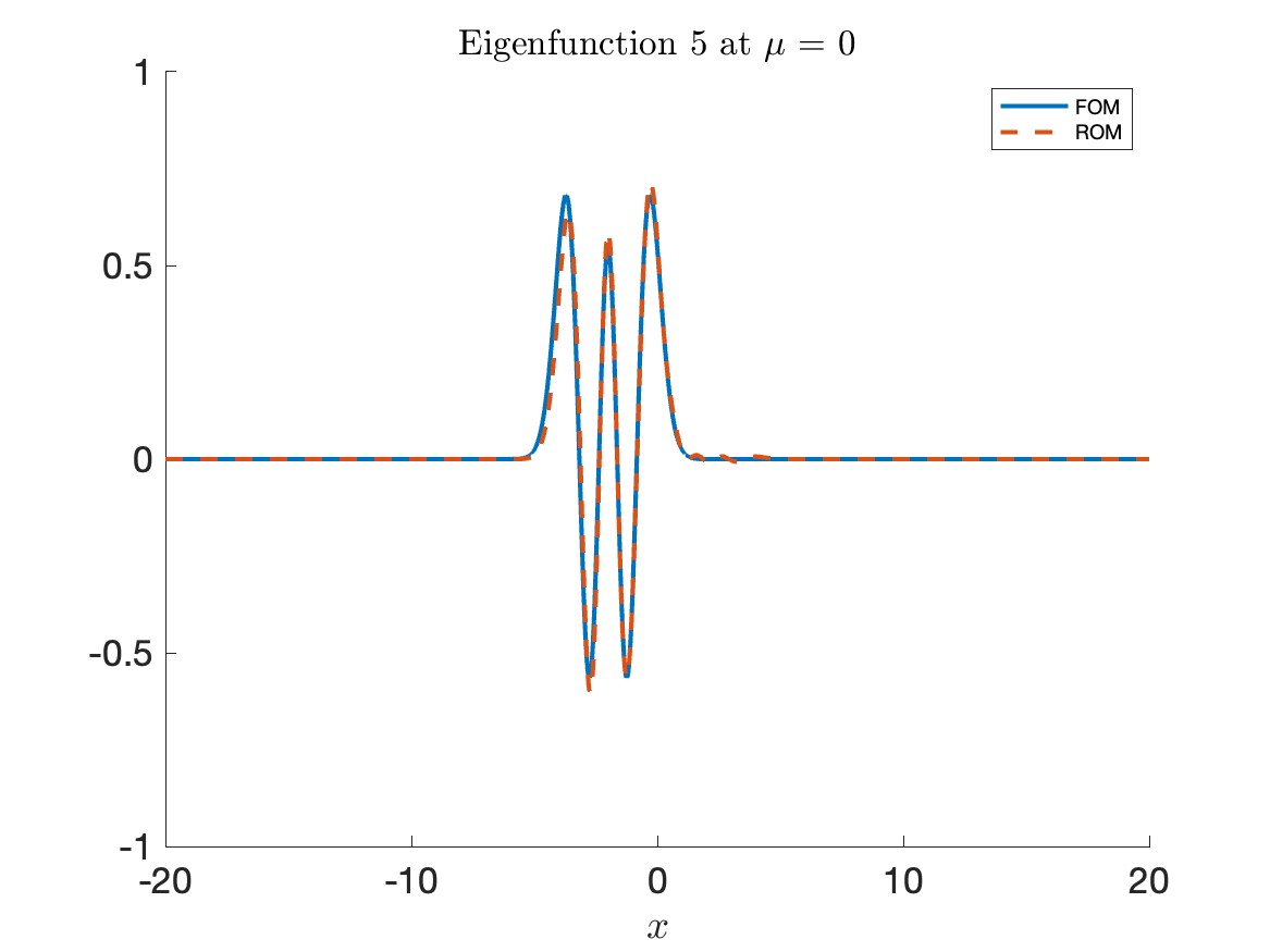
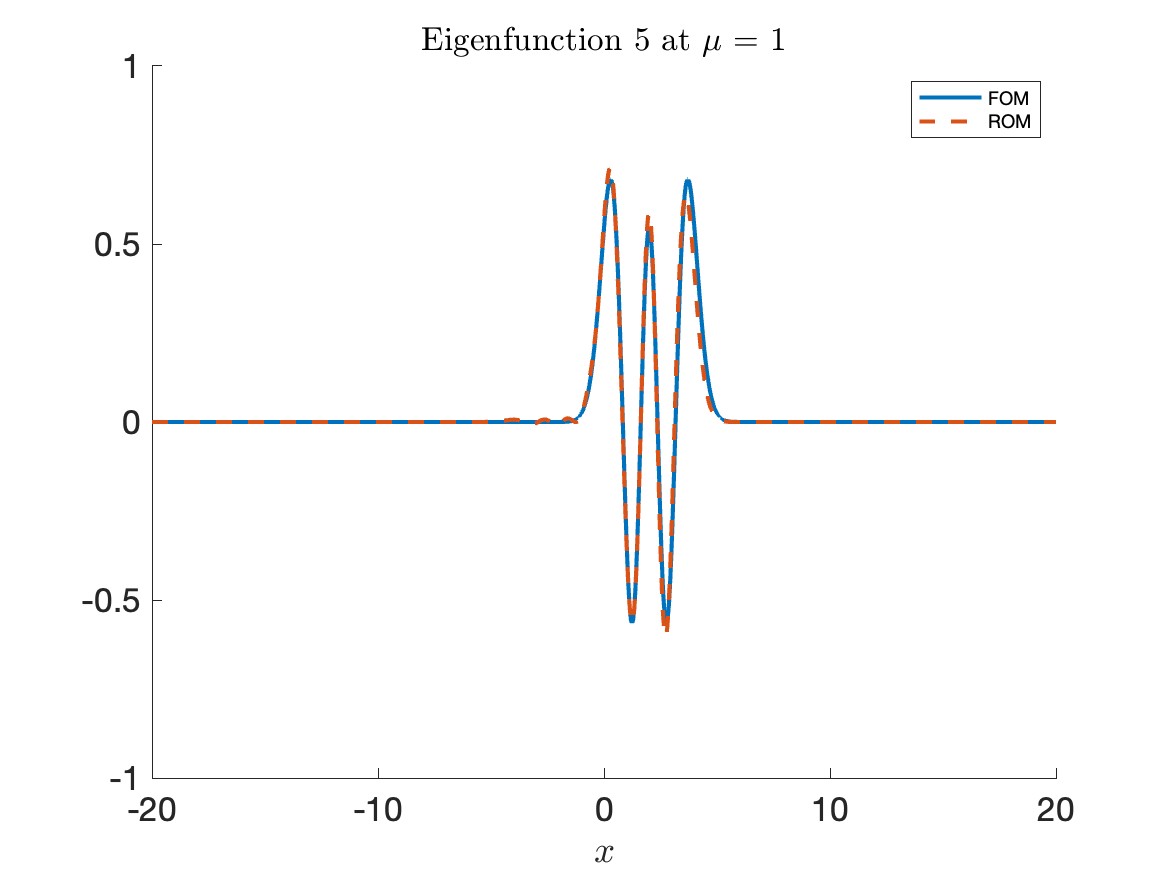
Fig. 6: Finite element representations of the FOM solution (blue solid line) and the ROM solution (red dashed line) of the 5-th eigenvectors with the parameter $\mu=0$ (left) and $\mu=1$ (right) in the example of parametric harmonic oscillator.

5.3 2D parametric Gaussian well potential

In this example, the computational domain is taken as the unit square $\Omega=(0,1)^{2}\subset\mathbb{R}^{2}$, and the parameter domain is $\textsf{D}=[-5,5]$. For $\mu\in\textsf{D}$, the coefficient fields are given by

(5.9) $$\sigma(x;\mu) =1 \text{for }x\in\Omega,$$

$$\rho(x;\mu) =-1200\exp\left(-1024(x-x_{\circ}(\mu))^{2}\right) \text{for }x\in\Omega,$$

which corresponds to the Schrödinger operator with a parametric Gaussian well potential with $x_{\circ}(\mu)=(0.5+\mu/128,0.5)$ being the center of the Gaussian well, and the Neumann boundary condition is prescribed, i.e.,

(5.10) $$\alpha(x;\mu)=0,\quad\beta(x;\mu)=1,\quad\text{for }x\in\partial\Omega.$$

Figure 7 depicts the potential coefficient $\rho$ in the domain $\Omega$ at $\mu=5$.

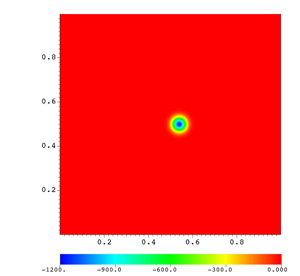
Fig. 7: Potential coefficient $\rho$ with $\mu=5$ in the example of parametric Gaussian well potential.

The domain $\Omega$ is divided into a uniform mesh of size $h=1/128$, and $Q^{1}$ Lagrange finite elements is used in the finite element discretization, which results in a system size of $n=16641$. We are interested in the first $p=1$ eigenpair, with the eigenvalue being negative. The eigenvalue problem (2.1) is solved by LOBPCG. Figure 8 shows the lowest eigenvalue $\lambda_{1}(\mu)$ of (2.1) at different parameter values $\mu\in[-5,5]$.

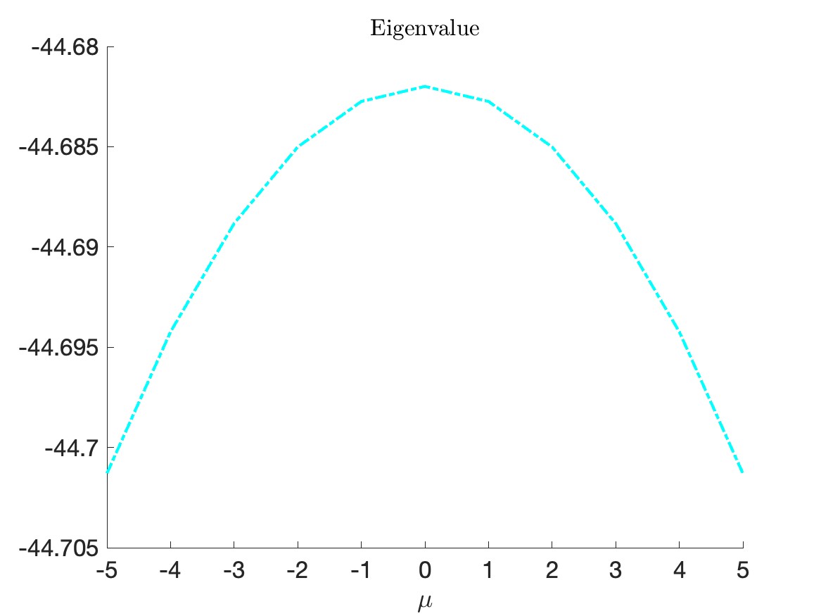
Fig. 8: Lowest eigenvalue at different values of $\mu$ in the example of parametric Gaussian well potential.

The eigenvector $\boldsymbol{\phi}_{1}(\mu)$ at the sample parameters $\mu\in\textsf{D}_{\text{train}}=\{-2.5,2.5\}$ are used as snapshots to construct the basis matrix $\mathbf{Q}$ of column size $r=2$. The projected system (3.1) is solved with the routine dsygv in LAPACK. Figure 9 shows the error in the first eigenvalue and eigenvector at different parameters $\mu\in[-5,5]$. At the interpolation case $\mu=0$, the first eigenvalue in the original system (2.1) is $\lambda_{1}=-44.6820$, while the first eigenvalue in the projected system (3.1) is $\widetilde{\lambda}_{1}=-42.4466$. The error in the first eigenvector is $3.34\times 10^{-2}$. Again, the shifting behavior of the wave-functions result in the degeneration of the accuracy in extrapolation cases. At $\mu=5$, the first eigenvalue in the original system (2.1) is $\lambda_{1}=-44.7012$, while the first eigenvalue in the projected system (3.1) is $\widetilde{\lambda}_{1}=-32.1212$. The error in the first eigenvector is $1.00\times 10^{-1}$. Figure 10 depicts the finite element representations of the FOM solution and the ROM solution of the first eigenvector with the parameter $\mu=5$. It can be seen that the peak of the ROM solution has the peak shifted to the left due to the snapshots sampled, and the decay of the ROM solution becomes asymmetric.

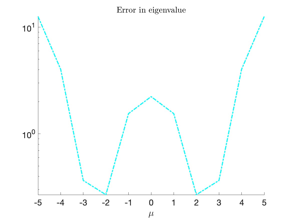
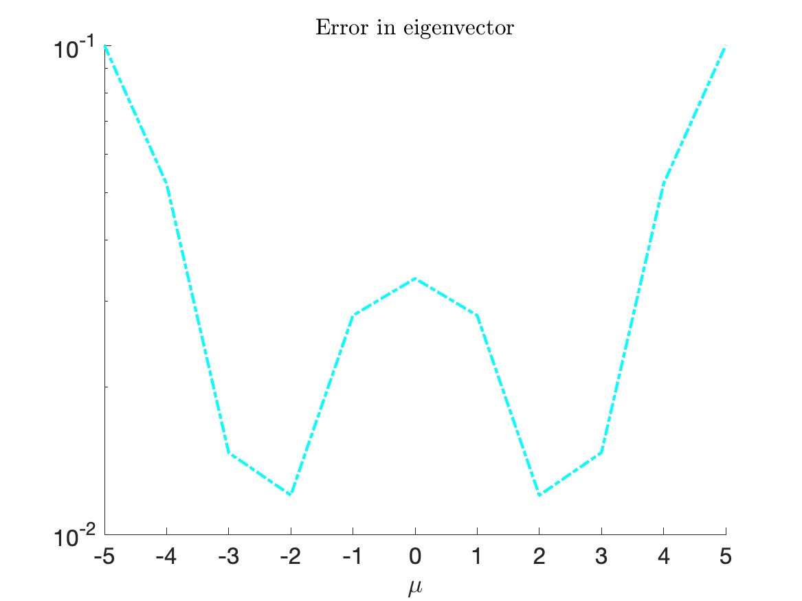
Fig. 9: Error in lowest eigenvalue (left) and eigenvector (right) at different values of $\mu$ in the example of parametric Gaussian well potential.

Fig. 10: Finite element representations of the FOM solution (left) and the ROM solution (right) of the first eigenvector with the parameter $\mu=5$ in the example of parametric Gaussian well potential.

5.4 3D parametric diatomic well potential

In this example, the computational domain is taken as the unit cube $\Omega=(0,1)^{3}\subset\mathbb{R}^{3}$, and the parameter domain is $\textsf{D}=[-2,2]$. For $\mu\in\textsf{D}$, the coefficient fields are given by

(5.11) $$\sigma(x;\mu) =1/324 \text{for }x\in\Omega,$$

$$\rho(x;\mu) =\sum_{k=1}^{2}\sum_{p=1}^{2}A_{k}\exp\left(-\dfrac{(x-x^{(p)}_{\circ}(\mu))^{2}}{2R_{k}^{2}}\right) \text{for }x\in\Omega,$$

with $A_{1}=-28.9$, $A_{2}=-3.6$, $R_{1}=7/450$, $R_{2}=3/50$, $x^{(1)}_{\circ}(\mu)=(13/36-\mu/128,1/2,1/2)$ and $x^{(2)}_{\circ}(\mu)=(23/36+\mu/128,1/2,1/2)$, which corresponds to a Kohn-Sham operator mimicking a diatomic well potential, and the Neumann boundary condition is prescribed, i.e.,

(5.12) $$\alpha(x;\mu)=0,\quad\beta(x;\mu)=1,\quad\text{for }x\in\partial\Omega.$$

The domain $\Omega$ is divided into a uniform mesh of size $h=1/128$, and $Q^{1}$ Lagrange finite elements is used in the finite element discretization, which results in a system size of $n=2146689$. We are interested in the first $p=2$ eigenpairs, with the eigenvalues being negative. The eigenvalue problem (2.1) is solved by LOBPCG. In this case, the first 2 eigenvalues are both the same with a value approximately $-4.67$, uniformly in $\mu\in[-2,2]$.

We investigate the effects of sampling for collecting the sample snapshots by comparing the results of $\textsf{D}_{\text{train}}=\{-1.25,1.25\}$ with sampling frequency 0.5, and $\textsf{D}_{\text{train}}=\{-1.25,0,1.25\}$ with sampling frequency 0.25. The eigenvectors $\{\boldsymbol{\phi}_{k}(\mu)\}_{k=1}^{2}$ at the sample parameters $\mu\in\textsf{D}_{\text{train}}$ are used as snapshots to construct the basis matrix $\mathbf{Q}$ of column size $r=4$ for $\textsf{D}_{\text{train}}=\{-1.25,1.25\}$ and $r=6$ for $\textsf{D}_{\text{train}}=\{-1.25,0,1.25\}$ respectively. The projected system (3.1) is solved with the routine dsygv in LAPACK. Figure 11 shows the error in the first eigenvalue and eigenvector at different parameters $\mu\in[0,1]$ with the sampling frequencies 0.5 and 0.25. It can be observed that using a denser sampling does not only make the approximations of the eigenvalues and eigenvectors become extremely accurate in the additional reproductive cases $\mu=0$, but also significantly increases the accuracy all the cases. At the extrapolation case $\mu=2$, the ROM approximation error of both eigenvalues is reduced from 0.09 to 0.03, and the ROM approximation error of both eigenvectors is reduced from 0.17 to 0.04. We remark that very similar results are observed for the second eigenpair.

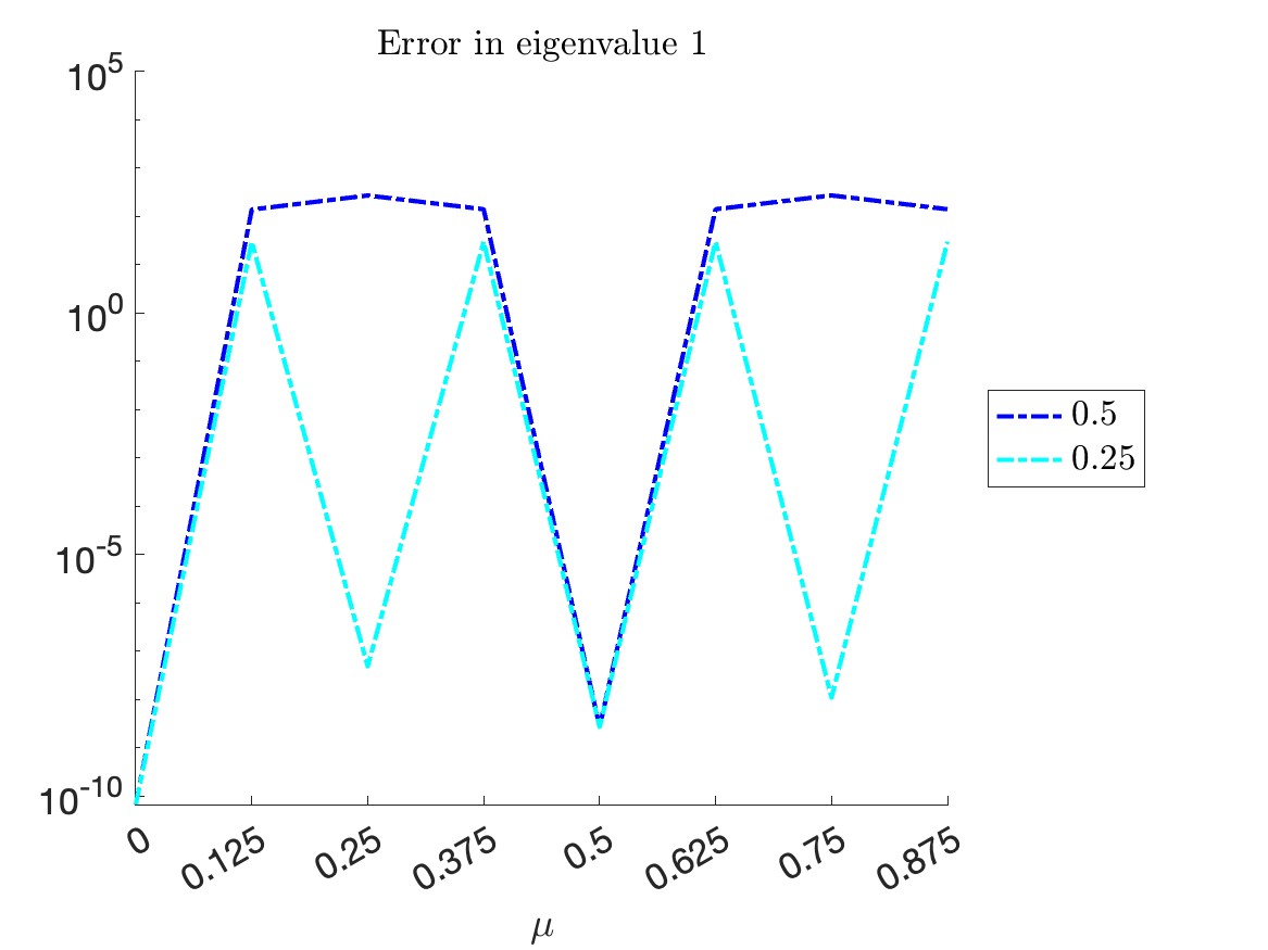
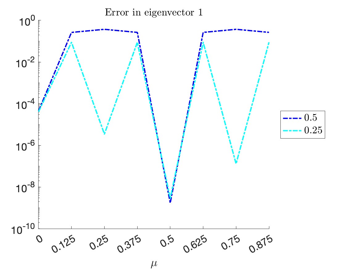
Fig. 11: Error in first eigenvalue (left) and eigenvector (right) at different values of $\mu$ with the sampling frequencies 0.5 and 0.25 in the example of parametric diatomic well potential.

5.5 3D parametric contrast heterogeneous diffusion

In this example, the computational domain is taken as the Fichera domain $\Omega=(-1,1)^{3}\setminus(-1,0]^{3}\subset\mathbb{R}^{3}$, and the parameter domain is $\textsf{D}=\mathbb{R}_{+}$. For $\mu\in\textsf{D}$, the coefficient fields are given by

(5.13) $$\sigma(x;\mu) =1+\mu\chi_{B}(x) \text{for }x\in\Omega,$$

$$\rho(x;\mu) =0 \text{for }x\in\Omega,$$

which corresponds to a heterogeneous diffusion operator with parametric contrast between the box $B=\{x\in\Omega:|x|_{\infty}\leq 0.25\}$ and the background $\Omega\setminus B$, and the Dirichlet boundary condition is prescribed, i.e.,

(5.14) $$\alpha(x;\mu)=1,\quad\beta(x;\mu)=0,\quad\text{for }x\in\partial\Omega.$$

Figure 12 depicts the conductivity coefficient $\sigma$ in the domain $\Omega$ at $\mu=10$.

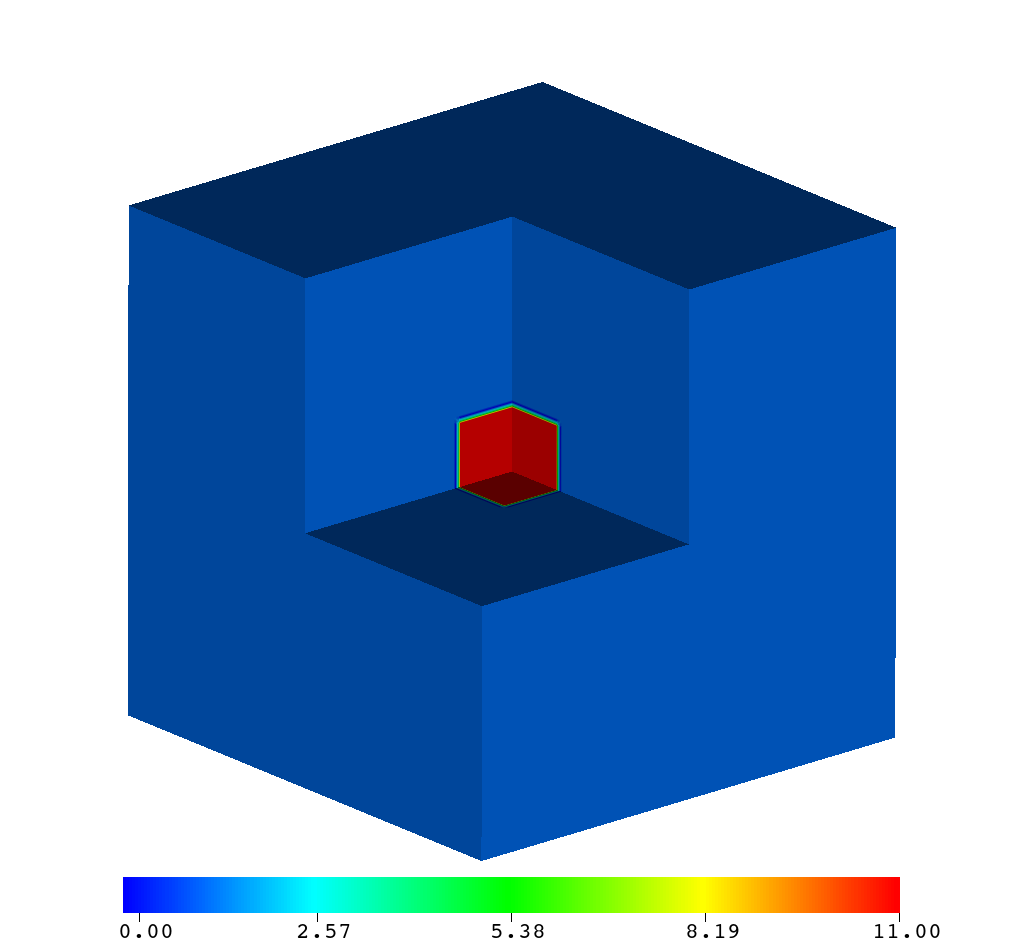
Fig. 12: Conductivity coefficient $\sigma$ with $\mu=10$ in the example of parametric contrast heterogeneous diffusion.

The domain $\Omega$ is divided into a uniform mesh of size $h=1/64$, and $Q^{2}$ Lagrange finite elements is used in the finite element discretization, which results in a system size of $n=1884545$. We are interested in the first $p=10$ eigenpairs. The eigenvalue problem (2.1) is solved by LOBPCG. Figure 13 shows the first 10 eigenvalues $\{\lambda_{k}(\mu)\}_{k=1}^{10}$ of (2.1) at different parameter values $\mu\in[0,1]$. In this case, there are 3 sets of double eigenvalue, namely $\lambda_{2}=\lambda_{3}$, $\lambda_{5}=\lambda_{6}$, and $\lambda_{8}=\lambda_{9}$, uniformly in $\mu\in[0,1]$.

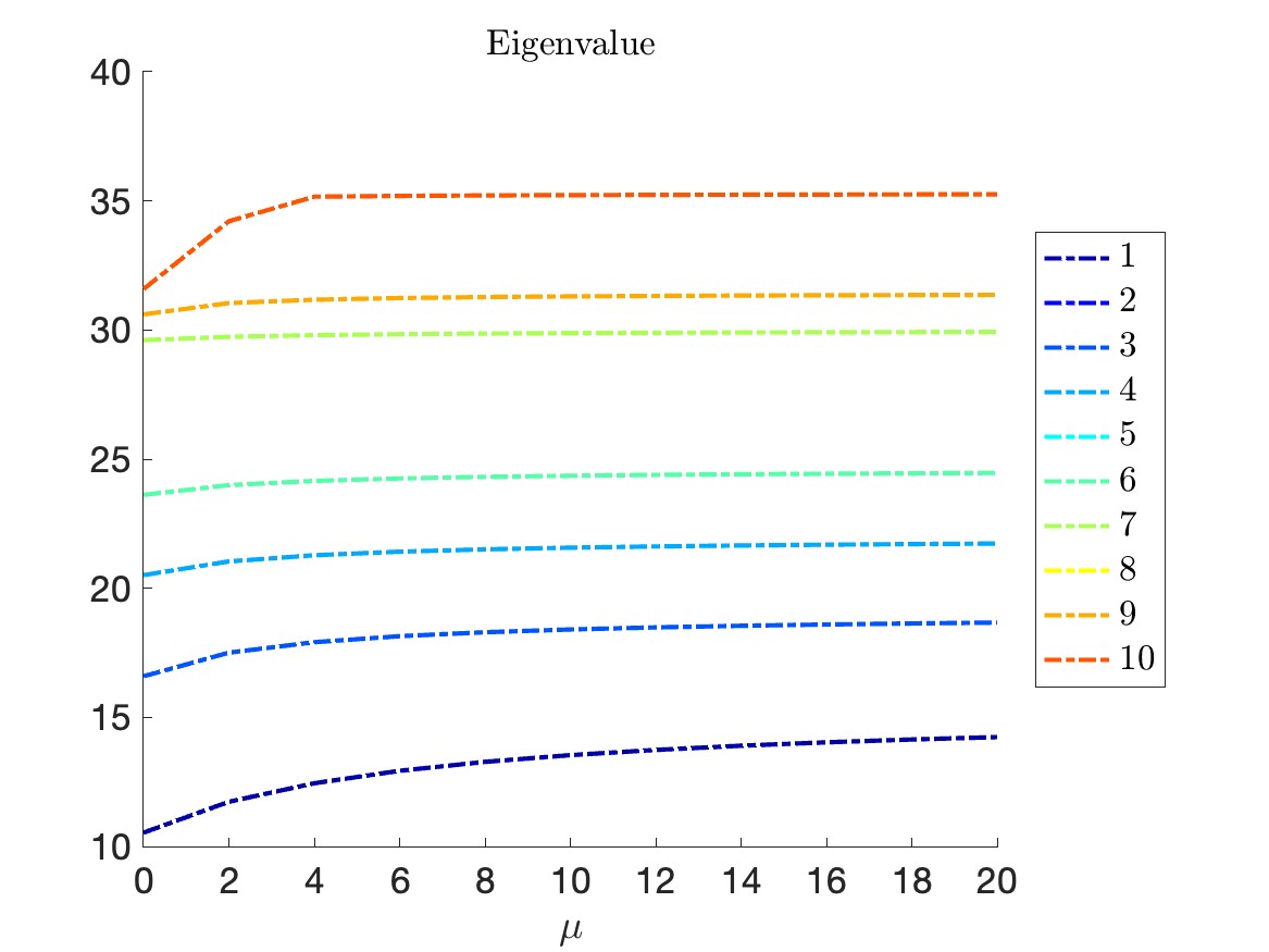
Fig. 13: First 10 eigenvalues at different values of $\mu$ in the example of parametric contrast heterogeneous diffusion.

The eigenvectors $\{\boldsymbol{\phi}_{k}(\mu)\}_{k=1}^{10}$ at the sample parameters $\mu\in\textsf{D}_{\text{train}}=\{0,10,20\}$ are used as snapshots to construct the basis matrix $\mathbf{Q}$ of column size $r=30$. The projected system (3.1) is solved with the routine dsygv in LAPACK. Due to the repeated eigenvalues, in the calculation of the error in the $k$-th eigenvector, we need to identify the subspace $\mathcal{E}_{j}$ where $\lambda_{k}=\nu_{j}$, and compute the projection $\widetilde{\mathbf{P}}_{\mathbf{M}}^{\mathcal{S}_{j}}$, which depends on the correlation matrix $\mathbf{C}\in\mathbb{R}^{10\times 10}$, defined by

(5.15) $$\mathbf{C}_{km}=\widetilde{\boldsymbol{\phi}}_{m}^{\top}\mathbf{M}\boldsymbol{\phi}_{k}.$$

The ROM approximation of the $k$-th eigenvector can be expressed as

(5.16) $$\widetilde{\mathbf{P}}_{\mathbf{M}}^{\mathcal{S}_{j}}\boldsymbol{\phi}_{k}=\sum_{m:\lambda_{m}=\lambda_{k}}\mathbf{C}_{km}\widetilde{\boldsymbol{\phi}}_{m}.$$

Figure 14 shows all the entries of the correlation matrix $\mathbf{C}$ with $\mu=6$. The calculation of the ROM approximations of the eigenvectors only utilizes the block matrices surrounded by the red boxes, within which the indices of the eigenpairs corresponding to the same eigenspace. Moreover, it can be observed that the off-diagonal blocks are approximately zero (up to 2 decimal places), meaning the FOM solutions $\boldsymbol{\phi}_{k}$ are almost orthogonal to all the ROM approximations $\widetilde{\boldsymbol{\phi}}_{m}$ outside their own eigenspace where $\lambda_{m}\neq\lambda_{k}$. Figure 15 shows the error in the first 10 eigenvalues and eigenvectors at different parameters $\mu\in[0,20]$. Similar to the previous examples, both approximations are extremely accurate in the reproductive case, and reasonably accurate in the interpolation cases.

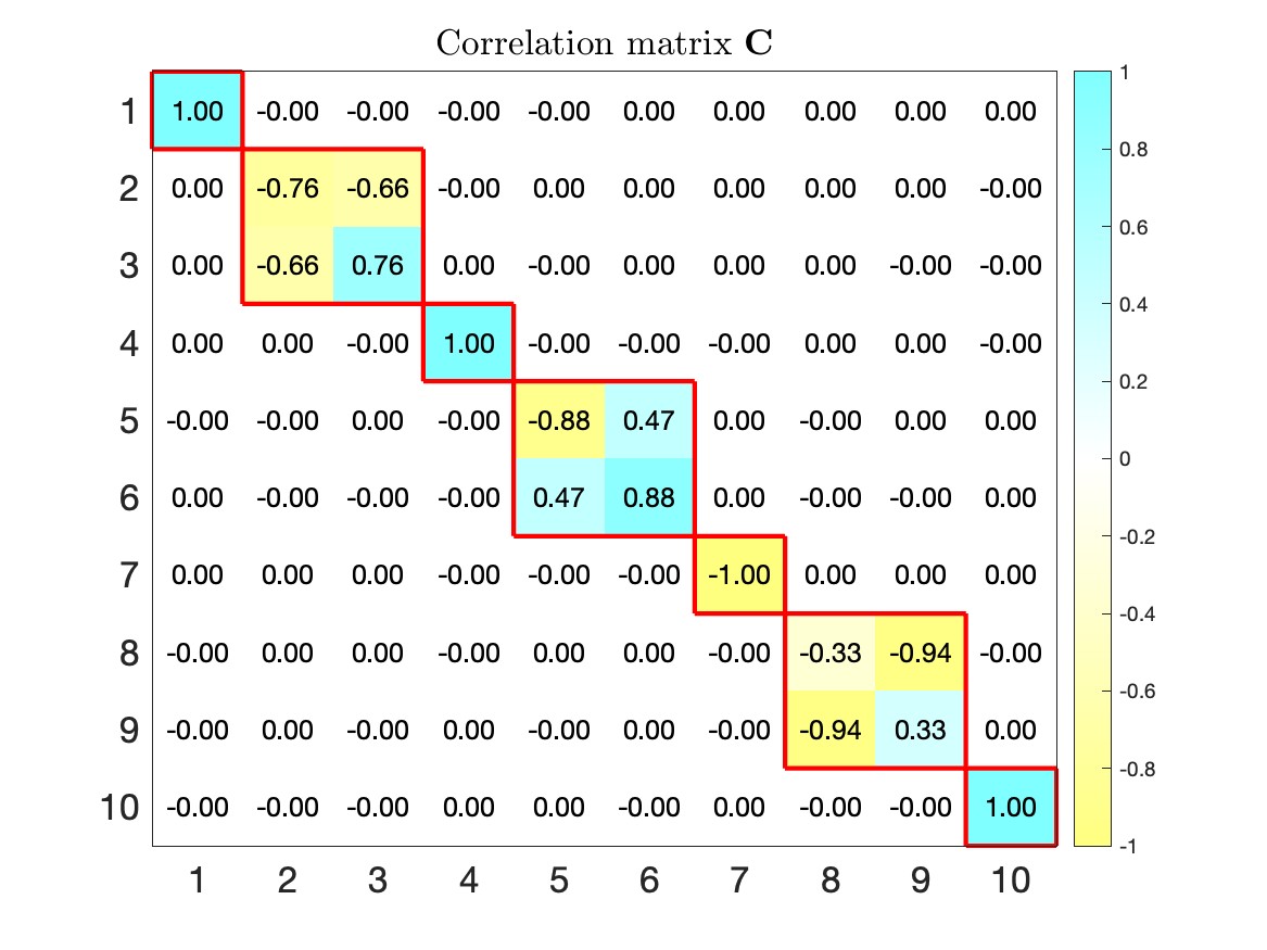
Fig. 14: Correlation matrix $\mathbf{C}$ with $\mu=6$ in the example of parametric contrast heterogeneous diffusion.

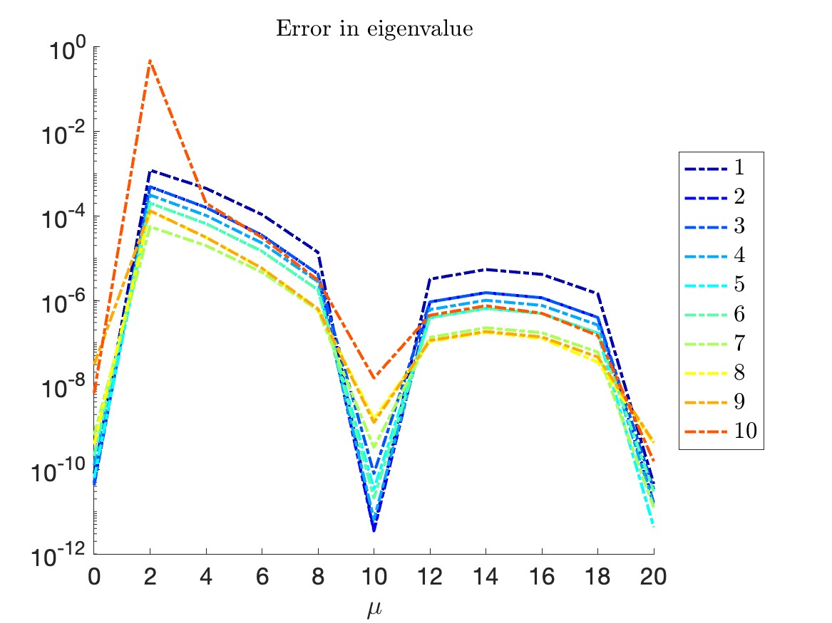
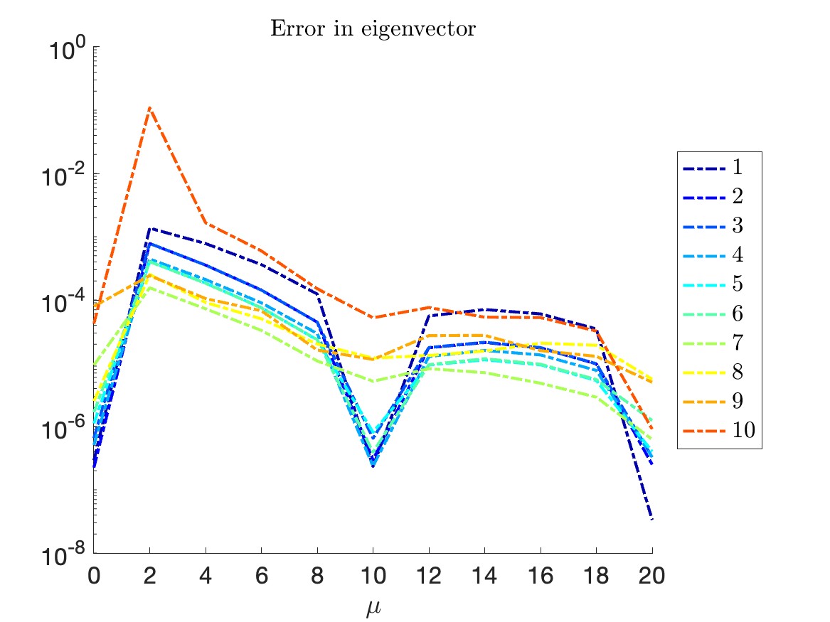
Fig. 15: Error in first 10 eigenvalues (left) and eigenvectors (right) at different values of $\mu$ in the example of parametric contrast heterogeneous diffusion.

6 Conclusion

In this paper, we presented theoretical and numerical studies of reduced basis approximation for solving parametric linear eigenvalue problems. We derived general a-priori error estimates of the eigenvalues and the eigenvectors through the min-max principles. The error bounds are controlled by several quantities, including the oblique projectors and the spectral gaps. We provided various numerical examples of finite element discretization of Laplace, Kohn-Sham, and diffusion eigenvalue problems, with parametric boundary conditions and coefficient fields. We found that, through efficient sampling of snapshot data for constructing the reduced basis, the projected eigenvalue problem can provide accurate approximations and be solved thousands times faster. The research findings will pave the way of further studies on reduced order modeling of nonlinear eigenvalue problems, and more complicated applications such as quantum molecular dynamics.

Declaration of Competing Interest

The authors declare that they have no known competing financial interests or personal relationships that could have appeared to influence the work reported in this paper.

Disclaimer

This document was prepared as an account of work sponsored by an agency of the United States government. Neither the United States government nor Lawrence Livermore National Security, LLC, nor any of their employees makes any warranty, expressed or implied, or assumes any legal liability or responsibility for the accuracy, completeness, or usefulness of any information, apparatus, product, or process disclosed, or represents that its use would not infringe privately owned rights. Reference herein to any specific commercial product, process, or service by trade name, trademark, manufacturer, or otherwise does not necessarily constitute or imply its endorsement, recommendation, or favoring by the United States government or Lawrence Livermore National Security, LLC. The views and opinions of authors expressed herein do not necessarily state or reflect those of the United States government or Lawrence Livermore National Security, LLC, and shall not be used for advertising or product endorsement purposes.

References

- [1] Singiresu S Rao. Vibration of continuous systems. John Wiley & Sons, 2019.
- [2] Eric Cancès, Mireille Defranceschi, Werner Kutzelnigg, Claude Le Bris, and Yvon Maday. Computational quantum chemistry: A primer. In Special Volume, Computational Chemistry, volume 10 of Handbook of Numerical Analysis, pages 3–270. Elsevier, 2003.
- [3] Andrew V Knyazev. Toward the optimal preconditioned eigensolver: Locally optimal block preconditioned conjugate gradient method. SIAM journal on scientific computing, 23(2):517–541, 2001.
- [4] Gal Berkooz, Philip Holmes, and John L Lumley. The proper orthogonal decomposition in the analysis of turbulent flows. Annual review of fluid mechanics, 25(1):539–575, 1993.
- [5] Michael G. Safonov and R.Y. Chiang. A Schur method for balanced-truncation model reduction. IEEE Transactions on Automatic Control, 34(7):729–733, 1989.
- [6] Gianluigi Rozza, Dinh Bao Phuong Huynh, and Anthony T Patera. Reduced basis approximation and a posteriori error estimation for affinely parametrized elliptic coercive partial differential equations: application to transport and continuum mechanics. Archives of Computational Methods in Engineering, 15(3):229, 2008.
- [7] Kookjin Lee and Kevin T Carlberg. Model reduction of dynamical systems on nonlinear manifolds using deep convolutional autoencoders. Journal of Computational Physics, 404:108973, 2020.
- [8] Romit Maulik, Bethany Lusch, and Prasanna Balaprakash. Reduced-order modeling of advection-dominated systems with recurrent neural networks and convolutional autoencoders. Physics of Fluids, 33(3):037106, 2021.
- [9] Youngkyu Kim, Youngsoo Choi, David Widemann, and Tarek Zohdi. A fast and accurate physics-informed neural network reduced order model with shallow masked autoencoder. Journal of Computational Physics, 451:110841, 2022.
- [10] Saifon Chaturantabut and Danny C Sorensen. Nonlinear model reduction via discrete empirical interpolation. SIAM Journal on Scientific Computing, 32(5):2737–2764, 2010.
- [11] Zlatko Drmac and Arvind Krishna Saibaba. The discrete empirical interpolation method: Canonical structure and formulation in weighted inner product spaces. SIAM Journal on Matrix Analysis and Applications, 39(3):1152–1180, 2018.
- [12] Jessica T Lauzon, Siu Wun Cheung, Yeonjong Shin, Youngsoo Choi, Dylan M Copeland, and Kevin Huynh. S-opt: A points selection algorithm for hyper-reduction in reduced order models. SIAM Journal on Scientific Computing, 46(4):B474–B501, 2024.
- [13] Youngsoo Choi and Kevin Carlberg. Space–time least-squares Petrov–Galerkin projection for nonlinear model reduction. SIAM Journal on Scientific Computing, 41(1):A26–A58, 2019.
- [14] Youngsoo Choi, Deshawn Coombs, and Robert Anderson. SNS: a solution-based nonlinear subspace method for time-dependent model order reduction. SIAM Journal on Scientific Computing, 42(2):A1116–A1146, 2020.
- [15] Kevin Carlberg, Youngsoo Choi, and Syuzanna Sargsyan. Conservative model reduction for finite-volume models. Journal of Computational Physics, 371:280–314, 2018.
- [16] Dunhui Xiao, Fangxin Fang, Andrew G Buchan, Christopher C Pain, Ionel Michael Navon, Juan Du, and G Hu. Non-linear model reduction for the Navier–Stokes equations using residual DEIM method. Journal of Computational Physics, 263:1–18, 2014.
- [17] John Burkardt, Max Gunzburger, and Hyung-Chun Lee. POD and CVT-based reduced-order modeling of Navier–Stokes flows. Computer methods in applied mechanics and engineering, 196(1-3):337–355, 2006.
- [18] Dylan Matthew Copeland, Siu Wun Cheung, Kevin Huynh, and Youngsoo Choi. Reduced order models for lagrangian hydrodynamics. Computer Methods in Applied Mechanics and Engineering, 388:114259, 2022.
- [19] Siu Wun Cheung, Youngsoo Choi, Dylan Matthew Copeland, and Kevin Huynh. Local Lagrangian reduced-order modeling for Rayleigh–Taylor instability by solution manifold decomposition. Journal of Computational Physics, 472:111655, 2023.
- [20] Mohamadreza Ghasemi and Eduardo Gildin. Localized model reduction in porous media flow. IFAC-PapersOnLine, 48(6):242–247, 2015.
- [21] Siu Wun Cheung, Eric T Chung, Yalchin Efendiev, Wing Tat Leung, and Maria Vasilyeva. Constraint energy minimizing generalized multiscale finite element method for dual continuum model. Communications in Mathematical Sciences, 18(3):663–685, 2020.
- [22] Pengfei Zhao, Cai Liu, and Xuan Feng. POD-DEIM based model order reduction for the spherical shallow water equations with Turkel-Zwas finite difference discretization. Journal of Applied Mathematics, 2014, 2014.
- [23] R Ştefănescu and Ionel Michael Navon. POD/DEIM nonlinear model order reduction of an ADI implicit shallow water equations model. Journal of Computational Physics, 237:95–114, 2013.
- [24] Youngsoo Choi, Peter Brown, Bill Arrighi, Roberti Anderson, and Kevin Huynh. Space-time reduced order model for large-scale linear dynamical systems with application to Boltzmann transport problems. Journal of Computational Physics, 424:109845, 2021.
- [25] M Fares, Jan S Hesthaven, Yvon Maday, and Benjamin Stamm. The reduced basis method for the electric field integral equation. Journal of Computational Physics, 230(14):5532–5555, 2011.
- [26] Ming-C Cheng. A reduced-order representation of the Schrödinger equation. AIP Advances, 6(9):095121, 2016.
- [27] Siu Wun Cheung, Eric T Chung, Yalchin Efendiev, and Wing Tat Leung. Explicit and energy-conserving constraint energy minimizing generalized multiscale discontinuous galerkin method for wave propagation in heterogeneous media. Multiscale Modeling & Simulation, 19(4):1736–1759, 2021.
- [28] Serkan Gugercin and Athanasios C Antoulas. A survey of model reduction by balanced truncation and some new results. International Journal of Control, 77(8):748–766, 2004.
- [29] Peter Benner, Serkan Gugercin, and Karen Willcox. A survey of projection-based model reduction methods for parametric dynamical systems. SIAM review, 57(4):483–531, 2015.
- [30] Luc Machiels, Yvon Maday, Ivan B Oliveira, Anthony T Patera, and Dimitrios V Rovas. Output bounds for reduced-basis approximations of symmetric positive definite eigenvalue problems. Comptes Rendus de l’Academie des Sciences-Series I-Mathematics, 331(2):153–158, 2000.
- [31] Thomas Horger, Barbara Wohlmuth, and Thomas Dickopf. Simultaneous reduced basis approximation of parameterized elliptic eigenvalue problems. ESAIM: Mathematical Modelling and Numerical Analysis, 51(2):443–465, 2017.
- [32] Fleurianne Bertrand, Daniele Boffi, and Abdul Halim. A reduced order model for the finite element approximation of eigenvalue problems. Computer Methods in Applied Mechanics and Engineering, 404:115696, 2023.
- [33] Beresford N Parlett. The symmetric eigenvalue problem. SIAM, 1998.
- [34] R. Anderson, J. Andrej, A. Barker, J. Bramwell, J.-S. Camier, J. Cerveny, V. Dobrev, Y. Dudouit, A. Fisher, Tz. Kolev, W. Pazner, M. Stowell, V. Tomov, I. Akkerman, J. Dahm, D. Medina, and S. Zampini. MFEM: A modular finite element methods library. Computers & Mathematics with Applications, 81:42–74, 2021.
- [35] Sean Ahern, Eric Brugger, Brad Whitlock, Jeremy S Meredith, Kathleen Biagas, Mark C Miller, and Hank Childs. Visit: Experiences with sustainable software. arXiv preprint arXiv:1309.1796, 2013.
- [36] Barton Zwiebach. Mastering quantum mechanics: essentials, theory, and applications. MIT Press, 2022.
- [37] Constantin Greif and Karsten Urban. Decay of the kolmogorov n-width for wave problems. Applied Mathematics Letters, 96:216–222, 2019.