Lexico: Extreme KV Cache Compression via Sparse Coding over Universal Dictionaries

Abstract

We introduce Lexico, a novel KV cache compression method that leverages sparse coding with a universal dictionary. Our key finding is that key-value cache in modern LLMs can be accurately approximated using sparse linear combination from a small, input-agnostic dictionary of $\sim$4k atoms, enabling efficient compression across different input prompts, tasks and models. Using orthogonal matching pursuit for sparse approximation, Lexico achieves flexible compression ratios through direct sparsity control. On GSM8K, across multiple model families (Mistral, Llama 3, Qwen2.5), Lexico maintains 90-95% of the original performance while using only 15-25% of the full KV-cache memory, outperforming both quantization and token eviction methods. Notably, Lexico remains effective in low memory regimes where 2-bit quantization fails, achieving up to 1.7× better compression on LongBench and GSM8K while maintaining high accuracy.

Figure 1: Memory usage vs. performance of Lexico compared to other KV cache compression methods on GSM8K. The figure illustrates the relationship between KV cache size and the performance of Lexico on Llama models on GSM8K 5-shot evaluation. For Lexico, we use a dictionary size of $N=4096$ atoms and keep the last $128$ tokens in full-precision (buffer size $n_{b}=128$). Lexico consistently outperforms both eviction-based methods (SnapKV, PyramidKV) and quantization-based methods (per-token quantization, KIVI, ZipCache).

1 Introduction

Transformers (Vaswani et al., 2017) have become the backbone of frontier Large Language Models (LLMs), driving progress in domains beyond natural language processing. However, Transformers are typically limited by their significant memory requirements. This stems not only from the large number of model parameters, but also from the having to maintain the KV cache that grows proportional to the model size (i.e., the number of layers, heads, and also embedding dimension) and token length of the input. Additionally, serving each model session typically requires its own KV cache, limiting opportunities for reuse across different user inputs, with the exception of prompt caching that only works for identitcal input prefixes. This creates a bottleneck in generation speed for GPUs with limited memory (Yu et al., 2022) and thus, it has become crucial to alleviate KV cache memory usage while preserving its original performance across domains.

KV cache optimization research has explored both training-stage optimizations (Shazeer, 2019; Dai et al., 2024; Sun et al., 2024) and post-training, deployment-focused methods (Kwon et al., 2023; Lin et al., 2024; Ye et al., 2024) to improve the efficiency of serving LLMs. Architectural approaches such as Grouped Query Attention (GQA) (Ainslie et al., 2023) aim to reduce the number of KV heads, effectively reducing the size of the KV cache. However, most of these methods are not directly applicable as off-the-shelf methods to reduce KV cache for pretrained LLMs, leading to computationally costly, post-training compression efforts.

Post-training approaches include selectively retaining certain tokens (Beltagy et al., 2020; Xiao et al., 2023; Zhang et al., 2024) and quantization methods, which have had empirical success when quantizing KV cache into 2 or 4 bits (Liu et al., 2024b; He et al., 2024; Kang et al., 2024). However, eviction strategies have limitations on long-context tasks that require retaining a majority of previous tokens, while quantizations to 2 or 4 bits have clear upper bounds on compression rates.

In this paper, we focus on utilizing low-dimensional structures for efficient KV cache compression. Prior work reports that each key vector lies in a low-rank subspace (Singhania et al., 2024; Wang et al., 2024b; Yu et al., 2024). Yet, it is unclear if all vectors lie in the same subspace; if so, such redundancy remains to be taken advantage of. Thus, we naturally ask the following questions:

Do keys and values lie in a low-dimensional subspace that is constant accross input sequences?
If so, can we leverage this for efficient KV cache compression?

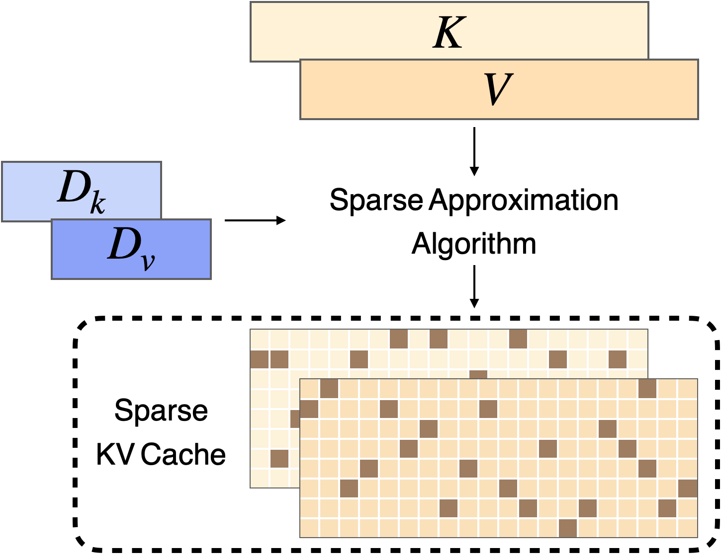
(a) Prefilling Stage

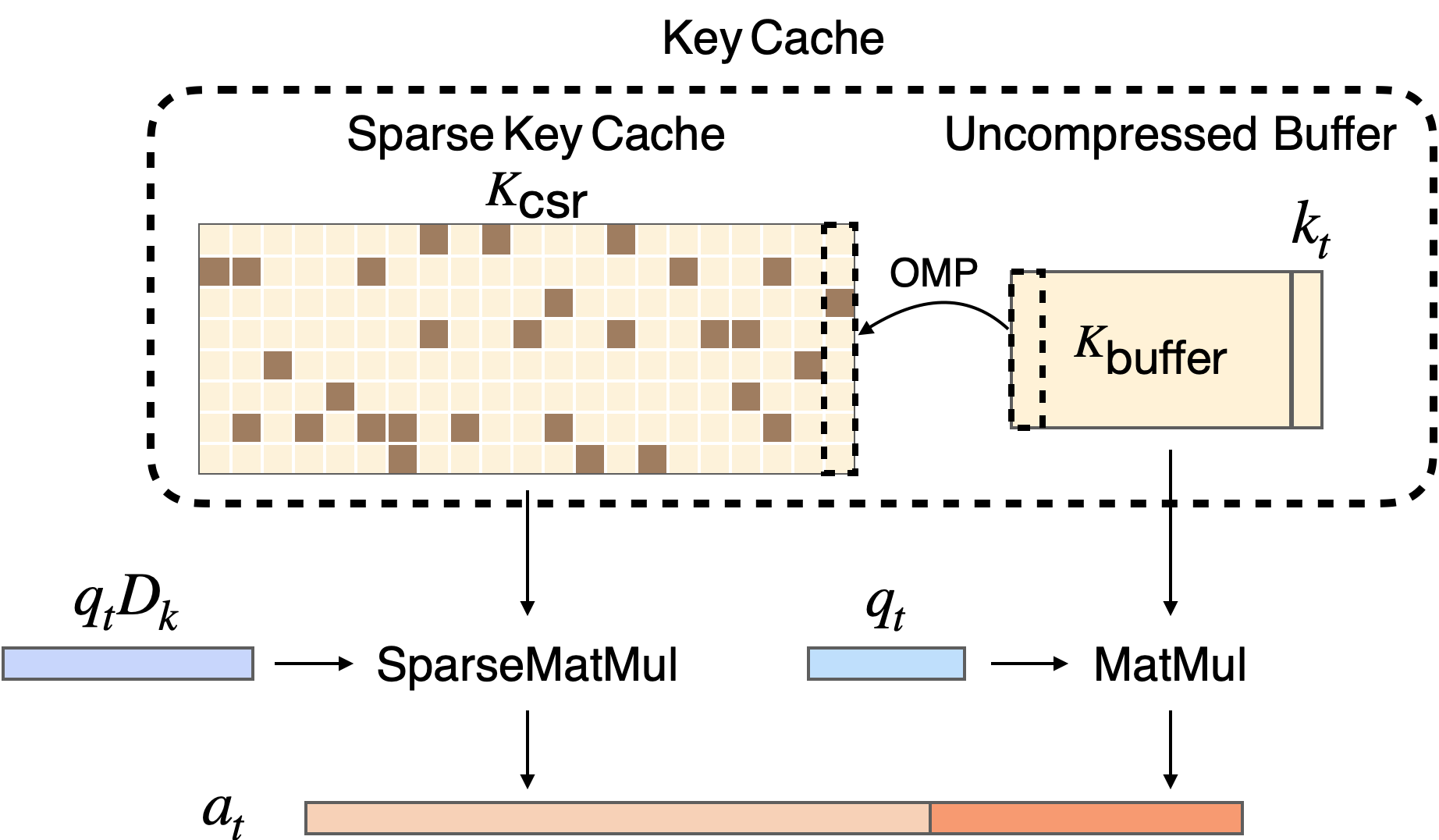
(b) Decoding Stage

Figure 2: (a) Prefilling: Following attention computation, Lexico uses OMP to find sparse representations of the KV vectors ($3\text{-}8\times$ smaller). (b) Decoding: Key cache consists of the compressed sparse key cache, ${\bm{K}}_{\text{csr}}$, and an full-precision buffer, ${\bm{K}}_{\text{buffer}}$, for the most recent tokens. ${\bm{q}}_{t}$, ${\bm{k}}_{t}$ represent the query, key vectors for the newly generated token. Computation is reduced by computing the query-dictionary product, ${\bm{q}}_{t}{\bm{D}}_{k}$, then multiplying ${\bm{K}}_{\text{csr}}$, to get the pre-softmax attention score.

Towards this end, we propose Lexico, a universal dictionary that serves as an overcomplete basis, which can sparsely decompose and reconstruct the KV cache with sufficiently small reconstruction error that can be directly controlled via the level of sparsity of each reconstruction.

In Section 3.2, we report our observation that a subset of key vectors cluster near each other, even though the keys are from different inputs, while some cluster on different subspaces. To take advantage of such a low-dimensional structure, we draw inspiration from compressed sensing and dictionary learning, areas of statistical learning and signal processing that developed algorithms for information compression across various applicaiton domains (Candès et al., 2006; Donoho, 2006; Dong et al., 2014; Metzler et al., 2016).

Lexico is simple to learn, can be applied off-the-shelf for KV cache compression, and only occupies small constant memory regardless of input or batch size. Methodologically, Lexico utilizes both sparsity-based compression (steps 1 and 2) and quantization (step 3) in three straightforward steps:

1. Dictionary pretraining: For our experiments, we train a dictionary on WikiText-103 (Merity, 2016) for each model. This dictionary is only trained once and used universally across all tasks. It only occupies constant memory and does not increase with batch size. We note that this dictionary can be trained from richer sources to improve the overall performance of our sparse approximation algorithms.

2. Sparse decomposition: During prefilling and decoding (Figure 2), Lexico decomposes key-value pairs into a sparse linear combination, which consists of $s$ pairs of reconstruction coefficients and dictionary indices pointing. This step by itself provides high compression rates.

3. Lightweight sparse coefficients: We obtain higher KV cache compression rates by representing the sparse coefficients in 8 bits instead of FP16. Lowering precision to 8 bits yields minimal degradation. Lexico theoretically allows us to compress more than 2-bit quantization ($1/8$ of FP16 KV cache size) if $s\leq 10$ when head dimension is $128$.

Overall, we make the following contributions:

• Near-lossless performance: Given similar memory requirements, Lexico performs on par with or better than baseline quantization methods on challenging language tasks, such as LongBench (Bai et al., 2023) and GSM8K (Cobbe et al., 2021).

• Compression rates beyond 2-bits: Lexico’s sparsity parameter enables both wider and more fine-grained control over desired memory usage. This allows us to explore performance when using under 15-20% of the original KV cache size, a low-memory regime previous compression methods could not explore.

• Universality: Instead of an input-dependent dictionary, we find a sufficiently small universal dictionary (per model) that can be used for all tasks and across multiple users. Advantageously, such dictionary does not scale with batch size and can be used off-the-shelf.

2 Related Work

Prior work on KV cache optimization has explored both training-stage and deployment-focused strategies to improve the efficiency of LLMs. On the deployment side, Kwon et al. (2023) introduce a Paged Attention mechanism and the popular vLLM framework, which adapt CPU-style page memory to map KV caches onto GPU memory using a mapping table, thereby minimizing memory fragmentation and leveraging custom CUDA kernels for efficient inference. While there is a significant and important line of research in this direction (Lin et al., 2024; Qin et al., 2024), this direction is orthogonal to our work and can often be used in tandem with quantization.

Current post-training KV cache compression methods can broadly be categorized into eviction, quantization, and merging. Zhang et al. (2024) introduced H2O, which uses attention scores to selectively retain tokens while preserving recent ones that are strongly correlated with current tokens. Multiple works discuss various heuristics and algorithms to find which tokens can be discarded, while some works find how to complement evictions methods (Ge et al., 2023; Li et al., 2024; Liu et al., 2024a; Devoto et al., 2024; Dong et al., 2024). For this line of work, there is a chance that evictions can work well together with Lexico, as Liu et al. (2024a) have successfully combined quantization and eviction.

Quantization methods have also played a crucial role in reducing KV cache size without compromising model performance. Although there is a flurry of work, we only mention those that are most relevant to our discussion and methodology. Hooper et al. (2024) identified outlier channels in key matrices and developed KVQuant, while Liu et al. (2024b) pursue a similar per-channel strategy in KIVI. Further extending these ideas, Yue et al. (2024) presented WKVQuant, which quantizes model weights as well as KV cache using two-dimensional quantization. Kang et al. (2024) follow similar per-channel key and per-token value quantization as KIVI, but with additional low-rank and sparse structures to manage quantization errors.

3 KV Cache Compression with Dictionaries

3.1 Background & Notation

During autoregressive decoding in Transformer, the key and value states for preceding tokens are independent of subsequent tokens. As a result, these key and value states are cached to avoid recomputation, thereby accelerating the decoding process.

Let the input token embeddings be denoted as ${\bm{X}}\in{\mathbb{R}}^{l_{\text{seq}}\times d}$, where $l_{\text{seq}}$ and $d$ are the sequence length and model hidden dimension, respectively. For simplicity, we focus on a single layer and express the computation of query, key, and value states at each attention head during the prefilling stage as:

$${\bm{Q}}^{(h)}={\bm{X}}{\bm{W}}_{q}^{(h)},\quad{\bm{K}}^{(h)}={\bm{X}}{\bm{W}}_{k}^{(h)},\quad{\bm{V}}^{(h)}={\bm{X}}{\bm{W}}_{v}^{(h)},$$ (1)

where ${\bm{W}}_{q}^{(h)},{\bm{W}}_{k}^{(h)},{\bm{W}}_{v}^{(h)}\in\mathbb{R}^{d\times m}$ are the model weights with $m$ representing the head dimension.

Let $t$ represent the current step in the autoregressive decoding, and let ${\bm{x}}_{t}\in\mathbb{R}^{1\times d}$ denote the embedding of the newly generated token. The KV cache up to but not including the current token, are denoted as ${\bm{K}}_{t-1}^{(h)}$ and ${\bm{V}}_{t-1}^{(h)}$, respectively. The typical output computation for each attention head ${\bm{h}}_{t}^{(h)}$ using the KV cache can be expressed as:

$${\bm{h}}_{t}^{(h)}=\mathrm{Softmax}\left({\bm{q}}_{t}^{(h)}\left({\bm{K}}_{t-1}^{(h)}\parallel{\bm{k}}_{t}^{(h)}\right)^{\top}/{\sqrt{m}}\right)\left({\bm{V}}_{t-1}^{(h)}\parallel{\bm{v}}_{t}^{(h)}\right),$$ (2)

where ${\bm{q}}_{t}^{(h)},{\bm{k}}_{t}^{(h)},{\bm{v}}_{t}^{(h)}$ represent the query, key, and value vectors for the new token embedding ${\bm{x}}_{t}$. Here, $\parallel$ denotes concatenation along the sequence length dimension.

3.2 Sparse Approximation

Given a dictionary, our goal is to decompose and represent KV cache efficiently, i.e., approximate a vector ${\bm{k}}\in\mathbb{R}^{m}$ as a linear combination of a few vectors (atoms) from an overcomplete dictionary ${\bm{D}}\in\mathbb{R}^{m\times N}$. This reconstruction is given by ${\bm{k}}={\bm{D}}{\bm{y}}$, where ${\bm{y}}\in\mathbb{R}^{N}$ is the sparse representation vector such that $s=||{\bm{y}}||_{0}$. For implementation, ${\bm{y}}$ only requires space proportional to $s$, not $N$.

We hypothesize that the KV cache, like other domains where sparse approximation is effective, contains inherent redundancy that can be leveraged for efficient compression. For instance, Figure 3 presents pairwise cosine similarity plots for keys generated during inference on a random subset of the WikiText dataset. Here, we observe that key vectors cluster in multiple different subspaces. Dictionary learning can take advantage of such redundancy, enabling KV vectors to be represented by a compact set of atoms with only a few active coefficients.

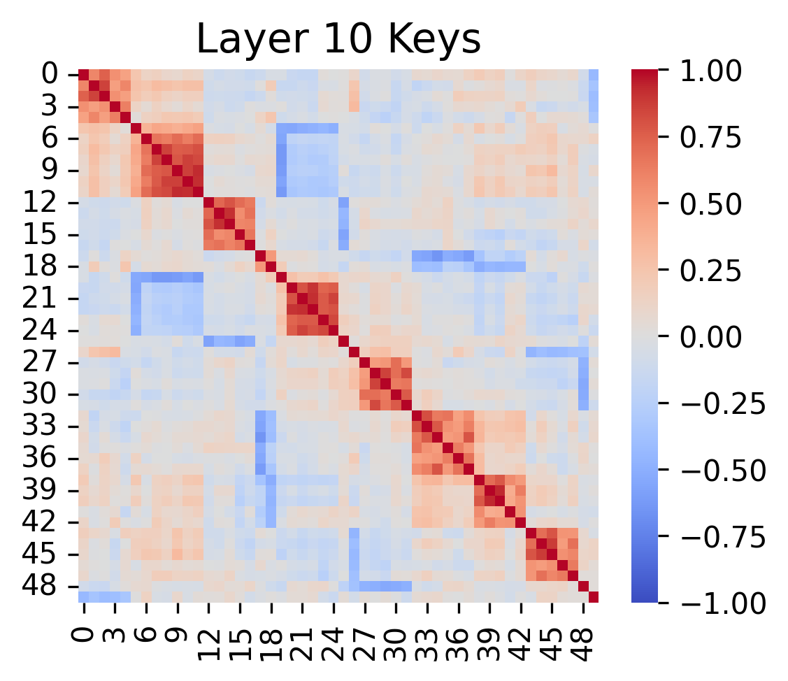
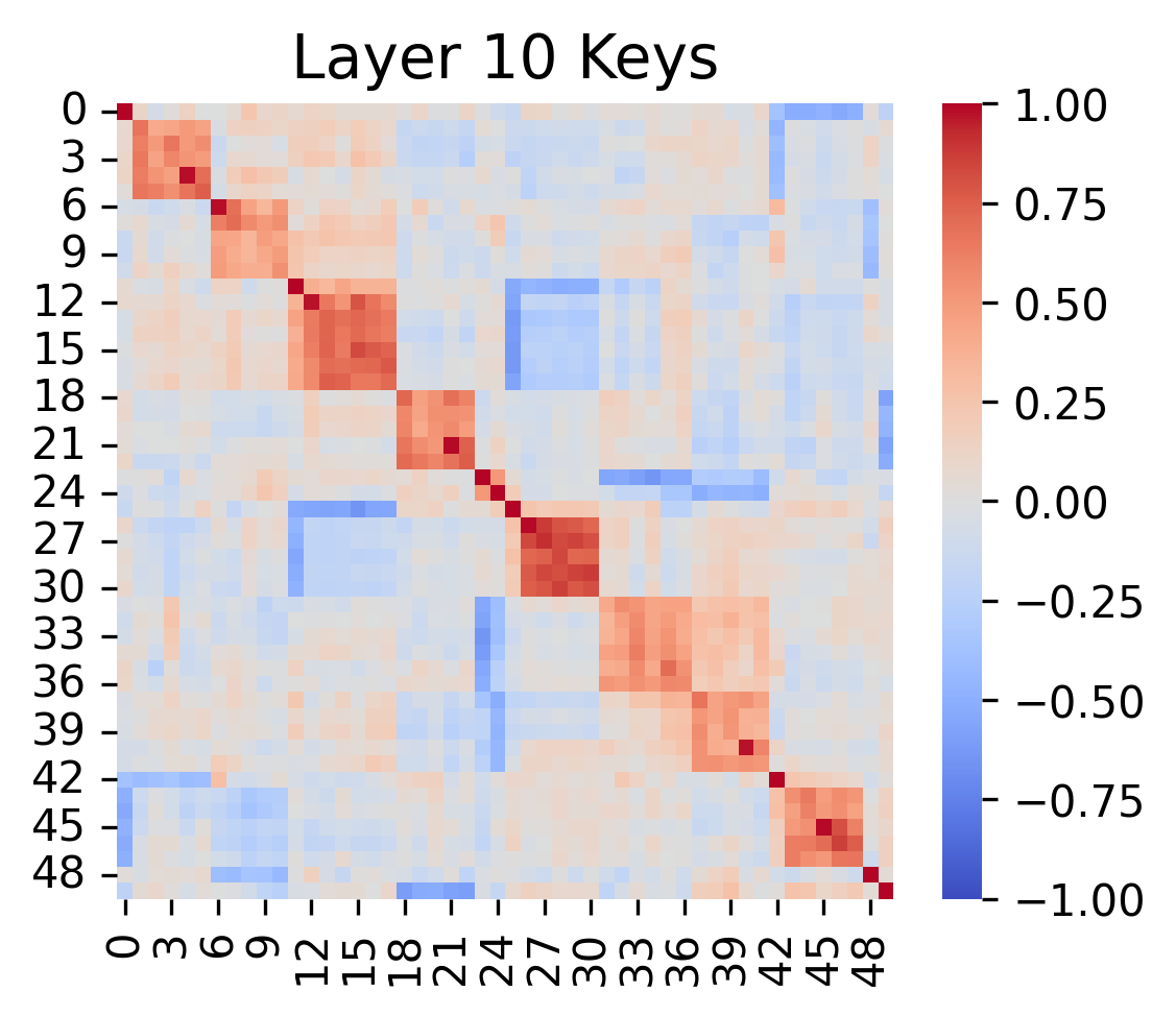
Figure 3: Left shows a pairwise cosine similarity matrix between key vectors generated from one input text from all heads in Layer 10 of Llama-3.1-8B-Instruct. Keys are sorted by similarity to demonstrate the clusters. Right shows the similarity matrix between key vectors from two different input texts. These plots indicate that there may exist a mixture of low-dimensional subspaces in the space of all possible keys, a hypothesis that naturally leads to dictionary learning.

Sparse approximation, which aims to find ${\bm{y}}$ with minimum sparsity given ${\bm{k}}$ and ${\bm{D}}$, while ensuring a small reconstruction error, is NP-hard. This optimization problem is typically formulated as:

$$\underset{{\bm{y}}}{\text{min}}\left\|{\bm{y}}\right\|_{0}\text{subject to}\left\|{\bm{k}}-{\bm{D}}{\bm{y}}\right\|_{2}\leq\delta\left\|{\bm{k}}\right\|_{2}\text{ for some relative error threshold }\delta>0$$ (3)

In this work, we adopt Orthogonal Matching Pursuit (OMP) as the sparse approximation algorithm. Given an input key or value vector ${\bm{k}}$, a dictionary ${\bm{D}}$, and a target sparsity $s$, OMP iteratively selects dictionary atoms to minimize the $\ell_{2}$-reconstruction error, with the process continuing until the specified sparsity $s$ is reached. Our implementation of OMP builds on advanced methods that utilize properties of the Cholesky inverse (Zhu et al., 2020) to optimize performance. Additionally, we incorporate implementation details from Lubonja et al. (2024) for efficient batched GPU execution and extend it to include an extra batch dimension, allowing for parallel processing across multiple dictionaries. The full algorithm is detailed in Appendix A.

3.3 Learning Layer-specific Dictionaries

Layer-specific dictionaries.

While the sparse approximation algorithm is crucial, achieving a high compression ratio relies heavily on well-constructed dictionaries. In this section, we describe the process for training the dictionaries used in Lexico. We adopt distinct dictionaries for the key and value vectors in each transformer layer due to their different functionalities. We denote the key and value dictionaries at each layer as ${\bm{D}}_{k}$ and ${\bm{D}}_{v}\in\mathbb{R}^{m\times N}$, where $N$ is the fixed dictionary size. With $N=1024$, the dictionaries add an additional 16.8MB to the model’s storage requirements for 7B/8B models.

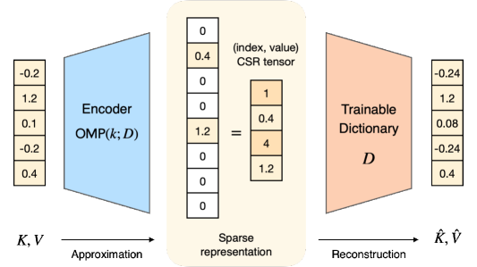
Figure 4: Dictionary Learning of Lexico. We train a linear layer ${\bm{D}}$ (our dictionary) that minimizes $\ell_{2}$-reconstruction error of KV cache. The KV cache of layer $i$ are used as training data for dictionary ${\bm{D}}^{(i)}$. Each step, we apply OMP with fixed ${\bm{D}}$ to represent KV as a vector of sparse coefficients; we then perform a step of gradient descent on ${\bm{D}}$ and repeat the process. A sparse vector can be efficiently stored as a CSR, using a tuple of 16-bit index and 8-bit value.

As shown in Figure 4, we train layer-specific KV dictionaries through direct gradient-based optimization. For a given key or value vector, denoted as ${\bm{k}}\in\mathbb{R}^{m}$ and a dictionary ${\bm{D}}\in\mathbb{R}^{m\times N}$, the OMP algorithm approximates the sparse representation ${\bm{y}}\in\mathbb{R}^{N}$. This process is parallelized across multiple dictionaries, but for simplicity, we present the notation for a single dictionary. The dictionary training objective minimizes the $\ell_{2}$ norm of the reconstruction error, with the loss function $\mathcal{L}=\left\|{\bm{k}}-{\bm{D}}{\bm{y}}\right\|_{2}^{2}$. We enforce unit norm constraints on the dictionary atoms by removing any gradient components parallel to the atoms before applying updates.

Training.

The dictionaries are trained on KV pairs generated from the WikiText-103 dataset using Adam (Kingma & Ba, 2014) with a learning rate of 0.0001 and a cosine decay schedule over 20 epochs. The dictionaries are initialized with a uniform distribution, following the default initialization method for linear layers in PyTorch. For Llama-3.1-8B-Instruct, with a sparsity of $s=32$ and a dictionary size of $N=1024$, the training process takes about 2 hours on an NVIDIA A100 GPU.

Table 1: Reconstruction error. Relative reconstruction errors of different methods when training dictionary of size $1024$ and sparsity $s=32$ on WikiText-103. Sparse Autoencoder is a two-layer perceptron with hard top-$k$ thresholding as activation (encoder as a linear layer + activation in Figure 4). Lexico is optimized using OMP as encoder. KV cache is generated from Llama-3.1-8B-Instruct.

Test Dataset	Lexico	Sparse Autoencoder	Random Dictionaries
WikiText-103	$\mathbf{0.17}\pm 0.06$	$0.20\pm 0.05$	$0.27\pm 0.02$
CNN/DailyMail	$\mathbf{0.19}\pm 0.05$	$0.22\pm 0.04$	$0.27\pm 0.02$
IMDB	$\mathbf{0.18}\pm 0.05$	$0.22\pm 0.05$	$0.27\pm 0.02$
TweetEval	$\mathbf{0.18}\pm 0.06$	$0.21\pm 0.05$	$0.27\pm 0.02$

We demonstrate our trained dictionaries reconstruct and generalize better than dictionaries trained using sparse autoencoders (similarly to those from Makhzani & Frey (2013); Bricken et al. (2023)) across several corpora in Table 1. Our method consistently achieves lower relative reconstruction errors, such as $0.19\pm 0.05$ on out-of-domain dataset CNN/DailyMail, and this trend is consistent across other datasets.

Despite being trained only on WikiText-103, Lexico dictionaries demonstrate a degree of universality: our dictionaries achieve lower test loss on out-of-domain datasets such as TweetEval than the test loss on WikiText-103 for sparse autoencoders, offering significant compression with minimal reconstruction error. In the next subsection, we explore how low $\ell_{2}$-reconstruction loss translates to strong performance preservation in language modeling.

3.4 Prefilling and Decoding with Lexico

During the prefilling stage, each layer generates the KV vectors for the input tokens, as illustrated in Figure 2(a). Lexico uses full-precision KV vectors for attention computation, which are then passed to subsequent layers. Subsequently, OMP finds the sparse representations of the KV vectors using layer-specific key and value dictionaries, ${\bm{D}}_{k}$ and ${\bm{D}}_{v}$.

The compressed key and value caches are denoted as ${\bm{K}}_{\text{csr}},{\bm{V}}_{\text{csr}}\in\mathbb{R}^{l_{\text{seq}}\times N}$ and replace the full-precision KV cache. The reconstruction of the KV cache is performed as follows:

$$\hat{{\bm{K}}}={\bm{K}}_{\text{csr}}{\bm{D}}_{k}^{\top},\quad\hat{{\bm{V}}}={\bm{V}}_{\text{csr}}{\bm{D}}_{v}^{\top}$$ (4)

Recall that at the $t$-th iteration of autoregressive decoding, each layer receives ${\bm{q}}_{t}$, ${\bm{k}}_{t}$, and ${\bm{v}}_{t}$, the query, key, and value vectors corresponding to the newly generated token. Similarly to prior work (Liu et al., 2024b; Kang et al., 2024), we find that keeping a small number of recent tokens in full precision improves the generative performance of the model. To achieve this, we introduce a buffer that temporarily stores recent tokens in an uncompressed state. The KV vectors stored in the buffer are denoted as ${\bm{K}}_{\text{buffer}},{\bm{V}}_{\text{buffer}}\in\mathbb{R}^{n_{b}\times m}$, where $n_{b}$ is the number of KV vectors in the buffer. The key cache up to, but not including the new token at iteration $t$, is then reconstructed as follows:

$$\hat{{\bm{K}}}_{t-1}={\bm{K}}_{\text{csr}}{\bm{D}}_{k}^{\top}\parallel{\bm{K}}_{\text{buffer}}$$ (5)

Substituting this reconstruction into the Equation 2, the attention weights for each head ${\bm{a}}_{t}^{(h)}$ are computed as:

$${\bm{a}}_{t}^{(h)}=\text{Softmax}\left({\bm{q}}_{t}^{(h)}({\bm{K}}_{\text{csr}}^{(h)}{\bm{D}}_{k}^{\top}\parallel{\bm{K}}_{\text{buffer}}^{(h)}\parallel{\bm{k}}_{t}^{(h)})^{\top}/\sqrt{m}\right)$$ (6)

A key implementation is that attention for the compressed sparse key cache and the uncompressed key cache is computed separately. For compressed sparse key cache, we first compute the product ${\bm{q}}_{t}^{(h)}{\bm{D}}_{k}$ before we multiply ${\bm{K}}_{\text{csr}}$, directly calculating the pre-softmax attention scores for compressed tokens. Attention for the buffer tokens is computed as usual. These scores are then concatenated with softmax to produce the final attention weights (Figure 2(b)). This process is formalized as:

$${\bm{a}}_{t}^{(h)}=\text{Softmax}\left(\left({\bm{q}}_{t}^{(h)}{\bm{D}}_{k}{\bm{K}}_{\text{csr}}^{(h)\top}\mid{\bm{q}}_{t}^{(h)}({\bm{K}}_{\text{buffer}}^{(h)}\parallel{\bm{k}}_{t}^{(h)})^{\top}\right)/{\sqrt{m}}\right),$$ (7)

where $\mid$ represents concatenation along columns for attention scores.

When the buffer reaches capacity, OMP compresses the KV vectors for the oldest $n_{a}$ tokens in the buffer. This process is independent of the attention computation for the newest token and can therefore be performed in parallel.

Time and space complexity.

The sparse representations are stored in CSR format, with values encoded in FP8(E4M3), and all indices, including offsets, are stored as int16. Each row in CSR corresponds to a single key or value vector. For a given sparsity level $s$, the memory usage includes: nonzero values ($s$ bytes), dictionary indices ($2s$ bytes), and the offset array (2 bytes), resulting in a total size of $3s+2$ bytes. For a head dimension of 128, a fully uncompressed vector using FP16 takes $256$ bytes, yielding a memory usage of $\frac{3s+2}{256}\times 100\approx 1.17s\%$ (e.g., $37.5\%$ for $s=32$).

In terms of time complexity, computing ${\bm{q}}_{t}{\bm{K}}_{t}^{\top}$ for a single head requires $O(l_{\text{seq}}m)$ multiplications. On the other hand, ${\bm{q}}_{t}{\bm{D}}_{k}{\bm{K}}_{\text{csr}}^{\top}$ needs $O(Nm+l_{\text{seq}}s)$ multiplications. This means that our computation is particularly well-suited for long-context tasks when $l_{\text{seq}}>m$ where $m$ is anywhere between 1024 and 4096. For short contexts when $l_{\text{seq}}<m$, our method only adds a small overhead to attention computation in actuality.

4 Experiments

Setup.

We evaluate our method on various models (Llama-3-8B, Llama-3.1-8B-Instruct, Llama-3.2-1B-Instruct, Llama-3.2-3B-Instruct, Mistral-7B-Instruct), using dictionaries trained on WikiText-103, as done in Section 3.3. To assess the effectiveness of Lexico in memory reduction while maintaining long-context understanding, we conduct experiments on selected tasks from LongBench (Bai et al., 2023), following the setup of Liu et al. (2024b). See Table 8 in Appendix B for task details.

Additionally, we evaluate generative performance on complex reasoning tasks, such as GSM8K (Cobbe et al., 2021) with 5-shot prompting and MMLU-Pro Engineering/Law (Wang et al., 2024a) with zero-shot chain-of-thought. We choose these MMLU-Pro subjects since they are deemed the most difficult as they require complex formula derivations or deep understanding of legal knowledge intricacies. We compare our method against two kinds of KV cache compression methods: namely, quantization-based compression and eviction-based compression. For quantization-based methods, we evaluate KIVI (Liu et al., 2024b), ZipCache (He et al., 2024), and the Hugging Face implementation for per-token quantization. For eviction-based methods, we evaluate PyramidKV (Cai et al., 2024) and SnapKV (Li et al., 2024).

We refer to the 4-bit and 2-bit versions of KIVI as KIVI-4 and KIVI-2, respectively, and denote its quantization group size as $g$.

We report KV size as the average percentage of the compressed cache relative to the full cache at the end of generation. Lexico’s sparsity $s$ is set to match the KV size of the baseline.

Hyperparameter settings.

For both experiments, Lexico uses a dictionary size of $N=4096$, a buffer size of $n_{b}=128$, and an approximation window size $n_{a}=1$, compressing the oldest token with each new token generated. For KIVI-4 and KIVI-2, we use a quantization group size of $g=32$ and a buffer size of $n_{b}=128$ , as is tested and recommended in Liu et al. (2024b), for LongBench. For GSM8K and MMLU-Pro, we test for stronger memory savings, so we use $g=64$ and $n_{b}=64$ for KIVI.

4.1 Experimental Results

LongBench results.

Table 2 presents the performance of Lexico and KIVI on LongBench tasks. Lexico demonstrates better performance than KIVI with similar or even smaller KV sizes. Notably, Lexico enables exploration of extremely low memory regimes that KIVI-2 cannot achieve. At a memory usage of just $12.4\%$ KV size, Lexico maintains reasonable long-context understanding, with only 5.6$\%p$ and 4.4$\%p$ performance loss on Llama-3.1-8B-Instruct and on Mistral-7B-Instruct-v0.3, respectively, compared to the full cache (FP16). The largest performance loss comes from tasks with the lowest full cache accuracy, Qasper, yet there is almost no loss in simpler tasks, such as TriviaQA. This indicates that difficult tasks that require more complex understanding are much more sensitive to performance loss. Hence, it is important to evaluate on GSM8K, one of the harder natural language reasoning tasks, as we do next.

Table 2: Experimental results on LongBench. For Lexico, we use $N=4096$ as the dictionary size and $n_{b}=128$ as the buffer size. For KIVI, we use $g=32$ (group size for quantization) and $n_{b}=128$ (buffer size). Sparsity level $s$ is set to match average KV size of KIVI, while $s=8$ corresponds to cache size unattainable by common 2-bit quantizations. Full cache is in FP16.

Method	KV Size	Qasper	QMSum	MultiNews	TREC	TriviaQA	SAMSum	LCC	RepoBench-P	Average
Llama-3.1-8B-Instruct
Full Cache	$100\%$	$22.54$	$24.57$	$27.44$	$72.5$	$91.65$	$43.47$	$63.15$	$56.76$	$50.26$
KIVI-4	$33.2\%$	$\mathbf{22.83}$	$23.72$	$\mathbf{27.95}$	$71.0$	$90.39$	$\mathbf{44.25}$	$\mathbf{62.93}$	$55.48$	$49.78$
Lexico s=24	$30.6\%$	$21.68$	$\mathbf{24.25}$	$27.20$	$\mathbf{72.5}$	$\mathbf{91.58}$	$42.93$	$62.92$	$\mathbf{56.51}$	$\mathbf{49.95}$
KIVI-2	$21.1\%$	$13.77$	$22.72$	$\mathbf{27.35}$	$71.0$	$90.85$	$\mathbf{43.53}$	$62.03$	$53.00$	$48.03$
Lexico s=16	$21.4\%$	$\mathbf{15.45}$	$\mathbf{23.13}$	$25.78$	$\mathbf{72.5}$	$\mathbf{92.25}$	$42.02$	$\mathbf{63.01}$	$\mathbf{55.58}$	$\mathbf{48.71}$
Lexico s=8	$\mathbf{12.4\%}$	$11.66$	$21.04$	$22.35$	$60.0$	$91.01$	$40.30$	$59.60$	$51.46$	$44.68$
Mistral-7B-Instruct-v0.3
Full Cache	$100\%$	$41.58$	$25.69$	$27.76$	$76.0$	$88.59$	$47.58$	$59.37$	$60.60$	$53.40$
KIVI-4	$33.2\%$	$40.37$	$24.51$	$\mathbf{27.75}$	$74.0$	$88.36$	$\mathbf{47.56}$	$58.49$	$58.31$	$52.42$
Lexico s=24	$30.6\%$	$\mathbf{41.01}$	$\mathbf{25.32}$	$27.51$	$\mathbf{76.0}$	$\mathbf{88.84}$	$46.27$	$\mathbf{59.98}$	$\mathbf{59.44}$	$\mathbf{53.05}$
KIVI-2	$21.1\%$	$38.24$	$24.08$	$\mathbf{26.99}$	$74.5$	$88.34$	$\mathbf{47.66}$	$57.51$	$56.46$	$51.72$
Lexico s=16	$21.4\%$	$\mathbf{40.34}$	$\mathbf{24.97}$	$26.36$	$\mathbf{76.0}$	$\mathbf{89.31}$	$45.84$	$\mathbf{59.31}$	$\mathbf{59.50}$	$\mathbf{52.70}$
Lexico s=8	$\mathbf{12.4\%}$	$33.03$	$22.80$	$22.85$	$68.5$	$87.85$	$43.10$	$56.66$	$56.85$	$48.96$

GSM8K results.

The performance of Lexico on GSM8K compared to KIVI is shown in Table 3. With a KV size of $36.9\%$, Lexico on Llama 8B models experiences a slight accuracy drop of less than $3\%p$, underperforming KIVI-4 at a similar KV size. However, in the lower memory regime near $25\%$ KV size, Lexico significantly outperforms KIVI-2, achieving a higher accuracy by $8.2\%p$ on the Llama-3-8B model and $7.1\%p$ on the Llama-3.1-8B-Instruct model. These results highlight the robustness of Lexico in low-memory settings, demonstrating that low reconstruction error can be achieved using only a few atoms from our universal dictionary. To further test the resilience of Lexico, we set the sparsity to $s=4$, observing a noticeable drop in accuracy on the Llama-3.1-8B-Instruct model. Despite this, both Llama models maintain an accuracy above $40\%$, which is remarkable given that only 4 atoms from Lexico were used for each key-value vector, utilizing just $15.8\%$ of the full cache, including the buffer.

The performance of Lexico on the Mistral-7B-Instruct model is even more impressive. We demonstrate that for Mistral, Lexico not only outperforms KIVI-4 and KIVI-2 but also achieves higher accuracy with even less memory usage. We also evaluate Lexico with $s=4$ on the Mistral model and observe an accuracy of $39.2\%$, further demonstrating robustness in low-memory settings.

Table 3: Experimental results on GSM8K. For Lexico, we use $N=4096$ as the dictionary size and $n_{b}=128$ as the buffer size. For KIVI, we use $g=64$ (group size for quantization) and $n_{b}=64$ (buffer size). Sparsity level $s$ is set to match the average KV size of KIVI, while $s=4$ corresponds to cache size unattainable by common 2-bit quantizations. Full cache is in FP16. We include example generations of KIVI and Lexico in Appendix D.1.

(a) Llama 3.x 8B Models

Method	KV Size	Llama-3-8B	3.1-8B-Instruct
Full Cache	$100\%$	$49.89$	$79.61$
KIVI-4	$38.2\%$	$\mathbf{49.13}$	$\mathbf{78.17}$
Lexico s=24	$36.9\%$	$48.29$	$76.88$
KIVI-2	$25.7\%$	$40.56$	$67.93$
Lexico s=14	$26.1\%$	$\mathbf{48.75}$	$\mathbf{75.06}$
Lexico s=4	$\mathbf{15.8\%}$	$40.03$	$51.71$

(b) Mistral 7B v0.3 Model

Method	KV Size	7B-Instruct
Full Cache	$100\%$	$48.60$
KIVI-4	$38.2\%$	$48.52$
Lexico s=20	$32.7\%$	$\mathbf{48.60}$
KIVI-2	$25.7\%$	$42.91$
Lexico s=10	$22.0\%$	$\mathbf{44.35}$
Lexico s=4	$\mathbf{15.8\%}$	$39.20$

Results across model sizes and baselines.

We illustrate the trade-off between memory usage and performance across six different KV cache compression methods on Llama models (1B, 3B, and 8B) in Figure 1. For all three model sizes, Lexico consistently lies on the Pareto frontier, achieving higher scores than other compression methods at similar KV cache budget sizes. Notably, Lexico demonstrates greater robustness at smaller model scales, with larger performance gaps observed for the 1B and 3B models. In the extremely low-memory regime below $20\%$, where quantization methods such as KIVI and ZipCache cannot achieve feasible cache sizes, Lexico achieves superior performance. Furthermore, while eviction-based methods (SnapKV, PyramidKV) can operate in these extremely low-memory settings, their performance lags significantly behind due to their incompatibility with GQA, making Lexico the effective choice for stringent memory constraints. We also evaluate Lexico on a larger model, Qwen2.5-14B-Instruct, with its weights quantized to 4 bits, comparing it against quantization methods. The results, illustrated in Figure 6, show that Lexico achieves a higher GSM8K score than KIVI under similar KV cache budgets. Additionally, Lexico enables higher compression ratios than 2-bit quantization methods, facilitating deployment under extreme memory-constrained scenarios.

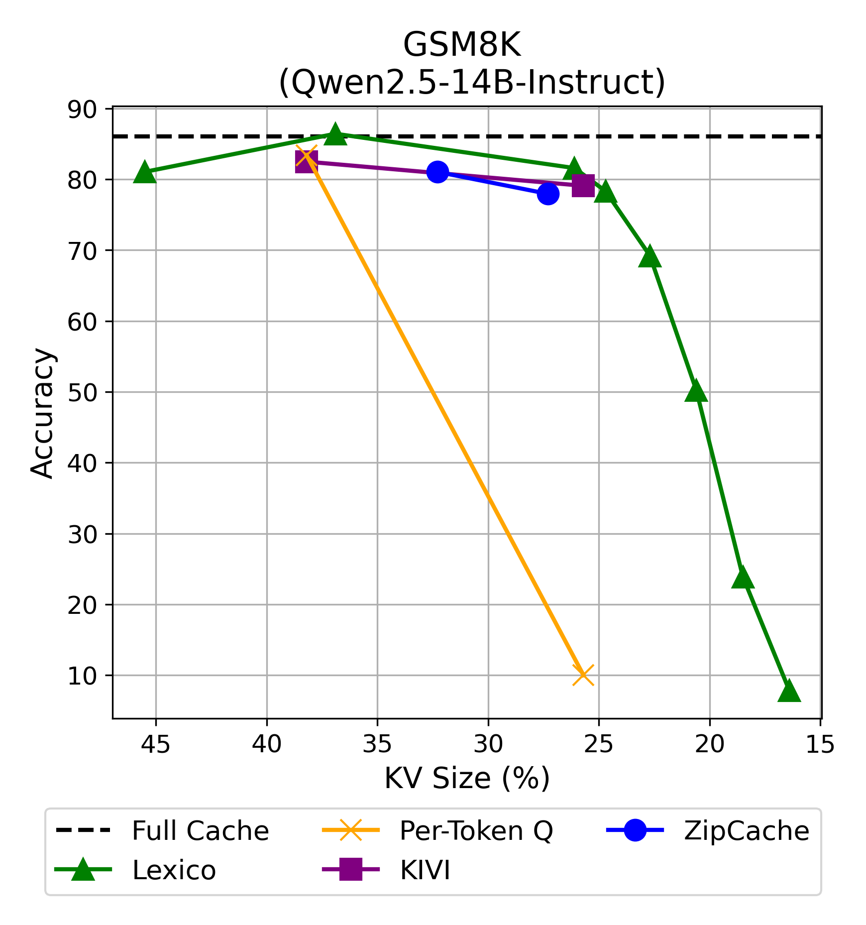
Figure 5: Memory usage vs. performance of Qwen2.5-14B-Instruct with Lexico on GSM8K. We compare the performance of Lexico against quantization methods on Qwen2.5-14B-Instruct, with its weights quantized to 4 bits. For Lexico, we use $N=4096$ as the dictionary size and $n_{b}=128$ as the buffer size.

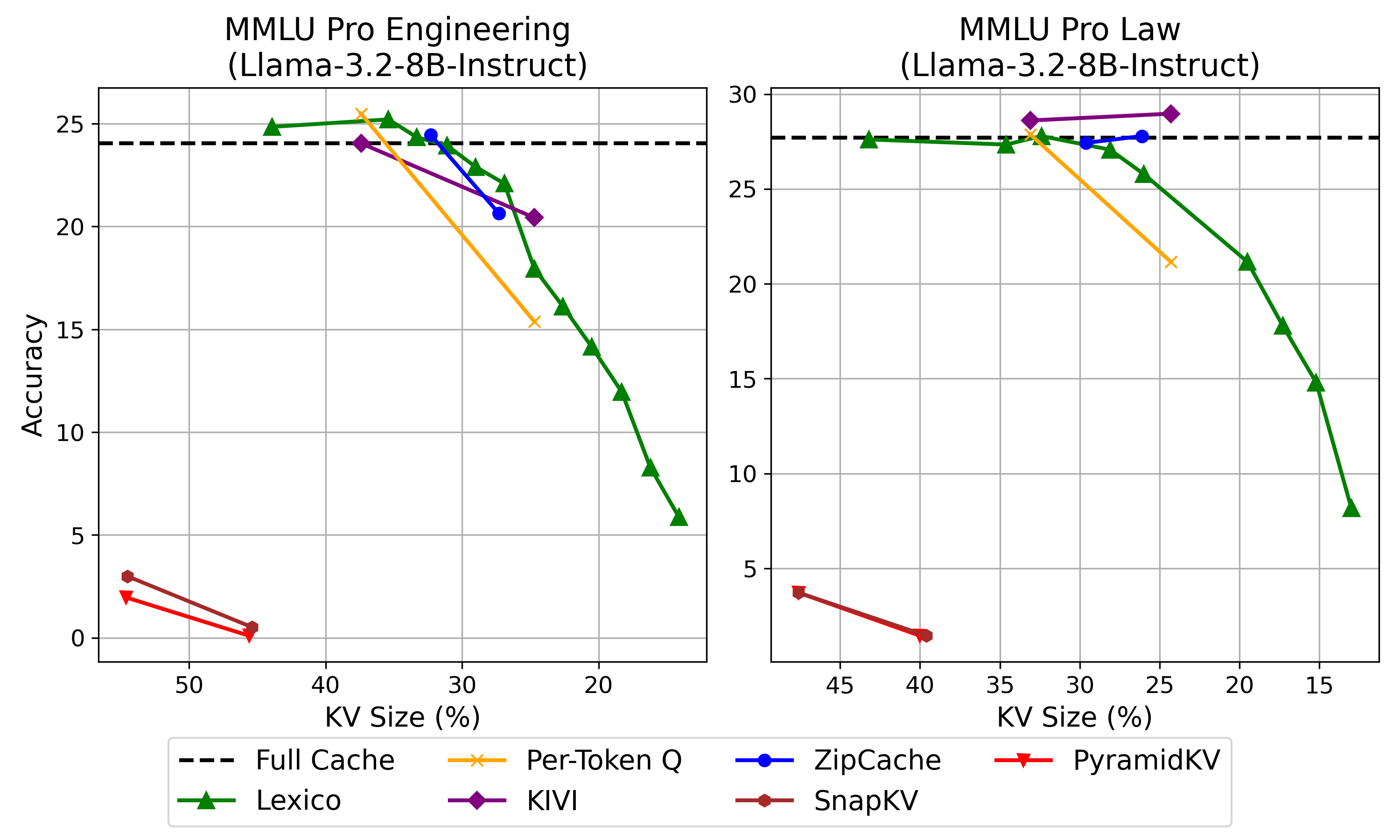
Figure 6: Memory usage vs. performance of Llama-3.2-8B-Instruct with Lexico on MMLU-Pro Engineering/Law. For Lexico, we use $N=4096$ as the dictionary size and $n_{b}=128$ as the buffer size. Lexico often outperforms both eviction-based methods (SnapKV, PyramidKV) and quantization-based methods (per-token quantization, KIVI, ZipCache). For Law, our method slightly underperforms around 25%, but in lower memory regimes, our method still outperforms any other baseline.

MMLU-Pro results.

Figure 6 illustrates the trade-offs between memory usage and performance for Lexico on the MMLU-Pro Engineering and Law subjects using the Llama-3.1-8B-Instruct model. Lexico outperforms eviction-based methods like SnapKV and PyramidKV across all memory settings, though its performance is comparable to quantization-based methods such as KIVI and ZipCache. However, in a low memory regime below 20% cache, our method still outperforms any other baseline. This highlights that Lexico supports a wide range of compression ratios quite effectively and that our dictionary is generalizable across input distributions.

4.2 Ablation Study

In this subsection, we ablate the various components of Lexico and how it may influence memory complexity and task performance.

4.2.1 Error Thresholding in Sparse Approximation

Lexico also supports a quality-controlled method for memory saving by allowing early termination of the sparse approximation process when a predefined error threshold is met. This approach conserves memory that would otherwise be used for marginal improvements in approximation quality.

For the error thresholding ablation study, detailed results are provided in Table 4. We set a maximum sparsity of 32, corresponding to the maximum number of iterations for the OMP algorithm. However, if the reconstruction error at any iteration falls below a predefined error threshold, we let the OMP terminate early, saving memory that would otherwise be used for minor approximation improvements. This approach is particularly compatible with OMP, as its greedy nature ensures that early termination yields the same results as using higher sparsity (less non-zero elements). Additionally, OMP inherently computes the residual at each iteration, allowing for continuous evaluation of the relative reconstruction error without requiring any additional computation.

Table 4: Impact of error thresholding on LongBench performance and memory usage. The table presents the performance of Lexico on the Llama-3.1-8B-Instruct model at various reconstruction error thresholds ($\delta$) for early termination of the sparse approximation algorithm. A dictionary size of $N=1024$ and FP16 precision for the values of the CSR tensors are used.

Threshold ($\delta$)	KV Size	Qasper	QMSum	MultiNews	TREC	TriviaQA	SAMSum	LCC	RepoBench-P	Average
Llama-3.1-8B-Instruct
Full Cache	$100\%$	$22.54$	$24.57$	$27.44$	$72.5$	$91.65$	$43.47$	$63.15$	$56.76$	$50.26$
$0.2$	$50.6\%$	$20.03$	$23.65$	$26.44$	$72.5$	$91.61$	$43.47$	$62.72$	$56.63$	$49.63$
$0.3$	$41.1\%$	$16.49$	$23.35$	$25.34$	$72.5$	$91.34$	$43.02$	$62.53$	$56.65$	$48.90$
$0.4$	$30.9\%$	$16.08$	$22.91$	$23.77$	$69.5$	$90.79$	$42.70$	$61.28$	$54.82$	$47.73$
$0.5$	$22.8\%$	$12.43$	$21.75$	$21.29$	$57.5$	$88.56$	$41.04$	$58.85$	$53.19$	$44.33$

4.2.2 Balancing memory between buffer and sparse representation

We examine how balancing memory allocation between the buffer and the sparse representation affects performance as shown in Table 5. Fixing the total KV cache size at 25% of the original, we vary the memory distribution between the buffer and the sparse representation across three LongBench tasks. Qasper, MultiNews, and TREC. The results demonstrate that the ability to understand long-contexts using Lexico is not based solely on the buffer or the sparse representation. Rather, there exist optimal balance points where performance is maximized for each task.

Table 5: Balancing memory between buffer and sparse representation. This table shows the performance of Lexico with the Llama-3.1-8B-Instruct model on LongBench tasks (Qasper, MultiNews, TREC) while varying the memory allocation between the buffer and the sparse representation, with the total KV cache size fixed at 25% of the original size.

Qasper			MultiNews			TREC
$\mathbf{s}$	$\mathbf{n_{b}}$	F1 Score	$\mathbf{s}$	$\mathbf{n_{b}}$	ROUGE-L	$\mathbf{s}$	$\mathbf{n_{b}}$	Accuracy
$1$	$862$	$6.38$	$1$	$503$	$17.20$	$1$	$1232$	$58.5$
$4$	$724$	$8.36$	$4$	$423$	$20.21$	$4$	$1035$	$63.5$
$8$	$517$	$14.58$	$8$	$302$	$21.27$	$\mathbf{8}$	$\mathbf{739}$	$\mathbf{65.0}$
$\mathbf{12}$	$\mathbf{278}$	$\mathbf{17.84}$	$\mathbf{12}$	$\mathbf{163}$	$\mathbf{22.81}$	$12$	$398$	$63.5$
$16$	$0$	$8.27$	$16$	$0$	$10.70$	$16$	$0$	$54.5$

4.2.3 Performance without buffer

Lexico incorporates a buffer that retains the most recent $n_{b}$ tokens in full precision, similarly to prior studies that find that this buffer is crucial to maintain performance. Our finding for Lexico also aligns closely with this observation.

To evaluate the impact of the buffer, we first conduct experiments with varying sparsity without the buffer, with the results shown by the dashed lines in Figure 7. The comparison shows that removing the buffer results in a more pronounced decline in performance, especially at lower KV sizes. Full numerical results are shown in Table 9 and Table 10 in Appendix C.1.

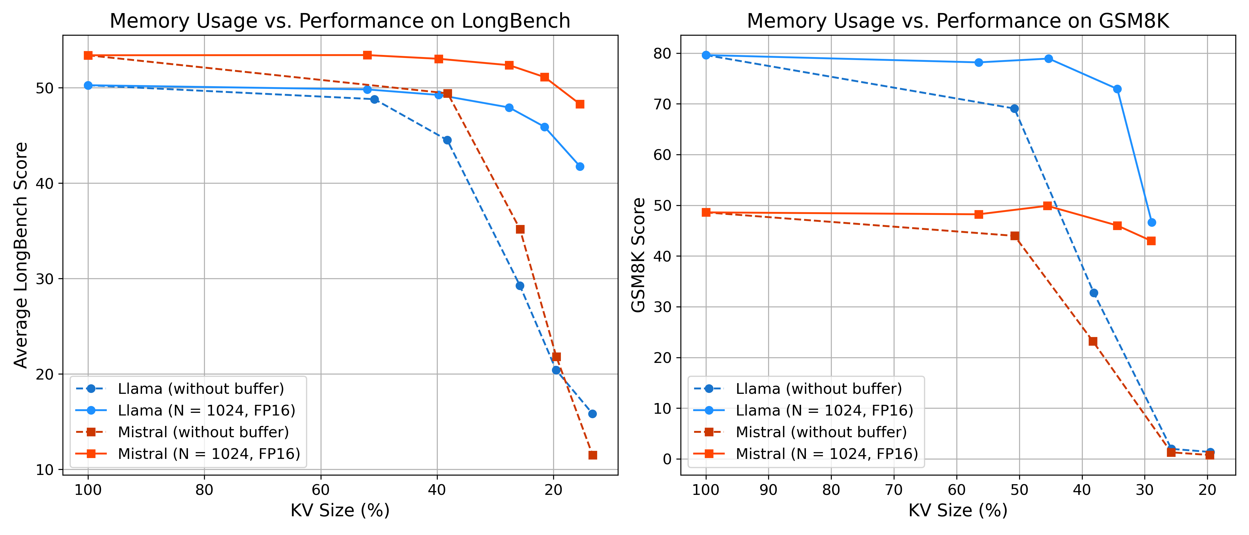
Figure 7: Memory usage vs. performance of Lexico with and without buffer on LongBench and GSM8K. The figure illustrates the impact of removing the buffer on the performance of Lexico when evaluated on the Llama-3.1-8B-Instruct and Mistral-7B-Instruct models for LongBench (left) and GSM8K (right) tasks. Solid lines represent configurations with a buffer, while dashed lines represent configurations without a buffer. We use a dictionary size of $N=1024$ and FP16 precision for the values of CSR tensors to vary sparsity and explore a wide range of KV sizes.

4.2.4 Adaptive Dictionary Learning

While our universal dictionaries demonstrate strong performance, we explore an adaptive learning method to better incorporate input-specific context. This adaptive approach improves performance by adding new dictionary atoms during generation when the predefined reconstruction error threshold is not met. These atoms, tailored to the input prompt, improve performance, but cannot be shared across batches, which requires them to be included in the KV size calculation. Although this approach boosts accuracy, it increases memory usage, limiting its ability to achieve low-memory regimes.

Though we observe some degree of universality in our dictionaries, as shown in Table 1, their performance is particularly strong on WikiText-103, the dataset they were trained on. To better incorporate input context information, we propose an extension that adaptively learns the dictionary during generation.

In this framework, we begin with a pre-trained universal dictionary as the initial dictionary. If, during the generation process, the sparse approximation fails to meet the predefined relative reconstruction error threshold, the problematic uncompressed key or value vector is normalized and added to the dictionary. The sparse representation of this vector is then stored with a sparsity of $s=1$, where its index corresponds to the newly added atom and its value is the $\ell_{2}$ norm of the uncompressed vector. The updated dictionary is subsequently used for further sparse approximations during the generation task. In this way, the adaptive learning framework incrementally refines the dictionaries, tailoring them to the specific generative task and enhancing overall performance at the cost of additional memory usage.

In our experiment, we initialize with a dictionary of size 1024 derived from WikiText-103; we then incorporate up to 1024 additional atoms during inference, resulting in a total dictionary size of $N=2048$. The maximum sparsity of $s=16$ is used, with a buffer size of $n_{b}=128$, and FP16 precision for the values of the CSR tensors. Results of this experiment are presented in Table 6. For both the Llama-3.1-8B-Instruct and Mistral-7B-Instruct models, the best GSM8K scores were observed when the relative reconstruction error threshold was set to $\delta=0.3$. Under this setting, the adaptive Lexico achieved improvements of $4.5\%p$ and $2.1\%p$ in the GSM8K score compared to the baseline Lexico for the Llama and Mistral models, respectively. The baseline Lexico uses a static initial dictionary of size 1024 without any adaptation. However, these improvements come at the cost of increased KV cache sizes of $9.1\%$ for Llama and $6.9\%$ for Mistral.

Table 6: GSM8K performance of adaptive Lexico. The table shows the GSM8K performance and KV cache sizes of adaptive Lexico on the Llama-3.1-8B-Instruct and Mistral-7B-Instruct-v0.3 models at varying reconstruction error thresholds ($\delta$). A universal dictionary of size 1024 is used, with up to 1024 additional atoms added during generation. The maximum sparsity of $s=16$, buffer size of $n_{b}=128$, and FP16 precision for CSR tensor values are applied.

Threshold ($\delta$)	Llama-3.1-8B-Instruct		Mistral-7B-Instruct-v0.3
	KV Size	GSM8K Score	KV Size	GSM8K Score
Full Cache	$100\%$	$79.61$	$100\%$	$48.60$
w/o Adaptation	$34.4\%$	$72.93$	$34.4\%$	$46.02$
$0.25$	n/a	n/a	$42.1\%$	$48.07$
$0.30$	$43.5\%$	$\mathbf{77.41}$	$41.3\%$	$\mathbf{48.14}$
$0.35$	$42.0\%$	$76.80$	$39.8\%$	$47.76$

4.3 Latency Analysis

In this section, we present latency measurements of the forward pass and OMP portion of Lexico during decoding stage in Table 7. We run simple generation tests on a 1000 token input to Llama-3.1-8B-Instruct model and generate up to 250 tokens to measure and aggregate latency metrics. We compare both dictionary sizes $N=1024$ and $4096$, which primarily affects OMP computation time. We set the sparsity level to $s=24$, and process OMP in batches of $n_{a}=8$.

Although we list the forward pass and OMP separately, the processes are implemented to run in parallel such that the one generation step takes the maximum of the two durations plus some overhead. However, with parallelization, there exists a time versus space complexity tradeoff, since running OMP also consumes GPU memory.

Higher latency of Lexico may be a limitation for latency-critical use cases. However, our primary focus is addressing highly memory-constrained scenarios. Such scenarios are increasingly critical for real-world LLM deployments, where even a batch size of one can exceed the capacity of a single GPU. By prioritizing memory efficiency, Lexico enables feasible deployment in contexts where other methods may encounter out-of-memory errors, offering a crucial contribution to memory-limited settings.

Table 7: Latency measurements. The following latencies measure the total time it takes for the respective computation to process when generating one new token. We use Llama-3.1-8B-Instruct and sum up the time each operation takes in total across all 32 layers. Latencies when dictionary sizes are 1024 and 4096 are measured. Detailed settings are described in Section 4.3.

Computation Type	Latency (per token)
-	$N=1024$	$N=4096$
Standard forward pass $({\bm{q}}{\bm{K}}^{\top})$	$48.39$ ms	–
Lexico: forward pass using ${\bm{q}}({\bm{K}}_{\text{csr}}{\bm{D}}_{k}^{\top})^{\top}$	$55.56$ ms	$56.35$ ms
Lexico: sparse approximation via OMP	$26.57$ ms	$40.58$ ms

5 Conclusion

In conclusion, our proposed method, Lexico, offers a novel approach to compressing KV cache for transformers by leveraging low-dimensional structures and sparse dictionary learning. Through this method, we demonstrate that substantial redundancy exists among key cache across various inputs, allowing us to compress the KV cache efficiently while maintaining near-lossless performance. Furthermore, Lexico enables compression rates that surpass traditional quantization techniques, offering fine-grained and wide control over memory usage. Importantly, our universal dictionary is both compact and scalable, making it applicable across tasks and user inputs without increasing memory demands. This approach provides strong memory savings, particularly for long-context tasks, by alleviating the memory bottlenecks associated with KV cache storage without dropping any previous tokens.

Future research directions based on our work include optimizing CSR tensors through customized quantizations and improving latency tradeoffs that occur due to the use of OMP during prefilling and decoding. It would also be interesting to apply “soft-eviction strategies” for sparse tensors in which sparsity level $s$ is determined or dropped later on based on the estimated importance of the token. A dynamic allocation of sparsity can further improve our compression method.

Appendix

Appendix A Implementation Details

Algorithm 1 illustrates a naive implementation of OMP for understanding. In Lexico, we adopt the implementation of OMP v0 proposed by (Zhu et al., 2020), which minimizes computational complexity using efficient inverse Cholesky factorization. Additionally, we integrate methods from (Lubonja et al., 2024) for batched GPU execution and extend the implementation to handle multiple dictionaries in parallel. Algorithm 2 presents the pseudocode for Lexico during the prefilling and decoding stages.

Algorithm 1 OMP

1:Signal ${\bm{k}}\in\mathbb{R}^{m}$, dictionary ${\bm{D}}\in\mathbb{R}^{m\times N}$, sparsity $s$

2:Sparse representation ${\bm{y}}\in\mathbb{R}^{n}$

3:Initialize ${\bm{r}}^{(0)}\leftarrow{\bm{k}}$, ${\mathbb{I}}^{(0)}\leftarrow\emptyset$, ${\bm{y}}^{(0)}\leftarrow\mathbf{0}$

4:for $i=1$ to $s$ do

5:     $n^{(i)}\leftarrow\arg\max_{1\leq n\leq N}\left\{\left|\left({\bm{D}}^{\top}\left({\bm{k}}-{\bm{D}}{\bm{y}}^{(i)}\right)\right)_{n}\right|\right\}$

6:     ${\mathbb{I}}^{(i)}\leftarrow{\mathbb{I}}^{(i-1)}\cup\left\{n^{(i)}\right\}$

7:     ${\bm{y}}^{(i+1)}\leftarrow\arg\min_{{\bm{y}}\in{\mathbb{R}}^{N}}\left\{\left\|{\bm{k}}-{\bm{D}}{\bm{y}}\right\|_{2},\text{Supp}\left({\bm{y}}\right)\subset{\mathbb{I}}^{(i)}\right\}$

8:end for

9:return ${\bm{y}}$

Algorithm 2 Prefilling and decoding with Lexico

1:Parameter: sparsity $s$, buffer length $n_{b}$, approximation length $n_{a}$

2:

3:procedure Prefilling

4:     Input: ${\bm{X}}\in\mathbb{R}^{l_{\text{seq}}\times d}$

5:     ${\bm{K}}\leftarrow{\bm{X}}{\bm{W}}_{k}$, ${\bm{V}}\leftarrow{\bm{X}}{\bm{W}}_{v}$

6:     ${\bm{K}}_{\text{csr}}\leftarrow\text{OMP}\left({\bm{K}}\left[:l_{\text{seq}}-n_{b}\right],{\bm{D}}_{k},s\right)$

7:     ${\bm{V}}_{\text{csr}}\leftarrow\text{OMP}\left({\bm{V}}\left[:l_{\text{seq}}-n_{b}\right],{\bm{D}}_{v},s\right)$

8:     ${\bm{K}}_{\text{buffer}}\leftarrow{\bm{K}}\left[l_{\text{seq}}-n_{b}:\right]$, ${\bm{V}}_{\text{buffer}}\leftarrow{\bm{V}}\left[l_{\text{seq}}-n_{b}:\right]$

9:     $\text{KV cache}\leftarrow{\bm{K}}_{\text{csr}},{\bm{K}}_{\text{buffer}},{\bm{V}}_{\text{csr}},{\bm{V}}_{\text{buffer}}$

10:     return ${\bm{K}}$, ${\bm{V}}$

11:end procedure

12:

13:procedure Decoding

14:     Input: KV cache, ${\bm{x}}_{t}\in\mathbb{R}^{1\times d}$

15:     ${\bm{q}}_{t}\leftarrow{\bm{x}}_{t}{\bm{W}}_{q}$, ${\bm{k}}_{t}\leftarrow{\bm{x}}_{t}{\bm{W}}_{k}$, ${\bm{v}}_{t}\leftarrow{\bm{x}}_{t}{\bm{W}}_{v}$

16:     ${\bm{K}}_{\text{csr}},{\bm{K}}_{\text{buffer}},{\bm{V}}_{\text{csr}},{\bm{V}}_{\text{buffer}}\leftarrow\text{KV cache}$

17:     ${\bm{K}}_{\text{buffer}}\leftarrow\text{Concat}\left(\left[{\bm{K}}_{\text{buffer}},{\bm{k}}_{t}\right],\text{dim}=\text{token}\right)$

18:     ${\bm{V}}_{\text{buffer}}\leftarrow\text{Concat}\left(\left[{\bm{V}}_{\text{buffer}},{\bm{v}}_{t}\right],\text{dim}=\text{token}\right)$

19:     ${\bm{a}}_{t}\leftarrow\text{Concat}\left(\left[{\bm{q}}_{t}{\bm{D}}_{k}{\bm{K}}_{\text{csr}},{\bm{q}}_{t}{\bm{K}}_{\text{buffer}}\right],\text{dim}=\text{token}\right)$

20:     ${\bm{a}}_{t}\leftarrow\text{Softmax}\left({\bm{a}}_{t}\right)$

21:     ${\bm{V}}\leftarrow\text{Concat}\left(\left[{\bm{D}}_{v}{\bm{V}}_{\text{csr}},{\bm{V}}_{\text{buffer}}\right],\text{dim}=\text{token}\right)$

22:     ${\bm{o}}_{t}\leftarrow{\bm{a}}_{t}{\bm{V}}$

23:     if $\text{len}\left({\bm{K}}_{\text{buffer}}\right)>n_{b}$ then

24:         ${{\bm{K}}^{\prime}}_{\text{csr}}\leftarrow\text{OMP}\left({\bm{K}}_{\text{buffer}}\left[:n_{a}\right],{\bm{D}}_{k},s\right)$

25:         ${{\bm{V}}^{\prime}}_{\text{csr}}\leftarrow\text{OMP}\left({\bm{V}}_{\text{buffer}}\left[:n_{a}\right],{\bm{D}}_{v},s\right)$

26:         ${\bm{K}}_{\text{csr}}\leftarrow\text{Concat}\left(\left[{\bm{K}}_{\text{csr}},{{\bm{K}}^{\prime}}_{\text{csr}}\right],\text{dim}=\text{token}\right)$

27:         ${\bm{V}}_{\text{csr}}\leftarrow\text{Concat}\left(\left[{\bm{V}}_{\text{csr}},{{\bm{V}}^{\prime}}_{\text{csr}}\right],\text{dim}=\text{token}\right)$

28:         ${\bm{K}}_{\text{buffer}}\leftarrow{\bm{K}}_{\text{buffer}}\left[n_{a}:\right]$, ${\bm{V}}_{\text{buffer}}\leftarrow{\bm{V}}_{\text{buffer}}\left[n_{a}:\right]$

29:     end if

30:     $\text{KV cache}\leftarrow{\bm{K}}_{\text{csr}},{\bm{K}}_{\text{buffer}},{\bm{V}}_{\text{csr}},{\bm{V}}_{\text{buffer}}$

31:     return ${\bm{o}}_{t}$

32:end procedure

Appendix B LongBench Task Statistics

Table 8: Details of LongBench tasks used in experiments.

Task	Task Type	Evaluation Metric	Average Length	# of Samples
Qasper	Single-doc QA	F1	3619	200
QMSum	Summarization	ROUGE-L	10614	200
MultiNews	Summarization	ROUGE-L	2113	200
TREC	Few-shot information retrieval	Accuracy	5177	200
TriviaQA	Few-shot reading comprehension	F1	8209	200
SAMSum	Few-shot dialogue summarization	ROUGE-L	6258	200
LCC	Code completion	Edit Similarity	1235	500
RepoBench-P	Code completion	Edit Similarity	4206	500

Appendix C Ablation Study: Experimental Results

C.1 Performance without Buffer

In this section, we assess the effect of the buffer by comparing the results with and without its use. We illustrated the result in Figure 7 in Section 4.2.3. The quantitative results for LongBench and GSM8K are presented in Table 9 and Table 10, respectively.

Table 9: LongBench performance without buffer. This table shows the impact of removing the buffer of Lexico on the performance of the Llama-3.1-8B-Instruct and Mistral-7B-Instruct models at varying sparsity levels. A dictionary size of $N=1024$ and FP16 precision for the values of the CSR tensors are used.

Sparsity	KV Size	Qasper	QMSum	MultiNews	TREC	TriviaQA	SAMSum	LCC	RepoBench-P	Average
Llama-3.1-8B-Instruct
Full Cache	$100\%$	$13.10$	$23.46$	$26.94$	$72.5$	$91.65$	$43.47$	$63.15$	$56.76$	$48.88$
$s=32$	$50.8\%$	$14.87$	$26.51$	$26.57$	$71.5$	$92.48$	$42.88$	$61.54$	$54.04$	$48.80$
$s=24$	$38.2\%$	$13.37$	$25.02$	$22.54$	$65.0$	$91.75$	$39.71$	$52.21$	$46.48$	$44.51$
$s=16$	$25.8\%$	$8.27$	$13.74$	$10.70$	$54.5$	$77.51$	$20.45$	$26.53$	$22.46$	$29.27$
$s=12$	$19.5\%$	$6.31$	$10.15$	$5.66$	$39.0$	$53.70$	$6.83$	$22.18$	$19.46$	$20.41$
$s=8$	$13.3\%$	$2.74$	$8.05$	$4.17$	$36.5$	$34.45$	$4.27$	$18.24$	$18.32$	$15.84$
Mistral-7B-Instruct-v0.3
Full Cache	$100\%$	$41.58$	$25.69$	$27.76$	$76.0$	$88.59$	$47.58$	$59.37$	$60.60$	$53.40$
$s=32$	$50.8\%$	$40.27$	$25.21$	$27.53$	$76.5$	$89.01$	$45.77$	$58.64$	$59.07$	$52.75$
$s=24$	$38.2\%$	$37.46$	$24.41$	$27.34$	$75.5$	$88.66$	$43.87$	$48.55$	$49.50$	$49.41$
$s=16$	$25.8\%$	$25.57$	$18.49$	$15.19$	$71.5$	$81.91$	$27.90$	$19.39$	$21.45$	$35.18$
$s=12$	$19.5\%$	$18.59$	$13.11$	$5.95$	$58.0$	$50.13$	$2.86$	$13.38$	$12.60$	$21.83$
$s=8$	$13.3\%$	$10.32$	$6.98$	$2.67$	$31.5$	$20.01$	$2.27$	$10.18$	$8.11$	$11.51$

Table 10: GSM8K performance without buffer. This table shows the impact of removing the buffer of Lexico on the performance of the Llama-3.1-8B-Instruct and Mistral-7B-Instruct models at varying sparsity levels. A dictionary size of $N=1024$ and FP16 precision for the values of the CSR tensors are used.

Sparsity	KV Size	Llama-3.1-8B-Instruct	Mistral-7B-Instruct-v0.3
Full Cache	$100\%$	$79.61$	$48.60$
$s=32$	$50.8\%$	$69.07$	$43.97$
$s=24$	$38.2\%$	$32.75$	$23.20$
$s=16$	$25.8\%$	$1.97$	$1.29$
$s=12$	$19.6\%$	$1.36$	$0.76$

Appendix D Qualitative Results

D.1 GSM8K Example Generation

The boxes highlight the correct intermediate answers that must be derived. The highlighted colors in red show incorrect reasoning and answers. We provide the original problem and solution below, along with outputs from Llama-3.1-8B-Instruct with full KV cache (FP16), Lexico (sparsity $s=14$), and KIVI-2.

Original Problem & Solution

Problem: The Kennel house keeps 3 German Shepherds and 2 Bulldogs. If a German Shepherd consumes 5 kilograms of dog food and a bulldog consumes 3 kilograms of dog food per day, how many kilograms of dog food will they need in a week?

Solution: The German Shepherds consume $3\times 5=\boxed{15}$ kilograms of dog food per day.

The Bulldogs consume $2\times 3=\boxed{6}$ kilograms of dog food per day.

The dogs consume a total of $15+6=\boxed{21}$ kilograms of dog food per day.

Therefore, they need $21\times 7=\boxed{147}$ kilograms of dog food in a week.

Final Answer: 147

Llama-3.1-8B-Instruct with Full Cache

First, find the total amount of food the German Shepherds consume in a day: $3$ dogs $\times$ $5$ kg/dog $=15$ kg.

Then find the total amount of food the Bulldogs consume in a day: $2$ dogs $\times$ $3$ kg/dog $=6$ kg.

Add the two amounts together to find the total amount of food the dogs consume in a day: $15$ kg $+6$ kg $=21$ kg.

Multiply that number by 7 to find the total amount of food the dogs consume in a week: $21$ kg/day $\times 7$ days $=147$ kg.

Llama-3.1-8B-Instruct with Lexico ($s=14$)

The kennel has $3$ German Shepherds and $2$ Bulldogs, so they have $3+2=5$ dogs.

The German Shepherds consume $5\times 3=15$ kilograms of dog food per day.

The Bulldogs consume $2\times 3=6$ kilograms of dog food per day.

So, the kennel needs $15+6=21$ kilograms of dog food per day.

In a week, they will need $21\times 7=147$ kilograms of dog food.

The answer is 147.

Llama-3.1-8B-Instruct with KIVI-2

The Kennel house has $3$ German Shepherds and $2$ Bulldogs, so they have a total of $3+2=\boxed{5}$ dogs.

Each German Shepherd consumes $5$ kilograms of dog food per day, so the total amount of dog food consumed by the German Shepherds is $5\times 5=\boxed{25}$ kilograms per day.

Each Bulldog consumes $3$ kilograms of dog food per day, so the total amount of dog food consumed by the Bulldogs is $2\times 3=\boxed{6}$ kilograms per day.

The total amount of dog food consumed per day is $25+6=\boxed{31}$ kilograms.

The Kennel house will need $31\times 7=\boxed{217}$ kilograms of dog food in a week.

References

- Ainslie et al. (2023) Joshua Ainslie, James Lee-Thorp, Michiel de Jong, Yury Zemlyanskiy, Federico Lebron, and Sumit Sanghai. Gqa: Training generalized multi-query transformer models from multi-head checkpoints. In Proceedings of the 2023 Conference on Empirical Methods in Natural Language Processing, pp. 4895–4901, 2023.
- Bai et al. (2023) Yushi Bai, Xin Lv, Jiajie Zhang, Hongchang Lyu, Jiankai Tang, Zhidian Huang, Zhengxiao Du, Xiao Liu, Aohan Zeng, Lei Hou, et al. Longbench: A bilingual, multitask benchmark for long context understanding. arXiv preprint arXiv:2308.14508, 2023.
- Beltagy et al. (2020) Iz Beltagy, Matthew E Peters, and Arman Cohan. Longformer: The long-document transformer. arXiv preprint arXiv:2004.05150, 2020.
- Bricken et al. (2023) Trenton Bricken, Adly Templeton, Joshua Batson, Brian Chen, Adam Jermyn, Tom Conerly, Nick Turner, Cem Anil, Carson Denison, Amanda Askell, et al. Towards monosemanticity: Decomposing language models with dictionary learning. Transformer Circuits Thread, 2, 2023.
- Cai et al. (2024) Zefan Cai, Yichi Zhang, Bofei Gao, Yuliang Liu, Tianyu Liu, Keming Lu, Wayne Xiong, Yue Dong, Baobao Chang, Junjie Hu, et al. Pyramidkv: Dynamic kv cache compression based on pyramidal information funneling. arXiv preprint arXiv:2406.02069, 2024.
- Candès et al. (2006) Emmanuel J Candès, Justin Romberg, and Terence Tao. Robust uncertainty principles: Exact signal reconstruction from highly incomplete frequency information. IEEE Transactions on information theory, 52(2):489–509, 2006.
- Cobbe et al. (2021) Karl Cobbe, Vineet Kosaraju, Mohammad Bavarian, Mark Chen, Heewoo Jun, Lukasz Kaiser, Matthias Plappert, Jerry Tworek, Jacob Hilton, Reiichiro Nakano, et al. Training verifiers to solve math word problems. arXiv preprint arXiv:2110.14168, 2021.
- Dai et al. (2024) Damai Dai, Chengqi Deng, Chenggang Zhao, RX Xu, Huazuo Gao, Deli Chen, Jiashi Li, Wangding Zeng, Xingkai Yu, Y Wu, et al. Deepseekmoe: Towards ultimate expert specialization in mixture-of-experts language models. arXiv preprint arXiv:2401.06066, 2024.
- Devoto et al. (2024) Alessio Devoto, Yu Zhao, Simone Scardapane, and Pasquale Minervini. A simple and effective norm-based strategy for kv cache compression. arXiv preprint arXiv:2406.11430, 2024.
- Dong et al. (2024) Harry Dong, Xinyu Yang, Zhenyu Zhang, Zhangyang Wang, Yuejie Chi, and Beidi Chen. Get more with less: Synthesizing recurrence with kv cache compression for efficient llm inference. In Forty-first International Conference on Machine Learning, 2024.
- Dong et al. (2014) Weisheng Dong, Guangming Shi, Xin Li, Yi Ma, and Feng Huang. Compressive sensing via nonlocal low-rank regularization. IEEE transactions on image processing, 23(8):3618–3632, 2014.
- Donoho (2006) David L Donoho. Compressed sensing. IEEE Transactions on information theory, 52(4):1289–1306, 2006.
- Ge et al. (2023) Suyu Ge, Yunan Zhang, Liyuan Liu, Minjia Zhang, Jiawei Han, and Jianfeng Gao. Model tells you what to discard: Adaptive kv cache compression for llms. In The Twelfth International Conference on Learning Representations, 2023.
- He et al. (2024) Yefei He, Luoming Zhang, Weijia Wu, Jing Liu, Hong Zhou, and Bohan Zhuang. Zipcache: Accurate and efficient kv cache quantization with salient token identification. arXiv preprint arXiv:2405.14256, 2024.
- Hooper et al. (2024) Coleman Hooper, Sehoon Kim, Hiva Mohammadzadeh, Michael W Mahoney, Yakun Sophia Shao, Kurt Keutzer, and Amir Gholami. Kvquant: Towards 10 million context length llm inference with kv cache quantization. arXiv preprint arXiv:2401.18079, 2024.
- Kang et al. (2024) Hao Kang, Qingru Zhang, Souvik Kundu, Geonhwa Jeong, Zaoxing Liu, Tushar Krishna, and Tuo Zhao. Gear: An efficient kv cache compression recipefor near-lossless generative inference of llm. arXiv preprint arXiv:2403.05527, 2024.
- Kingma & Ba (2014) Diederik P Kingma and Jimmy Ba. Adam: A method for stochastic optimization. arXiv preprint arXiv:1412.6980, 2014.
- Kwon et al. (2023) Woosuk Kwon, Zhuohan Li, Siyuan Zhuang, Ying Sheng, Lianmin Zheng, Cody Hao Yu, Joseph Gonzalez, Hao Zhang, and Ion Stoica. Efficient memory management for large language model serving with pagedattention. In Proceedings of the 29th Symposium on Operating Systems Principles, pp. 611–626, 2023.
- Li et al. (2024) Yuhong Li, Yingbing Huang, Bowen Yang, Bharat Venkitesh, Acyr Locatelli, Hanchen Ye, Tianle Cai, Patrick Lewis, and Deming Chen. Snapkv: Llm knows what you are looking for before generation. arXiv preprint arXiv:2404.14469, 2024.
- Lin et al. (2024) Bin Lin, Tao Peng, Chen Zhang, Minmin Sun, Lanbo Li, Hanyu Zhao, Wencong Xiao, Qi Xu, Xiafei Qiu, Shen Li, et al. Infinite-llm: Efficient llm service for long context with distattention and distributed kvcache. arXiv preprint arXiv:2401.02669, 2024.
- Liu et al. (2024a) Zichang Liu, Aditya Desai, Fangshuo Liao, Weitao Wang, Victor Xie, Zhaozhuo Xu, Anastasios Kyrillidis, and Anshumali Shrivastava. Scissorhands: Exploiting the persistence of importance hypothesis for llm kv cache compression at test time. Advances in Neural Information Processing Systems, 36, 2024a.
- Liu et al. (2024b) Zirui Liu, Jiayi Yuan, Hongye Jin, Shaochen Zhong, Zhaozhuo Xu, Vladimir Braverman, Beidi Chen, and Xia Hu. Kivi: A tuning-free asymmetric 2bit quantization for kv cache. arXiv preprint arXiv:2402.02750, 2024b.
- Lubonja et al. (2024) Ariel Lubonja, Sebastian Kazmarek Præsius, and Trac Duy Tran. Efficient batched cpu/gpu implementation of orthogonal matching pursuit for python. arXiv preprint arXiv:2407.06434, 2024.
- Makhzani & Frey (2013) Alireza Makhzani and Brendan Frey. K-sparse autoencoders. arXiv preprint arXiv:1312.5663, 2013.
- Merity (2016) Stephen Merity. The wikitext long term dependency language modeling dataset. Salesforce Metamind, 9, 2016.
- Metzler et al. (2016) Christopher A Metzler, Arian Maleki, and Richard G Baraniuk. From denoising to compressed sensing. IEEE Transactions on Information Theory, 62(9):5117–5144, 2016.
- Qin et al. (2024) Ruoyu Qin, Zheming Li, Weiran He, Mingxing Zhang, Yongwei Wu, Weimin Zheng, and Xinran Xu. Mooncake: A kvcache-centric disaggregated architecture for llm serving, 2024. arXiv preprint arxiv:2407.00079, 2024.
- Shazeer (2019) Noam Shazeer. Fast transformer decoding: One write-head is all you need. arXiv preprint arXiv:1911.02150, 2019.
- Singhania et al. (2024) Prajwal Singhania, Siddharth Singh, Shwai He, Soheil Feizi, and Abhinav Bhatele. Loki: Low-rank keys for efficient sparse attention. arXiv preprint arXiv:2406.02542, 2024.
- Sun et al. (2024) Yutao Sun, Li Dong, Yi Zhu, Shaohan Huang, Wenhui Wang, Shuming Ma, Quanlu Zhang, Jianyong Wang, and Furu Wei. You only cache once: Decoder-decoder architectures for language models. arXiv preprint arXiv:2405.05254, 2024.
- Vaswani et al. (2017) Ashish Vaswani, Noam Shazeer, Niki Parmar, Jakob Uszkoreit, Llion Jones, Aidan N Gomez, Lukasz Kaiser, and Illia Polosukhin. Attention is all you need. In Advances in Neural Information Processing Systems 30: Annual Conference on Neural Information Processing Systems 2017, pp. 5998–6008, 2017.
- Wang et al. (2024a) Yubo Wang, Xueguang Ma, Ge Zhang, Yuansheng Ni, Abhranil Chandra, Shiguang Guo, Weiming Ren, Aaran Arulraj, Xuan He, Ziyan Jiang, et al. Mmlu-pro: A more robust and challenging multi-task language understanding benchmark. arXiv preprint arXiv:2406.01574, 2024a.
- Wang et al. (2024b) Zheng Wang, Boxiao Jin, Zhongzhi Yu, and Minjia Zhang. Model tells you where to merge: Adaptive kv cache merging for llms on long-context tasks. arXiv preprint arXiv:2407.08454, 2024b.
- Xiao et al. (2023) Guangxuan Xiao, Yuandong Tian, Beidi Chen, Song Han, and Mike Lewis. Efficient streaming language models with attention sinks. In The Twelfth International Conference on Learning Representations, 2023.
- Ye et al. (2024) Lu Ye, Ze Tao, Yong Huang, and Yang Li. Chunkattention: Efficient self-attention with prefix-aware kv cache and two-phase partition. arXiv preprint arXiv:2402.15220, 2024.
- Yu et al. (2022) Gyeong-In Yu, Joo Seong Jeong, Geon-Woo Kim, Soojeong Kim, and Byung-Gon Chun. Orca: A distributed serving system for Transformer-Based generative models. In 16th USENIX Symposium on Operating Systems Design and Implementation (OSDI 22), pp. 521–538, 2022.
- Yu et al. (2024) Hao Yu, Zelan Yang, Shen Li, Yong Li, and Jianxin Wu. Effectively compress kv heads for llm. arXiv preprint arXiv:2406.07056, 2024.
- Yue et al. (2024) Yuxuan Yue, Zhihang Yuan, Haojie Duanmu, Sifan Zhou, Jianlong Wu, and Liqiang Nie. Wkvquant: Quantizing weight and key/value cache for large language models gains more. arXiv preprint arXiv:2402.12065, 2024.
- Zhang et al. (2024) Zhenyu Zhang, Ying Sheng, Tianyi Zhou, Tianlong Chen, Lianmin Zheng, Ruisi Cai, Zhao Song, Yuandong Tian, Christopher Ré, Clark Barrett, et al. H2o: Heavy-hitter oracle for efficient generative inference of large language models. Advances in Neural Information Processing Systems, 36, 2024.
- Zhu et al. (2020) Hufei Zhu, Wen Chen, and Yanpeng Wu. Efficient implementations for orthogonal matching pursuit. Electronics, 9(9):1507, 2020.