A SPectroscopic survey of biased halos In the Reionization Era (ASPIRE):
Spectroscopically Complete Census of Obscured Cosmic Star Formation Rate Density at $z=4-6$

Abstract

We present a stringent measurement of the dust-obscured star-formation rate density (SFRD) at $z=4-6$ from the ASPIRE JWST Cycle-1 medium and ALMA Cycle-9 large program. We obtained JWST/NIRCam grism spectroscopy and ALMA 1.2-mm continuum map along 25 independent quasar sightlines, covering a total survey area of $\sim$35 arcmin² where we search for dusty star-forming galaxies (DSFGs) at $z=0-7$. We identify eight DSFGs in seven fields at $z=4-6$ through the detection of H$\alpha$ or [O III] $\lambda$5008 lines, including fainter lines such as H$\beta$, [O III] $\lambda$4960, [N II] $\lambda$6585, [S II] $\lambda\lambda$6718,6733 for six sources. With this spectroscopically complete DSFG sample at $z=4-6$ and negligible impact from cosmic variance (shot noise), we measure the infrared luminosity function (IRLF) down to $L_{\mathrm{IR}}\sim 2\times 10^{11}$ $\mathrm{L}_{\odot}$. We find flattening of IRLF at $z=4-6$ towards the faint end (power-law slope $\alpha=0.59_{-0.45}^{+0.39}$). We determine the dust-obscured cosmic SFRD at this epoch as $\log[\rho_{\mathrm{SFR,IR}}/(\mathrm{M}_{\odot}\,\mathrm{yr}^{-1}\,\mathrm{Mpc}^{-3})]=-1.52_{-0.13}^{+0.14}$. This is significantly higher than previous determination using ALMA data in the Hubble Ultra Deep Field, which is void of DSFGs at $z=4-6$ because of strong cosmic variance (shot noise). We conclude that the majority ($66\pm 7$%) of cosmic star formation at $z\sim 5$ is still obscured by dust. We also discuss the uncertainty of SFRD propagated from far-IR spectral energy distribution and IRLF at the bright end, which will need to be resolved with future ALMA and JWST observations.

tablenum SIXtablenum

1 Introduction

It is now clear that the cosmic star formation history peaked at around a redshift of two (see review by Madau & Dickinson 2014). Before this so-called “cosmic noon”, a decline of unobscured cosmic star formation rate densities (SFRD) toward higher redshifts has been suggested by Hubble Space Telescope (HST) observations at rest-frame ultraviolet (UV) wavelength (e.g., Bouwens et al., 2015, 2020; Finkelstein et al., 2015). However, the measurements of dust-obscured SFRD at infrared (IR) to millimeter wavelengths were much more challenging and uncertain. Although exciting constraints have been placed with multiple telescopes including Herschel (e.g., Burgarella et al., 2013; Gruppioni et al., 2013; Rowan-Robinson et al., 2016; Liu et al., 2018; Wang et al., 2019a), James Clerk Maxwell Telescope (JCMT; e.g., Koprowski et al. 2017; Lim et al. 2020) and Atacama Large Millimeter/submillimeter Array (ALMA; e.g., Dunlop et al., 2017; Bouwens et al., 2020; Gruppioni et al., 2020; Khusanova et al., 2021; Zavala et al., 2021; Fujimoto et al., 2023; Magnelli et al., 2024; Traina et al., 2024), most of existing studies rely on a long list of assumptions, including the shape of infrared luminosity function (IRLF), mid-to-far-IR spectral energy distribution (SED), and also photometric redshifts that are strongly degenerate with the stellar age and dust attenuation.

One of the most critical uncertainties is from photometric redshifts ($z_{\mathrm{phot}}$). The vast majority of dusty star-forming galaxies (DSFGs) are found at $z\simeq 2-3$ (e.g., see reviews by Casey et al., 2014a; Hodge & da Cunha, 2020). Therefore, it is usually very challenging to differentiate true DSFGs at $z>4$ from lower-redshift “interlopers” with large $z_{\mathrm{phot}}$ error (e.g., see the recent dispute of COSBO-7 at $z_{\mathrm{phot}}$ $>$ 7 but spectroscopic redshift $z_{\mathrm{spec}}$ $=$ 2.625; Ling et al. 2024, Jin et al. 2024a). Many of these DSFGs at $z_{\mathrm{phot}}$ $\gtrsim$ 4 are totally dust-obscured at HST wavelengths, and therefore also known as “HST-dark”, “NIR-dark”, “$H$-dropout” or “$H$-faint” galaxies (e.g., Huang et al., 2011; da Cunha et al., 2015; Simpson et al., 2015; Fujimoto et al., 2016; Franco et al., 2018; Alcalde Pampliega et al., 2019; Wang et al., 2019b; Yamaguchi et al., 2019; Sun et al., 2021; Talia et al., 2021; Enia et al., 2022; Gómez-Guijarro et al., 2022; Kokorev et al., 2022; Manning et al., 2022; Xiao et al., 2023b; Tsujita et al., 2024), including certain amount of galaxies that are only detected with ALMA (e.g., Decarli et al., 2017; Mazzucchelli et al., 2019; Venemans et al., 2019; Williams et al., 2019; Fudamoto et al., 2021; Wang et al., 2023). Therefore, it is very challenging to obtain secure redshifts of these galaxies through ground-based optical/near-IR spectroscopy.

At $z\gtrsim 4$, luminous infrared galaxies (LIRG; IR luminosity $10^{11}\,\mbox{$\mathrm{L}_{\odot}$}\leq L_{\mathrm{IR}}<10^{12}$ $\mathrm{L}_{\odot}$) and the bulk of ultra-luminous infrared galaxies (ULIRG; $10^{12}\,\mbox{$\mathrm{L}_{\odot}$}\leq L_{\mathrm{IR}}<10^{13}$ $\mathrm{L}_{\odot}$) are below the Herschel/SPIRE confusion noise limit at 250–500 $\mathrm{\SIUnitSymbolMicro m}$ (e.g., Nguyen et al., 2010), making it difficult to tightly constrain redshifts through far-IR SED except for extraordinarily luminous and/or gravitationally lensed galaxies (e.g., Riechers et al., 2013; Rawle et al., 2014; Sun et al., 2022). Large millimeter interferometers (e.g., ALMA, Plateau de Bure Interferometer, PdBI and its successor, Northern Extended Millimeter Array, NOEMA) can obtain redshifts of distant DSFGs through CO and [C II] $\lambda$158 $\mathrm{\SIUnitSymbolMicro m}$ line scans. However, such type of observations are time-consuming for high-redshift LIRGs and ULIRGs (e.g., 8.3-hour on-source for the ALMA CO scan of MAMBO-9 at $z_{\mathrm{spec}}$ $=$ 5.85 with $L_{\mathrm{IR}}$ $\sim$ $4\times 10^{12}$ $\mathrm{L}_{\odot}$; Casey et al. 2019; Jin et al. 2019b), with again exceptions for extraordinarily luminous sources at observed $L_{\mathrm{IR}}$ $\gtrsim$ $10^{13}$ $\mathrm{L}_{\odot}$ (e.g., Weiß et al., 2013; Strandet et al., 2016; Reuter et al., 2020; Chen et al., 2022).

Without spectroscopic redshifts, it is very challenging to securely select a sample of DSFGs at $z>4$, directly measure their IRLF and accurately determine the obscured SFRD. For example, based on serendipitous (sub-)millimeter continuum sources discovered by Cycle-5 “ALMA Large Program to INvestigate CII at Early Times” (ALPINE, Le Fèvre et al. 2020), Gruppioni et al. (2020) found that the obscured SFRD remains almost constant across $z\simeq 2-6$. This is in great contrast to the results based on Cycle-4 large program “ALMA Spectroscopic Survey in the Hubble Ultra Deep Field (HUDF)” (ASPECS; Walter et al. 2016), where no DSFGs at $z>4$ was blindly discovered with deep 1-mm and 3-mm survey of the HUDF (Aravena et al. 2020; also Dunlop et al. 2017; Hatsukade et al. 2018). Alternative methods have been developed to infer obscured SFRD through the relation between infrared excess (IRX = $L_{\mathrm{IR}}/L_{\mathrm{UV}}$, i.e., IR-to-UV luminosity ratio) and UV continuum slope $\beta_{\mathrm{UV}}$ (e.g., Meurer et al., 1999) or stellar mass $M_{\mathrm{star}}$ (e.g., Bouwens et al., 2020; Khusanova et al., 2021; Algera et al., 2023; Magnelli et al., 2024), or a backward modeling approach that could infer the redshift evolution of IRLF (and thus obscured SFRD) through (sub)-millimeter number counts (Casey et al., 2018b, a; Zavala et al., 2021). Nevertheless, the obscured SFRD at $z\sim 5$ measured based on ASPECS (e.g., Bouwens et al., 2020; Zavala et al., 2021) data is still lower than that measured with ALPINE by $\sim$ 1 dex (Gruppioni et al., 2020).

Most recently, direct measurements through ALMA Cycle-6 large program “ALMA Lensing Cluster Survey” (ALCS; Kohno et al., 2023) suggest that the obscured SFRD at $z\sim 5$ is between those inferred through ALPINE and ASPECS programs (Fujimoto et al., 2023). Despite significant advance made with ALCS in probing DSFGs towards sub-LIRG-luminosity ($L_{\mathrm{IR}}$ $<$ $10^{11}$ $\mathrm{L}_{\odot}$) and reducing cosmic variance (shot noise) through 33 lensing cluster fields, caution is still necessary as the ALCS sample of DSFGs at $z>4$ is not yet spectroscopically complete.

JWST (Gardner et al., 2023) provides unprecedented opportunities to obtain near-IR spectroscopy of DSFGs at high redshifts. Specifically, with NIRCam wide-field slitless spectroscopy (WFSS) at 2.4–5.0 $\mathrm{\SIUnitSymbolMicro m}$ (Rieke et al., 2023), it is now possible to obtain near-IR spectra of all galaxies that enter the field of view (FoV; up to $\sim$ 9 arcmin²). It has been clear from JWST Cycle-1 programs that H$\alpha$ lines from HST-dark DSFGs at $z>5$ can be easily detected with NIRCam WFSS with an on-source integration time of 1–2 hours (e.g., Herard-Demanche et al., 2023; Sun et al., 2024; Williams et al., 2024; Xiao et al., 2023a). This promises a highly complete spectroscopic survey of dust-obscured star formation history towards the Epoch of Reionization.

In this work, we present a stringent measurement of IRLF and obscured SFRD at $z=4-6$ through the ASPIRE JWST Cycle-1 medium and ALMA Cycle-9 large program (Wang, F. et al. in prep.). Through ALMA and JWST spectroscopic survey of DSFGs over 25 independent quasar sightlines, we discovered eight DSFGs at $z_{\mathrm{spec}}=4-6$ down to 1.2-mm flux density of $S_{\mathrm{1.2mm}}\sim 0.15$ mJy. We describe the observations and data processing techniques in Section 2, present the redshift confirmation and analyses of their physical properties in Section 3. We then study their dust obscuration, contribution to 1.2–mm number count, IRLF and obscured SFRD in Section 4. Further implications and cautions are discussed in Section 5. Our conclusions are summarized in Section 6.

Throughout this work, we assume a flat $\Lambda$CDM cosmology with $H_{0}=70$ $\mathrm{k}\mathrm{m}\,\mathrm{s}^{-1}\,\mathrm{M}\mathrm{p}\mathrm{c}^{-1}$, $\Omega_{\mathrm{M}}=0.3$ and $\sigma_{8}=0.8$. AB magnitude system (Oke & Gunn, 1983) is adopted to describe source brightness in the optical and near-IR. We also assume a Chabrier (2003) initial mass function. We define the IR luminosity ($L_{\mathrm{IR}}$) as the integrated luminosity over a rest-frame wavelength range from 8 to 1000 $\mathrm{\SIUnitSymbolMicro m}$.

2 Observation and Data Reduction

2.1 JWST/NIRCam

A SPectroscopic survey of biased halos In the Reionization Era (ASPIRE) started as a 62-hour JWST Cycle-1 medium program (PI: Wang, F.; Program ID: 2078). With the powerful NIRCam WFSS observing mode, ASPIRE observed 25 luminous quasars at $z=6.5-6.8$ through NIRCam grism WFSS in the F356W filter (3.1–4.0 $\mathrm{\SIUnitSymbolMicro m}$) and imaging in the F115W, F200W and F356W filter (1–4 $\mathrm{\SIUnitSymbolMicro m}$). The observational design of ASPIRE JWST program will be presented by Wang, F. et al. (in prep.; see also Wang et al. 2023; Yang et al. 2023). The primary science goal of ASPIRE is to detect companion galaxies at the quasar redshifts through [O III] $\lambda\lambda$4960,5008 and H$\beta$ lines, and therefore answer whether the most massive black holes in the early Universe reside in the most massive dark matter halos (Wang et al., 2023). ASPIRE has also enabled a large number of other scientific investigations including supermassive black hole mass measurements (Yang et al., 2023), morphology of quasar host galaxies and outflows (Yang, J. et al. in prep.), the environmental impact on galaxy properties and evolution history at $z\sim 6.5$ (Champagne et al., 2024a, b), the connection between intergalactic medium (IGM) opacity and galaxies at $z\sim 6$ (Jin et al., 2024b), and the metal enrichment of circumgalactic medium (CGM) at $z\simeq 4-6$ (Wu et al., 2023; Zou et al., 2024).

In all of the 25 quasar fields observed with ASPIRE, the NIRCam WFSS on-source integration time with the F356W filter is 2834 s. Grism R was used, which disperses light along the row (horizontal) direction of the detector at a spectral resolution of $R\simeq 1300-1600$. The quasar was placed in the full spectral coverage region in module A (see Wang et al. 2023 and Figure 1) because of higher throughput (Rieke et al., 2023). During the NIRCam WFSS exposure through the long-wavelength (LW) channel, the short-wavelength (SW) channel of NIRCam obtained direct imaging observation with the F200W filter. After the WFSS exposure, direct imaging observations were obtained in F115W and F356W filter through SW and LW channel, respectively, and the exposure time is 1417 s for both filters.

ASPIRE NIRCam data reduction has been described by Wang et al. (2023) and Yang et al. (2023) and will be described in full details by Wang, F. et al. (in prep.). Here we only briefly described the key steps adopted in the data processing routine.

The NIRCam imaging data were processed based on jwst calibration pipeline (Bushouse et al., 2023) v1.10.2 with the reference files jwst_1080.pmap (including JWST Cycle-1 NIRCam flux calibrations). Customized steps including the 1/f noise subtraction along both row and column directions on the stage-1 data products (_rate files). The sky background was determined iteratively and subtracted after masking detected sources in the images. The world coordinate systems (WCS) of all images are aligned to Gaia DR3 (Gaia Collaboration et al., 2023) or DESI Legacy Imaging Survey (Dey et al., 2019) if not enough Gaia stars are found within the FoV. The flux-calibrated, WCS-registered and background-subtracted stage-2 data products (_cal files) were then passed through the stage-3 pipeline to create mosaicked images in each band. The final mosaicked images in each band were produced with fixed pixel size 0$\farcs$031 (for F115W and F200W; native SW pixel size) and 0$\farcs$0315 (for F356W; half of native LW pixel size) with pixfrac = 0.8.

The NIRCam WFSS data were processed using the combination of jwst calibration pipeline v1.10.2 (Bushouse et al., 2023) and customized scripts. Starting from stage-1 data products, we subtract 1/f noise pattern along the column direction (i.e., orthogonal to the grism dispersion direction). The grism images were then flat-field and assigned with WCS information. We also subtracted master median background models from the processed images. After that, the astrometric offsets were measured between the simultaneous SW exposure and the fully calibrated F356W image mosaics, and the offsets were applied to the tracing and dispersion models (based on commissioning data; Sun et al., 2023a). We then extracted 2D spectra of sources from each individual grism exposure, and the data were coadded into 2D spectra resampled into a common wavelength (9.8 $\rm\AA~pixel^{-1}$; i.e., native dispersion) and spatial grids following the histogram2D technique in the PypeIt software (Prochaska et al., 2020). We then extracted 1D spectra from the coadded 2D spectra using both optimal (Horne, 1986) and boxcar extraction algorithms. Because NIRCam WFSS mode effectively obtains spectra of all sources entering its FoV, contaminants are often seen in 2D and 1D spectra. In this work, we modeled and subtracted the continuum emission (mostly from contaminants) in 1D spectra through spline interpolation after masking the emission line wavelength range ($|\Delta\lambda_{\mathrm{obs}}|\leq 0.05$ $\mathrm{\SIUnitSymbolMicro m}$). We also visually inspected 2D, 1D spectra and JWST images to identify and reject emission-line contaminants.

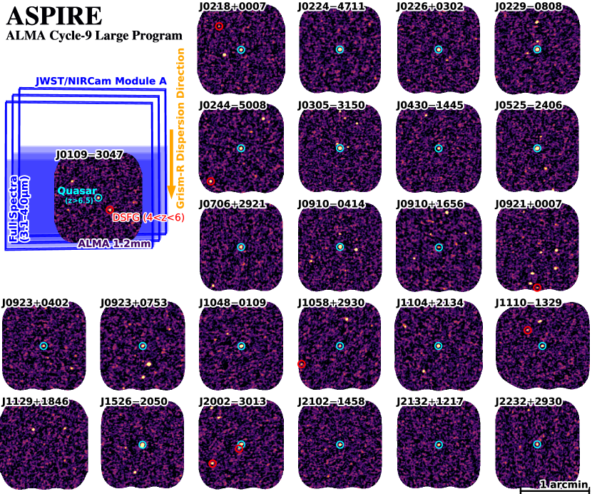
Figure 1: 1.2-mm continuum images of 25 quasar fields obtained by ASPIRE ALMA Cycle-9 large program. In the top-left panel, we highlight the design of JWST/NIRCam and ALMA observations. The whole ALMA 1.2-mm continuum imaging mosaics (uv-tapered with FWHM = 1″) are within the full spectral ($\lambda$ = 3.1–4.0 $\mathrm{\SIUnitSymbolMicro m}$ with F356W filter) coverage region of NIRCam module A as indicated by the blue shaded region. The quasar J0109–3047 ($z=6.791$; cyan circle) is located in the center of ALMA footprint, and one DSFG (J0109m3047.C02 at $z=5.549$) is also highlighted with red circle. The position angle of NIRCam WFSS observation is 270° for J0109 field, and therefore the grism-R dispersion direction is almost from north to south as indicated by the orange arrow. Note that the dispersion direction depends on the JWST/NIRCam PA and varies from field to field. ALMA 1.2-mm continuum images of all the other 24 fields are also displayed. Quasars with continuum detection ($z=6.5-6.8$) and spectroscopically confirmed DSFGs at $z=4-6$ are highlighted in cyan and red circles, respectively. Many DSFGs at other redshifts are also detected with ALMA but not highlighted in this figure.

2.2 ALMA

ALMA 1.2-mm mosaics of all 25 ASPIRE quasar fields were obtained through a 100-hour ALMA Cycle-9 large program (PI: Wang, F.; Program ID: 2022.1.01077.L). In each of the ALMA band-6 mosaics, we tuned the central frequency of the lower sideband as the [C II] line frequency at the quasar redshift (min–median–max: 243.0–247.9–252.9 GHz). Two 1.875–GHz spectral windows were placed to cover the –2200 $\sim$ +2200 $\mathrm{k}\mathrm{m}\,\mathrm{s}^{-1}$ velocity range around the quasar redshift, with the primary goal to blindly detect [C II] emitters at quasar vicinity and measure the Mpc-scale clustering of [C II] emitters around these quasars. Two more spectral windows were placed in the upper sideband to increase the continuum sensitivity, and the final effective frequencies of continuum images are 250.6–255.6–260.6 GHz (min–median–max). As illustrated in Figure 1, in each quasar field, we map the $\sim$ 1$\farcm$2$\times$1$\farcm$1 region centered on the quasar with $\sim$ 23 Nyquist-sampled ALMA 12-m pointings. The ALMA footprints are covered by the full spectral coverage region of NIRCam WFSS at 3.1–4.0 $\mathrm{\SIUnitSymbolMicro m}$, allowing us to search for emission lines from these ALMA sources.

ASPIRE-ALMA observations were conducted from October 14, 2022 to February 14, 2023 through C-2/3 configuration. The typical angular resolution of ALMA observation is $\sim$ 0$\farcs$65. The total survey area of the ASPIRE-ALMA program is 34.9 arcmin² at above a primary beam response limit of 0.25 as adopted in this paper.

We reduced all ALMA data with the standard CASA v6.4.1.12 pipeline (McMullin et al., 2007; CASA Team et al., 2022) for Cycle-9 data. Our data reduction started from raw ALMA science data models with the restoration of pipeline-calibrated, observatory-flagged data through scriptForPI.py. These calibrated measurement sets were then concatenated and imaged based on the North American ALMA imaging script template. To avoid the artificial boost of continuum flux densities from [C II] emitters at quasar redshifts, we first flagged the spectral channels that have a velocity offset smaller than 500 $\mathrm{k}\mathrm{m}\,\mathrm{s}^{-1}$ from the quasar [C II] line center. Noisy spectral channels caused by telluric absorption were also visually identified through command plotms and flagged from continuum imaging. We then split the measurement sets to a channel width of 125 MHz and obtained continuum imaging at both native ALMA resolution (Briggs weighting robust=0.5, no uv–tapering) and tapered resolution (robust=2.0, uv–tapered with Gaussian kernel of FWHM = 1$\farcs$0). The reduction with robust=0.5 weighting is to optimize the sensitivity for compact emission, and our trail suggests that the sensitivity is similar to that of naturally weighted (robust=2.0, no uv–tapering) imaging data products. At tapered resolution, sources with extended structural profile (FWHM $\gtrsim$ 1″) can be detected at higher signal-to-noise ratio (S/N) than that on native-resolution image. The synthesized beam FWHM is $0\farcs 65\pm 0\farcs 05$ and $1\farcs 34\pm 0\farcs 05$ for native and tapered continuum image mosaics, respectively. The image mosaics were produced with tclean command with a pixel size of 0$\farcs$12. We adopted the automatic multi-threshold masking algorithm (Kepley et al., 2020) to save human labor for interactive masking, which is found to be comparably accurate as manual-masking results in our trials. The continuum root-mean-square (RMS) noises (before primary beam response correction) of our ALMA mosaics are 0.031$\pm$0.004 mJy beam^-1 and 0.034$\pm$0.004 mJy beam^-1 at native and tapered resolution, respectively.

ALMA continuum sources were identified on both native and tapered images using the simple find_peaks algorithm in photutils (Bradley et al., 2024). The detailed statistics of ALMA continuum sources at all redshifts will be presented by a forthcoming paper from the collaboration. We select ALMA continuum sources at signal-to-noise ratio $\mathrm{S/N}\geq 5$ in native images or $\mathrm{S/N}\geq 4$ in tapered images (i.e., similar to other ALMA Band-6 continuum surveys, e.g., Fujimoto et al. 2023), resulting in 138 non-repeated peaks. From all ALMA images, we find that the most significant negative peak is at $5.01\sigma$ in native images and $5.04\sigma$ in tapered images, and above our detection threshold there are 1 and 20 negative peaks in the native ($\mathrm{S/N}\leq-5$) and tapered ($\mathrm{S/N}\leq-4$) images, respectively. Therefore, we visually inspected the JWST images of positive peaks that are less significant than the strongest negative peaks, and rejected 20 positive peaks at $\mathrm{S/N}=4-5$ that do not show clear JWST counterpart within 0$\farcs$7. The number of rejected positive peaks is the same as the number of negative peaks above our detection threshold, indicating that spurious continuum sources have been properly removed from our sample.

The final ASPIRE ALMA continuum source sample includes 117 sources (primary beam response $\geq$ 0.25) down to a flux density of $S_{\mathrm{1.2mm}}=0.11$ mJy (median: 0.52 mJy). Among them, 23 sources are targeted quasars at $z=6.5-6.8$, while quasar J0921+0007 ($z=6.5646$; Yang et al. 2021) and the radio-loud quasar J1129+1846 ($z=6.824$; Bañados et al. 2021) are below the ALMA continuum detection limit as shown in Figure 1. After inspecting the JWST images of the remaining 94 sources, we classify all of them as DSFGs at cosmological distances.

3 Analyses

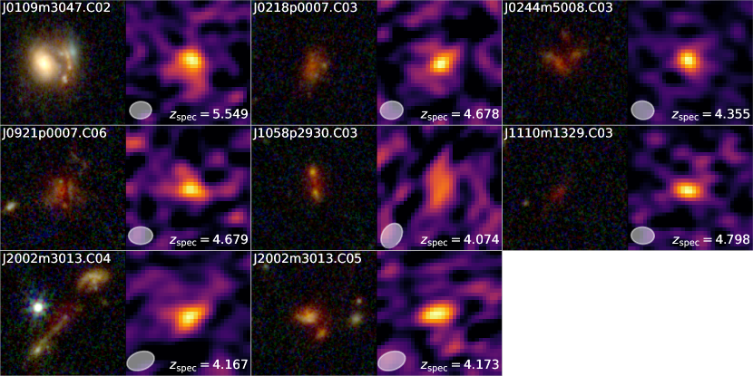
Figure 2: JWST NIRCam (red: F356W; green: F200W, blue: F115W) and ALMA 1.2-mm continuum images of DSFGs at $z=4-6$ discovered with the ASPIRE survey. Image sizes are 4″$\times$4″ (north up, east left). Source ID, spectroscopic redshifts and ALMA beam sizes are indicated in the plots. Most sources appear red in JWST RGB images, indicating that they are highly dust-obscured galaxies at high redshifts. Note that J0109m3047.C02 is gravitationally lensed by the bright galaxy on the left (see Appendix A).

3.1 Spectroscopic Identification of DSFGs at $z=4-6$

To obtain spectroscopic redshifts of the aforementioned 94 ALMA continuum sources (excluding targeted quasars), we extract the NIRCam grism spectra of their JWST counterparts. At 3.1–4.0 $\mathrm{\SIUnitSymbolMicro m}$, we expect to detect emission lines including Paschen $\alpha$ (Pa$\alpha$) at $z=0.7-1.1$, Pa$\beta$ at $z=1.5-2.1$, Pa$\gamma$ and He I $\lambda$10833 at $z=1.9-2.7$, [S III] $\lambda$9533 at $z=2.3-3.1$, [S III] $\lambda$9071 at $z=2.5-3.5$, and most relevantly, H$\alpha$ at $z=3.8-5.0$ and [O III] $\lambda$5008 at $z=5.3-6.9$.

We visually inspect the 2D and 1D grism spectra of all ALMA continuum sources, both before and after continuum subtraction, to identify potential emission lines. Our visual inspection, together with the ALMA [C II] line search (will be presented in a forthcoming paper from the collaboration), yields 16 redshifts at $z=3.8-6.8$ through H$\alpha$, [O III] or [C II] line detections. Six sources are at $z>6$, and all of them are quasar companions ($z=6.5-6.8$). At our interested redshift range $z=4-6$ that is not affected by potential galaxy overdensities associated with quasar, we obtain redshifts for eight sources.

The JWST and ALMA images of these eight sources are displayed in Figure 2. All of these sources are highly secure detections in ALMA (S/N $\geq$ 6.5), and all of them have JWST counterparts detected in the F200W and F356W band. The relative astrometric error between JWST and ALMA images is $\lesssim 0\farcs 1$. Most of these sources appear red (i.e., large F200W–F356W and F115W–F356W color) in the JWST RGB image, indicating that they are highly dust-obscured galaxies at high redshifts. These sources are also clearly resolved at the JWST wavelengths without showing bright point-like structure, indicating that they unlikely host unobscured active galactic nuclei (AGN). Detailed morphological study of ASPIRE DSFGs will be a focus of future work from the collaboration.

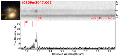
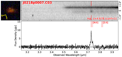
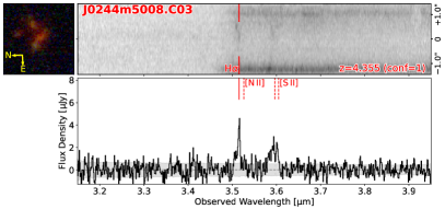
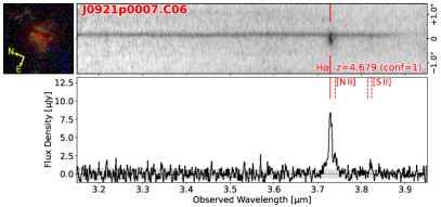
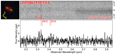
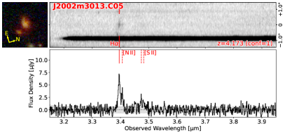
Figure 3: JWST NIRCam image, 2D and 1D spectra of six DSFGs with secure spectroscopic redshifts at $4-6$ (conf=1). Note that the continuum emission (primarily from bright contaminating galaxies) is subtracted in 1D spectra, but not in 2D spectra. NIRCam images are aligned along the dispersion direction (from left to right). Also note that the 2D spectra are compressed in the dispersion direction for display purpose. Primary emission lines (H$\beta$, [O III] $\lambda\lambda$4960,5008, H$\alpha$) are indicated with solid red lines, and other fainter lines ([N II] $\lambda$6585, [S II] $\lambda\lambda$6718,6733) are indicated with dashed red lines.

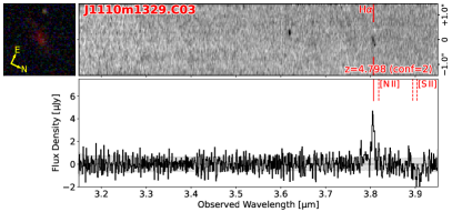
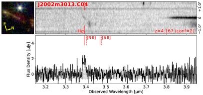
Figure 4: Same as Figure 3 but for two DSFGs with spectroscopic redshifts at $4-6$ based on single emission line (conf=2).

Figure 3 and Figure 4 show the 2D and 1D NIRCam grism spectra of these eight sources, grouped by the confidence level of the redshifts.

We classify the redshifts of six sources as secure (confidence conf=1; Figure 3), as at least two spectral lines are detected (primary line at $\geq 5\sigma$ and secondary line at $\geq 3\sigma$). Among them, the highest-redshift source J0109m3047.C02 is detected in H$\beta$ and [O III] $\lambda\lambda$4960, 5008, confirming the redshift at $z=5.549$. We notice that J0109m3047.C02 is very close to a foreground galaxy ($z_{\mathrm{phot}}=1.18\pm 0.05$, separation $\sim$ 0$\farcs$8). We estimate a gravitational lensing magnification of $\mu=1.91\pm 0.50$ at the centroid of ALMA continuum emission (see details in Appendix A). The other five sources in this group are detected in [N II] $\lambda$6585 and/or [S II] $\lambda\lambda$6718,6733 at $3\sigma$ significance at least, suggesting redshifts at $z=4.07-4.68$.

The remaining two sources in Figure 4 only exhibit single-line detections in NIRCam grism spectra (confidence conf=2). Without the detection of secondary line, it is hard to conclude their nature, but we argue that these emission lines are most likely H$\alpha$ at $z=4.17$ and 4.80. We measure the emission-line flux from the continuum-subtracted 1D spectra through Gaussian-profile fitting, and subtract the line fluxes from the F356W Kron-aperture photometry. We then derive the equivalent widths (EWs) of these lines, finding large observed-frame EWs of 5240$\pm$500 and 890$\pm$270 Å for J1110m1329.C03 and J2002m3013.C04, respectively. Such large EWs are extremely hard to be reproduced with lower-redshift Paschen or He I $\lambda$10833 lines based on the analyses of F444W grism data of DSFGs in the GOODS-S field (FRESCO, Oesch et al. 2023; Boogaard et al. 2024 and Sun, F., private communication), and the most likely line solution is therefore H$\alpha$ or [O III] $\lambda$5008. Therefore, we conclude that:

• J1110m1329.C03: The non-detection of a secondary line indicates that the detected line can only be H$\alpha$ at $z=4.798$, otherwise the [O III] $\lambda$4960 line would have been detected at $>3\sigma$.

• J2002m3013.C04: The wavelength of detected emission line of J2002m3013.C04 is very similar to the H$\alpha$ wavelength of J2002m3013.C05 (velocity offset $\delta v$ = 350 $\mathrm{k}\mathrm{m}\,\mathrm{s}^{-1}$) in the same quasar field, and other line emitter at similar wavelengths are also identified in the vicinity of J2002m3013.C04 (see the 2D spectrum). Therefore, J2002m3013.C04 ($z=4.173$) is likely associated with a group of H$\alpha$ emitters at $z=4.17$.

J1110m1329.C03 and J2002m3013.C04 are the only two single-line emitters in the ASPIRE DSFG sample that are undetected in the F115W band ($<3\sigma$) and thus likely reside at $z>4$, similar to many photometrically selected DSFGs at $z\gtrsim 4$ through JWST imaging surveys (e.g., McKinney et al., 2023a, 2024; Gottumukkala et al., 2024; Williams et al., 2024). For all of the emission line solutions above, we also examine the ALMA spectral cubes to make sure that none of them are mis-identified [O III]$+$[C II] emitters around quasar redshifts. We also experiment other line solutions, e.g., He I $\lambda$10833 and Pa$\gamma$, and we find that these solutions do not match the observed wavelengths or strengths of emission line complexes.

We notice that some of emission lines in Figure 3 and 4 appear to be broad (FWHM $\gtrsim$ 1000 $\mathrm{k}\mathrm{m}\,\mathrm{s}^{-1}$). This is mostly because of morphological broadening with slitless spectroscopy, but not necessarily the presence of AGN. A galaxy with FWHM $\sim$ 0$\farcs$8 will exhibit a line with of $0\farcs 8\cdot(0\farcs 063\,$\mathrm{p}\mathrm{i}\mathrm{x}\mathrm{e}\mathrm{l}^{-1}$)^{-1}(0.98\,$\mathrm{n}\mathrm{m}\,\mathrm{p}\mathrm{i}\mathrm{x}\mathrm{e}\mathrm{l}^{-1}$)\lambda_{\mathrm{obs}}^{-1}c\sim 1000$ $\mathrm{k}\mathrm{m}\,\mathrm{s}^{-1}$ with NIRCam slitless spectroscopy, even without further consideration of instrumental or Doppler broadening. The presence (or not) of broad-line AGN will need to be examined with further slit or integral-field spectroscopy.

Table 1 summarizes the photometric and spectroscopic information of these eight DSFGs at $z=4-6$. We construct the JWST detection image by coadding F200W and F356W images, create image segments for regions that have at least 10 continuous pixels detected at $\geq 5\sigma$, and then obtain aperture photometry using the Kron parameters k=2.5 and Rmin=1.2 in all JWST bands. The photometry of J0109m3047.C02 is obtained on the residual images with other foreground galaxies modeled and subtracted with galfit (Peng et al. 2010; Appendix A). The photometric uncertainty is estimated from sky background with a conservative noise floor of 5% following the practice of NIRCam guaranteed-time-observation team (e.g., Tacchella et al. 2023).

At the ALMA wavelength, we adopt the peak flux densities of sources in the uv-tapered images ($f_{\mathrm{tap}}$) multiplied by a factor of 1.1. This is because we find that the scaled-up $f_{\mathrm{tap}}$ is systematically consistent with the flux densities measured with $r=1\arcsec$ aperture ($f_{\mathrm{aper}}$) and casa image-plane fitting (imfit; $f_{\mathrm{imfit}}$) in the native-resolution images, but with considerably smaller uncertainties. The scaling factor is also verified with the injection experiment detailed in Appendix B.

For H$\alpha$ emitters, we measure the emission-line fluxes through multi-component Gaussian-profile fitting. For J0109m3047.C02 with complex morphological and thus line profile, we integrate the 1D spectrum within 20 Å (rest-frame) from the line center to derive the line fluxes.

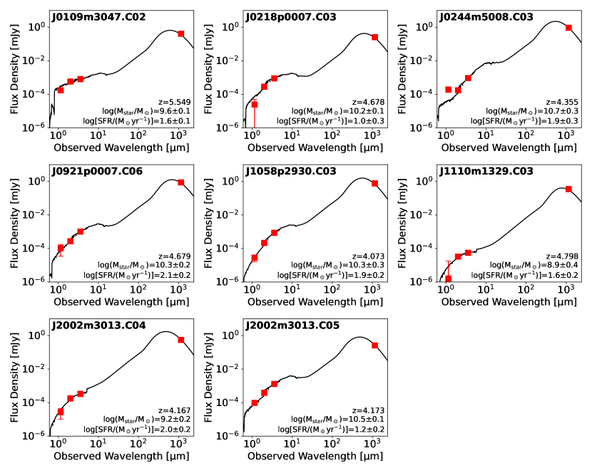
Figure 5: JWST and ALMA SEDs of eight DSFGs in ASPIRE sample. Photometric measurements are shown as red squares. Best-fit SED models obtained with CIGALE are shown as solid black curves. Source ID, redshifts and derived stellar masses, SFRs are indicated in the plots.

Table 1: Photometric and spectroscopic properties of ASPIRE DSFGs at $z=4-6$

ID	R.A.	Decl.	$\mathrm{S/N}$	PB	$S_{\mathrm{1.2mm}}$	$z_{\mathrm{spec}}$	conf	F115W	F200W	F356W	$f_{\mathrm{line}}$
	[deg]	[deg]			[mJy]			[mag]	[mag]	[mag]	[$\mathrm{1}\mathrm{0}^{-18}\,\mathrm{e}\mathrm{r}\mathrm{g}\,\mathrm{s}^{-1}\,\mathrm{c}\mathrm{m}^{-2}$]
J0109m3047.C02	$17.46807$	$-30.79361$	12.5	1.00	0.45$\pm$0.04	5.549	1	26.01$\pm$0.19	24.73$\pm$0.05	23.94$\pm$0.05	53.7$\pm$1.2
J0218p0007.C03	$34.70137$	$0.12652$	6.5	0.88	0.28$\pm$0.04	4.678	1	$>26.70$	25.26$\pm$0.05	23.89$\pm$0.05	15.8$\pm$0.7
J0244m5008.C03	$41.01580$	$-50.15628$	13.4	0.51	1.03$\pm$0.08	4.355	1	25.69$\pm$0.35	25.80$\pm$0.07	23.94$\pm$0.05	5.9$\pm$0.5
J0921p0007.C06	$140.33569$	$0.11316$	6.7	0.31	0.96$\pm$0.14	4.679	1	$>25.60$	25.32$\pm$0.07	23.76$\pm$0.05	15.8$\pm$0.7
J1058p2930.C03	$164.54289$	$29.50715$	6.6	0.31	0.84$\pm$0.13	4.074	1	$>27.49$	25.58$\pm$0.05	24.03$\pm$0.05	3.6$\pm$0.7
J1110m1329.C03	$167.64528$	$-13.49222$	9.1	0.99	0.38$\pm$0.04	4.798	2	$>27.20$	27.62$\pm$0.22	26.42$\pm$0.05	6.0$\pm$0.6
J2002m3013.C04	$300.68137$	$-30.22729$	11.2	0.76	0.61$\pm$0.05	4.167	2	$>27.14$	25.77$\pm$0.07	24.99$\pm$0.05	7.6$\pm$2.3
J2002m3013.C05	$300.67392$	$-30.22369$	7.0	1.00	0.29$\pm$0.04	4.173	1	26.44$\pm$0.14	24.94$\pm$0.05	23.54$\pm$0.05	13.2$\pm$0.9

Note. — S/N is the maximum S/N measured from ALMA native-resolution and uv-tapered map. PB is the ALMA primary beam response. $S_{\mathrm{1.2mm}}$ is the ALMA continuum flux density measured from the peak of uv-tapered map, corrected for primary beam response and multiplied by a factor of 1.1 to match the flux densities measured from aperture and CASA image-plane fitting (imfit; Section 3.1). The uncertainty for spectroscopic redshift is $\Delta z\sim 0.002$, mostly propagated from the wavelength calibration error of NIRCam WFSS. $f_{\mathrm{line}}$ is the [O III] $\lambda$5008 (for J0109m3047.C02) or H$\alpha$ (for other sources) line fluxes measured from 1D NIRCam grism spectra. Lensing magnification is not corrected for J0109m3047.C02 (see Appendix A).

Table 2: Physical properties of ASPIRE DSFGs at $z=4-6$ derived from SED modeling

ID	$\log[M_{\mathrm{star}}/\mathrm{M}_{\odot}]$	$\log[\mathrm{SFR}_{\mathrm{10Myrs}}/(\mathrm{M}_{\odot}\,\mathrm{yr}^{-1})]$	$\log[\mathrm{SFR}_{\mathrm{UV}}/(\mathrm{M}_{\odot}\,\mathrm{yr}^{-1})]$	$\log[L_{\mathrm{IR}}/\mathrm{L}_{\odot}]$	$A_{V}$/mag
J0109m3047.C02	9.6$\pm$0.1	1.6$\pm$0.1	$0.9\pm$0.1	11.5$\pm$0.1	0.6$\pm$0.1
J0218p0007.C03	10.2$\pm$0.1	1.0$\pm$0.3	$<0.4$	11.4$\pm$0.1	0.9$\pm$0.2
J0244m5008.C03	10.7$\pm$0.3	1.9$\pm$0.3	$0.8\pm$0.1	12.1$\pm$0.2	2.4$\pm$0.4
J0921p0007.C06	10.3$\pm$0.2	2.1$\pm$0.2	$<0.9$	12.0$\pm$0.1	1.5$\pm$0.3
J1058p2930.C03	10.3$\pm$0.3	1.9$\pm$0.2	$-0.1\pm$0.2	11.9$\pm$0.1	2.0$\pm$0.3
J1110m1329.C03	8.9$\pm$0.4	1.6$\pm$0.2	$<0.2$	11.4$\pm$0.2	2.1$\pm$0.5
J2002m3013.C04	9.2$\pm$0.2	2.0$\pm$0.2	$<0.2$	11.8$\pm$0.2	1.5$\pm$0.2
J2002m3013.C05	10.5$\pm$0.1	1.2$\pm$0.2	$0.4\pm$0.1	11.6$\pm$0.1	1.4$\pm$0.3

Note. — Light-weighted differential lensing magnification has been corrected for J0109m3047.C02 (see details in Appendix A). $\mathrm{SFR}_{\mathrm{10Myrs}}$ is the SFR averaged over the last 10 Myrs of SFH, which is slightly different from the dust-obscured $\mathrm{SFR}_{\mathrm{IR}}$ (based on $L_{\mathrm{IR}}$) that we use to infer the obscured SFRD (Section 4.4).

3.2 SED Modeling

We obtain physical SED modeling of eight ASPIRE DSFGs at $z=4-6$ using software CIGALE (Noll et al., 2009; Boquien et al., 2019). We use four-band NIRCam and ALMA photometry for the fitting. Because the rest-frame far-IR SEDs are only loosely constrained by ALMA photometry in one band, we have to rely on the energy balance assumption with CIGALE to infer the IR luminosity and thus obscured SFR. In Section 5.1, we discuss the validity of energy balance assumption and impact from uncertain dust temperature.

We assume a commonly used delayed-$\tau$ star-formation history (SFH), in which $\mathrm{SFR}(t)\propto t\exp(-t/\tau)$ and $\tau$ is the peak time of star formation. We allow the age of main stellar population to be 10–500 Myr and $\tau$ to be 30–3000 Myr. An optional late starburst is allowed in the last 10 Myr of SFH, which could produce up to 20% of total stellar mass. We use Bruzual & Charlot (2003) stellar population synthesis models, and allow a metallicity range of 0.4$Z_{\odot}$–$Z_{\odot}$. We adopt a modified Calzetti et al. 2000 attenuation curve, and allow the variation of the power-law slope by $\pm$0.3 and $A_{V}$ effectively at 0–10. For simplicity, we assume Casey (2012) mid-to-far-IR dust continuum model that could be parameterized by dust temperature ($T_{\mathrm{dust}}$; flat prior at 30–50 K), dust emissivity ($\beta_{\mathrm{em}}$, fixed at 1.8) and mid-IR power-law slope ($\alpha_{\mathrm{MIR}}$, fixed at 2.0). Although the Casey (2012) model does not include mid-IR polycyclic aromatic hydrocarbon (PAH) features, the inclusion of mid-IR power-law slope can well reproduce the luminosity excess from PAHs from a comparison of widely used empirical SED templates (e.g., Chary & Elbaz, 2001; Rieke et al., 2009, uncertainty $\lesssim$0.1 dex). Note that we do not include nebular emission in the SED modeling for simplicity. Instead, we subtract the identified emission line fluxes (H$\alpha$, [O III], H$\beta$, [N II] and [S II]) from the F356W photometry, and perform the SED fitting for pure stellar and dust continuum. For J0109m3047.C02, we correct for the differential lensing magnification in the SED modeling (Appendix A).

Figure 5 shows the best-fit SED models of eight DSFGs in our sample, and the derived physical parameters are presented in Table 2. We observe a median stellar mass $\log(M_{\mathrm{star}}/$\mathrm{M}_{\odot}$)=10.3\pm 0.2$ for sources in our sample, and the median IR luminosity is $\log(L_{\mathrm{IR}}/$\mathrm{L}_{\odot}$)=11.7\pm 0.1$, i.e., comparable to LIRGs in the local Universe. We also derive UV SFR for each source through the observed F115W flux density (rest-frame $\sim$2000 Å) and the conversion $\mathrm{SFR}_{\mathrm{UV}}/($\mathrm{M}_{\odot}\,\mathrm{y}\mathrm{r}^{-1}$)=8.8\times 10^{-29}\,L_{\mathrm{FUV}}/($\mathrm{e}\mathrm{r}\mathrm{g}\,\mathrm{s}^{-1}\,\mathrm{H}\mathrm{z}^{-1}$)$ (Madau & Dickinson 2014 but assuming Chabrier 2003 IMF). Under the same IMF assumption, the conversion between IR luminosity and dust-obscured SFR is $\mathrm{SFR}_{\mathrm{IR}}/($\mathrm{M}_{\odot}\,\mathrm{y}\mathrm{r}^{-1}$)=1.1\times 10^{-10}\,L_{\mathrm{IR}}/$\mathrm{L}_{\odot}$$, and the conversion between H$\alpha$ luminosity and SFR is $\mathrm{SFR}_{\mathrm{H\alpha}}/($\mathrm{M}_{\odot}\,\mathrm{y}\mathrm{r}^{-1}$)=5\times 10^{-42}\,L_{\mathrm{H\alpha}}/($\mathrm{e}\mathrm{r}\mathrm{g}\,\mathrm{s}^{-1}\mathrm{)}$$ (Kennicutt, 1998).

4 Results

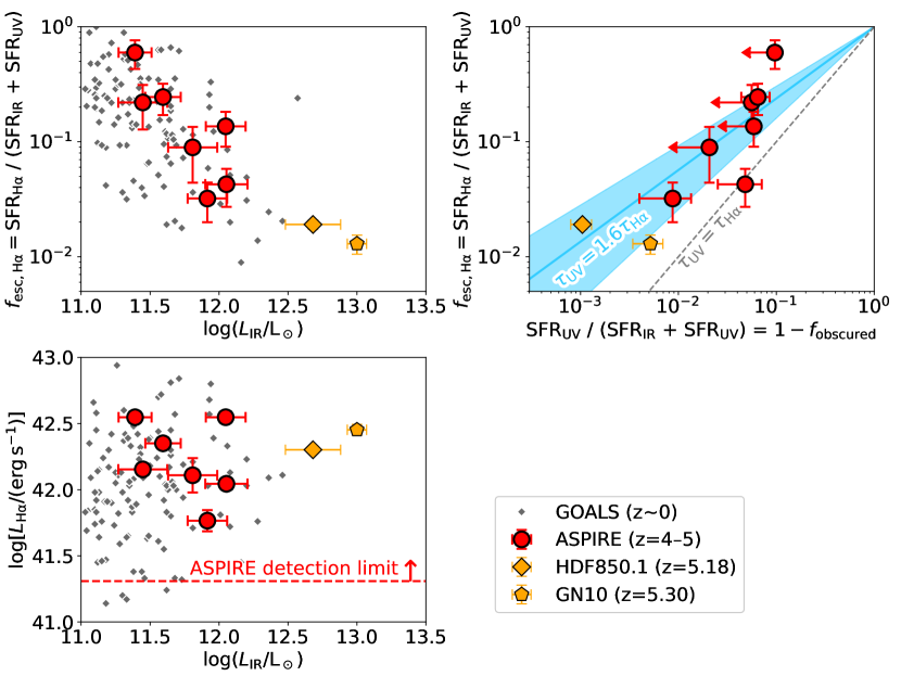
Figure 6: The dust obscuration and escape of H$\alpha$ photons from DSFGs. In the top-left panel, we show the escape fraction of H$\alpha$ photons versus IR luminosity. ASPIRE DSFGs are shown in red circles and two $z>5$ DSFGs in the FRESCO GOODS-N field (HDF850.1, GN10; measurements from Sun et al. 2024) are shown in orange symbols. Local (U)LIRGs in the GOALS sample are shown as small gray diamonds (Armus et al., 2009; Jin et al., 2019a). DSFGs with higher $L_{\mathrm{IR}}$ exhibit smaller escape fraction of H$\alpha$ photons, resulting in a nearly constant H$\alpha$ luminosity, i.e., $\log[L_{\mathrm{H\alpha}}/($\mathrm{e}\mathrm{r}\mathrm{g}\,\mathrm{s}^{-1}$)]\simeq 42.0-42.5$, across a $\sim$ 2-dex wide span of $L_{\mathrm{IR}}$ as shown in the bottom-left panel. In the top-right panel, we plot the escape fraction of H$\alpha$ versus the escape fraction of UV ($1-f_{\mathrm{obscured}}$). The dashed gray line indicates the scenario that the optical depths at UV ($\tau_{\mathrm{UV}}$; $\sim$ 2000 Å) and H$\alpha$ ($\tau_{\mathrm{H\alpha}}$) wavelength are identical. The solid blue line and shaded region indicate the best-fit scaling relation and uncertainty $\tau_{\mathrm{UV}}=(1.61\pm 0.34)\,\tau_{\mathrm{H\alpha}}$.

4.1 Obscured Fraction of UV and H$\alpha$ Star Formation

Most star formation in our ASPIRE DSFG sample at $z=4-6$ is obscured by dust. If we define the obscured fraction of SFR as $f_{\mathrm{obscured}}=\mathrm{SFR}_{\mathrm{IR}}/(\mathrm{SFR}_{\mathrm{IR}}+\mathrm{SFR}_{\mathrm{UV}})$ (e.g., Whitaker et al., 2017; Fudamoto et al., 2020), then 96$\pm$2% of their star formation is obscured by dust. Such an obscured fraction of SFR is significantly higher than the ALPINE sample of $M_{\mathrm{star}}$-selected galaxies with comparable mass and redshifts ($f_{\mathrm{obscured}}=67_{-7}^{+5}\%$; Fudamoto et al. 2020), suggesting that these ASPIRE DSFGs represent the dusty tail of the distribution of a wider star-forming galaxy population at this epoch. The obscured fractions of SFR for ASPIRE DSFGs are still slightly less than that of the most extreme DSFG at $z\sim 5$, e.g., HDF850.1 at $z=5.18$ (Hughes et al., 1998; Walter et al., 2012), whose obscured fraction is $f_{\mathrm{obscured}}\sim 99.9\%$ (Sun et al. 2024; see also Herard-Demanche et al. 2023, Xiao et al. 2023a). We also notice that Zimmerman et al. (2024) suggests an increase of $f_{\mathrm{obscured}}$ at fixed stellar mass at higher redshifts in the simba cosmological simulations.

Among the ASPIRE DSFG sample at $z=4-6$, five galaxies are undetected in the F115W band (rest-frame $\sim$ 2000 Å) and therefore they could be classified as HST-dark galaxies as introduced in Section 1. However, this is only a subset of 14 HST-dark galaxies selected with ALMA continuum detection and F115W non-detection ($<3\sigma$) among the full ASPIRE DSFG sample across all redshifts. This suggests a complex and broad redshift distribution of HST-dark galaxies, and the photometric redshifts obtained in optical and near-IR can be strongly degenerate with the dust attenuation and stellar age of the galaxies (e.g., Huang et al., 2011; Caputi et al., 2012; Wang et al., 2016). Fortunately, the successful detections of H$\alpha$ and [O III] lines of these highly obscured DSFGs through NIRCam WFSS provide the critical redshift confirmation, allowing us to study the dust attenuation in these DSFGs with much higher accuracy than sources without $z_{\mathrm{spec}}$.

The top-left panel of Figure 6 shows the escape fraction of H$\alpha$ photons (defined as $f_{\mathrm{esc,H\alpha}}=\mathrm{SFR}_{\mathrm{H\alpha}}/(\mathrm{SFR}_{\mathrm{UV}}+\mathrm{SFR}_{\mathrm{IR}})$; not to confuse with the escape fraction in reionization/IGM context) versus $L_{\mathrm{IR}}$. Assuming a constant SFH, $f_{\mathrm{esc,H\alpha}}$ is mainly controlled by the dust extinction (although caution that compared to IR luminosity, H$\alpha$ luminosity is less sensitive to star formation at $\gtrsim$10 Myr; see recent study of a $z=2.4$ post-starburst DSFGs by Cooper et al. 2024). It is clear that $f_{\mathrm{esc,H\alpha}}$ is strongly anti-correlated with $L_{\mathrm{IR}}$, both at $z\sim 5$ or in the local Universe (as seen with the LIRGs/ULIRGs in the GOALS sample; Armus et al. 2009, Jin et al. 2019a). Such an anti-correlation indicates that a larger fraction of H$\alpha$ photons is dust-obscured in DSFG with more vigorous star formation activity. This is mainly driven by the fact that H$\alpha$ luminosity of $z\sim 5$ DSFG does not correlate with $L_{\mathrm{IR}}$ (Spearman’s $\rho=-0.05$, $p$-value = 0.9) because of complex dust-stellar geometry (e.g., García-Marín et al., 2009; Giménez-Arteaga et al., 2022). As shown in the bottom-left panel of Figure 6, the H$\alpha$ luminosity of $z\sim 5$ DSFG remains almost constant (i.e., $\log[L_{\mathrm{H\alpha}}/($\mathrm{e}\mathrm{r}\mathrm{g}\,\mathrm{s}^{-1}$)]\simeq 42.0-42.5$) across an almost  2-dex wide span of $L_{\mathrm{IR}}$. Such a characteristic H$\alpha$ luminosity range is well above the $5\sigma$ detection limit of ASPIRE (and also FRESCO; Oesch et al. 2023). Also as shown in the same plot, if local (U)LIRGs are placed at $z\sim 5$, 96% of them would be above our ASPIRE H$\alpha$ luminosity detection threshold. Therefore, we conclude that the NIRCam grism spectroscopic surveys of high-redshift DSFGs are highly efficient and complete.

The escape fraction of UV photons (defined as $f_{\mathrm{esc,UV}}=1-f_{\mathrm{obscured}}=\mathrm{SFR}_{\mathrm{UV}}/(\mathrm{SFR}_{\mathrm{IR}}+\mathrm{SFR}_{\mathrm{UV}})$) is also controlled by dust extinction under the stable SFH assumption. A tight correlation between $f_{\mathrm{esc,UV}}$ and $f_{\mathrm{esc,H\alpha}}$ can demonstrate that these escape fractions are mostly driven by the dust obscuration instead of complex SFH because UV, H$\alpha$ and far-IR emission is sensitive to SFH at different timescales. Therefore, we compare the escape fraction of H$\alpha$ and UV photons in the top-right panel of Figure 6. Both UV and H$\alpha$ escape fractions are controlled by the optical depth at their wavelengths, i.e., $f_{\mathrm{esc,UV}}=\exp(-\tau_{\mathrm{UV}})$ and $f_{\mathrm{esc,H\alpha}}=\exp(-\tau_{\mathrm{H\alpha}})$. We find that the typical $\tau_{\mathrm{UV}}/\tau_{\mathrm{H\alpha}}$ ratio of $z\sim 5$ DSFGs is $1.61\pm 0.34$.

Under Calzetti et al. (2000) extinction curve with negligible 2175-Å bump, the dust optical depth ratio between UV ($\sim$ 2000 Å) and H$\alpha$ wavelength is $\sim$ 2.7. This is larger than the ratio derived above because nebular emission lines originate from stellar birth clouds with stronger dust attenuation, and in certain cases H$\alpha$ from IR-luminous regions could be totally obscured (e.g., Pereira-Santaella et al., 2015; Colina et al., 2023; Bik et al., 2024; Sun et al., 2024; Übler et al., 2024). Therefore, the reduction factor to be applied on the nebular gas emission line $E(B-V)_{g}$ to derive stellar continuum $E(B-V)_{s}$ is $0.60\pm 0.13$ for $z\sim 5$ DSFGs, which is slightly higher than the canonical factor of 0.44$\pm$0.03 with Calzetti et al. (2000) extinction curve (Calzetti, 1997). A larger reduction factor suggests that the difference of dust geometry between UV and nebular emission is smaller for $z\sim 5$ DSFGs when compared to local starburst galaxies. This also increases the detectability of H$\alpha$ emission of DSFGs at high redshifts. However, we also notice that the reduction factor is sensitive to the slope of underlying extinction curve. If the underlying extinction curve of high-redshift DSFGs is steeper, i.e., following the SMC curve (Gordon et al., 2003), then the reduction factor could be smaller (0.38$\pm$0.08).

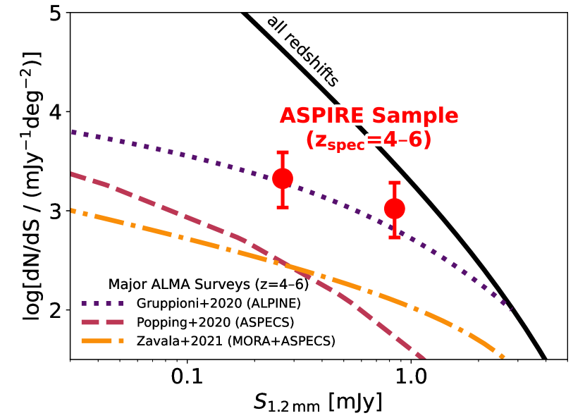
Figure 7: Differential 1.2-mm number count of DSFGs at $z=4-6$ measured with the ASPIRE sample (solid red circles). For comparison we show the 1.2-mm number count of DSFGs at all redshifts (Fujimoto et al. 2023; solid black line), and the number count of DSFGs at $z=4-6$ estimated based on Gruppioni et al. (2020, based on ALPINE survey; dotted purple line) and Zavala et al. (2021, based on MORA and ASPECS survey; dashed-dotted orange line) assuming their best-fit IRLFs and galaxy SEDs, and the semi–empirical model from Popping et al. (2020, based on ASPECS survey; dashed maroon line).

4.2 Number Count of DSFGs at $z=4-6$

One key focus of this study is to understand the number density of DSFGs at $z=4-6$ and their contribution to the IRLF and SFRD. To measure these quantities, we first compute the effective survey area at above our detection limits in the native and tapered ALMA mosaics. We make use of the RMS noises of these mosaics and the primary beam response maps to compute the effective survey area above each flux density limits, i.e., $A_{\mathrm{max}}(S_{\mathrm{1.2\,mm}})$. Given the brightness of galaxies in our sample (observed $S_{\mathrm{1.2mm}}\geq 0.28$ mJy; much larger than the $\sim$ 0.15 mJy detection limit), these sources can be selected in most of our survey footprint ($A_{\mathrm{max}}$ ranges from 24 to 35 arcmin² for each source). Note that for the lensed source J0109m3047.C02, the $A_{\mathrm{max}}$ is computed using the lensing-corrected 1.2-mm flux density ($S_{\mathrm{1.2mm}}=0.24$ mJy).

By simply summing the $1/A_{\mathrm{max}}$ of ASPIRE DSFGs and correcting for the redshift desert at $z\simeq 5.0-5.3$ where H$\alpha$ or [O III] cannot be detected with NIRCam WFSS survey with the F356W filter, we find a surface density of $\sim 1.1\times 10^{3}$ $\mathrm{d}\mathrm{e}\mathrm{g}^{-2}$ for $z=4-6$ DSFGs at $S_{\mathrm{1.2\,mm}}\geq 0.24$ mJy. This is roughly twice of surface density of the HST $H$-dropout galaxies at $z\simeq 3-6$ and $S_{\mathrm{0.87\,mm}}\geq 0.6$ mJy ($\sim$ 530 $\mathrm{d}\mathrm{e}\mathrm{g}^{-2}$; Wang et al. 2019b). The survey depth in terms of $L_{\mathrm{IR}}$ is very similar for ASPIRE and the ALMA follow-up studies in Wang et al. (2019b). Although the conventional $H$-dropout selection with HST and Spitzer/IRAC has identified obscured star formation that was previously missed by rest-frame UV surveys, such a selection will also miss (i) $z>4$ DSFGs that are not totally obscured at HST wavelengths ($J$–$H$ band), e.g., because of patchy dust geometry, and (ii) highly dust-attenuated objects that are faint at 3–5 $\mathrm{\SIUnitSymbolMicro m}$ and below the Spitzer/IRAC detection limit.

We measure the differential number count ($dN/dS$) of ASPIRE DSFGs at $z=4-6$ through the $1/A_{\mathrm{max}}$ method:

$$\frac{dN}{dS}=\frac{1}{d\log S}\sum_{i}\frac{1}{C_{i}A_{\mathrm{max}}(S_{i})}$$ (1)

where $d\log S$ is the flux density bin size in log scale, $C_{i}$ is the completeness for the $i$-th source in the bin, and $A_{\mathrm{max}}(S_{i})$ is the effective survey area at above the source flux density $S_{i}$.

We present the completeness correction simulation in Appendix B, and as a quick summary, our ALMA continuum source selection is highly complete ($>$ 95% for all sources) because of high fidelity of detections ($\mathrm{S/N}\geq 6.5$). Strictly speaking, because of multiple redshift gaps with NIRCam WFSS survey in the F356W band (Section 3.1), the full ASPIRE DSFG sample is not spectroscopically complete across all redshifts. However, we argue that we have reached a high spectroscopic completeness at $z=4-5$ and 5.3–6 because the H$\alpha$ and [O III] luminosity of sources in our sample are well above the $5\sigma$ detection limit (indicated by the dashed red line in low-left panel of Figure 6). Even if the completeness of [O III] spectroscopy for DSFGs cannot be properly assessed because of limited JWST data taken so far (high-redshift DSFGs may exhibit a diverse distribution of [O III] strengths; e.g., McKinney et al. 2023b; Barrufet et al. 2024; Sun et al. 2024), we argue that the number density of DSFGs at $z>5$ should be naturally smaller than that at $z<5$, same as we observed. Therefore, the true number density of DSFGs at $z=4-6$ should be close to our measurement, or just slightly higher.

We set two flux density bins at 0.15–0.47 and 0.47–1.5 mJy (bin size is 0.5 dex). We also run Monte Carlo (MC) simulation to draw 1.2-mm flux density from the observed values and errors, compute the corresponding $A_{\mathrm{max}}$ and completeness and then derive the number count and its uncertainty. The uncertainty includes Poisson error following the prescription of Gehrels (1986), and we also include the error from cosmic variance (shot noise) following the prescription of Moster et al. (2011, same as the method adopted by for DSFGs in the COSMOS-web field), which is computed using the geometry of survey footprint (25 fields with area of 1$\farcm$2$\times$1$\farcm$2), redshift interval ($\Delta z=1.7$ around $z=5$), dark matter correlation function, $\sigma_{8}$ and galaxy bias at $z\sim 5$ (0.17 and and $\sim$8). The uncertainty from cosmic variance ($\sim$0.05 dex) is much smaller than that from Poisson error ($\sim$0.28 dex in each bin), and we also experiment other cosmic variance prescriptions and find similar results (0.05–0.07 dex; Trenti & Stiavelli, 2008; Driver & Robotham, 2010).

Figure 7 shows the 1.2-mm number of DSFGs at $z=4-6$ measured from the ASPIRE survey (red circles). We highlight the fact that the only noticeable uncertainty of our measurement is from Poisson statistics, nor cosmic variance or any other astrophysical assumption (e.g., $z_{\mathrm{phot}}$ or SED model). The number count of $z=4-6$ DSFGs seems to be much flatter than the 1.2-mm number count of DSFGs across all redshifts (solid black line, Fujimoto et al. 2023; see also Fujimoto et al. 2016; González-López et al. 2020; Gómez-Guijarro et al. 2022; Chen et al. 2023; Adscheid et al. 2024 that cover similar $S_{\mathrm{1.2mm}}$ space). This indicates a larger fraction of DSFGs at higher redshifts toward the bright end of millimeter number count function (e.g., Béthermin et al., 2017; Casey et al., 2018b, 2021; Lagos et al., 2020; Sun et al., 2022; Chen et al., 2022).

For comparison, we also show the number count of DSFGs at $z=4-6$ based on the semi-empirical model from Popping et al. (2020, based on ASPECS survey) and IRLFs modeled by Gruppioni et al. (2020, based on ALPINE survey) and Zavala et al. (2021, based on MORA and ASPECS survey). To convert IRLFs in literature to number counts, we assume similar far-IR SEDs as those assumed in these original works. In Zavala et al. (2021), the authors derived a best-fit dust emissivity $\beta_{\mathrm{em}}\sim 1.8$ from their backward modeling, and they assumed a relation between the rest-frame wavelength of far-IR SED peak and IR luminosity ($\lambda_{\mathrm{peak}}-L_{\mathrm{IR}}$; Casey et al. 2018b), which corresponds to a modified blackbody (MBB) $T_{\mathrm{dust}}\sim 32$ K at $L_{\mathrm{IR}}=10^{12}$ $\mathrm{L}_{\odot}$ through Casey 2012 parametrization. In Gruppioni et al. (2020), the authors made use of best-fit far-IR SED through multiple templates included in the software Le Phare (Arnouts & Ilbert, 2011). Therefore, we convert their best-fit IRLF at $z=3.5-6$ to 1.2-mm number count assuming the Chary & Elbaz (2001) far-IR SED templates, one of the major template sets adopted by Le Phare (effectively $T_{\mathrm{dust}}\sim 45$ K and $\beta_{\mathrm{em}}\sim 1.5$ for $S_{\mathrm{1.2mm}}\sim 0.5$ mJy sources at $z\sim 5$).

The number count of $z=4-6$ DSFGs from ASPIRE sample is similar to that of Gruppioni et al. (2020) based on non-target ALMA Band-7 continuum galaxies discovered through ALPINE survey (Béthermin et al., 2020; Le Fèvre et al., 2020). Because the primary targets of ALPINE survey are star-forming galaxies at $z\sim 5$, it has been speculated that the excess of $z=4-6$ DSFG number count from ALPINE (relative to ASPECS) may arise from the clustering of non-target DSFGs around their main targets (e.g., Zavala et al., 2021). Our observations suggest that the number density of $z=4-6$ DSFG measured from ALPINE survey is sufficiently accurate despite uncertainties with $z_{\mathrm{phot}}$.

Our measurements are higher than the models based on ASPECS survey (Popping et al., 2020; Zavala et al., 2021) by $\sim$ 1 dex. Such a large discrepancy cannot be explained by any form of error from the ASPIRE sample. We think the large difference is caused by the strong shot noise with the ASPECS sample ($\sigma\sim 0.5$ dex, including both Poisson error and cosmic variance). Aravena et al. (2020) showed that no DSFG at $z>4$ was blindly discovered with the ASPECS deep 1-mm or 3-mm survey. In contrast, the eight DSFGs in our sample are discovered along 7 out of 25 quasar sightlines, and therefore the chance to detect one DSFG at $z=4-6$ within the 1.4-arcmin² survey area per sightline is only 28%. The survey area of ASPECS in the HUDF is $\sim$ 3 times of a typical ASPIRE field/sightline, and thus the chance to detect zero DSFG at $z=4-6$ is $(1-28\%)^{3}\sim 37$%, a non-negligible probability. Therefore, we attribute the discrepancy between ASPIRE and ASPECS measurements to the underdensity of $z=4-6$ DSFG in the HUDF region. Similar conclusions have been drawn from previous studies for DSFGs (e.g., Fujimoto et al., 2023) and even for Lyman-break galaxies and AGN (e.g., Cowie et al., 2002; Moretti et al., 2003; Bauer et al., 2004; Oesch et al., 2007).

Figure 8: Spectroscopically complete infrared luminosity function at $z=4-6$ measured with the ASPIRE sample (solid red circles). The best-fit IRLF and its uncertainties (16–84th percentile) are indicated with the solid red line and shaded region, respectively. For comparison we show the direct measurements from previous observations (incomplete with spectroscopy) as open gray symbols, which include Koprowski et al. (2017), Wang et al. (2019a), Gruppioni et al. (2020), Fujimoto et al. (2023), Traina et al. (2024). Theoretical model predictions are shown as colored lines including EAGLE (Trayford et al., 2020), FLARES (Vijayan et al., 2022), SIDES (Béthermin et al., 2022) and SHARK (Lagos et al., 2020).

Table 3: Infrared luminosity function at $z=4-6$ measured with ASPIRE DSFGs

Observed infrared luminosity function
$\log(L_{\mathrm{IR}}/$\mathrm{L}_{\odot}$)$	11.2–11.6	11.6–12.0	12.0–12.4
$<N>$	2.71	2.88	1.63
$\log[\Phi/(\mathrm{Mpc}^{-3}\mathrm{dex}^{-1})]$	$-4.04_{-0.39}^{+0.35}$	$-4.27_{-0.39}^{+0.35}$	$-4.51_{-0.50}^{+0.42}$
Best-fit double-power-law parameters
$\log[\Phi^{\star}/(\mathrm{Mpc}^{-3}\mathrm{dex}^{-1})]$	$\log(L_{\mathrm{IR}}^{\star}/L_{\odot})$	$\alpha$	$\beta$
$-4.52_{-0.55}^{+0.49}$	$12.58_{-0.29}^{+0.26}$	$0.59_{-0.45}^{+0.39}$	$3.24_{-0.95}^{+1.63}$

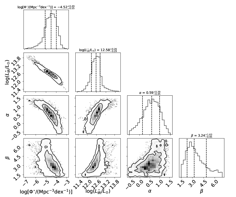
Figure 9: MCMC corner plot of the double-power-law parameters for the IRLF fitting (Figure 8 and Section 4.3). Contours are at $1-2\sigma$.

4.3 Spectroscopically Complete Infrared Luminosity Function

We further measure the IRLF at $z=4-6$ from the ASPIRE DSFG sample. Such an IRLF is spectroscopically complete down to $L_{\mathrm{IR}}\sim 2\times 10^{11}$ $\mathrm{L}_{\odot}$ and almost free from the impact of cosmic variance. Similar to the method present in Section 4.2, we adopt the $1/V_{\mathrm{max}}$ method (Schmidt, 1968):

$$\Phi(L)=\frac{1}{d\log L}\sum_{i}\frac{1}{C_{i}V_{\mathrm{max}}(L_{i})}$$ (2)

where $d\log L$ is the luminosity bin size in log scale, $C_{i}$ is the completeness for the $i$-th source in the bin, and $V_{\mathrm{max}}(L_{i})$ is the effective survey volume at above the source luminosity $L_{i}$. We make use of $L_{\mathrm{IR}}$ and uncertainties measured from CIGALE energy-balance SED fitting. The uncertainty of $L_{\mathrm{IR}}$ and IRLF propagated from loosely constrained $T_{\mathrm{dust}}$ is further discussed in Section 5.1.

We set three $L_{\mathrm{IR}}$ bins at $10^{11.2}-10^{11.6}$, $10^{11.6}-10^{12.0}$ and $10^{12.0}-10^{12.4}$ $\mathrm{L}_{\odot}$. Similarly to Section 4.2, we also run MC simulation to randomly draw $L_{\mathrm{IR}}$ from the SED-derived $L_{\mathrm{IR}}$ and uncertainties. The ratio of drawn $L_{\mathrm{IR}}$ and best-fit $L_{\mathrm{IR}}$ is applied to scale the ALMA S/N for the completeness and effective survey volume calculation. The uncertainty of our luminosity function measurements include the standard deviation from MC simulation, Poisson error (following Gehrels 1986) and cosmic variance ($\sim$ 0.03 dex, negligible; following Moster et al. 2011 prescription), respectively. The derived IRLF is presented in Table 3 and Figure 8.

At the $L_{\mathrm{IR}}$ range probed by ASPIRE DSFGs, the availability of measurements in literature is limited. This is because these DSFGs are typically below the detection limit of single-dish telescope at (sub)-millimeter wavelengths (e.g., JCMT/SCUBA2 and Herschel/SPIRE). Our measurements are consistent with those of Fujimoto et al. (2023) based on ALCS data in lensing cluster fields, and also broadly consistent with the measurements from Gruppioni et al. (2020) and Traina et al. (2024) in their lowest-luminosity bins. Nevertheless, we observe a flattening of IRLF toward the faint end, and the volume density of LIRGs at $z=4-6$ is somewhat lower than many model predictions (e.g., Lagos et al., 2020; Trayford et al., 2020; Béthermin et al., 2022; Vijayan et al., 2022).

We fit the measured IRLF with a double-power-law model following Fujimoto et al. (2023):

$$\Phi(L)=\Phi^{\star}\Big{[}\Big{(}\frac{L}{L^{\star}}\Big{)}^{\alpha}+\Big{(}\frac{L}{L^{\star}}\Big{)}^{\beta}\Big{]}^{-1}$$ (3)

where $L^{\star}$ and $\Phi^{\star}$ are the characteristic luminosity and volume density, respectively. We define $\alpha$ and $\beta$ as the faint-end and bright-end slope of LF, respectively. We obtain Monte Carlo Markov Chain (MCMC) fitting of the function above using emcee (Foreman-Mackey et al., 2013). Because ASPIRE data do not constrain the bright end of IRLF toward $\sim 10^{13}$ $\mathrm{L}_{\odot}$, we have to include literature measurements from Koprowski et al. (2017), Gruppioni et al. (2020), Fujimoto et al. (2023) and Traina et al. (2024) into our fitting. All literature samples included here are not spectroscopically complete. Therefore, we artificially increase their uncertainties by a factor of $\sqrt{2}$ to reduce their weighting in the fitting and compensate for potentially underestimated error from $z_{\mathrm{phot}}$. The allowed ranges for the double-power-law parameters are $-10<\log(\Phi^{\star})<0$, $11<\log(L^{\star})<14$, $-0.5<\alpha<1.5$ and $1.5<\beta<7.0$. All prior distributions are flat.

The best-fit IRLF and its uncertainties (16–84th percentile) are indicated with the solid red line and shaded region in Figure 8, respectively. The best-fit parameters of IRLF and uncertainties are also presented in Table 3. We find that the combined ASPIRE and ALCS measurements yield a flattened faint-end slope of $\alpha=0.59_{-0.45}^{+0.39}$, in between the faint-end slope measured by Zavala et al. (2021, $\sim 0.4$) and Fujimoto et al. (2023, $\sim 0.9$). Although large uncertainties are seen with all of these parameters, as shown in the corner plot of our MCMC fitting (Figure 9), $\log(\Phi^{\star})$, $\alpha$ and $\beta$ are all strongly degenerate with $\log(L^{\star})$. Therefore, the integral of the IRLF (i.e., obscured SFRD) can be measured relatively accurately (Section 4.4). Future spectroscopic constraints of $z=4-6$ IRLF at $L_{\mathrm{IR}}\gtrsim L^{\star}$ will be very helpful to accurately determine $L^{\star}$ and other parameters (Section 5.2).

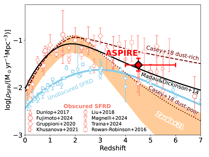
Figure 10: Obscured cosmic star formation rate density measured with the ASPIRE sample at $z=4-6$ (red diamond). For comparison we plot literature measurements of obscured SFRD as open salmon-pink symbols, including Rowan-Robinson et al. (2016), Dunlop et al. (2017), Liu et al. (2018), Gruppioni et al. (2020), Khusanova et al. (2021), Fujimoto et al. (2023), Magnelli et al. (2024) and Traina et al. (2024). Unobscured SFRD measured in rest-frame UV are shown as open sky-blue circles (including Reddy & Steidel 2009, Cucciati et al. 2012, Bouwens et al. 2015, Bouwens et al. 2020, Finkelstein et al. 2015, Alavi et al. 2016, Mehta et al. 2017, Moutard et al. 2020, Sun et al. 2023b) and the best-fit redshift-evolution model as indicated by the solid sky-blue curve. The Casey et al. (2018b) “dust-rich” and “dust-poor” scenarios are shown as dashed and dotted maroon lines, respectively. The inferred obscured SFRDs from a backward evolution model of 1–3 mm number counts (Zavala et al., 2021) are shown as orange shaded region. The solid black line shows the best-fit total SFRD from Madau & Dickinson (2014). Chabrier (2003) IMF has been assumed for all SFRD measurements in this plot.

4.4 Obscured Star-Formation Rate Density

We compute the obscured cosmic SFRD using the derived IRLF. Similar to Fujimoto et al. (2023), we integrate the IRLF down to $L_{\mathrm{IR}}=10^{10}$ $\mathrm{L}_{\odot}$, which corresponds to $\sim 0.0025L^{\star}$. Because of the flattening of IRLF toward the faint end, the integral of IRLF down to $L_{\mathrm{IR}}=10^{9}$ $\mathrm{L}_{\odot}$ is only higher than that down to $L_{\mathrm{IR}}=10^{10}$ $\mathrm{L}_{\odot}$ by $\sim 0.03$ dex. We convert the integral of IRLF to obscured SFRD using the factor listed in Section 3.2. We derive an obscured SFRD of $\log[\rho_{\mathrm{SFR,IR}}/($\mathrm{M}_{\odot}\,\mathrm{y}\mathrm{r}^{-1}\,\mathrm{M}\mathrm{p}\mathrm{c}^{-3}$)]=-1.52_{-0.13}^{+0.14}$ at $z=4-6$ (median $z=4.5$).

Figure 10 shows the obscured and unobscured SFRD measurements at $z\simeq 0-7$ in the literature, and the ASPIRE measurement is highlighted as the red diamond. At $z\gtrsim 4$, previous determinations of obscured SFRD are highly uncertain with a wide dispersion over 1-dex span (e.g., Rowan-Robinson et al., 2016; Dunlop et al., 2017; Koprowski et al., 2017; Liu et al., 2018; Gruppioni et al., 2020; Khusanova et al., 2021; Zavala et al., 2021; Magnelli et al., 2024; Traina et al., 2024). Our determination is within the dispersion of these previous measurements, and specifically, our measurement is about five times of the obscured SFRD derived by Zavala et al. (2021) through a backward modeling of millimeter number counts. As mentioned in Section 4.2, we caution the strong cosmic variance and void of $z>4$ DSFGs in the HUDF region that could affect the number counts at 1 and 3 mm used by Zavala et al. (2021). The uncertainty from far-IR SED can also lead to the error of SFRD determination with both the backward modeling method (Casey et al., 2018b; Zavala et al., 2021) and also our direct determination, which will be further discussed in Section 5.1.

We also compare our measurement with the so-called “dust-poor” and “dust-rich” scenarios of obscured SFRD evolution proposed by Casey et al. (2018b). Our result is in between these two model predictions at $z\sim 4.5$. The ASPIRE obscured SFRD is also comparable to the total SFRD (UV $+$ IR) at $z\sim 4.5$ from Madau & Dickinson (2014) best-fit model ($\log[\rho_{\mathrm{SFR,total}}/($\mathrm{M}_{\odot}\,\mathrm{y}\mathrm{r}^{-1}\,\mathrm{M}\mathrm{p}\mathrm{c}^{-3}$)]=-1.60$). Similar conclusion has also been drawn by recent ALCS observations (Fujimoto et al., 2023), suggesting that the total SFRD at $z=4-6$ could have been underestimated previously.

To understand the total amount and obscured fraction of SFRD at $z=4-6$, we compile the unobscured SFRD measurements from rest-frame UV surveys at $z=0-7$ (Reddy & Steidel, 2009; Cucciati et al., 2012; Bouwens et al., 2015, 2020; Finkelstein et al., 2015; Alavi et al., 2016; Mehta et al., 2017; Moutard et al., 2020; Sun et al., 2023b). Following Madau & Dickinson (2014), we fit the redshift evolution of unobscured SFRD with the following function:

$$\rho_{\mathrm{SFR,UV}}(z)=\Psi_{0}\frac{(\frac{1+z}{1+z_{0}})^{a}}{[1+(\frac{1+z}{1+z_{0}})^{b}]}\,$\mathrm{M}_{\odot}\,\mathrm{y}\mathrm{r}^{-1}\,\mathrm{M}\mathrm{p}\mathrm{c}^{-3}$$$ (4)

and we derive $z_{0}=3.74\pm 0.27$, $\log(\Psi_{0})=-1.37\pm 0.03$, $a=1.57\pm 0.16$ and $b=5.85\pm 0.33$. This implies an unobscured SFRD of $\log[\rho_{\mathrm{SFR,UV}}/($\mathrm{M}_{\odot}\,\mathrm{y}\mathrm{r}^{-1}\,\mathrm{M}\mathrm{p}\mathrm{c}^{-3}$)]=-1.80$ at $z\sim 4.5$, about half of the obscured SFRD as we derived based on ASPIRE data. Therefore, we conclude that $66_{-7}^{+7}$% of the total SFRD is obscured by dust at this epoch. The total SFRD that we derive is $\log[\rho_{\mathrm{SFR,total}}/($\mathrm{M}_{\odot}\,\mathrm{y}\mathrm{r}^{-1}\,\mathrm{M}\mathrm{p}\mathrm{c}^{-3}$)]=-1.34_{-0.08}^{+0.10}$, which is $180_{-30}^{+46}$% of the total SFRD from Madau & Dickinson (2014) best-fit model (similar to the conclusion in Fujimoto et al. 2023).

5 Discussion

In this section, we discuss the potential caveats of our determination of IRLF and SFRD. We also propose improvements that could be made through observations in the near future.

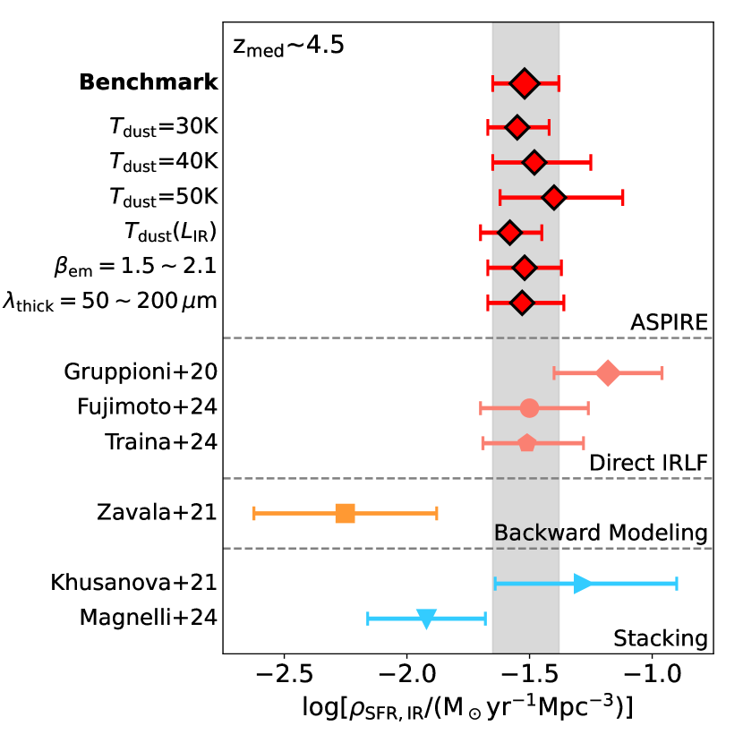
Figure 11: 16-50-84% credible-interval constraints of obscured SFRD at $z\sim 4.5$. Results from ASPIRE under various far-IR SED and dust temperature assumptions are shown on the top as solid red diamonds. Literature results through direct measurement and integral of IRLF are shown as salmon-pink symbols (Gruppioni et al., 2020; Fujimoto et al., 2023; Traina et al., 2024, interpolated to $z\sim 4.5$). The result from Zavala et al. (2021) through backward evolutionary modeling is shown as the orange square. Results based on stacking of ALMA data in bins of stellar masses or UV luminosities are shown in cyan triangles (Khusanova et al., 2021; Magnelli et al., 2024). The vertical gray band shows the 16–84% credible-interval of the “benchmark” obscured SFRD measured with ASPIRE.

5.1 Far-IR SED

In order to determine IRLF and SFRD, we make use of energy-balance SED fitting code cigale to derive $L_{\mathrm{IR}}$ (Section 3.2). The accuracy of $L_{\mathrm{IR}}$ thus rely on the validity of the energy-balance and far-IR SED assumptions.

It is known that DSFGs may not obey the energy-balance assumption along the observed sightline, simply because of patchy dust geometry. Previous studies have shown that DSFGs can have relatively blue UV continuum slopes, placing them above the $\mathrm{IRX}-\beta_{\mathrm{UV}}$ relation for normal star-forming galaxies (e.g., Penner et al., 2012; Oteo et al., 2013; Casey et al., 2014b). One of the most recent examples is HDF850.1 at $z=5.18$, which is $\sim$ 100 times above the $\mathrm{IRX}-\beta_{\mathrm{UV}}$ relation because of the leakage of UV photons (Sun et al., 2024). Similar effect has been seen for at least one DSFG in the ASPIRE sample (J0244m5008.C03), and the best-fit SED model does not reproduce the flux density in the F115W band satisfactorily (Figure 5).

To quantify the potential uncertainty of obscured SFRD determination with the energy balance assumption (hereafter the “benchmark” SFRD), we derive IRLF and obscured SFRD following the same methods presented in Section 4 but assuming different dust temperatures.

First of all, the cigale best-fit $L_{\mathrm{IR}}$ used by “benchmark” SFRD is roughly equivalent to that computed from modified black body SED with $T_{\mathrm{dust}}=33$ K and $\beta_{\mathrm{em}}=1.8$. This is similar to the typical $T_{\mathrm{dust}}$ for galaxies with $L_{\mathrm{IR}}=10^{12}$ $\mathrm{L}_{\odot}$ observed out to $z\sim 4.5$ (Sun et al. 2022; also modeled with MBB SED with $\beta_{\mathrm{em}}=1.8$), in which the direct $T_{\mathrm{dust}}$ measurements were obtained through Herschel/SPIRE at 250–500  micron thanks to lensing magnification.

However, arguably there is no consensus of the typical $T_{\mathrm{dust}}$ for LIRGs at $z\sim 5$. On one hand, studies have suggested that $M_{\mathrm{star}}$-selected galaxies have higher dust temperatures at higher redshifts through the stacking of Herschel data (Magnelli et al. 2014; Schreiber et al. 2018; caution shall be taken for the large beam size up to $\sim$35″). Higher dust temperatures at higher redshifts is a natural consequence of warmer cosmic microwave background (CMB) heating. On the other, direct $T_{\mathrm{dust}}$ measurements of $L_{\mathrm{IR}}$-selected DSFGs also suggest no or weak redshift evolution of $T_{\mathrm{dust}}$ up to $z\sim 4.5$ (e.g., Dudzevičiūtė et al., 2020; Drew & Casey, 2022; Sun et al., 2022), and therefore the $T_{\mathrm{dust}}(z)$ evolution at fixed stellar mass can simply be a combined effect of the weak evolution of the $L_{\mathrm{IR}}–T_{\mathrm{dust}}$ relation and strong evolution of the so-called star-forming “main sequence”.

Nevertheless, we explore the possible $T_{\mathrm{dust}}$ range at 30 to 50 K, derive the $L_{\mathrm{IR}}$ for ASPIRE sources through these $T_{\mathrm{dust}}$ assumptions with Casey 2012 SED (MBB $\beta_{\mathrm{em}}=1.8$ and mid-IR $\alpha_{\mathrm{MIR}}=2.0$) and plot the resultant obscured SFRD measurements in Figure 11. With hotter $T_{\mathrm{dust}}$, the resultant obscured SFRD is larger because $L_{\mathrm{IR}}$ is proportional to $T_{\mathrm{dust}}^{4}$ (the Stefan–Boltzmann law). However, the increase of obscured SFRD is only 0.12 dex (despite with larger uncertainty) with $T_{\mathrm{dust}}=50$ K assumption compared with the “benchmark”. This is a consequence of flattened IRLF at the faint end. Note that we also consider CMB heating effect following da Cunha et al. (2013), while the effect is found to be small at $z\sim 5$ where CMB temperature $T_{\mathrm{CMB}}$ is 16 K ($L_{\mathrm{IR}}$ boost is $\lesssim$ 0.01 dex).

We also consider the very hot IR SED template of Haro 11, a local moderately low-metallicity galaxy that undergoes starburst. De Rossi et al. (2018) suggested that the IR SED of Haro 11 could resemble those of luminous DSFGs at $z=5-7$, many of which are quasar host galaxies (Lyu et al., 2017) or selected through single-dish telescopes including SPT (e.g., Strandet et al., 2016). With the Haro 11 SED assumption, all galaxies in our sample exhibit $L_{\mathrm{IR}}$ of ULIRGs, and thus we will not be able to constrain the faint-end slope of IRLF any more, and literature measurements will dominate the IRLF fitting. The resultant obscured SFRD is similar to that approximated by $T_{\mathrm{dust}}=50$ K (Figure 11).

We also derive $L_{\mathrm{IR}}$ using the $\lambda_{\mathrm{peak}}(L_{\mathrm{IR}})$ relation in Casey et al. (2018a), which is equivalent to:

$$T_{\mathrm{dust}}/$\mathrm{K}$=32.7\,[L_{\mathrm{IR}}/(10^{12}\,$\mathrm{L}_{\odot}$)]^{0.09}$$ (5)

under the adopted SED assumption, and the resultant SFRD is slightly lower than our “benchmark” by 0.05 dex because of the relatively low $L_{\mathrm{IR}}$ of ASPIRE DSFGs (mostly LIRGs).

We also experiment different assumptions of dust emissivity and rest-frame wavelength where the dust optical depth is unity, both of which were fixed in previous modeling ($\beta_{\mathrm{em}}=1.8$ and $\lambda_{\mathrm{thick}}=100$ $\mathrm{\SIUnitSymbolMicro m}$). We find that the change of $\beta_{\mathrm{em}}$ by $\pm 0.3$ will result in a variation of 0.02 dex for $\rho_{\mathrm{SFR,IR}}$, and the change of $\lambda_{\mathrm{thick}}$ by a factor of 2 will result in a variation of 0.07 dex. These variations are relatively insignificant compared with the uncertainty of SFRD.

Finally, we also consider the potential AGN contribution to the 1.2-mm ALMA continuum and thus far-IR SED. Given that we have ruled out the existence of bright point-like structure in NIRCam imaging ($>$ 27.6 AB mag at F356W, 10$\sigma$ limit), any AGNs must be dust-obscured if they exist in ASPIRE DSFGs. We make use of the AGN SED templates constructed by Lyu et al. (2017) and Lyu & Rieke (2018). At the F356W detection limit, AGN at $A_{V}<3$ cannot contribute to more than 25% of observed ALMA flux density, and thus our SFRD measurement remains valid. However, we cannot rule out the existence of AGN with larger $A_{V}$ that may contribute to the 1.2 mm flux density more significantly (e.g., Symeonidis et al., 2016; McKinney et al., 2021), although obscured AGNs are not required to interpret the observational characteristics of ASPIRE DSFGs. Obscured AGN contribution to the IR SEDs of $z=4-6$ (U)LIRGs will need to be quantified through future JWST/MIRI observations and far-IR missions.

In conclusion, we argue that our determination of obscured SFRD is relatively robust against largely unknown far-IR SEDs, which are only loosely constrained by ALMA photometry in just one band. The ASPIRE determinations of obscured SFRD, regardless of $T_{\mathrm{dust}}$ assumptions, are all higher than that of Zavala et al. (2021) but consistent with recent direct measurements from Fujimoto et al. (2023) and Traina et al. (2024), and exhibit smaller uncertainties than literature measurements relying on stacked ALMA data (Khusanova et al., 2021; Magnelli et al., 2024). To further improve the accuracy of obscured SFRD determination, direct $T_{\mathrm{dust}}$ measurements through high-frequency ALMA continuum observations of $z>4$ DSFGs would be very helpful (e.g., Faisst et al., 2020; Mitsuhashi et al., 2023; Valentino et al., 2024; Villanueva et al., 2024).

Figure 12: The contribution to obscured cosmic SFRD at $z=4-6$ from sub-LIRGs, LIRGs, ULIRGs and HyLIRGs at $L_{\mathrm{IR}}$ from $10^{10}-10^{14}$ $\mathrm{L}_{\odot}$. LIRGs and ULIRGs at $L_{\mathrm{IR}}=10^{11}-10^{13}$ $\mathrm{L}_{\odot}$ contribute to the majority ($81_{-21}^{+11}$%) of obscured SFRD at this epoch.

5.2 The IRLF at the Bright End

Because of limited survey area, our ASPIRE DSFG sample cannot constrain the IRLF at the bright end (i.e., $L_{\mathrm{IR}}>L_{\mathrm{IR}}^{\star}\sim 10^{12.6}$ $\mathrm{L}_{\odot}$) in a self-contained manner. Therefore, we have to include literature measurements in our fitting, which could lead to the concern of $z_{\mathrm{spec}}$ completeness and $z_{\mathrm{phot}}$ validity.

Figure 12 shows the contribution to the obscured cosmic SFRD at $z=4-6$ by DSFGs in four $L_{\mathrm{IR}}$ bins, namely sub-LIRGs ($10^{10}\,\mbox{$\mathrm{L}_{\odot}$}\leq L_{\mathrm{IR}}<10^{11}\,\mbox{$\mathrm{L}_{\odot}$}$), LIRGs, ULIRGs and HyLIRGs ($10^{13}\,\mbox{$\mathrm{L}_{\odot}$}\leq L_{\mathrm{IR}}<10^{14}\,\mbox{$\mathrm{L}_{\odot}$}$). It is evident that both LIRGs and ULIRGs contribute to the majority ($81_{-21}^{+11}$%) of the obscured SFRD at this epoch. However, the contribution from ULIRGs is subject to a relatively large uncertainty ($44\pm 14$%) because of the uncertainty of IRLF at the bright end.

Although the spectroscopic completeness of literature measurement could be a concern, we argue that the derived $z=4-6$ IRLF in Section 8 is actually comparable to recent spectroscopic evidence. Simply considering GN10 ($z=5.30$; Riechers et al. 2020) and HDF850.1 ($z=5.18$; Walter et al. 2012) whose H$\alpha$ lines are detected through FRESCO NIRCam WFSS in the F444W band (Sun et al. 2024; see also Herard-Demanche et al. 2023; Xiao et al. 2023a), we can roughly estimate a volume density of $\Phi=10^{-5.0\pm 0.4}$ $\mathrm{M}\mathrm{p}\mathrm{c}^{-3}\,\mathrm{d}\mathrm{e}\mathrm{x}^{-1}$ (cosmic variance considered) within the luminosity bin $10^{12.5}-10^{13.1}$ $\mathrm{L}_{\odot}$ assuming the FRESCO survey volume at $z=4.9-6.0$. This is consistent with the volume density expected from our best-fit IRLF at the bin center ($\Phi=10^{-5.4}$ $\mathrm{M}\mathrm{p}\mathrm{c}^{-3}\,\mathrm{d}\mathrm{e}\mathrm{x}^{-1}$). However, we also note that both galaxies reside in a complex overdense environment (Calvi et al., 2021, 2023; Herard-Demanche et al., 2023; Sun et al., 2024), and there could be more galaxies in both GOODS field that could contribute to the volume density (Xiao et al., 2023a).

In JWST Cycle-3, there are four planned large / treasury NIRCam WFSS surveys over much larger volumes, including NEXUS (PID: 5105, PI: Shen, Y.; Shen et al. 2024), COSMOS-3D (PID: 5893, PI: Kakiichi, K.), POPPIES (PID: 5398, PI: Kartaltepe, J.), SAPPHIRES (PID: 6434, PI: Egami, E.), totaling more than one thousand hours of JWST time. These observations, in synergy with obtained / planned (sub-)millimeter surveys in cosmological deep fields (COSMOS, including Casey et al. 2013, 2021; Geach et al. 2017; Wang et al. 2017; Simpson et al. 2019; and NEP, including Shim et al. 2020; Hyun et al. 2023), will provide powerful and essential spectroscopy of high-redshift DSFGs at the bright end of IRLF, constraining the obscured cosmic star-formation history towards the Epoch of Reionization with unprecedented accuracy.

6 Summary

In this paper, we present a stringent measurement of the dust-obscured SFRD at $z=4-6$ through the ASPIRE JWST and ALMA survey. ASPIRE obtained JWST NIRCam WFSS survey at 3.1–4.0 $\mathrm{\SIUnitSymbolMicro m}$ and ALMA mosaics at 1.2 mm along 25 quasar sightlines. We make use of this JWST and ALMA dataset to identify DSFGs at $z_{\mathrm{spec}}=4-6$ through ALMA continuum detections and JWST spectroscopy. The main results are summarized as follows:

1. We identify eight DSFGs at $z_{\mathrm{spec}}=4-6$ through the detections of H$\alpha$ (for seven sources at $z=4.07-4.80$) or [O III] $\lambda$5008 (for one source at $z=5.55$) lines with NIRCam WFSS. These DSFGs are discovered in seven out of 25 ASPIRE quasar fields totaling a survey area of $\sim$ 35 arcmin². For six DSFGs, we also detect at least one more faint lines such as H$\beta$, [O III] $\lambda$4960, [N II] $\lambda$6585 and [S II] $\lambda\lambda$6718,6733.

2. We conduct energy-balance SED modeling of these DSFGs through JWST and ALMA photometry (four bands in total). The median stellar mass is $\log(M_{\mathrm{star}}/$\mathrm{M}_{\odot}$)=10.3\pm 0.2$, and the median IR luminosity is $\log(L_{\mathrm{IR}}/$\mathrm{L}_{\odot}$)=11.7\pm 0.1$.

3. 96$\pm$2% of the star formation in $z\sim 5$ DSFGs probed by ASPIRE are obscured by dust. However, the escape fractions of H$\alpha$ photon is anti-correlated with their IR luminosities, resulting in an almost constant H$\alpha$ luminosity across 2-dex wide span of $L_{\mathrm{IR}}$, which is also well above the $5\sigma$ detection limit with NIRCam WFSS. We observe a typical $\tau_{\mathrm{UV}}/\tau_{\mathrm{H\alpha}}$ ratio of $1.61\pm 0.34$ for $z\sim 5$ DSFGs, slightly higher than that of local starburst, which could lead to an enhanced H$\alpha$ visibility in these $z\sim 5$ DSFGs.

4. We obtain 1.2-mm number count of DSFGs at $z=4-6$, finding it higher than previous determination based on ALMA Cycle-4 large program ASPECS (Popping et al., 2020; Zavala et al., 2021) but similar to that from ALMA Cycle-5 large program ALPINE (Gruppioni et al., 2020). We argue that our measurement is robust against cosmic variance (shot noise) because of averaging 25 independent sightlines, while the ASPECS survey in the HUDF region encounters a void of DSFGs at $z=4-6$ because of strong shot noise.

5. We obtain spectroscopically complete measurement of the infrared luminosity function at $z=4-6$ down to $L_{\mathrm{IR}}\sim 2\times 10^{11}$ $\mathrm{L}_{\odot}$. We observe a flattening of the faint-end slope ($\alpha=0.59_{-0.45}^{+0.39}$) of the IRLF. Our measurements are consistent with previous measurements including Gruppioni et al. (2020), Fujimoto et al. (2023) and Traina et al. (2024) at the faint end (with spectroscopic incompleteness), but slightly lower than a few model predictions.

6. We derive an obscured SFRD of $\log[\rho_{\mathrm{SFR,IR}}/($\mathrm{M}_{\odot}\,\mathrm{y}\mathrm{r}^{-1}\,\mathrm{M}\mathrm{p}\mathrm{c}^{-3}$)]=-1.52_{-0.13}^{+0.14}$ at $z=4-6$ (median $z=4.5$). This is comparable to the total (obscured and unobscured) SFRD modeled by Madau & Dickinson (2014), suggesting that the majority ($66_{-7}^{+7}$%) of the total SFRD is obscured by dust at this epoch. Our measurement is similar to that of direct measurements with recent literature (e.g., Fujimoto et al., 2023; Traina et al., 2024), but $\sim$ 5 times higher than that of Zavala et al. (2021) through a backward evolutionary modeling.

7. We conclude that our measurement of SFRD is relatively robust against uncertainty in far-IR SED shape (primarily dust temperature). Future ALMA high-frequency observations will be helpful to determine the dust temperature and improve the accuracy of obscured SFRD. Although our result suggests the majority ($81_{-21}^{+11}$%) of obscured SFRD is contributed by both LIRGs and ULIRGs, the current uncertainty at the bright end of IRLF (especially $z_{\mathrm{spec}}$ incompleteness) will need to be resolved with planned JWST NIRCam WFSS surveys over much larger volume.

Appendix A Lensing Magnification

The highest-redshift source in our sample, J0109m3047.C02 ($z=5.549$) is very close to a foreground galaxy (separation $\sim$ 0$\farcs$8). J0109m3047.C02 is also extended in morphology along the tangential direction to this foreground galaxy, indicating that J0109m3047.C02 is strongly lensed by the foreground source. To correctly account for the lensing effect in the analyses of its physical properties and lensing bias in the determination of LF, we model the lensing magnification through the following steps.

We first obtain optical and near-IR photometry of the foreground lens. At optical wavelength, the foreground galaxy is much brighter than J0109m3047.C02 and the other bluer source to the northwest as seen in Figure 2. Therefore, we directly make use of DES DR2 (Abbott et al., 2021) photometry in $g$, $r$, $i$, $z$ and $Y$ band. At JWST/NIRCam wavelength, we carefully model the source morphology with galfit (Peng et al., 2010). Because J0109m3047.C02 appears clumpy in the image, we include ten components of Sérsic profiles or point-spread functions (PSFs) to model the complex image in F115W, F200W and F356W band. We make use of PSF model generated through webbpsf (Perrin et al., 2014). Except for the foreground lens component, the best-fit morphological models of other components are subtracted from the mosaicked images. We therefore obtain the near-IR aperture photometry of the foreground lens on the residual images (22.90$\pm$0.05, 21.82$\pm$0.04, 21.12$\pm$0.05 AB mag in F115W, F200W, F356W band, respectively).

Because no obvious emission or absorption line could be identified in the grism spectra of the foreground lens, we derive the photometric redshifts through SED modeling. We feed the photometric measurements into CIGALE (Boquien et al., 2019) with redshift grids from $z=0.5$ to 2.5 ($\Delta z$ = 0.05), and derive the reduced $\chi_{\mathrm{red}}^{2}(z)$ and stellar mass $M_{\mathrm{star}}$$(z)$ for each of the fitting. We derive the probability distribution of redshifts through $P(z)\propto\exp[-\chi_{\mathrm{red}}^{2}(z)/2]$ and normalization $\int_{0.5}^{2.5}P(z)dz=1$, and conclude a photometric redshift of $z_{\mathrm{phot}}$ = 1.18$\pm$0.05 for the foreground lens. At this redshift no strong hydrogen line is expected in the F356W grism spectrum, consistent with the aforementioned non-detection. We randomly draw redshifts from the $P(z)$ distribution, and then draw the corresponding $M_{\mathrm{star}}$ from the best-fit $M_{\mathrm{star}}$$(z)$ and the uncertainties. Assuming the stellar-mass Tully-Fisher Relation measured at $z\sim 1$ (Übler et al., 2017), we derive velocity dispersion ($\sigma_{v}$) for each of the drawn pairs of $z$ and $M_{\mathrm{star}}$. The median and $1\sigma$ uncertainty of velocity dispersion is $\sigma_{v}=150\pm 28$ $\mathrm{k}\mathrm{m}\,\mathrm{s}^{-1}$ for the foreground lens.

We then model the foreground lens using the drawn redshifts and $\sigma_{v}$ through software lenstool (Jullo et al., 2007). We assume a singular isothermal spherical distribution of matter in the foreground potential. We therefore derive a lensing magnification of $\mu=1.91\pm 0.50$ for the ALMA continuum source. However, we notice that differential lensing effect is seen for J0109m3047.C02 because its complex morphology at different wavelengths. The light-weighted (through image segments) magnification for J0109m3047.C02 in F115W, F200W and F356W band is $1.58\pm 0.33$, $1.54\pm 0.29$ and $1.53\pm 0.28$, respectively. These magnification factors have been corrected when we infer the physical properties (e.g., luminosity and mass) of J0109m3047.C02.

Appendix B Completeness Correction

We simulate ALMA observations with casa to derive the completeness correction at each ALMA source flux and S/N. First of all, we assume a 2D circular Gaussian profile for ALMA continuum source with an effective radius $R_{\mathrm{e}}=0\farcs 23$ (i.e., 1.5 kpc at $z=4.5$). This is consistent with the sizes that we measured from image-plane fitting (with casa imfit) for ASPIRE DSFGs detected at $z=4-6$ and $\mathrm{S/N}>10$. We scale the surface brightness profile such that the total flux density is 0.10–1.0 mJy at 1.2 mm in each of our run of simulations. ALMA continuum observation measurement sets are then simulated through casa simobserve command with the same configuration and similar observing condition (exposure time and precipitated water vapor) as those of actual ASPIRE observations. With each input flux density, we simulate the observations for 100 times, produce the continuum images at both native and 1$\farcs$0-tapered resolution with the same pipeline adopted for real data. We then identify peaks in simulated images within 1″ from the injected source position. The detection criteria are the same as those adopted in Section 2.2.

Figure B1: Completeness as a function of ALMA flux density on 1$\farcs$0 uv-tapered images (before primary beam response correction). Best-fit error function is shown as the solid black line.

At each injected source flux density, we compute the fraction of sources in simulated images that are above our detection threshold. Such a fraction is therefore considered as the survey completeness at the injected source flux, and Figure B1 shows the completeness as a function of ALMA flux density on the tapered images. We also conduct statistics on native-resolution images, but the results are less relevant because all of the ASPIRE DSFGs $z=4-6$ exhibit higher S/N on tapered images than native images (and thus completeness is higher). We fit the measured completeness with an error function:

$$C(f)=\frac{1}{2}\mathrm{erf}\big{(}\frac{S-S_{0}}{\sigma}\big{)}+\frac{1}{2}$$ (B1)

and we find that the completeness is 50% at source flux density $S=S_{0}=0.143\pm 0.003$ mJy. All ASPIRE DSFGs at $z=4-6$ show high completeness ($C\sim 1$) because of their high fidelity of detections ($S_{\mathrm{1.2mm}}\geq 0.24$ mJy and $\mathrm{S/N}\geq 6.5$). We also rewrite the completeness function in terms of ALMA source S/N and use it for the IRLF completeness calculation.

Through our injection and detection experiment, we also verify the 1.1$\times$ scaling factor applied to the peak flux density measured on tapered image ($f_{\mathrm{tap}}$; Section 3.1). We also conclude negligible flux boosting effect (e.g., Eddington bias; $<$3% through our simulations) in the S/N and flux density range of our targets.

References

- Abbott et al. (2021) Abbott, T. M. C., Adamów, M., Aguena, M., et al. 2021, ApJS, 255, 20, doi: 10.3847/1538-4365/ac00b3
- Adscheid et al. (2024) Adscheid, S., Magnelli, B., Liu, D., et al. 2024, A&A, 685, A1, doi: 10.1051/0004-6361/202348407
- Alavi et al. (2016) Alavi, A., Siana, B., Richard, J., et al. 2016, ApJ, 832, 56, doi: 10.3847/0004-637X/832/1/56
- Alcalde Pampliega et al. (2019) Alcalde Pampliega, B., Pérez-González, P. G., Barro, G., et al. 2019, ApJ, 876, 135, doi: 10.3847/1538-4357/ab14f2
- Algera et al. (2023) Algera, H. S. B., Inami, H., Oesch, P. A., et al. 2023, MNRAS, 518, 6142, doi: 10.1093/mnras/stac3195
- Aravena et al. (2020) Aravena, M., Boogaard, L., Gónzalez-López, J., et al. 2020, arXiv e-prints, arXiv:2006.04284. https://arxiv.org/abs/2006.04284
- Armus et al. (2009) Armus, L., Mazzarella, J. M., Evans, A. S., et al. 2009, PASP, 121, 559, doi: 10.1086/600092
- Arnouts & Ilbert (2011) Arnouts, S., & Ilbert, O. 2011, LePHARE: Photometric Analysis for Redshift Estimate, Astrophysics Source Code Library, record ascl:1108.009
- Astropy Collaboration et al. (2013) Astropy Collaboration, Robitaille, T. P., Tollerud, E. J., et al. 2013, A&A, 558, A33, doi: 10.1051/0004-6361/201322068
- Astropy Collaboration et al. (2018) Astropy Collaboration, Price-Whelan, A. M., Sipőcz, B. M., et al. 2018, AJ, 156, 123, doi: 10.3847/1538-3881/aabc4f
- Bañados et al. (2021) Bañados, E., Mazzucchelli, C., Momjian, E., et al. 2021, ApJ, 909, 80, doi: 10.3847/1538-4357/abe239
- Barrufet et al. (2024) Barrufet, L., Oesch, P., Marques-Chaves, R., et al. 2024, arXiv e-prints, arXiv:2404.08052, doi: 10.48550/arXiv.2404.08052
- Bauer et al. (2004) Bauer, F. E., Alexander, D. M., Brandt, W. N., et al. 2004, AJ, 128, 2048, doi: 10.1086/424859
- Béthermin et al. (2017) Béthermin, M., Wu, H.-Y., Lagache, G., et al. 2017, A&A, 607, A89, doi: 10.1051/0004-6361/201730866
- Béthermin et al. (2020) Béthermin, M., Fudamoto, Y., Ginolfi, M., et al. 2020, A&A, 643, A2, doi: 10.1051/0004-6361/202037649
- Béthermin et al. (2022) Béthermin, M., Gkogkou, A., Van Cuyck, M., et al. 2022, A&A, 667, A156, doi: 10.1051/0004-6361/202243888
- Bik et al. (2024) Bik, A., Álvarez-Márquez, J., Colina, L., et al. 2024, A&A, 686, A3, doi: 10.1051/0004-6361/202348845
- Boogaard et al. (2024) Boogaard, L. A., Gillman, S., Melinder, J., et al. 2024, ApJ, 969, 27, doi: 10.3847/1538-4357/ad43e5
- Boquien et al. (2019) Boquien, M., Burgarella, D., Roehlly, Y., et al. 2019, A&A, 622, A103, doi: 10.1051/0004-6361/201834156
- Bouwens et al. (2020) Bouwens, R., González-López, J., Aravena, M., et al. 2020, ApJ, 902, 112, doi: 10.3847/1538-4357/abb830
- Bouwens et al. (2015) Bouwens, R. J., Illingworth, G. D., Oesch, P. A., et al. 2015, ApJ, 811, 140, doi: 10.1088/0004-637X/811/2/140
- Bradley et al. (2024) Bradley, L., Sipőcz, B., Robitaille, T., et al. 2024, astropy/photutils: 1.12.0, 1.12.0, Zenodo, doi: 10.5281/zenodo.10967176
- Bruzual & Charlot (2003) Bruzual, G., & Charlot, S. 2003, MNRAS, 344, 1000, doi: 10.1046/j.1365-8711.2003.06897.x
- Burgarella et al. (2013) Burgarella, D., Buat, V., Gruppioni, C., et al. 2013, A&A, 554, A70, doi: 10.1051/0004-6361/201321651
- Bushouse et al. (2023) Bushouse, H., Eisenhamer, J., Dencheva, N., et al. 2023, JWST Calibration Pipeline, 1.10.2, Zenodo, doi: 10.5281/zenodo.7829329
- Calvi et al. (2023) Calvi, R., Castignani, G., & Dannerbauer, H. 2023, arXiv e-prints, arXiv:2302.10323, doi: 10.48550/arXiv.2302.10323
- Calvi et al. (2021) Calvi, R., Dannerbauer, H., Arrabal Haro, P., et al. 2021, MNRAS, 502, 4558, doi: 10.1093/mnras/staa4037
- Calzetti (1997) Calzetti, D. 1997, in American Institute of Physics Conference Series, Vol. 408, The ultraviolet universe at low and High redshift, ed. W. H. Waller (AIP), 403–412, doi: 10.1063/1.53764
- Calzetti et al. (2000) Calzetti, D., Armus, L., Bohlin, R. C., et al. 2000, ApJ, 533, 682, doi: 10.1086/308692
- Caputi et al. (2012) Caputi, K. I., Dunlop, J. S., McLure, R. J., et al. 2012, ApJ, 750, L20, doi: 10.1088/2041-8205/750/1/L20
- CASA Team et al. (2022) CASA Team, Bean, B., Bhatnagar, S., et al. 2022, PASP, 134, 114501, doi: 10.1088/1538-3873/ac9642
- Casey (2012) Casey, C. M. 2012, MNRAS, 425, 3094, doi: 10.1111/j.1365-2966.2012.21455.x
- Casey et al. (2018a) Casey, C. M., Hodge, J., Zavala, J. A., et al. 2018a, ApJ, 862, 78, doi: 10.3847/1538-4357/aacd11
- Casey et al. (2014a) Casey, C. M., Narayanan, D., & Cooray, A. 2014a, Phys. Rep., 541, 45, doi: 10.1016/j.physrep.2014.02.009
- Casey et al. (2013) Casey, C. M., Chen, C.-C., Cowie, L. L., et al. 2013, MNRAS, 436, 1919, doi: 10.1093/mnras/stt1673
- Casey et al. (2014b) Casey, C. M., Scoville, N. Z., Sanders, D. B., et al. 2014b, ApJ, 796, 95, doi: 10.1088/0004-637X/796/2/95
- Casey et al. (2018b) Casey, C. M., Zavala, J. A., Spilker, J., et al. 2018b, ApJ, 862, 77, doi: 10.3847/1538-4357/aac82d
- Casey et al. (2019) Casey, C. M., Zavala, J. A., Aravena, M., et al. 2019, ApJ, 887, 55, doi: 10.3847/1538-4357/ab52ff
- Casey et al. (2021) Casey, C. M., Zavala, J. A., Manning, S. M., et al. 2021, ApJ, 923, 215, doi: 10.3847/1538-4357/ac2eb4
- Chabrier (2003) Chabrier, G. 2003, PASP, 115, 763, doi: 10.1086/376392
- Champagne et al. (2024a) Champagne, J. B., Wang, F., Zhang, H., et al. 2024a, arXiv e-prints, arXiv:2410.03826, doi: 10.48550/arXiv.2410.03826
- Champagne et al. (2024b) Champagne, J. B., Wang, F., Yang, J., et al. 2024b, arXiv e-prints, arXiv:2410.03827, doi: 10.48550/arXiv.2410.03827
- Chary & Elbaz (2001) Chary, R., & Elbaz, D. 2001, ApJ, 556, 562, doi: 10.1086/321609
- Chen et al. (2022) Chen, C.-C., Liao, C.-L., Smail, I., et al. 2022, ApJ, 929, 159, doi: 10.3847/1538-4357/ac61df
- Chen et al. (2023) Chen, J., Ivison, R. J., Zwaan, M. A., et al. 2023, MNRAS, 518, 1378, doi: 10.1093/mnras/stac2989
- Colina et al. (2023) Colina, L., Crespo Gómez, A., Álvarez-Márquez, J., et al. 2023, A&A, 673, L6, doi: 10.1051/0004-6361/202346535
- Cooper et al. (2024) Cooper, O. R., Brammer, G., Heintz, K. E., et al. 2024, arXiv e-prints, arXiv:2410.08387, doi: 10.48550/arXiv.2410.08387
- Cowie et al. (2002) Cowie, L. L., Garmire, G. P., Bautz, M. W., et al. 2002, ApJ, 566, L5, doi: 10.1086/339545
- Cucciati et al. (2012) Cucciati, O., Tresse, L., Ilbert, O., et al. 2012, A&A, 539, A31, doi: 10.1051/0004-6361/201118010
- da Cunha et al. (2013) da Cunha, E., Groves, B., Walter, F., et al. 2013, ApJ, 766, 13, doi: 10.1088/0004-637X/766/1/13
- da Cunha et al. (2015) da Cunha, E., Walter, F., Smail, I. R., et al. 2015, ApJ, 806, 110, doi: 10.1088/0004-637X/806/1/110
- De Rossi et al. (2018) De Rossi, M. E., Rieke, G. H., Shivaei, I., Bromm, V., & Lyu, J. 2018, ApJ, 869, 4, doi: 10.3847/1538-4357/aaebf8
- Decarli et al. (2017) Decarli, R., Walter, F., Venemans, B. P., et al. 2017, Nature, 545, 457, doi: 10.1038/nature22358
- Dey et al. (2019) Dey, A., Schlegel, D. J., Lang, D., et al. 2019, AJ, 157, 168, doi: 10.3847/1538-3881/ab089d
- Drew & Casey (2022) Drew, P. M., & Casey, C. M. 2022, arXiv e-prints, arXiv:2203.16655. https://arxiv.org/abs/2203.16655
- Driver & Robotham (2010) Driver, S. P., & Robotham, A. S. G. 2010, MNRAS, 407, 2131, doi: 10.1111/j.1365-2966.2010.17028.x
- Dudzevičiūtė et al. (2020) Dudzevičiūtė, U., Smail, I., Swinbank, A. M., et al. 2020, MNRAS, 494, 3828, doi: 10.1093/mnras/staa769
- Dunlop et al. (2017) Dunlop, J. S., McLure, R. J., Biggs, A. D., et al. 2017, MNRAS, 466, 861, doi: 10.1093/mnras/stw3088
- Enia et al. (2022) Enia, A., Talia, M., Pozzi, F., et al. 2022, ApJ, 927, 204, doi: 10.3847/1538-4357/ac51ca
- Faisst et al. (2020) Faisst, A. L., Fudamoto, Y., Oesch, P. A., et al. 2020, MNRAS, 498, 4192, doi: 10.1093/mnras/staa2545
- Finkelstein et al. (2015) Finkelstein, S. L., Ryan, Russell E., J., Papovich, C., et al. 2015, ApJ, 810, 71, doi: 10.1088/0004-637X/810/1/71
- Foreman-Mackey et al. (2013) Foreman-Mackey, D., Hogg, D. W., Lang, D., & Goodman, J. 2013, PASP, 125, 306, doi: 10.1086/670067
- Franco et al. (2018) Franco, M., Elbaz, D., Béthermin, M., et al. 2018, A&A, 620, A152, doi: 10.1051/0004-6361/201832928
- Fudamoto et al. (2020) Fudamoto, Y., Oesch, P. A., Faisst, A., et al. 2020, A&A, 643, A4, doi: 10.1051/0004-6361/202038163
- Fudamoto et al. (2021) Fudamoto, Y., Oesch, P. A., Schouws, S., et al. 2021, Nature, 597, 489, doi: 10.1038/s41586-021-03846-z
- Fujimoto et al. (2016) Fujimoto, S., Ouchi, M., Ono, Y., et al. 2016, ApJS, 222, 1, doi: 10.3847/0067-0049/222/1/1
- Fujimoto et al. (2023) Fujimoto, S., Kohno, K., Ouchi, M., et al. 2023, arXiv e-prints, arXiv:2303.01658, doi: 10.48550/arXiv.2303.01658
- Gaia Collaboration et al. (2023) Gaia Collaboration, Vallenari, A., Brown, A. G. A., et al. 2023, A&A, 674, A1, doi: 10.1051/0004-6361/202243940
- García-Marín et al. (2009) García-Marín, M., Colina, L., & Arribas, S. 2009, A&A, 505, 1017, doi: 10.1051/0004-6361/200912537
- Gardner et al. (2023) Gardner, J. P., Mather, J. C., Abbott, R., et al. 2023, PASP, 135, 068001, doi: 10.1088/1538-3873/acd1b5
- Geach et al. (2017) Geach, J. E., Dunlop, J. S., Halpern, M., et al. 2017, MNRAS, 465, 1789, doi: 10.1093/mnras/stw2721
- Gehrels (1986) Gehrels, N. 1986, ApJ, 303, 336, doi: 10.1086/164079
- Giménez-Arteaga et al. (2022) Giménez-Arteaga, C., Brammer, G. B., Marchesini, D., et al. 2022, ApJS, 263, 17, doi: 10.3847/1538-4365/ac958c
- Gómez-Guijarro et al. (2022) Gómez-Guijarro, C., Elbaz, D., Xiao, M., et al. 2022, A&A, 658, A43, doi: 10.1051/0004-6361/202141615
- González-López et al. (2020) González-López, J., Novak, M., Decarli, R., et al. 2020, arXiv e-prints, arXiv:2002.07199. https://arxiv.org/abs/2002.07199
- Gordon et al. (2003) Gordon, K. D., Clayton, G. C., Misselt, K. A., Landolt, A. U., & Wolff, M. J. 2003, ApJ, 594, 279, doi: 10.1086/376774
- Gottumukkala et al. (2024) Gottumukkala, R., Barrufet, L., Oesch, P. A., et al. 2024, MNRAS, 530, 966, doi: 10.1093/mnras/stae754
- Gruppioni et al. (2013) Gruppioni, C., Pozzi, F., Rodighiero, G., et al. 2013, MNRAS, 432, 23, doi: 10.1093/mnras/stt308
- Gruppioni et al. (2020) Gruppioni, C., Béthermin, M., Loiacono, F., et al. 2020, A&A, 643, A8, doi: 10.1051/0004-6361/202038487
- Hatsukade et al. (2018) Hatsukade, B., Kohno, K., Yamaguchi, Y., et al. 2018, PASJ, 70, 105, doi: 10.1093/pasj/psy104
- Herard-Demanche et al. (2023) Herard-Demanche, T., Bouwens, R. J., Oesch, P. A., et al. 2023, arXiv e-prints, arXiv:2309.04525, doi: 10.48550/arXiv.2309.04525
- Hodge & da Cunha (2020) Hodge, J. A., & da Cunha, E. 2020, Royal Society Open Science, 7, 200556, doi: 10.1098/rsos.200556
- Horne (1986) Horne, K. 1986, PASP, 98, 609, doi: 10.1086/131801
- Huang et al. (2011) Huang, J. S., Zheng, X. Z., Rigopoulou, D., et al. 2011, ApJ, 742, L13, doi: 10.1088/2041-8205/742/1/L13
- Hughes et al. (1998) Hughes, D. H., Serjeant, S., Dunlop, J., et al. 1998, Nature, 394, 241, doi: 10.1038/28328
- Hyun et al. (2023) Hyun, M., Im, M., Smail, I. R., et al. 2023, ApJS, 264, 19, doi: 10.3847/1538-4365/ac9bf4
- Jin et al. (2019a) Jin, J.-J., Zhu, Y.-N., Wu, H., et al. 2019a, ApJS, 244, 33, doi: 10.3847/1538-4365/ab3bfe
- Jin et al. (2019b) Jin, S., Daddi, E., Magdis, G. E., et al. 2019b, ApJ, 887, 144, doi: 10.3847/1538-4357/ab55d6
- Jin et al. (2024a) Jin, S., Sillassen, N. B., Hodge, J., et al. 2024a, arXiv e-prints, arXiv:2407.07585, doi: 10.48550/arXiv.2407.07585
- Jin et al. (2024b) Jin, X., Yang, J., Fan, X., et al. 2024b, arXiv e-prints, arXiv:2410.01318, doi: 10.48550/arXiv.2410.01318
- Jullo et al. (2007) Jullo, E., Kneib, J. P., Limousin, M., et al. 2007, New Journal of Physics, 9, 447, doi: 10.1088/1367-2630/9/12/447
- Kennicutt (1998) Kennicutt, Robert C., J. 1998, ARA&A, 36, 189, doi: 10.1146/annurev.astro.36.1.189
- Kepley et al. (2020) Kepley, A. A., Tsutsumi, T., Brogan, C. L., et al. 2020, PASP, 132, 024505, doi: 10.1088/1538-3873/ab5e14
- Khusanova et al. (2021) Khusanova, Y., Bethermin, M., Le Fèvre, O., et al. 2021, A&A, 649, A152, doi: 10.1051/0004-6361/202038944
- Kohno et al. (2023) Kohno, K., Fujimoto, S., Tsujita, A., et al. 2023, arXiv e-prints, arXiv:2305.15126, doi: 10.48550/arXiv.2305.15126
- Kokorev et al. (2022) Kokorev, V., Brammer, G., Fujimoto, S., et al. 2022, ApJS, 263, 38, doi: 10.3847/1538-4365/ac9909
- Koprowski et al. (2017) Koprowski, M. P., Dunlop, J. S., Michałowski, M. J., et al. 2017, MNRAS, 471, 4155, doi: 10.1093/mnras/stx1843
- Lagos et al. (2020) Lagos, C. d. P., da Cunha, E., Robotham, A. S. G., et al. 2020, MNRAS, 499, 1948, doi: 10.1093/mnras/staa2861
- Le Fèvre et al. (2020) Le Fèvre, O., Béthermin, M., Faisst, A., et al. 2020, A&A, 643, A1, doi: 10.1051/0004-6361/201936965
- Lim et al. (2020) Lim, C.-F., Wang, W.-H., Smail, I., et al. 2020, ApJ, 889, 80, doi: 10.3847/1538-4357/ab607f
- Ling et al. (2024) Ling, C., Sun, B., Cheng, C., et al. 2024, arXiv e-prints, arXiv:2402.16649, doi: 10.48550/arXiv.2402.16649
- Liu et al. (2018) Liu, D., Daddi, E., Dickinson, M., et al. 2018, ApJ, 853, 172, doi: 10.3847/1538-4357/aaa600
- Lyu & Rieke (2018) Lyu, J., & Rieke, G. H. 2018, ApJ, 866, 92, doi: 10.3847/1538-4357/aae075
- Lyu et al. (2017) Lyu, J., Rieke, G. H., & Shi, Y. 2017, ApJ, 835, 257, doi: 10.3847/1538-4357/835/2/257
- Madau & Dickinson (2014) Madau, P., & Dickinson, M. 2014, ARA&A, 52, 415, doi: 10.1146/annurev-astro-081811-125615
- Magnelli et al. (2014) Magnelli, B., Lutz, D., Saintonge, A., et al. 2014, A&A, 561, A86, doi: 10.1051/0004-6361/201322217
- Magnelli et al. (2024) Magnelli, B., Adscheid, S., Wang, T.-M., et al. 2024, arXiv e-prints, arXiv:2405.18086, doi: 10.48550/arXiv.2405.18086
- Manning et al. (2022) Manning, S. M., Casey, C. M., Zavala, J. A., et al. 2022, ApJ, 925, 23, doi: 10.3847/1538-4357/ac366a
- Mazzucchelli et al. (2019) Mazzucchelli, C., Decarli, R., Farina, E. P., et al. 2019, ApJ, 881, 163, doi: 10.3847/1538-4357/ab2f75
- McKinney et al. (2021) McKinney, J., Hayward, C. C., Rosenthal, L. J., et al. 2021, ApJ, 921, 55, doi: 10.3847/1538-4357/ac185f
- McKinney et al. (2023a) McKinney, J., Manning, S. M., Cooper, O. R., et al. 2023a, ApJ, 956, 72, doi: 10.3847/1538-4357/acf614
- McKinney et al. (2023b) McKinney, J., Finnerty, L., Casey, C. M., et al. 2023b, ApJ, 946, L39, doi: 10.3847/2041-8213/acc322
- McKinney et al. (2024) McKinney, J., Casey, C. M., Long, A. S., et al. 2024, arXiv e-prints, arXiv:2408.08346, doi: 10.48550/arXiv.2408.08346
- McMullin et al. (2007) McMullin, J. P., Waters, B., Schiebel, D., Young, W., & Golap, K. 2007, in Astronomical Society of the Pacific Conference Series, Vol. 376, Astronomical Data Analysis Software and Systems XVI, ed. R. A. Shaw, F. Hill, & D. J. Bell, 127
- Mehta et al. (2017) Mehta, V., Scarlata, C., Rafelski, M., et al. 2017, ApJ, 838, 29, doi: 10.3847/1538-4357/aa6259
- Meurer et al. (1999) Meurer, G. R., Heckman, T. M., & Calzetti, D. 1999, ApJ, 521, 64, doi: 10.1086/307523
- Mitsuhashi et al. (2023) Mitsuhashi, I., Harikane, Y., Bauer, F. E., et al. 2023, arXiv e-prints, arXiv:2311.16857, doi: 10.48550/arXiv.2311.16857
- Moretti et al. (2003) Moretti, A., Campana, S., Lazzati, D., & Tagliaferri, G. 2003, ApJ, 588, 696, doi: 10.1086/374335
- Moster et al. (2011) Moster, B. P., Somerville, R. S., Newman, J. A., & Rix, H.-W. 2011, ApJ, 731, 113, doi: 10.1088/0004-637X/731/2/113
- Moutard et al. (2020) Moutard, T., Sawicki, M., Arnouts, S., et al. 2020, MNRAS, 494, 1894, doi: 10.1093/mnras/staa706
- Nguyen et al. (2010) Nguyen, H. T., Schulz, B., Levenson, L., et al. 2010, A&A, 518, L5, doi: 10.1051/0004-6361/201014680
- Noll et al. (2009) Noll, S., Burgarella, D., Giovannoli, E., et al. 2009, A&A, 507, 1793, doi: 10.1051/0004-6361/200912497
- Oesch et al. (2007) Oesch, P. A., Stiavelli, M., Carollo, C. M., et al. 2007, ApJ, 671, 1212, doi: 10.1086/522423
- Oesch et al. (2023) Oesch, P. A., Brammer, G., Naidu, R. P., et al. 2023, arXiv e-prints, arXiv:2304.02026, doi: 10.48550/arXiv.2304.02026
- Oke & Gunn (1983) Oke, J. B., & Gunn, J. E. 1983, ApJ, 266, 713, doi: 10.1086/160817
- Oteo et al. (2013) Oteo, I., Cepa, J., Bongiovanni, Á., et al. 2013, A&A, 554, L3, doi: 10.1051/0004-6361/201321478
- Peng et al. (2010) Peng, C. Y., Ho, L. C., Impey, C. D., & Rix, H.-W. 2010, AJ, 139, 2097, doi: 10.1088/0004-6256/139/6/2097
- Penner et al. (2012) Penner, K., Dickinson, M., Pope, A., et al. 2012, ApJ, 759, 28, doi: 10.1088/0004-637X/759/1/28
- Pereira-Santaella et al. (2015) Pereira-Santaella, M., Alonso-Herrero, A., Colina, L., et al. 2015, A&A, 577, A78, doi: 10.1051/0004-6361/201425359
- Perrin et al. (2014) Perrin, M. D., Sivaramakrishnan, A., Lajoie, C.-P., et al. 2014, in Society of Photo-Optical Instrumentation Engineers (SPIE) Conference Series, Vol. 9143, Space Telescopes and Instrumentation 2014: Optical, Infrared, and Millimeter Wave, ed. J. Oschmann, Jacobus M., M. Clampin, G. G. Fazio, & H. A. MacEwen, 91433X, doi: 10.1117/12.2056689
- Popping et al. (2020) Popping, G., Walter, F., Behroozi, P., et al. 2020, ApJ, 891, 135, doi: 10.3847/1538-4357/ab76c0
- Prochaska et al. (2020) Prochaska, J., Hennawi, J., Westfall, K., et al. 2020, The Journal of Open Source Software, 5, 2308, doi: 10.21105/joss.02308
- Rawle et al. (2014) Rawle, T. D., Egami, E., Bussmann, R. S., et al. 2014, ApJ, 783, 59, doi: 10.1088/0004-637X/783/1/59
- Reddy & Steidel (2009) Reddy, N. A., & Steidel, C. C. 2009, ApJ, 692, 778, doi: 10.1088/0004-637X/692/1/778
- Reuter et al. (2020) Reuter, C., Vieira, J. D., Spilker, J. S., et al. 2020, ApJ, 902, 78, doi: 10.3847/1538-4357/abb599
- Riechers et al. (2013) Riechers, D. A., Bradford, C. M., Clements, D. L., et al. 2013, Nature, 496, 329, doi: 10.1038/nature12050
- Riechers et al. (2020) Riechers, D. A., Hodge, J. A., Pavesi, R., et al. 2020, ApJ, 895, 81, doi: 10.3847/1538-4357/ab8c48
- Rieke et al. (2009) Rieke, G. H., Alonso-Herrero, A., Weiner, B. J., et al. 2009, ApJ, 692, 556, doi: 10.1088/0004-637X/692/1/556
- Rieke et al. (2023) Rieke, M. J., Kelly, D. M., Misselt, K., et al. 2023, PASP, 135, 028001, doi: 10.1088/1538-3873/acac53
- Rowan-Robinson et al. (2016) Rowan-Robinson, M., Oliver, S., Wang, L., et al. 2016, MNRAS, 461, 1100, doi: 10.1093/mnras/stw1169
- Schmidt (1968) Schmidt, M. 1968, ApJ, 151, 393, doi: 10.1086/149446
- Schreiber et al. (2018) Schreiber, C., Elbaz, D., Pannella, M., et al. 2018, A&A, 609, A30, doi: 10.1051/0004-6361/201731506
- Shen et al. (2024) Shen, Y., Zhuang, M.-Y., Li, J., et al. 2024, arXiv e-prints, arXiv:2408.12713, doi: 10.48550/arXiv.2408.12713
- Shim et al. (2020) Shim, H., Kim, Y., Lee, D., et al. 2020, MNRAS, 498, 5065, doi: 10.1093/mnras/staa2621
- Simpson et al. (2015) Simpson, J. M., Smail, I., Swinbank, A. M., et al. 2015, ApJ, 799, 81, doi: 10.1088/0004-637X/799/1/81
- Simpson et al. (2019) —. 2019, ApJ, 880, 43, doi: 10.3847/1538-4357/ab23ff
- Strandet et al. (2016) Strandet, M. L., Weiss, A., Vieira, J. D., et al. 2016, ApJ, 822, 80, doi: 10.3847/0004-637X/822/2/80
- Sun et al. (2021) Sun, F., Egami, E., Pérez-González, P. G., et al. 2021, ApJ, 922, 114, doi: 10.3847/1538-4357/ac2578
- Sun et al. (2022) Sun, F., Egami, E., Fujimoto, S., et al. 2022, ApJ, 932, 77, doi: 10.3847/1538-4357/ac6e3f
- Sun et al. (2023a) Sun, F., Egami, E., Pirzkal, N., et al. 2023a, ApJ, 953, 53, doi: 10.3847/1538-4357/acd53c
- Sun et al. (2024) Sun, F., Helton, J. M., Egami, E., et al. 2024, ApJ, 961, 69, doi: 10.3847/1538-4357/ad07e3
- Sun et al. (2023b) Sun, L., Wang, X., Teplitz, H. I., et al. 2023b, arXiv e-prints, arXiv:2311.15664, doi: 10.48550/arXiv.2311.15664
- Symeonidis et al. (2016) Symeonidis, M., Giblin, B. M., Page, M. J., et al. 2016, MNRAS, 459, 257, doi: 10.1093/mnras/stw667
- Tacchella et al. (2023) Tacchella, S., Eisenstein, D. J., Hainline, K., et al. 2023, arXiv e-prints, arXiv:2302.07234, doi: 10.48550/arXiv.2302.07234
- Talia et al. (2021) Talia, M., Cimatti, A., Giulietti, M., et al. 2021, ApJ, 909, 23, doi: 10.3847/1538-4357/abd6e3
- Traina et al. (2024) Traina, A., Gruppioni, C., Delvecchio, I., et al. 2024, A&A, 681, A118, doi: 10.1051/0004-6361/202347048
- Trayford et al. (2020) Trayford, J. W., Lagos, C. d. P., Robotham, A. S. G., & Obreschkow, D. 2020, MNRAS, 491, 3937, doi: 10.1093/mnras/stz3234
- Trenti & Stiavelli (2008) Trenti, M., & Stiavelli, M. 2008, ApJ, 676, 767, doi: 10.1086/528674
- Tsujita et al. (2024) Tsujita, A., Kohno, K., Huang, S., et al. 2024, arXiv e-prints, arXiv:2406.09890, doi: 10.48550/arXiv.2406.09890
- Übler et al. (2017) Übler, H., Förster Schreiber, N. M., Genzel, R., et al. 2017, ApJ, 842, 121, doi: 10.3847/1538-4357/aa7558
- Übler et al. (2024) Übler, H., D’Eugenio, F., Perna, M., et al. 2024, arXiv e-prints, arXiv:2403.03192, doi: 10.48550/arXiv.2403.03192
- Valentino et al. (2024) Valentino, F., Fujimoto, S., Giménez-Arteaga, C., et al. 2024, A&A, 685, A138, doi: 10.1051/0004-6361/202348128
- Venemans et al. (2019) Venemans, B. P., Neeleman, M., Walter, F., et al. 2019, ApJ, 874, L30, doi: 10.3847/2041-8213/ab11cc
- Vijayan et al. (2022) Vijayan, A. P., Wilkins, S. M., Lovell, C. C., et al. 2022, MNRAS, 511, 4999, doi: 10.1093/mnras/stac338
- Villanueva et al. (2024) Villanueva, V., Herrera-Camus, R., Gonzalez-Lopez, J., et al. 2024, arXiv e-prints, arXiv:2407.09681. https://arxiv.org/abs/2407.09681
- Walter et al. (2012) Walter, F., Decarli, R., Carilli, C., et al. 2012, Nature, 486, 233, doi: 10.1038/nature11073
- Walter et al. (2016) Walter, F., Decarli, R., Aravena, M., et al. 2016, ApJ, 833, 67, doi: 10.3847/1538-4357/833/1/67
- Wang et al. (2023) Wang, F., Yang, J., Hennawi, J. F., et al. 2023, ApJ, 951, L4, doi: 10.3847/2041-8213/accd6f
- Wang et al. (2019a) Wang, L., Pearson, W. J., Cowley, W., et al. 2019a, A&A, 624, A98, doi: 10.1051/0004-6361/201834093
- Wang et al. (2016) Wang, T., Elbaz, D., Schreiber, C., et al. 2016, ApJ, 816, 84, doi: 10.3847/0004-637X/816/2/84
- Wang et al. (2019b) Wang, T., Schreiber, C., Elbaz, D., et al. 2019b, Nature, 572, 211, doi: 10.1038/s41586-019-1452-4
- Wang et al. (2017) Wang, W.-H., Lin, W.-C., Lim, C.-F., et al. 2017, ApJ, 850, 37, doi: 10.3847/1538-4357/aa911b
- Weiß et al. (2013) Weiß, A., De Breuck, C., Marrone, D. P., et al. 2013, ApJ, 767, 88, doi: 10.1088/0004-637X/767/1/88
- Whitaker et al. (2017) Whitaker, K. E., Pope, A., Cybulski, R., et al. 2017, ApJ, 850, 208, doi: 10.3847/1538-4357/aa94ce
- Williams et al. (2019) Williams, C. C., Labbe, I., Spilker, J., et al. 2019, ApJ, 884, 154, doi: 10.3847/1538-4357/ab44aa
- Williams et al. (2024) Williams, C. C., Alberts, S., Ji, Z., et al. 2024, ApJ, 968, 34, doi: 10.3847/1538-4357/ad3f17
- Wu et al. (2023) Wu, Y., Wang, F., Cai, Z., et al. 2023, ApJ, 956, L40, doi: 10.3847/2041-8213/acfee3
- Xiao et al. (2023a) Xiao, M., Oesch, P., Elbaz, D., et al. 2023a, arXiv e-prints, arXiv:2309.02492, doi: 10.48550/arXiv.2309.02492
- Xiao et al. (2023b) Xiao, M. Y., Elbaz, D., Gómez-Guijarro, C., et al. 2023b, A&A, 672, A18, doi: 10.1051/0004-6361/202245100
- Yamaguchi et al. (2019) Yamaguchi, Y., Kohno, K., Hatsukade, B., et al. 2019, ApJ, 878, 73, doi: 10.3847/1538-4357/ab0d22
- Yang et al. (2021) Yang, J., Wang, F., Fan, X., et al. 2021, ApJ, 923, 262, doi: 10.3847/1538-4357/ac2b32
- Yang et al. (2023) —. 2023, ApJ, 951, L5, doi: 10.3847/2041-8213/acc9c8
- Zavala et al. (2021) Zavala, J. A., Casey, C. M., Manning, S. M., et al. 2021, ApJ, 909, 165, doi: 10.3847/1538-4357/abdb27
- Zimmerman et al. (2024) Zimmerman, D. T., Narayanan, D., Whitaker, K. E., & Davé, R. 2024, ApJ, 973, 146, doi: 10.3847/1538-4357/ad6844
- Zou et al. (2024) Zou, S., Cai, Z., Wang, F., et al. 2024, ApJ, 963, L28, doi: 10.3847/2041-8213/ad23e7