Quasi-stationary evolution of cubic-quintic NLSE drop-like solitons in DNA-protein systems
2 Facultad de Ciencias y Tecnología, Universidad Tecnológica de Panamá, Apdo. 0819-07289,
Panamá, República de Panamá
3 Facultad de Ciencias, Instituto literario 100, Toluca, 5000, Mexico, Mexico )
Abstract
Nonlinear molecular excitations in DNA have traditionally been modelled using the nonlinear Schrödinger equation (NLSE). An alternative approach is based on the generalized plane-base rotator model and the generalized spin coherent states, which leads to a cubic-quintic NLSE. The higher-order nonlinearities are particularly useful for modelling complex interactions, such as those in DNA-protein systems, where multiple competing forces play a significant role. Additionally, the surrounding viscous medium introduces dissipative forces that affect the propagation of molecular excitations, leading to energy dissipation and damping effects. These damping effects are modelled using the quasi-stationary method, which describes the system’s near-equilibrium behaviour. In this work, we explore the evolution of nonlinear molecular excitations in DNA-protein systems, accounting for damping effects, and discuss potential applications to the transcription process.
Keywords— DNA-protein systems, generalized coherent states, quasistationarity, perturbed solitons.
1 Introduction
Understanding the physical characteristics of genomic DNA, such as base pair deformations, impurities, and domain walls, is essential for comprehending its structure and recognizing specific sequences [1]. These features not only influence DNA stability and functional properties but also play a critical role in protein binding and gene regulation [3, 4, 5, 6, 7]. Consequently, new methods are needed to analyze and accurately represent the sequence-dependent bending and twisting of neighboring base pairs [8, 9, 10, 11, 12, 13, 14, 15, 16, 17]. However, the sequence-specific recognition of DNA by proteins and other ligands demands a more sophisticated description of DNA’s flexibility than can be provided by traditional uniform elastic models. DNA undergoes sequence-dependent conformational changes, such as kinking and intercalation, in response to protein binding, making it necessary to account for the dynamic nature of these interactions [19, 20]. Moreover, both DNA and its binding proteins experience conformational changes as they form functional complexes and bind with other molecules. This is true for processes like chromosome condensation and segregation, which depend on DNA-binding proteins that facilitate chromosome organization through DNA bridging and bending [21]. These conformational changes have been explained theoretically in terms of long-lived and large amplitude localized nonlinear excitations. More broadly, it is well-established that such excitations play a key role in a variety of biological processes involving DNA, including transcription, gene expression, and the recognition of promoter sites, among others [22]. Experimentally, ensemble approaches including surface plasmon resonance, white light interferometry and electrophoretic mobility shift assay are capable of measuring protein-DNA binding but are not sensitive to how these proteins change DNA conformation [18]. Exploring these conformational changes requires a more controlled environment, which has recently been provided by DNA-designed crystals [23, 24, 25, 26, 27, 28]. This approach enables precise manipulation and analysis of DNA structural features, interactions, and behaviours, thereby enhancing our understanding of its dynamics and stability. As this field continues to grow, it is expected to yield new insights into DNA-protein dynamics in the near future [29].
As can be seen, the study of DNA conformational changes resulting from interactions with other molecules remains a long-standing challenge. However, several efforts have been made to investigate these phenomena through the development of mathematical models. In this context, the mathematical model of double-stranded DNA proposed by Takeno and Homma [30, 31], commonly known as the plane base-rotator model, has gained widespread acceptance. Using a generalized version of this model: M. Daniel and his collaborators devoted a series of studies to the internal dynamics of inhomogeneous double-stranded DNA molecular system, which dynamics have been governed by the sine-Gordon equation and the nonlinear schrödinger equation [32, 33, 34, 35]; Agüero et al, using the generalized coherent states approach in Perelomov sense studied the DNA-protein interaction obtaining several soliton-like solutions contained on the classical motion equations [36, 37]; Saha and Kofané employed the plane base-rotator model to study numerically the effects of inhomogeneities on the double stranded DNA interacting with RNAp enzyme [38, 39]; Saccomandi studied the inhomogeneous stacking on the double strand using the Peyrard-Bishop model and Takeno-Homma model [40]; and so forth.
In most of the studies mentioned above, the internal dynamics of base pairs, influenced by protein interactions, were described using nonlinear Schrödinger equations with higher-order nonlinearities. This kind of equations have widely extended in many branches of mathematical physics in order to explain nonlinear phenomena like water waves or the propagation of light pulses in fibers for example [41, 42, 43, 44, 45, 46]. A very particular case of interest is the nonlinear Schrödinger equation with cubic-quintic nonlinearities commonly known as the cubic-quintic NLSE, which appears in many branches of physics. For instance in: the nuclear hydrodynamics with Skyrme forces [47]; the Bose-Einstein condensates [48, 49]; plasma physics [50]; generalized elastic solids [51]; and the principal applications are in nonlinear optics for the description of the optical pulse propagations in dielectric media of non-Kerr type [52].
Another important contribution to a more accurate description of the DNA-protein system and its associated nonlinear excitations is the inclusion of a viscous medium as a damping term. The addition of this term, mathematically leads to non-integrability of the resulting equation. Thus, exact - soliton solutions cannot be obtained, and a perturbative analysis becomes necessary. This issue is particularly evident in the nonlinear Schrödinger equation framework [32]. In the case of the NLSE with higher-order nonlinearities, the non-integrability is less obvious, since Lax pairs cannot be directly constructed, and thus no -soliton solutions can be derived. Such equations arise when the generalized coherent states approach is employed, leading to a cubic-quintic NLSE. Consequently, studying the adiabatic evolution of solitons is crucial for understanding the dynamics of DNA base pairs.
The aim of the present work is to investigate the evolution of nonlinear excitations in the DNA-protein molecular system embedded in a viscous medium. This analysis was performed using a multi-scale approach, which allows for the identification of localized perturbations around the soliton. Through this method, we observed how the soliton parameters are modified by the perturbative term. A similar study was conducted in the context of optical fibers [53], but the approach can also be extended to biological systems, such as lipid membranes in the framework of a Boussinesq-like equation [54]. Motivated by these previous works, we present the present analysis, which is organized as follows: In Section 2, we provide a brief overview of the plane base-rotator model, where the dynamics of the DNA base pairs with a binding protein are described by the equations of motion derived from the generalized Hamiltonian. After some simplifications, these equations are reduced to the nonlinear Schrödinger equation with cubic-quintic nonlinearities, facilitated by the use of generalized coherent states. Section 3 focuses on the interaction between the DNA and the surrounding medium. As is well known, the viscous medium introduces dissipative forces that affect the propagation of molecular excitations, leading to energy dissipation and damping effects. To model the steady-state or near-equilibrium behavior of the system, we adopt the quasi-stationary approximation, in which the system evolves slowly relative to the dissipation timescale. This approximation is applied to the cubic-quintic NLSE. In Section 4, we apply these analytical results to the transcription process. Finally, Section 5 concludes the paper with a summary and discussion of our findings.
2 Nonlinear molecular excitations in DNA-protein system
2.1 Plane-base rotator model of a DNA-protein system
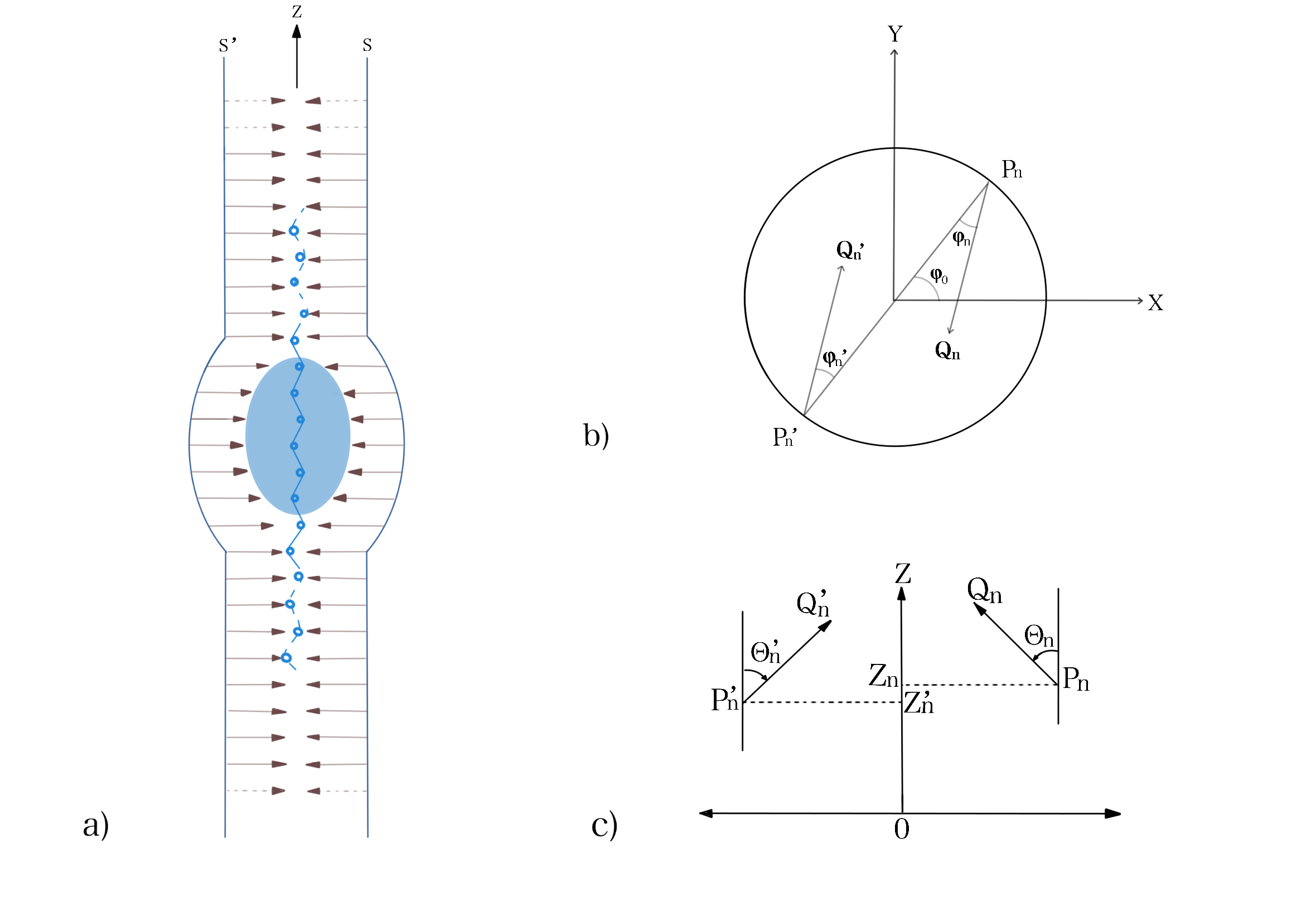
Consider the well-known B-form of DNA, where the sugar-phosphate backbone is represented by two ribbons, and , that spiral around each other along the -axis, as illustrated in Fig. 1a [30, 31]. The coordinates and represent the points where the -th and -th bases bases attached to their respective strands. These points are given by and , respectively, where with being the number of bases per turn in and . Here, is the radius of the circle, as shown in Fig. 1b. Additionally, and represent the angles of rotation of the -th base pair around the points and , respectively.
Below, we outline the general procedure for deriving the generalized Hamiltonian as an extension of the plane-base rotator model (for further details, see [33, 36]).
-
1.
The hydrogen bonds energy, or inter-strand energy, can be derived from the heuristic argument that it depends on the distance between the tip of the -th base and its complementary -th base base in the opposing strand, denoted as . For simplicity, we assume that the positions of the bases , , are identical, as shown in Fig. 1c.
-
2.
The quasi-spin operators , expressed in terms of the rotational angles and , with components
and, its complementary are introduced.
-
3.
An analogy is drawn between double-stranded DNA and an anisotropic coupled spin chain model to derive the intra-strand (or stacking) energy.
-
4.
The kinetic and potential energies of DNA and protein are added, where stands for the -th base displacement along the direction of the hydrogen bond, and denotes the displacement for -th peptide in the protein chain, with and as corresponding momenta.
-
5.
Finally, the coupling between the DNA with protein is introduced.
Considering all the listed above requirements, it is obtained the following Hamiltonian
| (1) | |||||
here, and are constants representing the stacking interaction energy between the -th base and its nearest neighbours in the two strands, and the hydrogen bond energy between the complementary bases, respectively. Additionally, and are elastic constants that characterize the behaviour of the hydrogen atom attached to the base and the amplitude of oscillations in the protein. The masses and correspond to the hydrogen atom attached to the base and the peptide in the protein, respectively. Finally, and are coupling coefficients that describe the interaction between thermal phonons and the DNA and protein, respectively
2.2 Weakly saturable approximation and cubic-quintic NLSE
We can exploit the fact that the Hamiltonian (1) is expressed in terms of quasi-spin operators, along with the generalized coherent states associated with the group. The average values of the quasi-spin operators, expressed in terms of their stereographic projections [55, 56, 57], are given by:
| (2) |
with and , where , and are related by
| (3) |
and their corresponding counterparts for the complementary strand. In addition, we consider the continuous limit
| (4) |
similarly, for , , and . This is possible because the length of excitations in DNA is much greater than the inter-site distance between neighbouring nucleotides. Therefore, by averaging the Hamiltonian (1) using the expressions in (2) and incorporating the above considerations, we obtain:
| (5) | |||||
Thus, the classical motion equations for , , where by symmetry of the double-stranded DNA , as well as for the displacements and , can be derived directly from (5) in a similar way. After reducing the system of coupled equations (for further details and references, see [36]), we obtain
| (6) |
here, we consider the parametric change , along with the condition that the parameter satisfy the strong inequality . Additionally, we define the following parameters
| (7) |
Expression (6) represents a generalized nonlinear Schrödinger equation with saturable nonlinearities, which fully describes the dynamics of the DNA-protein system. The analytical solutions of generalized nonlinear Schrödinger equations in saturable media present an intriguing challenge, and while some attempts have been made to solve the simplest versions of this equation directly [58, 59], a general solution remains elusive. In future work, we plan to explore the analytical solutions of Eq. (6). For the present study, however, we employ a weakly saturable approximation, where with . After performing the reparametrization , we obtain the cubic-quintic NLSE, which is given by
| (8) |
with parameters
| (9) |
In order to analyze the effects of the viscous medium on the system, we consider a simpler form of Eq. (8)
| (10) |
which was obtained by the following scale transformation
where and . Henceforth, we consider a reparametrizated form of Eq. (10), that is .
3 Perturbative analysis for the cubic-quintic NLSE solitons
3.1 The quasi-stationary method
The study of the perturbed cubic-quintic NLSE is crucial not only for understanding DNA-protein interactions but also for other branches of physics. In the previous analysis, the DNA-protein system was treated as an isolated system supporting the cubic-quintic NLSE. However, in reality, the DNA molecule interacts with its surrounding environment. Modeling the interaction between a single DNA molecule and its environment is a complex problem, but in a simplified scenario, it can be reduced to two primary effects: dissipation and the influence of the endogenous field [60]. For this analysis, we assume that the solvent consists of water molecules, which dampen the vibrations of the DNA bases, leading to the dissipation of nonlinear excitations in the system. To account for this, we introduce a perturbation term in Eq. (8) to study the evolution of the base-pair dynamics. To model the damping effects, we apply the multiple scales perturbation approach proposed by Y. Kodoma and M. J. Ablowitz, commonly known as the quasi-stationary method [61]. This method offers a significant advantage: it allows us to identify coherent, localized structures that emerge from the initial soliton-like solution. Before proceeding with the perturbative analysis of the molecular system, we first provide a brief overview of the quasi-stationary method.
Let us consider a perturbed nonlinear dispersive wave equation of the form
| (11) |
being and nonlinear functions of , . We are considering that the nonlinear equation (11) depends implicitly of , such as when we fix the parameter we obtain the unperturbed equation.
| (12) |
where is a solitary wave or a soliton solution. We write the solution now in terms of fast and slow variables:
| (13) |
It is denoted by the fast variables and by slow variables, and are parameters which depend on the slow variables. Here the variables satisfy , and and in order to remove secular terms. Therefore, these solutions are called quasi-stationary solutions . Thus, we assume an expression of the form
| (14) |
Substituting in the equation (11) we come up with the first order equations:
| (15) |
Here is a linearized equation of . We can denote by the solutions of the homogeneous adjoint problem satisfying
| (16) |
where is the adjoint operator to , we have
| (17) |
The last equation can be integrated to give the secularity conditions and, consequently, we will be in position to compute the solution for . by considering certain boundary conditions.
3.2 First order perturbation for the drop-soliton solution of the CQNSE
To implement the quasi-stationary method outlined above, we begin with the perturbed form of the cubic-quintic nonlinear Schrödinger equation (NLSE)
| (18) |
The right side of the equation (18) describes the damping effect caused by the viscous medium. The parameter is a coupling coefficient of the strength of viscous damping, which is very small at physiological temperatures. Taking the last assumption into account and in order to study the evolution of the nonlinear excitations in the DNA molecular chain we follow the perturbative analysis described on the previous section. When we obtain the unperturbed equation (10), which admits the following drop soliton-like solution [62]
| (19) |
with
| (20) |
Following the quasi-stationary method we write the soliton-like solution (19) in terms of fast and slow variables. Thus, we introduce a slow time variable , and , , , are functions of this time scale. We are able to write the envelope one soliton solution as
| (22) |
where
| (23) |
We assume an expression for
Neglecting higher order of , i.e., we focus on the first order soliton perturbation, such that
where
and , being and real functions. Substituting these expressions into the Eqs. (22) and (23), we obtain the following system
| (24a) | ||||
| (24b) | ||||
with
| (25a) | ||||
| (25b) | ||||
The operators and are self-adjoint and , . Consequently, the equations (24a) and (24b) have localized solutions around the drop soliton. The conditions of solvability of the system are given by the following secularity conditions
| (26a) | |||
| (26b) | |||
upon integrating the above expressions, we obtain
| (27) |
where is the energy of the soliton. In the presence of the perturbation term the parameters deform adiabatically, these adiabatic variations are given for (27). This is an easy way to corroborate the equations obtained by the Fredholm alternative. In order to find the perturbed soliton solutions we need to solve the homogeneous part of (24a) and (24b). Starting from (24a) and easily we can see that the solutions are:
| (28) |
| (29) | |||||
Using equation (28) and (29) and the secularity condition (27) we obtain the following solution
| (30) | |||||
with where and are arbitrary constants, with , , and defined as follows
Now, we solve the homogeneous part of equation (24b) obtaining
| (31a) | |||
| (31b) | |||
We construct the general solution as before, using the equations (31a) and (31b) and the variation of parameters. Thus, we have
| (32) | |||||
with . The expressions for , are given by
Now, let’s us consider in equation (19), which represents the center of the soliton and the center of the soliton phase, respectively, and from the secularity conditions (27). Thus, for (30) and (32), we have
| (33) |
Imposing the boundary conditions and we find the values for the arbitrary constants
Similar for (33) we obtain that
| (34) |
Imposing the boundary conditions and , we obtain
and
Finally, we can see that the general solution of the perturbed cubic-quintic NLSE is given by
| (35) |
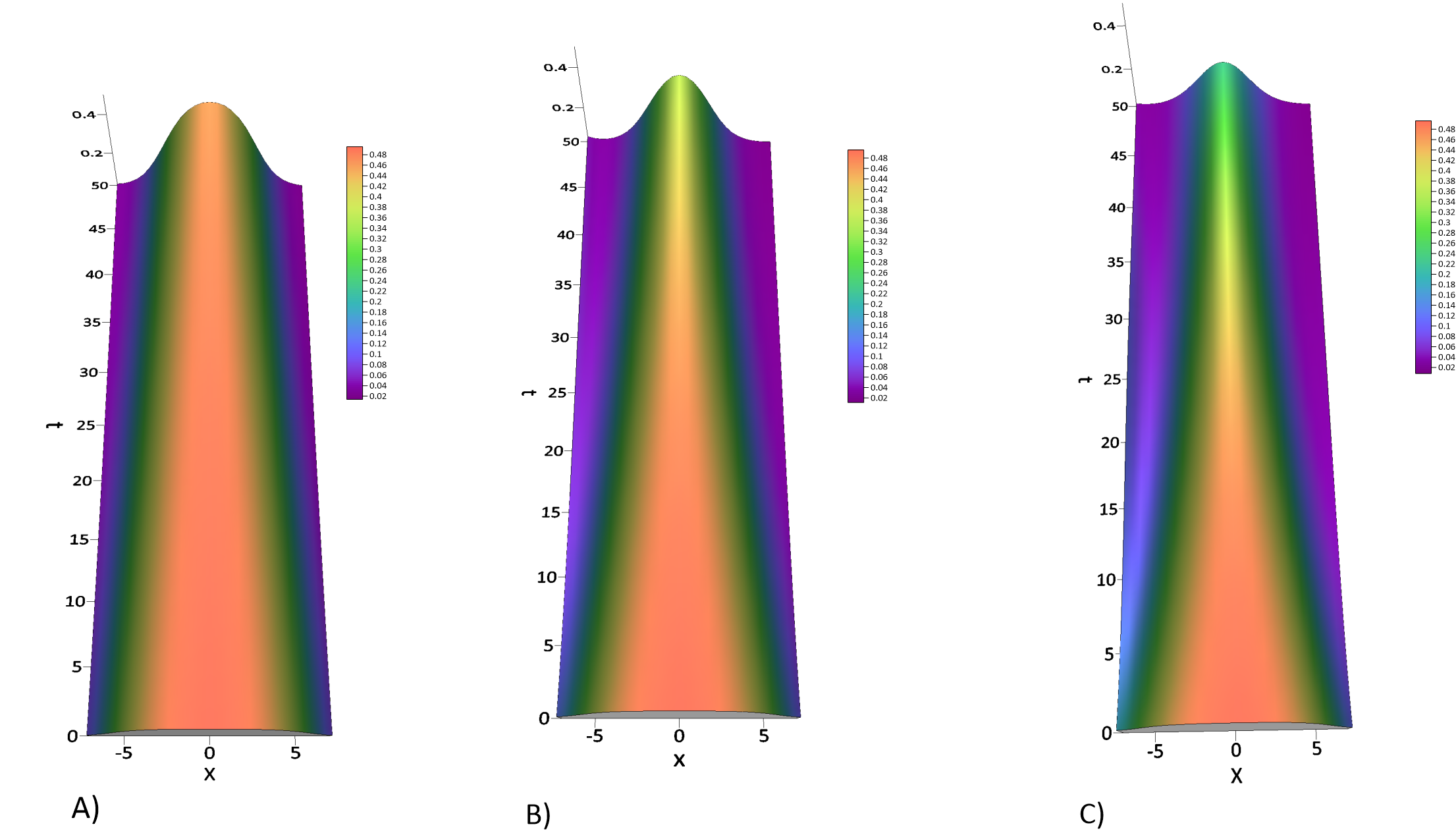
with and given by and (32). From the solution in Eq. (35), we can see that under perturbative effects, the drop soliton solution of Eq. (18) decays over time, as shown in Fig. 2. We can see from the solution (35) that under the perturbative effects the drop soliton solution of the equation (18) decay in time as shown in Fig. 2. For the case under consideration, is sufficiently small, returning us to the case of the perturbed NLSE [33]. We observe that the amplitude of the soliton decreases as time progresses, a consequence of the secularity conditions, while its velocity remains constant. Additionally, from the figures, we can note that the damping effect increases over a short period when the damping coefficient is larger. In general, the perturbed term in Eq. (18) can take the form of any function . For the specific case of DNA internal dynamics, we use to model the effect of a viscous medium. A similar approach is seen in the work by A. Biswas, where a different form of is considered for unchirped fibers in the context of the cubic-quintic NLSE [63].
4 Some comments on the transcription process of DNA transcription
The above analytical results can be applied to the transcription process, which is well-known for producing mRNAs that carry the genetic information necessary for protein synthesis. In addition to mRNA, transcription also generates transfer RNA (tRNA), ribosomal RNA (rRNA), and other RNA molecules that play crucial roles in cellular structure and catalysis. All of these RNA molecules are synthesized by RNA polymerase enzymes, which transcribe a DNA sequence into an RNA copy. The enzyme binds to the promoter region of the DNA and initiates transcription at a specific start site within the promoter. It continues synthesizing the RNA strand until it reaches a termination signal, at which point both the polymerase and the newly formed RNA molecule are released. Therefore, an RNA chain of 5000 nucleotides takes about 3 minutes to complete [64]. The DNA binds to the active site of the protein, causing the base pairs to separate and unwinding the DNA double helix. Recently, numerical studies have been made to understand the RNAp-DNA dynamics taking into account the helical coupling and the inhomogeneties of DNA [38, 39].

In this study, we neglect these contributions due to the fact that the contribution of inhomogeneities is small compared to homogeneous stacking. Besides, in these studies the localized inhomogeneity does not affect the bubble soliton sizes, even when the amplitude of inhomogeneity increases and the number of base pairs participating in the opening does not change due to this pattern of inhomogeneities. Moreover, we are interested in the analytic evolution of soliton-like solutions in the DNA-protein system under the viscous medium. From these numerical studies [38, 39] we obtained the approximate values of the hydrogen bonds coefficient () and the stacking energy costant(), the elastic constants () of the RNAp molecule and phonon chain ()) and their coupling coefficients to the DNA molecule ( and ), respectively. Also, the mass of the hydrogen atom attached to the base () and the mass of the peptide () are well-known.
Besides, it’s known that the cubic-quintic NLSE’s potential has several vacuum states, i.e, classical configurations with minimal energy. Therefore the solution of the equation of motion that lead to asymptotic values of have to coincide with minimum potentials. Thus, we can find the velocities of the displacement of the peptide and the hydrogen atom are given from:
without any loss of generality we can fix the value , it can be easily demonstrated that the solution properties can be represented in combinations of . Let us remind that for obtaining information on DNA properties we consider , and in our particular case the drop condition is whether . Thus, we can choose arbitrary and that satisfies this condition.
In previous studies, S. Sdravković and M. V. Satarić [60] found, using the Peyrard’s DNA model, the values of the speed and width of the soliton-like solution to be and , respectively, which means that 170 bases in each strand is covered by the soliton. The number of base pairs that participate in the opening process depends on the nature of the soliton. However, it is advantageous to have base pair opening with participation by fewer bases.
Finally, the value of the coupling coefficient of the strength of viscous damping depends on the physiological temperature (310 K). Thus, we have that is of the order of and the experimental value is .
5 Conclusion
In this study, we investigate the nonlinear dynamics of DNA and the evolution of nonlinear excitations induced by protein interactions and the surrounding viscous medium, using a quasi-stationary approach. Unlike previous studies that model DNA as a rigid molecular chain governed by the NLSE, we employ a cubic-quintic NLSE to account for the flexibility of the DNA strands and the physiological properties of the protein-DNA binding system. We do not consider helicoidal terms in our model, as numerical simulations using the Yakushevich model of DNA have shown that their impact on soliton-like solutions is minimal. The viscous medium introduces damping effects on the nonlinear excitations, leading to a reduction in the amplitude and a constant velocity of the drop-like soliton. This damping becomes more pronounced as the damping coefficient increases,causing the soliton to decay more rapidly over time. In the case of pure internal DNA dynamics, where , we can introduce various perturbations, such as periodic or pulse-like disturbances, depending on the nature of the double-stranded molecular system. These perturbations arise due to localized inhomogeneities in the DNA strands. In this work, we focus on the linear form of , but similar analyses can be applied to other types of localized perturbations, not just in DNA but also in any physical system governed by the cubic-quintic NLSE. One of the key advantages of the quasi-stationary approach is its versatility in analyzing different soliton-like solutions, such as kinks, breathers, drops, and bubbles. While this approach provides a useful approximation for understanding the behavior of DNA’s energy and information encoded in the strands, a discrete analysis would be required for a more in-depth understanding of the underlying complexities of the double-stranded DNA system.
Acknowledgments
OPT acknowledges CONAHCyT by a postdoctoral fellowship.
Data Availability Statement Data sharing not applicable to this article as no datasets were generated or analyzed during the current study.
References
- [1] Michel Peyrard, Nonlinear dynamics and statistical physics of DNA. Nonlinearity 17, R1–R40 (2004).
- [2] C. Bianca, M. Delitala, On the modelling of genetic mutations and immune system competition. Computers and Mathematics with Applications 61, 2362-2375 (2011).
- [3] Brown AJ, Mao P, Smerdon MJ, Wyrick JJ, Roberts SA, Nucleosome positions establish an extended mutation signature in melanoma. PLoS Genet 14 (11), e1007823 (2018).
- [4] Pich et al., Somatic and Germline Mutation Periodicity Follow the Orientation of the DNA Minor Groove around Nucleosomes. Cell 175, 1074–1087 (2018).
- [5] Benjamin Morledge-Hampton, John J. Wyrick, Mutperiod: Analysis of periodic mutation rates in nucleosomes. Computational and Structural Biotechnology Journal 19, 4177-4183 (2021).
- [6] Amar Singh and Navin Singh, Pulling short DNA molecules having defects on different locations. Phys. Rev. E 92, 032703 (2015).
- [7] Schumacher, B., Pothof, J., Vijg, J. et al, The central role of DNA damage in the ageing process. Nature 592, 695–703 (2021).
- [8] Chevizovich D, Michieletto D, Mvogo A, Zakiryanov F, Zdravković S, A review on nonlinear DNA physics. R. Soc. Open Sci. 7, 200774 (2020).
- [9] I.V. Likhachev, A. S. Shigaev, V.D. Lakhno, On the thermodynamics of DNA double strand in the Peyrard-Bishop-Dauxois model. Physics Letters A 510, 129547 (2024).
- [10] J. Brizar Okaly, Alain Mvogo, R. Laure Woulaché, T. Crépin Kofané, Nonlinear dynamics of DNA systems with inhomogeneity effects. Chinese Journal of Physics 56 (5), 2613-2626 (2018).
- [11] Christy Maria Joy, N. Ayyappam, N. Ayyappam, Dynamics of Peyrard Bishop model of DNA under the influence of solvent interaction. Materials Today: Proceedings 51, 1777–1781 (2022).
- [12] Nkeh Oma Nfor, Higher Order Periodic Base Pairs Opening in a Finite Stacking Enthalpy DNA Model. Journal of Modern Physics 12, 1843-1865 (2021).
- [13] Arnaud Djine, Nkeh Oma Nfor, Guy Roger Deffo, Serge Bruno Yamgoué, Higher order investigation on modulated waves in the Peyrard–Bishop–Dauxois DNA model. Chaos, Solitons & Fractals 181, 114706 (2024).
- [14] J. B. Okaly, A. Mvogo, C. B. Tabi, H. P. Ekobena Fouda, and T. C. Kofané, Base pair opening in a damped helicoidal Joyeux-Buyukdagli model of DNA in an external force field. Phys. Rev. E 102, 062402 (2020).
- [15] Muhammad Bilal Riaz, Marriam Fayyaz, Riaz Ur Rahman, Jan Martinovic, Osman Tunç, Analytical study of fractional DNA dynamics in the Peyrard-Bishop oscillator-chain model. Ain Shams Engineering Journal 15, 102864 (2024).
- [16] Kadiri Haritha and K V S Shiv Chaitanya, Statistical mechanics of DNA mutation using SUSY quantum mechanics. J. Phys. A: Math. Theor. 54, 305601 (15pp) (2021).
- [17] Franciele Polotto, Elso Drigo Filho, Jorge Chahine, Ronaldo Junio de Oliveira, Supersymmetric quantum mechanics method for the Fokker–Planck equation with applications to protein folding dynamics. Physica A 493, 286-300 (2018).
- [18] Song, D., Graham, T. and Loparo, J., A general approach to visualize protein binding and DNA conformation without protein labelling. Nat. Commun. 7, 10976 (2016).
- [19] Werner, M. H., Gronenborn, A. M. & Clore, G. M. Intercalation, DNA kinking, and the control of transcription. Science 271, 778–784 (1996).
- [20] Dickerson, R. E. DNA bending: The prevalence of kinkiness and the virtues of normality. Nucleic Acids Res. 26, 1906–1926 (1998).
- [21] Rudolf K. Allemann, Martin Egli. DNA recognition and bending. Chemistry & Biology. Volume 4, Issue 9, Pages 643-650 (1997).
- [22] Ludmila V. Yakushevich. Nonlinear Physics of DNA, 2nd Edition. Wiley‐VCH Verlag GmbH & Co. KGaA, Weinheim (2004).
- [23] Ijiro, K., and Mitomo, H., Metal nanoarchitecture fabrication using DNA as a biotemplate. Polym. J. 49 (12), 815–824 (2017).
- [24] Dey, S., Fan, C., Gothelf, K. V., Li, J., Lin, C., Liu, L., et al. DNA origami. Nat. Rev. Methods Prim. 1 (1), 13 (2021).
- [25] Laramy, C.R., O’Brien, M.N. & Mirkin, C.A, Crystal engineering with DNA. Nat. Rev. Mater 4, 201–224 (2019).
- [26] Ruixin Li, Mengxi Zheng, Anirudh S. Madhvacharyula, Yancheng Du, Chengde Mao, and Jong Hyun Choi, Mechanical deformation behaviors and structural properties of ligated DNA crystals. Biophysical Journal 121, 4078–4090, November 1 (2022).
- [27] Brandon Lu, Simon Vecchioni, Yoel P. Ohayon, James W. Canary, and Ruojie Sha, The wending rhombus: Self-assembling 3D DNA crystals. Biophysical Journal 121 (20), 4759–4765 (2022).
- [28] Huating Kong, Bo Sun, Feng Yu, Qisheng Wang , Kai Xia, Dawei Jiang . Exploring the Potential of Three-Dimensional DNA Crystals in Nanotechnology: Design, Optimization, and Applications. Adv Sci (Weinh). Aug; 10 (24):e2302021 (2023).
- [29] Lu, B., Simon, V., Ohayon, Y. P., Woloszyn, K., Markus, T., and Mao, C., Highly symmetric, self-assembling 3D DNA crystals with cubic and trigonal lattices. Small. 19, 3, 2205830 (2023).
- [30] S. Takeno, Shigeo Homma, Topological solitons and modulated structure of bases in DNA double helices, Prog. Theor. Phys. 70 (1), 308–311 (1983).
- [31] S. Takeno, Shigeo Homma, Coupled base rotator model for structure and dy- namics of DNA, Prog. Theor. Phys. 72 (4), 679–693 (1984).
- [32] M. Daniel, V. Vasumathi, Perturbed soliton excitations in the DNA double helix, Physica D, 231, 10-39 (2007).
- [33] V. Vasumathi, M. Daniel, Base-pairs opening and bubble transport in a DNA double helix induced by a protein molecule in a viscous medium, Physical Review E 80, 061904 (2009).
- [34] M. Daniel, M. Vanitha, Bubble solitons in an inhomogeneous, helical DNA molecular chain with flexible strands, Phys. Rev. E 84, 031928 (2011).
- [35] Slobodan Zdravkovic Miljko V. Sataric, and Muthiah Daniel, Kink solitons in DNA. International Journal of Modern Physics B 27:31 (2013).
- [36] M.A. Aguero, T.L. Belyaeva, V.N. Serkin, Compacton anti-compacton pair for hydrogen bonds and rotational waves in DNA dynamics, Commun. Nonlinear Sci. Numer. Simulat. 16, 3071–3080 (2011).
- [37] O. Pavón Torres, M. Aguero Granados, Exact traveling wave solutions in the coupled plane-base rotator model of DNA, International Journal of Non-Linear Mechanics 86, 8–14 (2016).
- [38] M. Saha, T.C. Kofané, DNA base pairs openings perturbed by the surrounding medium, Commun Nonlinear Sci Numer Simulat. 23, 1-9 (2015).
- [39] M. Saha, T.C. Kofané, Inhomogeneities and nonlinear dynamics of a helical DNA interacting with RNA-polymerase, Phys. Scr. 89, 085003 (2014).
- [40] G. Saccomandi, I. Sgura, The relevance of nonlinear stacking interactions in simple models of double-stranded DNA, J. R. Soc. Interface 3, 655-667 (2006).
- [41] H. Triki, T. R. Taha, Solitary wave solutions for a higher order nonlinear Schrödinger equation, Mathematics and Computers in Simulation 82, 1333–1340 (2012).
- [42] E. M. E. Zayed, Y. A. Amer, Many exact solutions for a higher order nonlinear Schrödinger equation with non-kerr terms describing the propagation of femtosecond optical pulses in nonlinear optical fibers, Computational Mathematics and Modeling, 28 (1), 118- 139 (2017).
- [43] A. D. D. Craik: Wave Interactions and Fluid Flows (Cambridge University Press, London, 1984).
- [44] O. E. Kurkina, A. A. Kurkin, T. Soomere, E. N. Pelinovsky, E. A. Rouvinskaya, Higher-order Korteweg-de Vries-like equation for interfacial waves in a symmetric three-layer fluid, Phys. Fluids 23, 116602 (2011).
- [45] A. Goullet, W. Choi, A numerical and experimental study on the nonlinear evolution of long-crested irregular waves, Phys. Fluids 23, 016601 (2011).
- [46] M. Gedalin, T. C. Scott, and Y. B. Band, Optical Solitary Waves in the Higher Order Nonlinear Schrödinger Equation, Phys. Rev. Lett. 78, 448 (1997).
- [47] V. G. Kartavenko, Soliton-like solutions in nuclear hydrodynamics, Sov. J. Nucl. Phys. 40, 240-246 (1984).
- [48] F. Kh. Abdullaev, A. Gammal, L. Tomio, T. Frederico, Stability of trapped Bose-Einstein condensates, Phys. Rev. A 63, 043604 (2001).
- [49] S. Burger, K. Bongs, S. Dettmer, W. Ertmer, and K. Sengstock, Dark Solitons in Bose-Einstein Condensates, Phys. Rev. Lett. 83, 5198 (1999).
- [50] C. Zhou and X. T. He, Stochastic diffusion of electrons in evolutive Langmuir fields, Phys. Scr. 50, 415 (1993).
- [51] I. Hacinliyan, S. Erbay, Coupled quintic nonlinear Schrödinger equations in a generalized elastic solid, J. Phys. A: Math. Gen. 37, 9387 (2004).
- [52] A. Kumar, S. N. Sarkar and A. K. Ghatak, Effect of fifth-order non-linearity in refractive index on Gaussian pulse propagation in lossy optical fibers, Opt. Lett. 11, 321-323, (1986).
- [53] O. Pavón-Torres, M. A. Agüero, T.L. Belyaeva, A. Ramirez, V. N. Serkin, Unusual self-spreading or self-compression of the cubic-quintic NLSE solitons owing to amplification or absorption, Optik 184, 446-456 (2019).
- [54] O. Pavón-Torres, M. A. Agüero-Granados, and R. Valencia-Torres. Adiabatic evolution of solitons embedded in lipid membranes. Phys. Scr. 99 125256 (2024).
- [55] A.M. Perelomov, Generalized coherent states and some of their applications, Sov. Phys. Usp. 20 (9) 703 (1977).
- [56] A.M. Perelomov, Generalized Coherent States and Their Applications, Springer, Verlag Berlin and Heidelberg GmbH and C. K, 2010.
- [57] O. Pavon Torres, M. Davila Davila, M. A. Aguero Granados, Introduction to coherent states approach for solving non-linear physical problems, Applied Physics Research, 8 (1), 106-124 (2016).
- [58] Nikolay A. Kudryashov. Bright and dark solitons in a nonlinear saturable medium. Physics Letters A 427, 127913 (2022).
- [59] Conrad Bertrand Tabi, Hippolyte Tagwo, and Timoléon Crépin Kofané. Modulational instability in nonlinear saturable media with competing nonlocal nonlinearity. Phys. Rev. E 106, 054201 (2022).
- [60] Zhravković S., Satarić M. V., The impact of viscosity on the DNA dynamics. Physica Scripta, Phys. Scr. 64 612 (2001).
- [61] Y. Kodoma, M. J. Ablowitz, Perturbations of solitons and solitary waves, Studies in applied mathematics 64, 225-245 (1981).
- [62] Vladimir N. Serkin, Tatyana L. Belyaeva, Igor V. Alexandrov, Gaston Melo Melchor, Novel topological quasi-soliton solutions for the nonlinear cubic-quintic Schrödinger equation, Proc. SPIE 4271, Optical Pulse and Beam Propagation III, 292-302 (2001).
- [63] A. Biswas, Quasi-stationary optical solitons with parabolic law nonlinearity, Optics Communications 216, 427-437 (2003).
- [64] B. Alberts, A. Johnson, J. Lewis, M. Raff, K. Roberts, and P. Walter, Molecular biology of the cell, 6th edition (2014).