Tube Loss: A Novel Approach for Prediction Interval Estimation and probabilistic forecasting

Abstract

This paper proposes a novel loss function, called ’Tube Loss’, for simultaneous estimation of bounds of a Prediction Interval (PI) in the regression setup, and also for generating probabilistic forecasts from time series data solving a single optimization problem. The PIs obtained by minimizing the empirical risk based on the Tube Loss are shown to be of better quality than the PIs obtained by the existing methods in the following sense. First, it yields intervals that attain the prespecified confidence level $t\in(0,1)$ asymptotically. A theoretical proof of this fact is given. Secondly, the user is allowed to move the interval up or down by controlling the value of a parameter. This helps the user to choose a PI capturing denser regions of the probability distribution of the response variable inside the interval, and thus, sharpening its width. This is shown to be especially useful when the conditional distribution of the response variable is skewed. Further, the Tube Loss based PI estimation method can trade-off between the coverage and the average width by solving a single optimization problem. It enables further reduction of the average width of PI through re-calibration. Also, unlike a few existing PI estimation methods the gradient descent (GD) method can be used for minimization of empirical risk. Finally, through extensive experimentation, we have shown the efficacy of the Tube Loss based PI estimation in kernel machines, neural networks and deep networks and also for probabilistic forecasting tasks. The codes of the experiments are available at https://github.com/ltpritamanand/Tube_loss

1 Introduction

In regression setting, machine learning (ML) algorithms predict the value of a variable $y$, often called dependent variable, given the value of an independent variable, say, $x$. Merely giving the predicted value of $y$ without attaching a measure of uncertainty with it, may not be useful in real world applications. Uncertainty quantification (UQ) is especially important, when the cost of incorrect prediction is high. For example, in planning replacement of a critical component of a nuclear reactor, failure of which may lead to a nuclear disaster, the information that the predicted value of its life is $2.5$ years without attaching a measure of uncertainty may not be useful. In contrast, if it is predicted that the life of critical component is between 2 and 3 years with, say, $99\%$ confidence, it throws out useful information. Such an interval, predicted for values of $y$, is often called a prediction interval (PI) with a pre-specified confidence (in this case $99\%$). Let us assume $(x_{i},y_{i}),i=1,2,...,m$, denote $m$ independent copies of the random variables $(x,y)$ having a joint distribution $p(x,y)$. With some abuse of notation, we denote by $(x,y)$, a pair of random variables as well as its values whenever the distinction is obvious.

A standard regression model provides an estimate of $\mathbb{E}(y|x)$ as the predicted value of $y$. However, for uncertainty quantification (UQ) of the output of a deep neural network (NN) in regression setting, researchers have obtained Prediction Interval (PI) of $y$ given $x$ with a given confidence (Khosravi et al. (2011b), Khosravi et al. (2011a), Nix & Weigend (1994), Pearce et al. (2018), Chung et al. (2021)). The limits of a PI are appropriately chosen quantiles of the distribution of NN outputs $y$ given $x$, and are thus, naturally, functions of $x$. Given $x$, let’s denote a PI of $y$ with confidence $t$ by $[\mu_{1}(x),\mu_{2}(x)]$ where $\mu_{1}(x)$ and $\mu_{2}(x)$ are the lower and the upper bounds of the interval, respectively, satisfying $P[\mu_{1}(x)<y<\mu_{2}(x)]=t$ where the probability is calculated based on the conditional distribution of $y$ given $x$.

Notice that, in the set-up described above, there are infinitely many choices of the bounds $\mu_{1}(x)$ and $\mu_{2}(x)$ satisfying the confidence constraint. Among all choices, the shortest PI, the PI having minimum average width $\mathbb{E}[\mu_{2}(x)-\mu_{1}(x)]$ is preferable, where the expectation is based on the marginal distribution of $x$. Suppose $[\hat{\mu}_{1}(x),\hat{\mu}_{2}(x)]$ denotes an estimate of PI $[\mu_{1}(x),\mu_{2}(x)]$ based on the data $(x_{i},y_{i}),i=1,2,...,m$, then we judge the quality of an estimated PI by two metrics. First, PI Coverage Probability (PICP) defined as the proportion of $y_{i}$s lying inside of the estimated interval. Naturally, we expect it to be close to $t$. Second, the Mean PI width (MPIW) defined as $\frac{1}{m}\sum_{i=1,..,m}[\hat{\mu}_{2}(x_{i})-\hat{\mu}_{1}(x_{i})]$. Among all intervals satisfying the constraint that PICP is greater than equal to $t$, the interval which minimizes MPIW is considered as the optimal choice of a PI. Following Pearce et al. (2018) we may call it High Quality (HQ) principle to be followed for choosing a PI.

For quantifying the uncertainty in regression task, various NN based PI estimation approaches have been proposed in the literature. Some, like the delta method (Hwang & Ding (1997),Chryssolouris et al. (1996)), the mean-variance estimation method (Nix & Weigend (1994)) and the Bayesian technique (MacKay (1992)) assume that the noises are independent Gaussian random variables. The PIs obtained by such methods may, thus, perform poorly, especially when the data distribution is highly skewed and/or heavy tailed. To get round this problem, some (Chung et al. (2021), Cui et al. (2020)) propose estimating $\mathbb{E}(y|x)$, and then the error distribution or its different moments. However, an alternative and a direct method for finding PI is to estimate appropriate quantiles of the conditional distribution of $y$ given $x$. The $q^{th}$ quantile of $y$ for a given $x$, say, $F_{q}(x)$ is defined as $P(y\leq F_{q}(x)|x)=q$, $q\in(0,1)$. Clearly, thus, an estimate of the interval $[F_{q}(x),F_{q+t}(x)]$ based on the training set $T$ provides a PI with confidence $t$ for all choices of $q$ satisfying $q,q+t\in(0,1)$. In other words, finding a PI with confidence $t$ simply requires the estimation of the quantile functions $F_{q}(x)$ and $F_{q+t}(x)$ for a $q$ satisfying $q,q+t\in(0,1)$. Notice that every choice of $q\in(0,1)$ such that $q+t\in(0,1)$ leads to a PI with confidence $t$. Thus, the method of construction of PI using quantiles subsumes the constraint on PICP.

In non-parametric framework, an estimate of $F_{q}(x)$, say, $\hat{F}_{q}(x)$ (Takeuchi et al. (2006)) is obtained by minimizing the empirical loss using pinball loss function which we discuss in detail in the next section. Thus, the resulting PI becomes $[\hat{F}_{q}(x),\hat{F}_{q+t}(x)]$. Notice that, for finding the lower and upper bounds of $[\hat{F}_{q}(x),\hat{F}_{q+t}(x)]$, the pinball loss minimization problem is to be solved independently for $q$ and $q+t$. Further, for finding a HQ PI, one needs to search for a $q$ among all feasible choices that minimizes the MPIW $\frac{1}{m}\sum_{i=1,..,m}[\hat{F}_{q+t}(x_{i})-\hat{F}_{q}(x_{i})]$. This amounts to solving two separate optimization problems repeatedly searching across all feasible choices of $q$. Consequently, PI estimation through this approach becomes computationally expensive. The question that naturally arises, whether the lower and upper bounds of a PI can be estimated simultaneously requiring solution of a single optimization problem.

Recently, in regression setting with Neural Network (NN), Khosravi et al. propose a solution to this problem by formulating Lower and Upper Bound Estimation (LUBE) Khosravi et al. (2011a) as a single constrained optimization problem. The LUBE searches for a PI as narrow as possible subject to the constraint of achieving the target confidence. The method uses a loss function which trades off between $(t-\textbf{PICP})_{+}$ and MPIW. However, for minimization of LUBE loss, gradient descent (GD) method cannot be used as it involves PICP, a step function, whose derivative is zero almost everywhere. This is inconvenient, considering GD as the standard method for training NN. Khosarvi et al. have used simulated annealing (SA), a non-gradient based optimization method, for training LUBE NN(Khosravi et al. (2011a)). Later, researchers use other non-gradient based training methods, like Genetic Algorithms (Ak et al., 2013), Gravitational Search Algorithms (Lian et al.,2016), PSO (Galvan et al., 2017, Wang et al., 2017), and Artificial Bee Colony Algorithms (Shen et al.,2018) for training the LUBE NN (Khosravi et al. (2011a)).

Considering the same setting and building on the same idea, Pearce et al. (2018) formulate estimation of PI as a constrained optimization problem similar to Khosravi et al. (2011). They replace the LUBE loss function by Quality-Driven (QD) distribution-free loss function, a loss function also trading-off between reducing the average width and attaining the target confidence. QD loss also involves the same step function as in LUBE. For enabling use of GD method in training NN they propose approximating this step function by a the product of two sigmoid functions. Unlike Khosravi et al. (2011) they incorporate the model uncertainty in PI estimation by ensembling models.

The above methods for simultaneous estimation of PI bounds are based on the HQ principle. However, these methods fail to attain the target confidence $t$. In contrast, the quantile-based PI estimation method is designed to attain the target confidence. However, estimation of the bounds $\hat{F}_{q}(x)$ and $\hat{F}_{q+t}(x)$ requires solving two different minimization problems. In this work, we introduce Tube Loss, a novel loss function, for the PI estimation and probabilistic forecasting task. The motivation behind introducing it is to yield estimates of the two quantile bounds simultaneously by solving a single optimization problem. In the following, we highlight our main contributions.

1. The minimizer of the empirical risk based on Tube loss is a pair of functions $(\hat{\mu}_{1}(x),\hat{\mu}_{2}(x))$ yielding the PI $[\hat{\mu}_{1}(x),\hat{\mu}_{2}(x)]$ which attains the target confidence $t$ asymptotically. We have provided a theoretical proof of this statement. This property makes it a natural choice for the loss function to be used in PI estimation and probabilistic forecasting.

2. For minimizing the average width of a PI with a prespecified confidence $t$, the PI needs to capture denser regions of the distributions of $y$ given $x$. To achieve it, we introduce an additional parameter $r$ in Tube loss function. By changing $r$, the PI bounds can be moved up or down simultaneously maintaining the coverage. Thus, a proper choice of $r$ enables capturing denser region of the $y$ values for each $x$. This is found to be very effective in reducing the width of the PI especially when the distribution of $y|x$ is skewed. For symmetric distribution, however $r=0.5$ is the default choice resulting in PI with symmetrically placed quantiles.

3. The proposed Tube loss function is differentiable almost everywhere (re Lebesgue measure) with non-zero gradients. It enables application of GD method for minimization of average Tube loss in different neural architectures. As discussed above, GD cannot be used for PI estimation using LUBE loss. Further, for enabling use of GD in PI estimation using QD loss, the step function in QD loss is approximated by a smooth function. The quality of PI, thus naturally depends on the quality of approximation as is evident from the experiments presented in Section 5. In contrast, during experimentation, GD method is used in Tube loss based learning models without encountering any problem.

4. The proposed estimation method allows trading off over-coverage for average width by introducing a user defined parameter $\delta$ in the optimization problem. The default choice of $\delta$ is zero. But, occasionally in some experiments we observe that the Tube loss-based PI achieves empirical coverage higher than the target $t$ on the validation set. In such cases, the average width of the PI on the test set can be further reduced by retraining the model (a process termed as re-calibration) with a smaller non zero value of $\delta$.

5. We have considered the Tube loss for PI estimation in kernel machines and neural networks in regression framework. A detailed derivation of the gradient descent algorithm for the Tube loss based kernel machines is given in Appendix B. Further, we have employed the Tube loss function into the different sequential deep learning architecture such as Long Short Term Memory (LSTM) Network (Hochreiter & Schmidhuber (1997)), Gated Recurrent Unit (GRU) (Chung et al. (2014)) and Temporal Convolutional Networks (TCN) (Lea et al. (2016)Lea et al. (2017)) for probabilistic forecasting task on time-series benchmark and wind datasets. The numerical results clearly show that the Tube loss based models result in PI of better quality compared to its existing alternatives.

The rest of the paper is organized as follows. In Section 2, we introduce some useful notations and mathematical preliminaries. Section 3 provides a brief survey of the literature for PI estimation. In Section 4, we deep dive into the properties of the tube loss function in detail. Section 5 presents experimental results on PI estimation comparing the tube loss with existing alternatives. In Section 6, we present the concluding discussion.

2 Notations & Mathematical Preliminaries

Let $\mathcal{X}$ and $\mathcal{Y}$ denote the domains of $x$ and $y$, respectively. In most applications $\mathcal{X}=\mathbb{R}^{n}$ and $\mathcal{Y}=\mathbb{R}$, where $\mathbb{R}$ is the set of real numbers. Let $T=\{(x_{i},y_{i}):x_{i}\in\mathcal{X},y_{i}\in\mathcal{Y},i=1,2,...,m\}$ be the training set, where $(x_{i},y_{i}),i=1,2,...,m$ are independently and identically distributed (iid) random variables having a joint distribution $p(x,y)$. With some abuse of notation, we denote by $(x,y)$, a pair of random variables as well as its values whenever the distinction is obvious.

In non-parametric framework, an estimate of $F_{q}(x)$, say, $\hat{F}_{q}(x)$ based on the training set $T$ is given by

$$\hat{F}_{q}(x)=\arg\min_{\mu}\sum_{i}\rho_{q}(y_{i}-\mu(x_{i})),$$ (1)

where, $\mu(.)$ belongs to a suitably chosen class of functions. And $\rho_{q}(u)$, the pinball loss function (Koenker & Bassett Jr (1978), Koenker & Hallock (2001)), is given by (Figure 1)

$$\rho_{q}(u)=\begin{cases}qu,~~~\mbox{ ~~~~~~~~if~~~~}u\geq 0,\\ (q-1)u,~~~\mbox{~otherwise}.\end{cases}$$ (2)

Figure 1: Pinball loss

Takeuchi et al. (2006) prove that for large $m$ if the conditional distribution of $y$ given $x$ does not contain any discrete component, the proportion of $y_{i}$’s below $\hat{F}_{q}(x)$ across all values of $x$ converges to $q$. Thus, for large $m$ and fixed $q$ such that $q+t\leq 1$, $[\hat{F}_{q}(x),\hat{F}_{q+t}(x)]$ provides a PI of $y$ with confidence $t$. However, for finding $\hat{F}_{q}(x)$ and $\hat{F}_{q+t}(x)$ one needs to solve the above optimization problem independently for $q$ and $q+t$. Further, for finding a HQ PI, among all feasible choices one needs to search for a $q$ such that the mean prediction interval width (MPIW) given by $m^{-1}\sum_{i}(\hat{F}_{q+t}(x_{i})-\hat{F}_{q}(x_{i}))$ is minimized. This amounts to solving two separate optimization problems repeatedly across feasible choices of $q$. Evidently, the PI estimation through this approach is computationally expensive.

Instead of estimating the bounds separately, simultaneous estimation of the lower and upper bounds of the PI (LUBE), say, $[\mu_{1}(x),\mu_{2}(x)]$ is first proposed by Khosravi et al. (2011a). They propose finding the estimates of $\mu_{1}(x)$ and $\mu_{2}(x)$ by minimizing the loss based on a novel loss function, say, LUBE. Building on the same idea as Khosravi et al. , Pearce et al. (2018) propose replacing LUBE by Quality Driven (QD) loss function citing some reasons for improvement.

Let $[\hat{\mu}_{1}(x),\hat{\mu}_{2}(x)]$ be the estimated PI on training set $(x_{i},y_{i})$, $i=1,2,..m$. Then, its empirical coverage (PICP), and mean width (MPIW) are defined as

$$PICP=m^{-1}\sum_{i=1,2,...,m}k_{i},$$ (3)

where,

$$k_{i}=\begin{cases}1,~\mbox{~if~~}y_{i}\in[\hat{\mu}_{1}(x),\hat{\mu}_{2}(x)],\\ 0,~\mbox{Otherwise,}\end{cases}$$ (4)

and

$$MPIW=m^{-1}\sum_{i=1,2,...,m}[\hat{\mu}_{2}(x_{i})-\hat{\mu}_{1}(x_{i})]],$$ (5)

respectively.

The LUBE and QD loss functions both involve PICP and MPIW. These loss functions are introduced for direct minimization of MPIW under the constraint that PICP is greater than equal to the target confidence $t$. In Section 3, we discuss in detail about these loss functions.

Unlike PI estimation using LUBE and QD losses, we in this paper take a different approach altogether. The idea is to find a sort of extension of pinball loss function, such that the minimization of the average loss based on it would yield the upper and lower bounds of PI simultaneously achieving the target confidence asymptotically. This loss function is differentiable almost everywhere (re Lebesgue measure), thus, enabling the application of GD for optimization. We call it Tube loss function. In Section 4 we present the Tube loss function in details.

3 A Brief Survey of The Literature

In this section, we summarize some recent and important work on PI estimation and probabilistic forecasting relevant to our work presented in this paper.

PI estimation in kernel machines :- In kernel machine literature a PI with confidence $t$ is given by $[\hat{F}_{q}(x),\hat{F}_{q+t}(x)]$ for fixed $0<q,q+t<1$ where, $\hat{F}_{q}(x)$ and $\hat{F}_{q+t}(x)$ are the $q^{th}$ and ${(q+t)}^{th}$ quantiles estimated independently. Specifically, for PI estimation in kernel machines presented in Section 5, we implement the quantile estimation method by Takeuchi et al. (2006). For estimation of $\tau^{th}$ quantile it requires the solution to the following optimization problem

$$\min_{(\alpha,\alpha_{0})}~[\frac{\lambda}{2}{\alpha}^{T}\alpha+\frac{1}{m}\sum_{i=1}^{m}\rho_{\tau}\big{(}y_{i}-\big{(}K(A^{T},x_{i})\alpha+\alpha_{0}\big{)}\big{)}]$$ (6)

where, $\rho_{\tau}(u)$ is as defined in (2), $K(A^{T},x)=\begin{bmatrix}k(x_{1},x),k(x_{2},x),..,k(x_{m},x)\end{bmatrix}$ and $k(x,y)$ is a positive semi-definite kernel (Mercer (1909)). Clearly, for the estimation of PI with confidence $t$, the problem (6) needs to be solved independently for $\tau=q$ and $\tau=q+t$, respectively. Further, to obtain a PI with minimum MPIW across different feasible choices of $q$ the independent estimation of ${F}_{q}(x)$ and ${F}_{q+t}(x)$ is to be repeated for a sufficiently large number of values of $q$.

PI estimation in Neural Networks:- The PI estimation problem in NN framework has been well studied. Some of the commonly used methods are the Delta Method Papadopoulos et al. (2001) Khosravi et al. (2011b), Bayesian Method Ungar et al. (1996) and Mean Variance Estimation (MVE) Method Nix & Weigend (1994). A systematic and detailed description of these methods can be found at Kabir et al. (2018). But, all these methods assume Gaussian noise distribution and thus, fail to ensure a consistent performance on a variety of data sets.

Khosravi et al. (2011) first propose a method for simultaneous estimation of lower and upper bounds of a PI in a distribution free setting by introducing a PI based loss function. This loss function is then used for training and development of NNs. They propose to minimize MPIW subject to the constraint that PICP is greater than equal to $t$ by introducing a novel loss function. Clearly this method is proposed on HQ principle. Let’s call this loss function as LUBE (Khosravi et al. (2011a)), and is given by,

$$LUBE=NMPIW\big{(}1+\gamma~(PICP)e^{-\eta(PICP-t)}\big{)},$$ (7)

where, $NMPIW(=\frac{MPIW}{R})$, $R(=max(y_{i})-min(y_{i}))$ is the range of response values $y_{i}$ and $\eta$ is a user-defined parameter can be used to magnify any small difference between $PICP$ and $t$, and $\gamma(PICP)=0,$ if $PICP\geq t$ and $1$, otherwise. This loss function as stated by Khosravi et al. (2011) is “nonlinear, complex and non differentiable." As a consequence, GD method cannot be applied for its minimization. They propose simulated annealing (SA), a non-gradient based method, for training NNs. Though SA was originally proposed as the training method, later various other non-gradient based methods are used for training the LUBE NN, including Genetic Algorithms (AK et al., 2013), Gravitational Search Algorithms (Lian et al. 2016), PSO (Galvan et al., 2017), and Artificial Bee Colony Algorithms (Shen et al, 2018).

LUBE has been extensively used by the researchers in various application-focused work, like energy load predictions (Pinson and Kariniotakis, 2013; Quan et al., 2014), wind speed forecasting (Wang et al., 2017, Ak et al.,2013), prediction of landslide displacement (Lian et al., 2016), gas flow (Sun et al., 2017) and solar energy (Galvan et al., 2017).

As discussed above, a major drawback of PI estimation using LUBE is, GD method cannot be used for its minimization. This is inconvenient considering that GD is now the standard method for training NNs. To overcome this problem, Pearce et al. (2018) building up on the same logic as (Khosravi et al. (2011a)), propose replacing CWC by QD loss function, which is given by

$$Loss_{QD}=MPIW_{capt.}+\lambda\frac{m}{t(1-t)}~max\big{(}0,(t-PICP)\big{)}^{2},$$ (8)

where $MPIW_{capt.}=\frac{\sum_{i=1}^{m}(\hat{\mu}_{2}(x_{i})-\hat{\mu}_{1}(x_{i})).k_{i}}{\sum_{i=1}^{m}k_{i}}$, $k_{i}$ is as defined in (4) and $\lambda$ is the user-defined trade-off parameter. Notice that in contrast to MPIW, $MPIW_{capt.}$ captures the average width for those points lying inside the PI. As explained in Section 3.3.1 of (Pearce et al. (2018)), like LUBE, $Loss_{QD}$ cannot be minimized directly using GD method since the derivative of the step function $PICP$ is zero almost everywhere. To remediate this and thus, enabling the use of GD method for minimization, they propose approximating the step function by the product of two sigmoid functions which has been used previously by Yan et al. (2004). They also propose using an ensemble of NN models instead of a single NN. The new model is found to yield PIs with shorter average widths.

It is worth mentioning here that both the loss functions LUBE and $Loss_{QD}$ are so constructed as to minimize the average width (MPIW or $MPIW_{capt.}$) of PI subject to the constraint that PICP is more than equal to the target coverage $t$. However, none of these methods guarantees PI to converge to the target coverage $t$ as the sample size becomes large, and allows for simultaneous movement of the lower and upper bounds to capture the denser parts of the data cloud leading to minimization of MPIW when the data distribution is skewed.

Probabilistic Forecasting in deep network:- Given the time-series data $\{y_{t},t=1,2,...,m\}$ on a variable $y$ over $m$ time points and a lag window $p\leq m$, the probabilistic forecasting of $y_{m+1}$ with coverage $t$ provides an interval $[\hat{y}_{m+1}^{q},\hat{y}_{m+1}^{q+t}]$ where, $\hat{y}_{m+1}^{q}$ and $\hat{y}_{m+1}^{q+t}$ are the estimates of $q^{th}$ and ${(t+q)}^{th}$ quantiles of the distribution $(y_{m+1}|y_{m},...,y_{m-p+1})$, $t+q\leq 1$. In the parametric framework, the joint distribution of $\{y_{t},t=1,2,...,m\}$ is assumed to be multivariate normal with some kind of dependence structure. Consequently, the conditional distribution of $(y_{m+1}|y_{m},...,y_{m-p+1})$ is normal with mean $\mu(y_{m},...,y_{m-p+1})$ and standard deviation $\sigma(y_{m},...,y_{m-p+1})$. The output layer of the deep network produces the maximum likelihood estimates of the mean and the standard deviation of the conditional distribution. Often, the normality assumption is based on mathematical convenience rather than evidence, which is often not adequate Gasthaus et al. (2019) for addressing the PI estimation problem. In the distribution-free setting, for obtaining probabilistic forecasts, the pinball loss based deep networks are used in different application contexts Zhang et al. (2018) Yu et al. (2021) Wang et al. (2019). These models require training of two independent deep networks for estimating the $q^{th}$ and $(t+q)^{th}$ quantiles using the pinball loss function Chen et al. (2020) Yang et al. (2002) Xu & Chen (2024). Our proposed method provides simultaneous estimation of the bounds leading to substantial saving in computational time.

4 Tube Loss function

In this section, first, we introduce the Tube loss function, a new class of loss functions, designed for the simultaneous estimation of the quantile bounds of PI. We then discuss its properties and also some important properties of the PI resulting from it.

For a given $t\in(0,1)$ and $u_{2}\leq u_{1}$, we define the Tube loss function as

$$\rho_{t}^{r}(u_{2},u_{1})=\begin{cases}tu_{2},~~~~~~~~~~~\mbox{if}~~~u_{2}>0,\\ -(1-t)u_{2},\mbox{~if}~u_{2}\leq 0,u_{1}\geq 0\mbox{~and~~}{ru_{2}+(1-r)u_{1}}\geq 0,\\ (1-t)u_{1},\mbox{~~~if}~u_{2}\leq 0,u_{1}\geq 0\mbox{~and~~}{ru_{2}+(1-r)u_{1}}<0,\\ -tu_{1},~~~~~~~~\mbox{if}~~u_{1}<0,\end{cases}$$ (9)

where $0<r<1$ is a user-defined parameter and ($u_{2}$, $u_{1}$) are errors, representing the deviations of $y$ values from the bounds of PI.

The Tube loss function is a kind of two-dimensional extension of Pinball loss function Koenker & Bassett Jr (1978). The plots of Tube loss are given for $r=0.5$ in Figure 2. For $r=0.5$, $\rho_{t}^{r}(u_{1},u_{2})$ is a continuous loss function of $u_{1}$ and $u_{2}$, and symmetrically located around the line $u_{1}+u_{2}=0$,$u\in\mathbb{R}$. In all experiments, where the noise distribution is assumed to be symmetric, the $r$ parameter in the Tube loss function should be $0.5$ to cover the denser region of $y$ values.

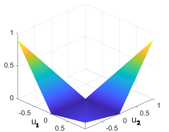
(a) t=0.9

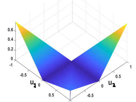
(b) t=0.8

Figure 2: Tube loss function

For sake of better intuition, if we consider $u_{1}=y-\mu_{1}$ and $u_{2}=y-\mu_{2}$, then, the Tube loss function reduces to

$$\rho_{t}^{r}(y,\mu_{1},\mu_{2})=\begin{cases}t(y-\mu_{2}),~~~~~~~~~~\mbox{~~if}~~y>\mu_{2}.\\ (1-t)(\mu_{2}-y),\mbox{~~~~if}~~~\mu_{1}\leq y\leq\mu_{2}\mbox{~and~~}y\geq{r\mu_{2}+(1-r)\mu_{1}},\\ (1-t)(y-\mu_{1}),\mbox{~~~~if}~~~\mu_{1}\leq y\leq\mu_{2}\mbox{~~and~~}y<{r\mu_{2}+(1-r)\mu_{1}},\\ t(\mu_{1}-y),~~~~~~~~~~~\mbox{if}~~~y<\mu_{1},\end{cases}$$ (10)

We have plotted the Tube loss function (10) in Figure 3 as a function of $y$, by fixing $\mu_{1}=-5$ and $\mu_{2}=5$. It clearly shows that the Tube loss function is a kind of juxtaposition of two Pinball loss functions.

(a) t=0.95

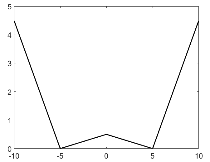
(b) t=0.90

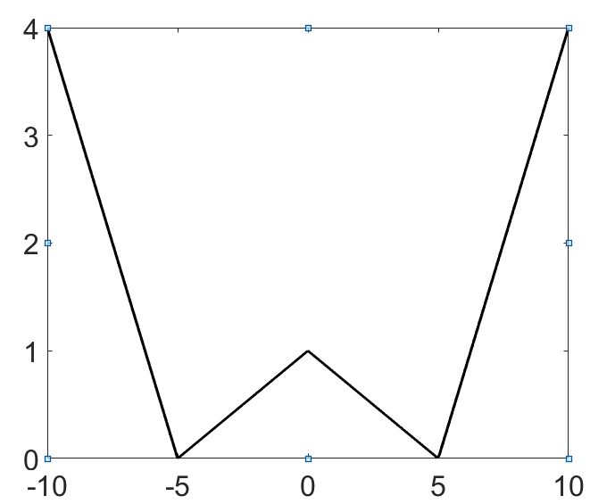
(c) t=0.80

Figure 3: Tube Loss with $\mu_{1}=-5$ and $\mu_{2}=5$.

For given $(x_{i},y_{i})$, $i=1,2,..m$, and a confidence $t\in(0,1)$, the estimation of PI $[\hat{\mu}_{1}(x),\hat{\mu}_{2}(x)]$ with tube loss function is given by

$$[\hat{\mu}_{1}(x),\hat{\mu}_{2}(x)]=\arg\min_{\mu_{1},\mu_{2}}\sum_{i=1}^{m}\rho_{t}^{r}(y_{i},\mu_{1}(x_{i}),\mu_{2}(x_{i})),$$

where, $\mu_{1}(.)$ and $\mu_{2}(.)$ belong to a suitably chosen class of functions and $\rho_{t}^{r}(y,\mu_{1}(x),\mu_{2}(x)$, is given by

$$\rho_{t}^{r}(y,\mu_{1}(x),\mu_{2}(x))=\begin{cases}t(y-\mu_{2}(x)),~~~~~~~~~~\mbox{~~if}~~y>\mu_{2}(x).\\ (1-t)(\mu_{2}(x)-y),\mbox{~~~~if}~~~\mu_{1}(x)\leq y\leq\mu_{2}(x)\mbox{~and~~}y\geq{r\mu_{2}(x)+(1-r)\mu_{1}(x)},\\ (1-t)(y-\mu_{1}(x)),\mbox{~~~~if}~~~\mu_{1}(x)\leq y\leq\mu_{2}(x)\mbox{~~and~~}y<{r\mu_{2}(x)+(1-r)\mu_{1}(x)},\\ t(\mu_{1}(x)-y),~~~~~~~~~~~\mbox{if}~~~y<\mu_{1}(x),\end{cases}$$ (11)

By controlling the value of the user parameter $0<r<1$, the upper and the lower bounds of the PI could be moved up and down simultaneously. This is a consequence of Proposition 2 to be discussed in detail in Sub-section 4.2. From Figures 6 (cf. Section 5), it is evident that with increase in the value of $r$ the upper and the lower bounds of PI move up simultaneously. As stated above, an appropriate choice of $r$ may, thus, help in reducing MPIW by capturing denser regions of data cloud, especially when the conditional distributions of $y$ given $x$ across different values of $x$ are skewed.

Unlike the PI based loss functions discussed above, Tube loss has two unique features which ensure the generation of high quality PIs. The results of our experiments presented in Section 5 clearly bear it out. First, the coverage, measured by PICP, achieves the pre-fixed confidence approximately. This is a consequence of Proposition 1 (iii) stated below. In simple language it states that PICP converges to the pre-fixed confidence asymptotically i.e., as the size of the training set tends to infinity. Thus, the PIs are automatically calibrated in an asymptotic sense. We provide a theoretical proof of it. Second, a hyper parameter $r$ that we introduce in the loss function provides the flexibility of moving the PI bounds up and down simultaneously. Thus, by properly adjusting the value of $r$ we may be able to capture the denser parts of the data cloud inside the interval. It may lead to substantial reduction of MPIW. This is a consequence of the results proved in Proposition 1 (i)-(ii). For data generated by a symmetric distribution like Gaussian, the default choice $r=0.5$ produces HQ PIs, but for data generated by asymmetric distributions, by choosing an appropriate value of $r$ a substantial reduction of MPIW may be achieved. The experimental results reported in Section 5.1 clearly borne out this fact. The PI for $r=0.5$ yields a HQ interval when the noises are generated by a symmetric (Gaussian) distribution, on the other hand, for noises generated by an asymmetric (Chi-squared) distribution, the choice $r=0.1$ seems to be appropriate.

4.1 Asymptotic properties of the Tube loss function

In this section, we prove that given a training set $T=\{(x_{1},y_{1}),....,(x_{m},y_{m}):x_{i}\in\mathbb{R}^{n},y_{i}\in\mathbb{R}\}$, and $t\in(0,1)$, the PI $[{\mu}^{*}_{1}(x),{\mu}^{*}_{2}(x)]$ obtained by minimizing the empirical risk $\frac{1}{m}$ $\sum_{i=1}^{m}L_{t}^{r}(y_{i},\mu_{1}(x_{i}),\mu_{2}(x_{i}))$ asymptotically achieves the target coverage $t$. In other words, for a sufficiently large training set, the coverage of the PI achieves the target coverage approximately. The proof follows the reasoning outlined by Takeuchi et al. (2009), who established it for the pinball loss.

First, we prove a lemma assuming an independently and identically distributed (iid) random variables set up. Let $\{y_{1},y_{2},....,y_{m}\}\subset\mathbb{R}$ are iid following the distribution of a continuous random variable $Y$ and $t\in(0,1)$. Let us define the following subsets of $\mathbb{R}$: $\Re_{1}(\mu_{1},\mu_{2})=\{y:y>\mu_{2}\}$, $\Re_{2}(\mu_{1},\mu_{2})=\{y:\mu_{1}<y<\mu_{2},y>r\mu_{2}+(1-r)\mu_{1}\}$, $\Re_{3}(\mu_{1},\mu_{2})=\{y:\mu_{1}<y<\mu_{2},y<r\mu_{2}+(1-r)\mu_{1}\}$ and $\Re_{4}(\mu_{1},\mu_{2})=\{y:y<\mu_{1}\}$. Notice that the sets $\Re_{i}(\mu_{1},\mu_{2}),i=1,2,3,4$ are so defined that they do not include the points on the boundaries. Suppose $({\mu}^{*}_{1},{\mu}^{*}_{2})$ is the minimizer of $\frac{1}{m}$$\sum_{i=1}^{m}L_{t}^{r}(y_{i},\mu_{1},\mu_{2})$ with respect to $(\mu_{1},\mu_{2})$, and $m_{k}$ denotes the number of data points in $\Re_{k}({\mu}^{*}_{1},{\mu}^{*}_{2})$ . Then we have the following lemma.

Lemma. As $m\rightarrow\infty$, with probability $1$ the following results hold:

(i) $\frac{m_{1}}{m_{2}}\rightarrow\frac{1-t}{t}$, (ii) $\frac{m_{4}}{m_{3}}\rightarrow\frac{1-t}{t}$, and (iii) $\frac{m_{1}+m_{4}}{m_{2}+m_{3}}\rightarrow\frac{1-t}{t}$.

Proof:- The proof is provided at the Appendix A.

We now extend the above lemma to the regression setup introduced at the outset of this section. As stated above the problem is to minimize the empirical risk $\frac{1}{m}$ $\sum_{i=1}^{m}L_{t}^{r}(y_{i},\mu_{1}(x_{i}),\mu_{2}(x_{i}))$ with respect to $(\mu_{1}(x),\mu_{2}(x))$ where $\mu_{1}(x)$ and $\mu_{2}(x)$ belong to an appropriately chosen class of functions . With some of abuse of notations we let $m_{k}$ to denote the cardinality of the set $\Re_{k}({\mu}^{*}_{1}(x),{\mu}^{*}_{2}(x))$ $(k=1,2,3,4$) inducing a partition of the feature space (as shown in Figure 4), where $({\mu}^{*}_{1}(x),{\mu}^{*}_{2}(x))$ is the minimizer of the empirical risk $\frac{1}{m}$ $\sum_{i=1}^{m}L_{t}^{r}(y_{i},\mu_{1}(x_{i}),\mu_{2}(x_{i}))$. We then have the following proposition.

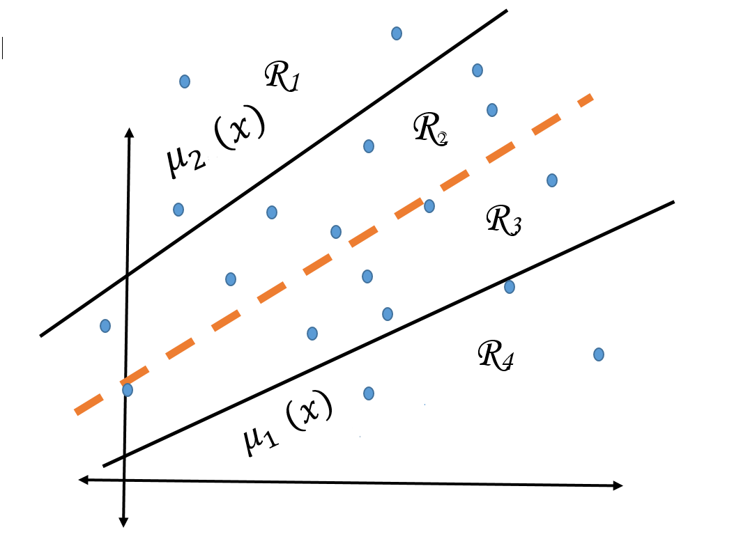
Figure 4: PI tube loss, red line represents the convex combination of ${\mu}^{*}_{1}(x)$ and ${\mu}^{*}_{2}(x)$, i,e., $r{\mu}^{*}_{1}(x)+(1-r){\mu}^{*}_{2}(x)$, $0<r<1$. Blue dots represent data points $(x_{i},y_{i})$, $i=1,2,,..,m$.

Proposition 1. For $t\in(0,1)$ as $m\rightarrow\infty$ the following results hold with probability $1$,
(i) $\frac{m_{1}}{m_{2}}\rightarrow\frac{1-t}{t}$, (ii) $\frac{m_{4}}{m_{3}}\rightarrow\frac{1-t}{t}$ (iii) $\frac{m_{1}+m_{4}}{m_{2}+m_{3}}\rightarrow\frac{1-t}{t}$

provided $(x_{i},y_{i}),i=1,2,...,m$ are iid following a distribution $p(x,y)$ with $p(y|x)$ continuous and the expectation of the modulus of absolute continuity of its density satisfies $\lim_{\delta\to 0}E[\epsilon(\delta)]=0$.

Proof: The proof follows from the the proof of the Lemma above and Lemma 3 of Takeuchi et al. (2006).

4.2 The $r$ parameter and movement of the PI bounds

The Proposition 2 clearly entails that the coverage of the PI obtained by minimizing the proposed tube loss achieves the target confidence asymptotically. Here, we show by choosing $r$ appropriately how the PI tube can be moved up and down.

Let us suppose that $(\hat{\mu}_{1}^{r_{2}}(x),\hat{\mu}_{2}^{r_{2}}(x))$ is the minimizer of the average loss for $r=r_{2}$ i,e. $\frac{1}{m}$ $\sum_{i=1}^{m}L_{t}^{r_{2}}(y_{i},\mu_{1}(x_{i}),\mu_{2}(x_{i}))$. Also we assume that there are $m_{k}^{r_{2}}$ points in the set $\Re_{k}(\hat{\mu}_{1}^{r_{2}}(x),\hat{\mu}_{2}^{r_{2}}(x)),(k=1,2,3,4$). Similarly, for $r_{1}(<r_{2})$, we assume $(\hat{\mu}_{1}^{r_{1}},\hat{\mu}_{2}^{r_{1}})$ is the minimizer of the average loss for $r=r_{1}$, and there are $m_{k}^{r_{1}}$ points in the set $\Re_{k}(\hat{\mu}_{1}^{r_{1}}(x),\hat{\mu}_{2}^{r_{1}}(x)),(k=1,2,3,4$). Now, Proposition 1 (iii) entails that asymptotically $t$ fraction of $y$ values should lie inside each of the PIs $[\hat{\mu}_{1}^{r_{1}},\hat{\mu}_{2}^{r_{1}}]$ and $[\hat{\mu}_{1}^{r_{2}},\hat{\mu}_{2}^{r_{2}}]$. But, since $r_{1}<r_{2}$, the $\frac{m_{2}^{r_{1}}}{m_{3}^{r_{1}}}>\frac{m_{2}^{r_{2}}}{m_{3}^{r_{2}}}$, which implies $\frac{m_{1}^{r_{1}}}{m_{4}^{r_{1}}}>\frac{m_{1}^{r_{2}}}{m_{4}^{r_{2}}}$ for large $m$, by using the (i) and (i) of Preposition 1. In other words, changing $r$ from $r_{1}$ to $r_{2}$ moves the tube down. Thus, the PI bounds can be moved up and down by changing $r$.

As stated above, by controlling $r$ MPIW can be reduced. But, the Tube loss function $\rho_{t}^{r}(u_{1},u_{2})$ is discontinuous at the separating plane $\{(u_{1},u_{2}):ru_{2}+(1-r)u_{1}=0\}$ when $r\neq 0.5$. It is worth mentioning here, that the experimental results presented in Section 5 are obtained by the application of GD method. The discontinuity has not caused any problem. The gradient descent algorithm for Tube loss based kernel machines is derived and detailed at the Appendix B.

4.3 Re-calibration

Often, it is observed that the coverage of the PI obtained by training the model on a small training data may be significantly greater than the target confidence $t$ on the validation set. In such cases, re-calibration of the model by trading off MPIW with the average loss in the training set may lead to a PI with smaller MPIW in the test set. The optimization problem with user defined parameter $\delta>0$ is then formulated as follows:

$$\min_{(\mu_{1},\mu_{2})}[\sum_{i=1}^{m}\rho_{t}^{r}(y_{i}-\mu_{1}(x_{i}),y_{i}-\mu_{2}(x_{i}))+\delta\sum\limits_{i=1}^{m}|(\mu_{2}(x_{i})-\mu_{1}(x_{i})|].$$ (12)

4.4 Comparative Analysis of loss functions used for PI Estimation

In Table 1, we list the desirable criteria of an ideal PI method. Based on these criteria, we then compare the Quantile, LUBE, QD and Tube loss based PI estimation methods. The LUBE and QD loss-based methods provide direct PI estimation but fail to satisfy a few important criteria, such as asymptotic coverage guarantee and PI movement to capture the denser regions of $y$ values. While quantile-based PI estimation method satisfies some of these criteria but it fails to estimate the upper and lower bounds simultaneously and also, does not support re-calibration. Tube loss-based PI methods, on the other hand, provide simultaneous estimation of the quantile bounds, an opportunity to minimize the average width of PI using re-calibration and moving PI tube up and down while retaining the asymptotic guarantee of coverage. However, none of the PI model ensures the individual calibration (Chung et al. (2021)), which requires that PI should cover $t$ fraction of $y$ values for each given $x$.

	Quantile	LUBE	QD loss	Tube loss
Asymptotic guarantees	$\checkmark$	$\times$	$\times$	$\checkmark$
Direct PI estimation	$\times$	$\checkmark$	$\checkmark$	$\checkmark$
PI tube movement	$\checkmark$	$\times$	$\times$	$\checkmark$
Continious loss function	$\checkmark$	$\times$	$\times$	$\checkmark$
Gradient descent solution	$\checkmark$	$\times$	$\checkmark$	$\checkmark$
Re-calibration	$\times$	$\checkmark$	$\checkmark$	$\checkmark$
Individual Calibration	$\times$	$\times$	$\times$	$\times$

Table 1: Comparisons of the Quantile , LUBE, QD loss and Tube loss based PI estimation models

5 Experimental Results

We present here the results of the experiments that we have run to compare the performances of PI based on Tube loss function with that of PIs based on the standard loss functions. We consider PI estimation in kernel machines, NN and probabilistic forecasting. We train different PI estimation methods and assess their performances on test set $\{(x_{i},y_{i}):i=1,2,..,k\}$, using the following evaluation metrics.

1. Prediction Interval Coverage Probability (PICP): The fraction of $y_{i}$ values in the test set lying inside of estimated PI.

2. Mean Prediction Interval Width (MPIW): The average width of the estimated PI across different values of test $x_{i}$.

As stated at the outset, HQ principle requires a PI to minimize MPIW subject to the constraint that PICP is greater than equal to the nominal confidence level $t$. In the following, for comparing two PI estimation methods, say, A and B we follow this rule: A is better than B (i) if $PICP(A)\geq t$ and $PICP(B)<t$, or (ii) $min\{PICP(A),PICP(B)\}\geq t$ and $MPIW(A)<MPIW(B)$. Further, in experiments where the data are generated synthetically from a known distribution, the true quantiles of $y$ given $x$ are known for all values of $x$, and hence the true PI. In such cases, to get a better insight about their performances, we may compare the $PICP$ and $MPIW$ of the estimated PIs with that of the true PI locally in different regions of $x$. Also, to measure the deviation between the estimated PI, say, $[\hat{\mu}_{1}(x),\hat{\mu}_{2}(x)]$ and the true PI, say, $[\mu_{1}(x),\mu_{2}(x)]$, we consider the Sum of Mean Square of Error (SMSE) given by $\frac{1}{k}\sum_{i=1}^{k}(\hat{\mu}_{1}(x_{i})-\mu_{1}(x_{i}))^{2}+\frac{1}{k}\sum_{i=1}^{k}(\hat{\mu}_{2}(x_{i})-\mu_{2}(x_{i}))^{2}$.

5.1 Tube loss in kernel machine:-

Let us generate two synthetic datasets, say, A and B, of the form $\{(x_{i},y_{i}),i=1,2,..,1500\}$, where $x_{i}$ is generated from uniform distribution between $0$ and $1$ ($U(0,1)$) and $y_{i}$, using the relation

$$y_{i}=\frac{sinx_{i}}{x_{i}}+\epsilon_{i},$$ (13)

where, $\epsilon_{i}$ is a random noise. For dataset A, $\epsilon_{i}$ is generated from $\mathcal{N}(0,0.8)$, a symmetric distribution, and for data set B from $\chi^{2}(3)$, a positively skewed distribution. We train the model using 500 data points and the rest we use for testing. For estimation of linear PI tube, we use linear kernel. For the estimation of the non-linear PI tube, we use RBF kernel of the form $k(x_{1},x_{2})=e^{-\gamma||(x_{1}-x_{2})||^{2}}$, where $\gamma$ is the parameter.

For dataset A, we obtain PIs with nominal confidence levels $t=0.8$ and $t=0.9$ using Tube loss function with $r=0.5$ and $\delta=0$. The PICP and the MPIW of the resulting PI in the test data set corresponding to $t=0.8$ ($t=0.9$) are found to be $0.799$ ($0.909$) and $2.10$ ($2.78$), respectively. Figure (5) shows the estimated PI on test set with target $t=0.8$ and $t=0.9$.

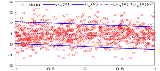
(a)

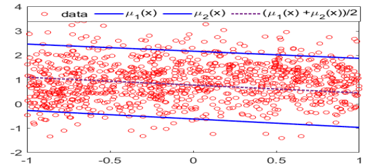
(b)

Figure 5: Tube loss based SVPI estimation for (a)$t=0.8$ and (b) $t=0.8$.

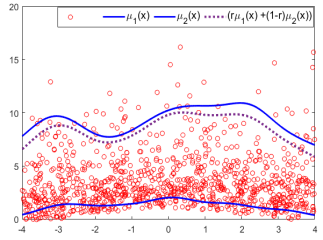
(a) r= 0.8

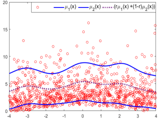
(b) r = 0.5

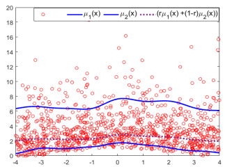
(c) r= 0.3

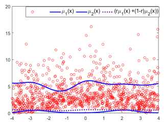
(d) r= 0.1

Figure 6: Location of PI tube changes with r values in Tube loss based kernel machine.

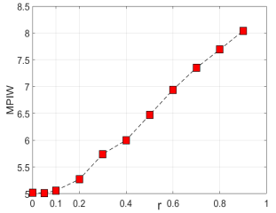
(a)

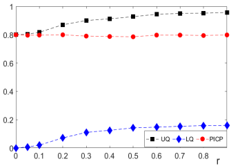
(b)

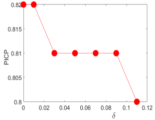
(c)

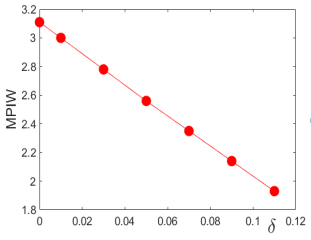
(d)

Figure 7: Plot of (a) r against MPIW ,(b) PCIP, UQ and LQ for dataset B. Plot of (c) $\delta$ against PICP ,(d) $\delta$ against MPIW on Servo dataset.

For dataset B, we target to estimate the PI for $t=0.8$ with RBF kernel. In Figure 6 (b), the Tube loss based kernel machine with parameters $r=0.5$ and $\delta=0$ obtains the PICP $0.79$ and MPIW $6.47$. However, the estimated PI tube does not capture the densest region of response values leading to large MPIW values as noise in the data is from the asymmetric $\chi^{2}$ distribution. For this, we need to shift the estimated PI tube downwards. Figure 6 (a) (c) and (d) shows the PI obtained by the tube loss-based kernel machine for $r=0.8,0.3,$ and $0.1$. As we decrease the $r$ values, the estimated PI tube moves downward, capturing denser regions of $y$ values with lower MPIW. We have plotted the MPIW, PICP, LQ, and UQ obtained by the tube loss-based kernel machine against different $r$ values in Figure 7 (a) and (b). The LQ (Lower Quantile) and UQ (Upper Quantile) are the fractions of $y_{i}$ lying below the upper and lower bound functions of our estimated PI tube. The LQ and UQ values decrease with the decrease in $r$ values leading to a downward movement of the PI tube with lesser MPIW values without compromising the PICP of estimate. The MPIW improves significantly with the decrease in $r$ values. In fact, MPIW values improve by $21.80\%$, if we decrease the $r$ from $0.5$ to $0.1$.

It is worth mentioning here, for data set A where the noises are generated by a symmetric distribution, the default choice $r=0.5$ leads to HQ PI. On the other hand, for the data set B, noise distribution is positively skewed, the lower value of $r$ yields the HQ PI.

	Model	(q+t,q)/(r,$\delta$)	PICP	MPIW	Time (s)
A	Q Ker M	(0.95,0.15)	$0.78\pm 0.017$	$2.088\pm 0.109$	219.38
	Q Ker M	(0.90,0.10)	$0.78\pm 0.019$	$2.002\pm 0.068$	221.72
	Q Ker M	(0.85,0.05)	$0.79\pm 0.025$	$2.151\pm 0.078$	217.38
	T Ker M	(0.6,0)	$0.80\pm 0.012$	$2.165\pm 0.068$	56.93
	T Ker M	(0.5,0)	$0.80\pm 0.018$	$2.156\pm 0.069$	61.50
B	Q Ker M	(0.90,30)	$0.59\pm 0.032$	$4.6609\pm 0.153$	138.05
	Q Kerl M	(0.95,0.35)	$0.58\pm 0.023$	$5.5369\pm 0.272$	146.60
	Q Ker M	(0.80,20)	$0.59\pm 0.027$	$3.6196\pm 0.143$	146.41
	T Ker M	(0.3,0)	$0.60\pm 0.032$	$3.495\pm 0.168$	39.07
	T Ker M	(0.2,0)	$0.601\pm 0.028$	$3.174\pm 0.165$	41.55

Table 2: Quantile based Kernel Machine (Q ker M) and Tube loss based kernel Machine (T ker M) on dataset A and B. Q kernel M involves parameters (q+t,q) and T kernel M involves (r, $\delta$).

Finally, for both datasets, we compare the performances of PIs using quantile based estimation method and Tube loss based estimation method in kernel machines by replicating each experiment $10$ times to capture the sampling variation in PICP and MPIW. For dataset A (B), we run these experiments for nominal confidence level $t=0.8$ ($t=0.6$). Notice that for quantile based estimation, the choice of parameter $q$ and for Tube loss based estimation, the choice of parameters $r$ and $\delta$ are crucial for generating HQ interval. We have considered a few choices. The results of our experiments are presented in Table 1. Following the rule stated at the outset for comparison of PI estimation methods, it is evident that for data set A, Tube loss based method outperforms quantile based method. The PICPs of PIs obtained by Quantile kernel Machine for all three choices of $q$ fail to attain the nominal confidence level $0.8$. Other notable advantage of the Tube loss based kernel machine is the significant improvement in the training time. Further, as expected for symmetric noises, the Tube loss with $(r=0,\delta=0)$ yields HQ PIs.

For data set B, the results are similar. Clearly, the Tube loss based kernel machine improves training time of the Quantile based kernel machine significantly. It also obtains the nominal confidence level $0.6$, while the Quantile kernel machine fails to attain the same. Further, by choosing $r$ suitably in Tube loss kernel machine, the MPIW could be reduced substantially. This is expected given that the noises are generated from a positively skewed distribution, and thus, moving the bounds downward leads to substantial reduction of MPIW.

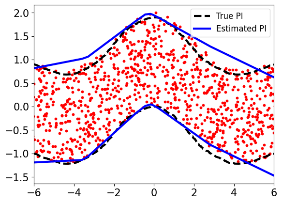
(a) QD loss based NN

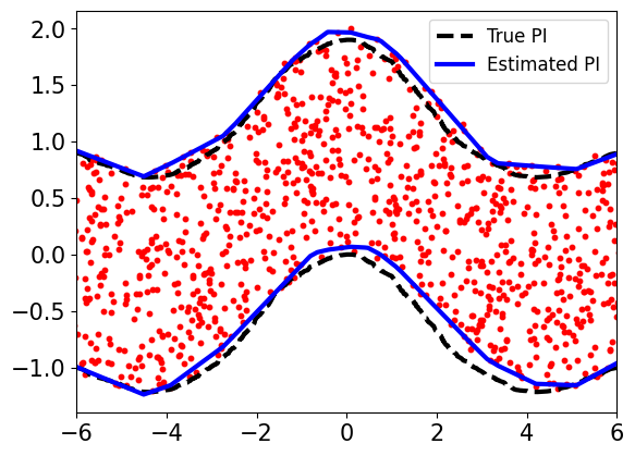
(b) Tube loss based NN

Figure 8: Comparison of Tube loss and QD loss function based NNs

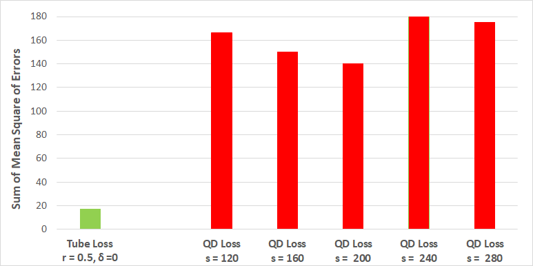
Figure 9: Tube loss based NN approximates true PI better than QD loss.

Re-calibration effect of parameter $\delta$:- The parameter $\delta$ in the Tube loss based kernel machine is practically useful for improving the MPIW on the test set. To show this, we have considered the popular Servo (167 $\times$ 5) Karl Ulrich (2016) dataset and separated the $10\%$ of data points as a testing set. The remaining data points were trained with a 10-fold cross-validation method for target $t=0.80$ PI with $r=0.5$ and $\delta=0$. The mean PICP reported on the validation set was $0.82$. Since the observed PICP was significantly larger than the target PICP on the validation set, therefore, there was a scope to obtain lesser MPIW on the test set by increasing the value of $\delta$. We have increased the value of $\delta$ till the observed PICP on the validation set decreases to the target $t=0.8$, shown in Figure 7 (c). It causes about 44$\%$ improvement in test MPIW as shown in Figure 7 (d) while maintaining the required coverage. However, this facility remains missing in the quantile based kernel machine.

5.2 Tube Loss in Neural Network

In the NN framework Pearce et al. (2018) show that the PI obtained by QD loss performs slightly better than that obtained by LUBE Khosravi et al. (2011a) in terms of PICP and MPIW producing smoother and tighter boundaries. This improvement is attributed to the use of GD method for optimization of QD loss instead of Particle Swarm Optimization (PSO) Kennedy & Eberhart (1995), a non-gradient based method, used for LUBE loss. Also they compare PI with QD loss with the PI obtained by Mean Variance Estimation (MVE) method, Nix & Weigend (1994). They observe that QD method performs better than the MVE method when the noises are generated from a skewed distribution, specifically from an $exp(1/x^{2})$. It is worth mentioning here that for noises generated from a skewed distribution, the Tube loss based PIs outperform the quantile based PIs (cf. Section 5.1).

Here, we perform a simple experiment to show how the Tube loss based PI outperforms the QD based PI in terms of SMSE, a local measure of smoothness and tightness introduced at the outset of Section 5. For this, we generate $1000$ data points $(x_{i},y_{i})$ using the equation,

$$y_{i}=\frac{sin(x_{i})}{x_{i}}+\epsilon_{i},$$ (14)

where $x_{i}$ is $U(-2\pi,2\pi)$ and $\epsilon_{i}$ is from $U(-1,1)$.

We train the tube Loss-based NN model and the QD loss-based NN model to obtain a PI with nominal confidence level 0.95. After tuning, we fix the NN model, containing 100 neurons in the hidden layer with ’RELU’ activation function and two neurons in the output layer. ’Adam’ optimizer was used for training the NNs. Figure 8 (a) shows the PI obtained by the QD loss and Figure 8 (b) the Tube loss with $r=0.5$ (Figure 8 b) along with the true PI. Clearly the PI generated by the Tube loss is smoother and tighter compared to that generated by the QD loss. The true PI is computed by obtaining $97.5\%$ and $2.5\%$ quantiles of the conditional distribution of $y|x$ for different values of $x$.

The observed (PICP, MPIW) for Tube loss and QD loss are $(0.95,1.78)$ and $(0.98,2.17)$, respectively. For QD loss, the tuning of the soften parameter $s$ is important but, is a tedious task. We tune parameters $s$ and $\lambda$ of QD loss to arrive at the choice $s=200$ and $\lambda=0.1$. We then compute the SMSEs of the PIs. Figure 9 presents the SMSE comparison of tube loss with QD loss for different values of softening parameter $s$. Evidently, the performance of the QD loss based PI is sensitive to the choice of $s$, and thus, on the quality of approximation of the step function by the sigmoidal functions.

Benchmark Datasets

Here, we consider six open-access data sets considered by Pearce et al. (2018) and others (Hernandez-Lobato & Adams, 2015;Gal and Ghahramani, 2015; Lakshminarayanan et al., 2017) for recent work on uncertainty estimation in deep learning. Pearce et al. (2018) compare the performance of QD-Ens, a QD loss based PI using five NNs per ensemble, with that of MVE-Ens in terms of PICP and MPIW. The NN models are asked to output $95\%$ PI. For three data sets (Boston, Concrete and Wine) QD-Ens PIs fail to attain the nominal confidence level. Although, the results reported in their paper suggest that for all six data sets the QD-Ens PIs perform better than the MVE-Ens PIs. Following the same experimental setting as considered by Pearce et al. (2018) we obtain the PIs using Tube loss function. For the Tube loss based NN model, $r$, $\delta$, learning rate, decay rate and batch size are tuned. Adam optimizer is used in both Tube loss and QD loss based NN models. More tuning and experimental details are provided at the Appendix C. The experimental results are presented in Table 2. Clearly, for all six data sets Tube loss based PIs attain nominal confidence level $0.95$ and performs better than the QD loss function.

Clearly, Tube loss based PIs outperform QD-Ens based PIs. Some of the reasons are: Tube loss avoids approximations for enabling the use of GD method, asymptotically guarantees nominal confidence level and facilitates movement of the PI bounds by adjusting the tuning parameter $r$.

Dataset	PICP		MPIW		Better
	$QD-Ens$	$Tube_{loss}$	$QD-Ens$	$Tube_{loss}$
Boston	0.92 + 0.01	0.95 $\pm$ 0.01	1.16 $\pm$ 0.02	1.12 $\pm$ 0.04	$\surd$
kin8NM	0.96 $\pm$ 0.00	0.95 $\pm$ 0.00	1.25 $\pm$ 0.01	1.10 $\pm$ 0.01	$\surd$
Energy	0.97 $\pm$ 0.01	0.95 $\pm$ 0.03	0.47$\pm$ 0.01	0.36 $\pm$ 0.05	$\surd$
Concrete	0.94 $\pm$ 0.01	0.95 $\pm$ 0.02	1.09$\pm$ 0.01	1.22 $\pm$ 0.06	$\surd$
Naval	0.98 $\pm$ 0.00	0.95 $\pm$ 0.01	0.28$\pm$ 0.01	0.24 $\pm$ 0.03	$\surd$
Wine	0.92 $\pm$ 0.01	0.95 $\pm$ 0.01	2.33$\pm$ 0.02	2.80 $\pm$ 0.08	$\surd$

Table 3: PI quality metric on real-world benchmark datasets.

5.3 Tube loss for probabilistic forecasting with deep networks

We now assess the performance of the Tube loss function for probabilistic forecasting tasks using different deep network forecasting architectures.

At first, we consider the six popular benchmark time-series data sets viz., Electric (BP & Ember. (2016)), Sunspots (SIDC & Quandl. ), SWH (NDBC ),Temperature (machinelearningmastery.com ), Female Birth (datamarket.com ) and Beer Production (Australian (1996)). For probabilistic forecasts we use Long Short Term Memory (LSTM) Network (Hochreiter & Schmidhuber (1997)). We compare the probabilistic forecasts of the Tube loss based LSTM (T-LSTM) with that of the Quantile based LSTM (Q-LSTM) for these datasets. We use $70\%$ of the data points for training and rest for testing. Out of the training sets, $10\%$ of the observations are used for validation.

Dataset	PICP		MPIW		Training Time (SEC)		Improvement	Improvement
	Q-LSTM	T- LSTM	Q-LSTM	T-LSTM	Q-LSTM	T-LSTM	in Time(s)	in MPIW	Better
Electric	0.95	0.95	18.23	17.02	145	58	60 $\%$	6.60 $\%$	$\surd$
Sunspots	0.93	0.95	121.09	113.98	839	442	47 $\%$	5.87 $\%$	$\surd$
SWH	0.96	0.96	0.52	0.35	5119	2733	46 $\%$	32.69$\%$	$\surd$
Temperature	0.95	0.94	24.82	15.56	1135	447	60 $\%$	37.30$\%$
Female Birth	0.95	0.96	28.20	28.09	118	43	63 $\%$	0.40$\%$	$\surd$
Beer Production	0.94	0.95	134.8	42.91	132.8	89.6	33 $\%$	68.17$\%$	$\surd$

Table 4: Comparison of Quantile based LSTM (Q-LSTM) and Tube loss based LSTM (T-LSTM) on real-world time-series datasets

Since these datasets are being used by other researchers, for each dataset, we tune and fix LSTM hidden layer structure, drop out layer and window size based on information available in the literature. We then obtain the PI using the Tube loss function, and also using quantiles. The nominal confidence level considered is $0.95$. In Table 4, the PICP, MPIW and training time in seconds are reported for Q-LSTM and T-LSTM. Clearly, the T-LSTM based PIs outperform Q-LSTM based PIs in five out of 6 datasets. Also re-calibration of T-LSTM (cf. (16)) based forecasts leads to furtrher reduction of MPIW. The main advantage of T-LSTM over Q-LSTM is significant improvement in MPIW values and training time. As stated above, Q-LSTM needs to be trained twice whereas T-LSTM requires only once.

The probabilistic forecasts for each of the data sets considered in Table 3 are presented in Figure 5. The details of the LSTM architectures, and the values of the tuning parameters used for obtaining the probabilistic forecasts for each data set are presented in Table 4.

Dataset (Size)	LSTM Structure	Batch Size		Up,Low	r,$\delta$	Window Size	Learning Rate
		Q- LSTM	T-LSTM	Q- LSTM	T-LSTM		Q-LSTM	T-LSTM
Sunspots (3265)	[256(0.3) ,128(0.2)]	128	128	0.98,0.03	0.5,0	16	0.001	0.001
Electric Production (397)	[64]	32	16	0.98,0.03	0.5,0.01	12	0.01	0.001
Daily Female Birth (365)	[100]	64	128	0.98,0.03	0.5,0.01	12	0.01	0.005
SWH (2170)	[128(0.4),64(0.3),32(0.2)]	300	300	0.98, 0.03	0.5, 0.01	100	0.001	0.001
Temperature (3651)	[16,8]	300	300	0.98, 0.03	0.5, 0.01	100	0.001	0.0001
Beer Production (464)	[64,32]	64	64	0.98, 0.03	0.1, 0.01	12	0.001	0.0001

Table 5: Tuned parameter values for Q-LSTM and T-LSTM model for considered benchmark datasets. The LSTM architecture [128(0.4),64(0.3),32(0.2)] means that three hidden layers with neurons 128, 64 and 32 respectively and each hidden layer is followed by a drop out layer which are 0.4,0.3 and 0.2 respectively.

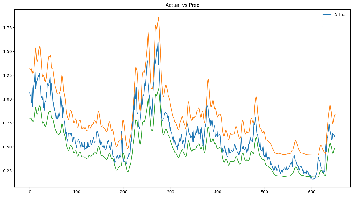
(a) SWH

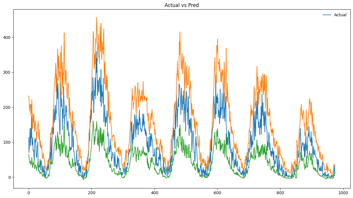
(b) Sunspot

(c) Electric Production

(d) Beer Production

Figure 10: Probabilistic forecast of LSTM with proposed Tube loss function.

Dataset	PICP		MPIW		Improvement
	$QD^{+}$-LSTM	T- LSTM	$QD^{+}$-LSTM	T-LSTM	in MPIW	Better
Electric	0.96	0.95	54.63	17.02	68.84 $\%$	$\surd$
Sunspots	0.43	0.95	24.06	113.98	NA	$\surd$
SWH	0.96	0.96	0.36	0.35	2.78$\%$	$\surd$
Female Birth	0.94	0.96	38.98	28.09	27.94$\%$	$\surd$
Temperature	0.79	0.95	5.94	15.56	73.13 $\%$	$\surd$
Beer Production	0.96	0.95	159.71	42.91	NA	$\surd$

Table 6: Comparison of Extended Quality Driven loss based LSTM (QD⁺ LSTM) and Tube loss based LSTM (T-LSTM) on real-world time-series datasets

In a distribution-free setting, quantile-based deep learning models are the most popular choice for probabilistic forecasting. However, for comparison purposes, we also evaluated the performance of deep learning models trained with the QD loss function for probabilistic forecasting. A significant practical challenge in training deep learning models with the QD loss function is the frequent occurrence of NaN losses during computation. But, the extended Quality Driven (QD⁺) loss function (Salem et al. (2020)) solves this problem up to some extent. Consequently, we have implemented the QD⁺ loss function based deep forecasting models for obtaining the probabilistic forecast.

We tune the parameter values of QD+ loss function based LSTM well and compare its performance with the Tube loss based LSTM model on time-series benchmark dataset at Table 6. Unlike, the Quantile and Tube loss based LSTM models, the QD+ loss function based LSTM model fails to obtain the consistent performance. Out of six datasets, it fails to obtain the target coverage on three datasets. In case of Sunspots and Temperature datasets, the QD⁺ loss function based LSTM obtains very poor performance.

5.3.1 Probabilistic forecasting of wind speed

For further validity of the Tube loss function, We need to evaluate its performance with other commonly used deep neural architectures for forecasting such as LSTM, GRU and TCN.

Probabilistic forecasting of wind speed is crucial for effective decision-making in the wind power industry. We use the Tube loss function into the LSTM, Gated Recurrent Unit (GRU) and Temporal Convolution Network (TCN) model for wind speed probabilistic forecasting. We have compared the Tube loss based deep forecasting models with the quantile based deep forecasting models. We have also used the QD⁺ loss function (Salem et al. (2020)) in deep probabilistic forecasting of wind speed for the comparisons.

Model	Loss/Method	PICP	MPIW	Time (s)
LSTM	Tube	0.9511	3.159	229.61
LSTM	QD+	0.9682	3.886	212.17
LSTM	Quantile	0.9899	5.443	258.66
GRU	Tube	0.9550	3.288	148.36
GRU	QD+	0.9658	3.951	97.63
GRU	Quantile	0.9821	5.302	299.25
TCN	Tube	0.9550	3.371	32.69
TCN	QD+	0.9829	4.43	46.24
TCN	Quantile	0.9806	4.738	165.94

Table 7: Performance of deep forecasting models on the Jaisalmer Dataset

Dataset:- We have acquired a time series dataset of hourly wind speed measurements at 120m height obtained from Jaisalmer through the National Renewable Energy Laboratory website at https://developer.nrel.gov/docs/wind/wind-toolkit/ https://developer.nrel.gov. The first $75\%$ hourly wind-speed observation was taken as training set and thereafter next $15\%$ of observations was taken as validation set. The last $15\%$ of observations was used for testing.

Table 7 compares the Tube loss based LSTM, GRU and TCN models with QD++ loss function and quantile based deep forecasting models on the the Jaisalmer wind datasets. We can observe that the Tube loss based deep forecasting models obtain the better performance than the QD+ loss and quantile based deep forecasting models. Also quantile based deep forecasting models are computationally expensive than the Tube loss. Figure 11 shows the probabilistic forecasting of the Tube loss based LSTM model on Jaisalmer dataset.

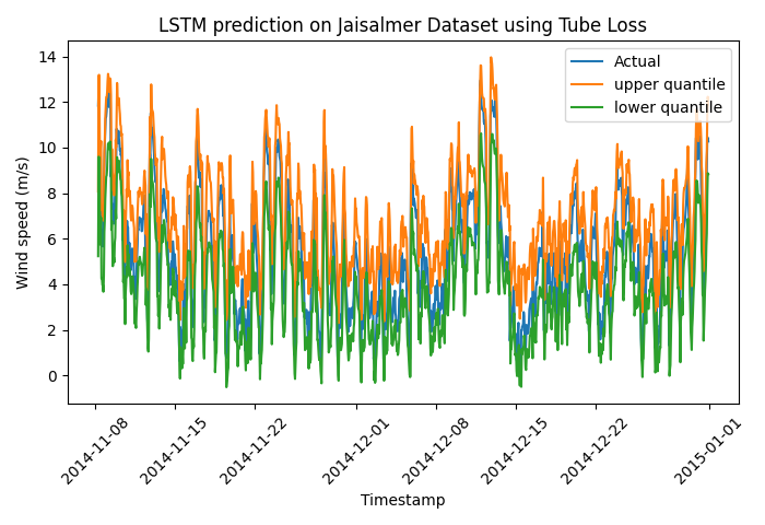
(a)

Figure 11: Probabilistic forecast of the Tube loss based LSTM on Jaisalmer wind dataset.

6 Future Work

The Tube loss function does not only offer a convenient way for PI estimation and probabilistic forecasting but, also opens a set of promising research directions. The future work requires a thorough theoretical analysis of the Tube loss function, similar to the analysis of the pinball loss function available in the literature. The Tube loss function asymptomatically guarantees to attain the target confidence $t$, thus, for small sample sizes it may not attain the target confidence $t$. A potential future direction is to refine Tube loss-based networks by applying techniques from the literature, such as group batching (Chung et al. (2021)), or introducing orthogonality constraints (Feldman et al. (2021)) to improve the local calibration. The other important research direction may be to use the Tube loss function for conformal regression and then compares its performances with the existing conformal regression techniques.

In most applications related to the text processing, the target variable is multidimensional. An interesting proble is to consider extension of the proposed PI estimation methodology for multidimensional target variable. Also, it would be interesting to apply the proposed methodology for probabilistic forecasting considering various neural architectures used in different domains of applications, such as solar irradiance, cryptocurrency prices, exchange rates, stock prices, ocean wave heights, pollution rates, and weather forecasting to name a few.

Appendix A Appendix A

Proof of the Lemma:

Let us assume that $\#\{y_{i}|y_{i}=\mu_{2}^{*}\}=k_{1}$, $\#\{y_{i}|y_{i}=r\mu_{2}^{*}+(1-r)\mu_{1}^{*}\}=k_{2}$, and $\#\{y_{i}|y_{i}=\mu_{1}^{*}\}=k_{3}$, where $\#$ represents the cardinality of a set. In other words, $k_{1},k_{2}$ and $k_{3}$ represent the number of points on the boundary sets. Thus, we obtain $m_{1}+k_{1}+m_{2}+k_{2}+m_{3}+k_{3}+m_{4}=m$.

Let us choose, $\delta_{1}^{*}\in[0,\epsilon_{1})$, $\delta_{2}^{*}\in[0,\epsilon_{2})$, where $\epsilon_{1}$ and $\epsilon_{2}$ are positive real numbers, such that $\epsilon_{1}$ < $\min\limits_{y_{i}<\mu_{1}^{*}}(|\mu_{1}^{*}-y_{i}|)$, $\epsilon_{2}$ < $\min\limits_{y_{i}>\mu_{2}^{*}}|(y_{i}-\mu_{2}^{*})|$, and $r\epsilon_{2}+(1-r)\epsilon_{1}<\min\limits_{\mu_{1}^{*}<y_{i}<\mu_{2}^{*}}|y_{i}-(r\mu_{2}^{*}+(1-r)\mu_{1}^{*})|$, which entails

$$\#\{y_{i}:\mu_{2}^{*}<y_{i}\leq\mu_{2}^{*}+\delta_{2}^{*}\}=0,~~\#\{y_{i}:\mu_{2}^{*}<y_{i}\leq\mu_{2}^{*}-\delta_{2}^{*}\}=0,~~\#\{y_{i}:\mu_{1}^{*}<y_{i}\leq\mu_{1}^{*}+\delta_{1}^{*}\}=0,$$

$$\#\{y_{i}:\mu_{1}^{*}<y_{i}\leq\mu_{1}^{*}-\delta_{1}^{*}\}=0,~~\#\{r\mu_{2}^{*}+(1-r)\mu_{1}^{*}<y_{i}\leq r(\mu_{2}^{*}+\delta_{2}^{*})+(1-r)(\mu_{1}^{*}+\delta_{1}^{*})\}=0,$$

$$\hskip-569.05511pt\#\{r\mu_{2}^{*}+(1-r)\mu_{1}^{*}<y_{i}\leq r(\mu_{2}^{*}-\delta_{2}^{*})+(1-r)(\mu_{1}^{*}-\delta_{1}^{*})\}=0.$$

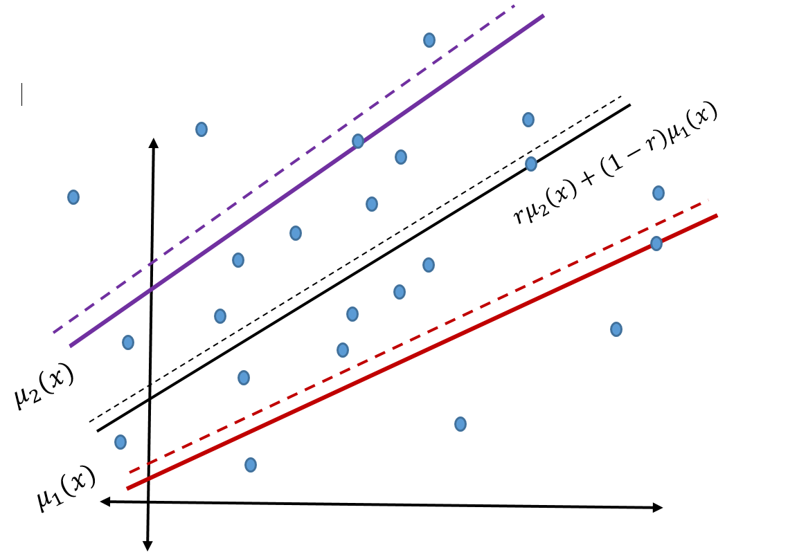
Figure 12:

Given that $(\mu_{1}^{*},\mu_{2}^{*})$ is an optimal solution, we have $\sum_{i=1}^{m}L_{t}^{r}(y_{i},\mu_{1}^{*}+\delta_{1}^{*},\mu_{2}^{*}+\delta_{2}^{*})-\sum_{i=1}^{m}L_{t}^{r}(y_{i},\mu_{1}^{*},\mu_{2}^{*})\geq 0$. We now evaluate the difference of the sums for each of the following ten sets inducing a partition of $\mathbb{R}$.

$R_{1}=\{y_{i}:y_{i}>\mu_{2}^{*}+\delta_{2}^{*}\}$, $R_{2}=\{y_{i}:\mu_{2}^{*}<y_{i}\leq\mu_{2}^{*}+\delta_{2}^{*}\}$, $R_{3}=\{y_{i}:y_{i}=\mu_{2}^{*}\}$,
$R_{4}=\{y_{i}:r(\mu_{2}^{*}+\delta_{2}^{*})+(1-r)(\mu_{1}^{*}+\delta_{1}^{*})<y_{i}<\mu_{2}^{*}\}$, $R_{5}=\{y_{i}:r\mu_{2}^{*}+(1-r)\mu_{1}^{*}<y_{i}\leq r(\mu_{2}^{*}+\delta_{2}^{*})+(1-r)(\mu_{1}^{*}+\delta_{1}^{*})\}$, $R_{6}=\{y_{i}:y_{i}=r\mu_{2}^{*}+(1-r)\mu_{1}^{*}\}$, $R_{7}=\{y_{i}:\mu_{1}^{*}+\delta_{1}^{*}<y_{i}<r\mu_{2}^{*}+(1-r)\mu_{1}^{*}\}$, $R_{8}=\{y_{i}:\mu_{1}^{*}<y_{i}\leq\mu_{1}^{*}+\delta_{1}^{*}\}$ $R_{9}=\{y_{i}:y_{i}=\mu_{1}^{*}\}$, $R_{10}=\{y_{i}:y_{i}<\mu_{1}^{*}\}$.

Denote the difference $\sum_{y_{i}\in R_{i}}L_{t}^{r}(y_{i},\mu_{1}^{*}+\delta_{1}^{*},\mu_{2}^{*}+\delta_{2}^{*})-\sum_{y_{i}\in R_{i}}L_{t}^{r}(y_{i},\mu_{1}^{*},\mu_{2}^{*})$ by $\Delta_{i}$. The simple calculation leads to the following values of $\Delta_{i},i=1,2,...,10$: $\Delta_{1}=-tm_{1}\delta_{2}^{*},\Delta_{2}=0,\Delta_{3}=(1-t)k_{1}\delta_{2}^{*},\Delta_{4}=(1-t)m_{2}\delta_{2}^{*},\Delta_{5}=0,\Delta_{6}=k_{2}(1-t)(\delta_{1}^{*}+(2-r)\mu_{1}^{*}-(1-r)\mu_{2}^{*}),\Delta_{7}=-(1-t)m_{3}\delta_{1}^{*},\Delta_{8}=0,\Delta_{9}=tk_{3}\delta_{1}^{*},\Delta_{10}=tm_{4}\delta_{1}^{*}.$

Thus, we obtain

$$\sum_{i=1}^{m}L_{t}^{r}(y_{i},\mu_{1}^{*}+\delta_{1}^{*},\mu_{2}^{*}+\delta_{2}^{*})-\sum_{i=1}^{m}L_{t}^{r}(y_{i},\mu_{1}^{*},\mu_{2}^{*})=-tm_{1}\delta_{2}^{*}+(1-t)k_{1}\delta_{2}^{*}+(1-t)m_{2}\delta_{2}^{*}+(1-t)k_{2}(\delta_{1}^{*}$$

$$+(2-r)\mu_{1}^{*}-(1-r)\mu_{2}^{*})-(1-t)m_{3}\delta_{1}^{*}+tk_{3}\delta_{1}^{*}+tm_{4}\delta_{1}^{*}\geq 0.$$ (15)

If we assume $\delta_{1}^{*}=0$ and $\delta_{2}^{*}>0$, the above inequality entails

$$\frac{1-t}{t}\geq\frac{m_{1}\delta_{2}^{*}}{m_{2}\delta_{2}^{*}+k_{1}\delta_{2}^{*}+k_{2}((2-r)\mu_{1}^{*}-(1-r)\mu_{2}^{*})}.$$

Given that $y_{i}$’s are the realizations of a continuous random variable with no discrete probability mass, $k_{1}/m,k_{2}/m\rightarrow 0$ with probability $1$ as $m\rightarrow\infty$. Thus, as $m\rightarrow\infty$, with probability $1$,

$$\frac{m_{1}}{m_{2}}\leq\frac{1-t}{t}.$$ (16)

.

Arguing on a similar line, if we consider $\delta_{2}^{*}=0$ and $\delta_{1}^{*}>0$ in 15, then we have the following inequality

$$\frac{(k_{3}+m_{4})\delta_{1}^{*}}{m_{3}\delta_{1}^{*}-k_{2}(\delta_{1}^{*}+(2-r)\mu_{1}^{*}-(1-r)\mu_{2}^{*})}\geq\frac{1-t}{t}$$

As $m\rightarrow\infty$, we can state that the following inequality holds with probability $1$,

$$\frac{m_{4}}{m_{3}}\geq\frac{1-t}{t}.$$ (17)

Again, starting with $(\mu_{1}^{*},\mu_{2}^{*})$ as an optimal solution, we have $\sum_{i=1}^{m}L_{t}^{r}(y_{i},\mu_{1}^{*}-\delta_{1}^{*},\mu_{2}^{*}-\delta_{2}^{*})-\sum_{i=1}^{m}L_{t}^{r}(y_{i},\mu_{1}^{*},\mu_{2}^{*})\geq 0$. For computing this, let us evaluate the difference of the sums for each of the following ten sets inducing a partition of $\mathbb{R}$.

$R^{\prime}_{1}=\{y_{i}:y_{i}>\mu_{2}^{*}\}$, $R^{\prime}_{2}=\{y_{i}:y_{i}=\mu_{2}^{*}\},$ $R^{\prime}_{3}=\{y_{i}:\mu_{2}^{*}-\delta_{2}^{*}\leq y_{i}<\mu_{2}^{*}\}$, $R^{\prime}_{4}=\{y_{i}:r\mu_{2}^{*}+(1-r)\mu_{1}^{*}<y_{i}<\mu_{2}^{*}-\delta_{2}^{*}\}$, $R^{\prime}_{5}=\left\{y_{i}:y_{i}=r(\mu_{2}^{*})+(1-r)\mu_{1}^{*}\right\}$, $R^{\prime}_{6}=\left\{y_{i}:r(\mu_{2}^{*}-\delta_{2}^{*})+(1-r)(\mu_{1}^{*}-\delta_{1}^{*})\leq y_{i}<r\mu_{2}^{*}+(1-r)\mu_{1}^{*}\right\}$, $R^{\prime}_{7}=\left\{\mu_{1}^{*}<y_{i}<r(\mu_{2}^{*}-\delta_{2}^{*})+(1-r)(\mu_{1}^{*}-\delta_{1}^{*})\right\}$, $R^{\prime}_{8}=\left\{y_{i}:y_{i}=\mu_{1}^{*}\right\},$ $R^{\prime}_{9}=\{y_{i}:\mu_{1}^{*}<y_{i}\leq\mu_{1}^{*}-\delta_{1}^{*}\}$, $R^{\prime}_{10}=\{y_{i}:y_{i}<\mu_{1}^{*}-\delta_{1}^{*}\}$.

Denoting $\sum_{y_{i}\in R_{i}}L_{t}^{r}(y_{i},\mu_{1}^{*}-\delta_{1}^{*},\mu_{2}^{*}-\delta_{2}^{*})-\sum_{y_{i}\in R_{i}}L_{t}^{r}(y_{i},\mu_{1}^{*},\mu_{2}^{*})$ by $\Delta^{\prime}_{i}$ we obtain the following values of $\Delta^{\prime}_{i},i=1,2,...,10$: $\Delta^{\prime}_{1}=tm_{1}\delta_{2}^{*}~,\Delta^{\prime}_{2}=-(1-t)k_{1}\delta_{2}^{*}~,\Delta^{\prime}_{3}=0~,\Delta^{\prime}_{4}=-(1-t)m_{2}\delta_{2}^{*}~,\Delta^{\prime}_{5}=-(1-t)k_{2}\delta_{2}^{*}~,\Delta^{\prime}_{6}=0~,\Delta^{\prime}_{7}=(1-t)m_{3}\delta_{1}^{*}~,\Delta^{\prime}_{8}=(1-t)k_{3}\delta_{1}^{*}~,\Delta^{\prime}_{9}=0~,\Delta^{\prime}_{10}=-tm_{4}\delta_{1}^{*}.$

Thus, we obtain

$$\sum_{i=1}^{m}L_{t}^{r}(y_{i},\mu_{1}^{*}+\delta_{1}^{*},\mu_{2}^{*}+\delta_{2}^{*})-\sum_{i=1}^{m}L_{t}^{r}(y_{i},\mu_{1}^{*},\mu_{2}^{*})=tm_{1}\delta_{2}^{*}-(1-t)k_{1}\delta_{2}^{*}-(1-t)m_{2}\delta_{2}^{*}-(1-t)k_{2}\delta_{2}^{*}$$ (18)

$$\hskip-284.52756pt+(1-t)m_{3}\delta_{1}^{*}+(1-t)k_{3}\delta_{1}^{*}-tm_{4}\delta_{1}^{*}\geq 0.$$

Now, if we assume $\delta_{1}^{*}=0$ and $\delta_{2}^{*}>0$ in (18), then we obtain,

$$\frac{m_{1}}{k_{1}+m_{2}+k_{2}}\geq\frac{1-t}{t},$$

which entails

$$\frac{m_{1}}{m_{2}}\geq\frac{1-t}{t},$$ (19)

as $m\rightarrow\infty$ with probability $1$.

Similarly, considering $\delta_{2}^{*}=0$ and $\delta_{1}^{*}>0$ in (18), we obtain as $m\rightarrow\infty$,

$$\frac{m_{4}}{m_{3}}\leq\frac{1-t}{t},$$ (20)

holds with probability $1$.

Thus, (16) and (19) imply that as $m\rightarrow\infty$

$$\frac{m_{1}}{m_{2}}=\frac{1-t}{t}$$ (21)

holds with probability $1$.

Similarly, combining (17) and (19), we obtain as $m\rightarrow\infty$,

$$\frac{m_{4}}{m_{3}}=\frac{1-t}{t}$$ (22)

holds with probability $1$.

Thus, combining 21 and 22, we obtain, as $m\rightarrow\infty$,

$$\frac{m_{1}+m_{4}}{m_{2}+m_{3}}=\frac{1-t}{t}$$ (23)

holds with probability $1$.

Appendix B Appendix B

Gradient Descent method for Tube loss based kernel machine

The Tube loss based kernel machine estimates pair of functions

$$\mu_{2}(x):=\sum_{i=1}^{m}k(x_{i},x)\alpha_{i}+b_{1}\mbox{~~and~~}\mu_{1}(x):=\sum_{i=1}^{m}k(x_{i},x)\beta_{i}+b_{2}.$$ (24)

where $k(x,y)$ is positive definite kernel. For the sake of simplicity, we rewrite $\mu_{1}(x)$ and $\mu_{2}(x)$ in vector form

$$\mu_{1}(x):=K(A^{T},x)\alpha+b_{1}\mbox{~~and~~}\mu_{2}(x):=K(A^{T},x)\beta+b_{2}.$$ (25)

where $A$ is the $m\times n$ data matrix containing $m$ training points in $\mathbb{R}^{n}$, $K(A^{T},x)=\begin{bmatrix}k(x_{1},x),k(x_{2},x),..,k(x_{m},x)\end{bmatrix}$, $\alpha=\begin{bmatrix}\alpha_{1}\\ \alpha_{2}\\ ..\\ \alpha_{m}\end{bmatrix}$ and $\beta\begin{bmatrix}\beta_{1}\\ \beta_{2}\\ ..\\ \beta_{m}\end{bmatrix}$.

The tube loss based kernel machine considers the problem

$$\min_{(\alpha,\beta,b_{1},b_{2})}J_{2}{(\alpha,\beta,b_{1},b_{2})}=\frac{\lambda}{2}(\alpha^{T}\alpha+\beta^{T}\beta)+\sum_{i=1}^{m}\rho_{t}^{r}\big{(}y_{i},\big{(}K(A^{T},x_{i})\alpha+b_{1}\big{)},\big{(}K(A^{T},x_{i})\beta+b_{2}\big{)}~\big{)}$$ (26)

$$\hskip-426.79134pt+\delta\sum\limits_{i=1}^{m}\big{|}(K(A^{T},x_{i})(\alpha-\beta)+(b_{1}-b_{2})\big{|},$$

where $\rho_{t}^{r}$ is the Tube loss function as given in (11) with the parameter $r$.

For a given point $(x_{i},y_{i})$, let us compute the gradient of $\rho_{t}^{r}\big{(}y_{i},\big{(}K(A^{T},x_{i})\alpha+b_{1}\big{)},\big{(}K(A^{T},x_{i})\beta+b_{2}\big{)}~\big{)}$ first. For this, we compute

$$\hskip-810.90353pt\frac{\partial\rho_{t}^{r}\big{(}y_{i},\big{(}K(A^{T},x_{i})\alpha+b_{1}\big{)},\big{(}K(A^{T},x_{i})\beta+b_{2}\big{)}~\big{)}}{\partial\alpha}=$$

$$\begin{cases}(1-t)K(A,x_{i}),~~~~~~\mbox{if}~(K(A^{T},x_{i})\beta+b_{2})<y_{i}<(K(A^{T},x_{i})\alpha+b_{1})\mbox{~and~}y_{i}>(K(A^{T},x_{i}){(r\alpha+(1-r)\beta)}+{(rb_{1}+(1-r)b_{2})}.\\ 0,~~~~~~~~~~~~~~~~~~~~~~~~~\mbox{if}~(K(A^{T},x_{i})\beta+b_{2})<y_{i}<(K(A^{T},x_{i})\alpha+b_{1})\mbox{~~and~}y_{i}<(K(A^{T},x_{i}){(r\alpha+(1-r)\beta)}+{(rb_{1}+(1-r)b_{2})}.\\ 0,~~~~~~~~~~~~~~~~~~~~~~~~~\mbox{if}~~~K(A^{T},x_{i})\beta+b_{2}>y.\\ -tK(A^{T},x_{i}),~~~~~~~~~\mbox{if}~K(A^{T},x_{i})\alpha+b_{1}<y.\end{cases}$$

$$\hskip-810.90353pt\frac{\partial\rho_{t}^{r}\big{(}y_{i},\big{(}K(A^{T},x_{i})\alpha+b_{1}\big{)},\big{(}K(A^{T},x_{i})\beta+b_{2}\big{)}~\big{)}}{\partial b_{1}}=$$

$$\begin{cases}(1-t),~~~~~~~~~~~~~~~~\mbox{if}~(K(A^{T},x_{i})\beta+b_{2})<y_{i}<(K(A^{T},x_{i})\alpha+b_{1})\mbox{~and~}y_{i}>(K(A^{T},x_{i}){(r\alpha+(1-r)\beta)}+{(rb_{1}+(1-r)b_{2})}.\\ 0,~~~~~~~~~~~~~~~~~~~~~~~~\mbox{if}~~(K(A^{T},x_{i})\beta+b_{2})<y_{i}<(K(A^{T},x_{i})\alpha+b_{1})\mbox{~~and~}y_{i}<(K(A^{T},x_{i}){(r\alpha+(1-r)\beta)}+{(rb_{1}+(1-r)b_{2})}.\\ 0,~~~~~~~~~~~~~~~~~~~~~~~~~\mbox{if}~~~K(A^{T},x_{i})\beta+b_{2}>y.\\ -t,~~~~~~~~~~~~~~~~~~~~~~~~\mbox{if}~~~K(A^{T},x_{i})\alpha+b_{1}<y.\end{cases}$$

$$\hskip-810.90353pt\frac{\partial\rho_{t}^{r}\big{(}y_{i},\big{(}K(A^{T},x_{i})\alpha+b_{1}\big{)},\big{(}K(A^{T},x_{i})\beta+b_{2}\big{)}~\big{)}}{\partial\beta}=$$

$$\begin{cases}0,~~~~~~~~~~~~~~~~~~~~~~~~~~\mbox{if}~~~(K(A^{T},x_{i})\beta+b_{2})<y_{i}<(K(A^{T},x_{i})\alpha+b_{1})\mbox{~and~}y_{i}>(K(A^{T},x_{i}){(r\alpha+(1-r)\beta)}+{(rb_{1}+(1-r)b_{2})}.\\ -(1-t)K(A,x_{i}),~~~~~\mbox{if}~~~~(K(A^{T},x_{i})\beta+b_{2})<y_{i}<(K(A^{T},x_{i})\alpha+b_{1})\mbox{~and~}y_{i}<(K(A^{T},x_{i}){(r\alpha+(1-r)\beta)}+{(rb_{1}+(1-r)b_{2})}.\\ tK(A,x_{i}),~~~~~~~~~~~~~~~\mbox{if}~~~K(A^{T},x_{i})\beta+b_{2}>y.\\ 0,~~~~~~~~~~~~~~~~~~~~~~~~~~\mbox{if}~~K(A^{T},x_{i})\alpha+b_{1}<y.\end{cases}$$

$$\hskip-839.3563pt\frac{\partial\rho_{t}^{r}\big{(}y_{i},\big{(}K(A^{T},x_{i})\alpha+b_{1}\big{)},\big{(}K(A^{T},x_{i})\beta+b_{2}\big{)}~\big{)}}{\partial b_{2}}=$$

$$\begin{cases}0,~~~~~~~~~~~~~~~~~~\mbox{if}~~~(K(A^{T},x_{i})\beta+b_{2})<y_{i}<(K(A^{T},x_{i})\alpha+b_{1})\mbox{~and~}y_{i}>(K(A^{T},x_{i}){(r\alpha+(1-r)\beta)}+{(rb_{1}+(1-r)b_{2})}.\\ -(1-t),~~~~~~~~\mbox{if}~~(K(A^{T},x_{i})\beta+b_{2})<y_{i}<(K(A^{T},x_{i})\alpha+b_{1})\mbox{~and~}y_{i}<(K(A^{T},x_{i}){(r\alpha+(1-r)\beta)}+{(rb_{1}+(1-r)b_{2})}.\\ t,~~~~~~~~~~~~~~~~~~\mbox{if}~~~K(A^{T},x_{i})\beta+b_{2}>y.\\ 0,~~~~~~~~~~~~~~~~~\mbox{if}~K(A^{T},x_{i})\alpha+b_{1}<y.\end{cases}$$ (27)

For data point $(x_{k},y_{k})$ such that $y_{k}=K(A^{T},x_{k})\alpha+b_{1}$, or $K(A^{T},x_{k})\beta+b_{2}$, the unique gradient for Tube loss does not exist and any sub-gradient can be considered for computation. The data point $(x_{k},y_{k})$ lying exactly upon the surface $r((K(A^{T},x_{k})\alpha)+b_{1})+(1-r)(K(A^{T},x_{k})\beta+b_{2})$ can be ignored.

Now, for given data point $(x_{i},y_{i})$, we consider the width of PI tube $\delta\big{|}(K(A^{T},x_{i},y_{i})(\alpha-\beta)+(b_{1}-b_{2})\big{|}$ and denote it as $J(\alpha,\beta,b_{1},b_{2},x_{i},y_{i})$ and compute

$$\frac{\partial J(\alpha,\beta,b_{1},b_{2},x_{i})}{\partial\alpha}=sign((K(A^{T},x_{i})(\alpha-\beta)+(b_{1}-b_{2}))K(A^{T},x_{i})~~~\mbox{~if~}(K(A^{T},x_{i})(\alpha-\beta)+(b_{1}-b_{2})\neq 0$$

$$\frac{\partial J(\alpha,\beta,b_{1},b_{2},x_{i})}{\partial b_{1}}=sign((K(A^{T},x_{i})(\alpha-\beta)+(b_{1}-b_{2}))~~~~~~~~~~~~~~~~~~~\mbox{~if~}(K(A^{T},x_{i})(\alpha-\beta)+(b_{1}-b_{2})\neq 0$$

$$\frac{\partial J(\alpha,\beta,b_{1},b_{2},x_{i})}{\partial\beta}=-sign((K(A^{T},x_{i})(\alpha-\beta)+(b_{1}-b_{2}))K(A^{T},x_{i})~~~\mbox{~if~}(K(A^{T},x_{i})(\alpha-\beta)+(b_{1}-b_{2})\neq 0$$

$$\frac{\partial J(\alpha,\beta,b_{1},b_{2},x_{i})}{\partial b_{2}}=-sign((K(A^{T},x_{i})(\alpha-\beta)+(b_{1}-b_{2}))~~~~~~~~~~~~~~~~~~~\mbox{~if~}(K(A^{T},x_{i})(\alpha-\beta)+(b_{1}-b_{2})\neq 0$$

For data point $(x_{i},y_{i})$ satisfying $(K(A^{T},x_{i})(\alpha-\beta)+(b_{1}-b_{2})=0$ , unique gradient of $J(\alpha,\beta,b_{1},b_{2},x_{i},y_{i})$ does not exist and any sub gradient can be considered for computation.

Now, we state gradient descent algorithm for the Tube loss based kernel machine problem.
Algorithm 2:-

Input:- Training Set $T=\{(x_{i},y_{i}):x_{i}\in\mathbb{R}^{n},y_{i}\in\mathbb{R},i=1,2,...m\}$, confidence $t\in(0,1)$ $r$,$\delta$,$\eta$ and $tol$.

Initialize:- $\alpha^{0}$,$\beta^{0}$ $\in$ $\mathbb{R}^{m}$ and $b_{1}^{0}$,$b_{2}^{0}$ $\in$ $\mathbb{R}$.

Repeat

$\beta^{(k+1)}$ = $\beta^{(k)}-\eta_{k}\big{(}\lambda\beta^{(k)}+\sum_{i=1}^{m}\frac{\partial\rho_{t}^{r}\big{(}y_{i},\big{(}K(A^{T},x_{i})\alpha+b_{1}\big{)},\big{(}K(A^{T},x_{i})\beta+b_{2}\big{)}~\big{)}}{\partial\beta^{(k)}}+\delta\sum\limits_{i=1}^{m}\frac{\partial J(\alpha,\beta,b_{1},b_{2},x_{i},y_{i})}{\partial\beta^{(k)}}~\big{)}$

$b_{2}^{(k+1)}$ = $b_{2}^{(k)}-\eta_{k}\big{(}\sum_{i=1}^{m}\frac{\partial\rho_{t}^{r}\big{(}y_{i},\big{(}K(A^{T},x_{i})\alpha+b_{1}\big{)},\big{(}K(A^{T},x_{i})\beta+b_{2}\big{)}~\big{)}}{\partial b_{2}^{(k)}}+\delta\sum\limits_{i=1}^{m}\frac{\partial J(\alpha,\beta,b_{1},b_{2},x_{i},y_{i})}{\partial b_{2}^{(k)}}~\big{)}$

$\alpha^{(k+1)}$ = $\alpha^{(k)}-\eta_{k}\big{(}\lambda\alpha^{(k)}+\sum_{i=1}^{m}\frac{\partial\rho_{t}^{r}\big{(}y_{i},\big{(}K(A^{T},x_{i})\alpha+b_{1}\big{)},\big{(}K(A^{T},x_{i})\beta+b_{2}\big{)}~\big{)}}{\partial\alpha^{(k)}}+\delta\sum\limits_{i=1}^{m}\frac{\partial J(\alpha,\beta,b_{1},b_{2},x_{i},y_{i})}{\partial\alpha^{(k)}}~\big{)}$

$b_{1}^{(k+1)}$ = $b_{1}^{(k)}-\eta_{k}\big{(}\sum_{i=1}^{m}\frac{\partial\rho_{t}^{r}\big{(}y_{i},\big{(}K(A^{T},x_{i})\alpha+b_{1}\big{)},\big{(}K(A^{T},x_{i})\beta+b_{2}\big{)}~\big{)}}{\partial b_{1}^{(k)}}+\delta\sum\limits_{i=1}^{m}\frac{\partial J(\alpha,\beta,b_{1},b_{2},x_{i},y_{i})}{\partial b_{1}^{k}}~\big{)}$

Until ${\big{|}|}\begin{bmatrix}\alpha^{(k+1)}-\alpha^{(k)}\\ b_{1}^{(k+1)}-b_{1}^{(k)}\\ \beta^{(k+1)}-\beta^{(k)}\\ b_{2}^{(k+1)}-b_{2}^{(k)}\end{bmatrix}\big{|}|\geq tol$.

In our implementation, the gradient descent algorithm for the Tube loss kernel machine initially utilizes only the gradient of the Tube loss function. After a certain number of iterations, once we confirm that the upper bound of the PI, $K(A^{T}x_{i})\alpha+b_{1},$ has moved above the lower bound, $K(A^{T}x_{i})\alpha+b_{2},$ of PI, we incorporate the gradient of the PI tube width into the training of the Tube loss kernel machine .

Appendix C Appendix C

Tuning r parameter:- Ideally, the tuning of the $r$ parameter in the tube loss function should align with the skewness of the distribution $y|x$. However, real-world datasets often exist in high dimensions. Consequently, for a specific value of $x$, there may be only a few of $y_{i}$ values in the training dataset, leading to potential inaccuracies in estimating the skewness of the distribution $y|x$. In practical benchmark experiments, we have tuned the $r$ values for the tube loss machine from the set $\{0.1,0.2,...,0.9\}$.

Tuning $\delta$ parameter:- Initially, we initialize $\delta$ to zero in the tube loss-based machine for benchmark dataset experiments and aim to achieve the narrowest PI by adjusting the $r$ parameter, either moving the PI tube upwards or downwards. Once the $r$ parameter is set and if the tube loss-based machine achieves a coverage higher than the target $t$ on the validation set, we gradually fine-tune the $\delta$ parameter from the set $\{0.001,0.005,0.1,0.15,0.2\}$ to minimize the tube width while maintaining the desired target coverage $t$.

For generating the numerical results of Table 2, we have followed the experimental setup of Pearce et al. (2018). For the comparison of the tube loss function with the QD loss function, we have downloaded the code of QD loss experiments Pearce et al. (2018) available at https://github.com/TeaPearce/Deep_Learning_Prediction_Intervals/tree/master/code and plugged the tube loss function in it. For the Tube loss based NN model, $r$, $\delta$, learning rate, decay rate and batch size were tuned for reporting the numerical results. For QD loss based NN model, the optimal tuned parameters and numerical results were available. The Adam optimizer was used in both tube loss and QD loss based NN models.

References

- Australian (1996) Beer Production Australian. Beer production australian. https://www.kaggle.com/datasets/sergiomora823/monthly-beer-production, 1996. Accessed: 10-01-2024.
- BP & Ember. (2016) BP and Ember. Electricity production by source (world). https://www.kaggle.com/datasets/prateekmaj21/electricity-production-by-source-world, 2016. Accessed: 10-01-2024.
- Chen et al. (2020) Yitian Chen, Yanfei Kang, Yixiong Chen, and Zizhuo Wang. Probabilistic forecasting with temporal convolutional neural network. Neurocomputing, 399:491–501, 2020.
- Chryssolouris et al. (1996) George Chryssolouris, Moshin Lee, and Alvin Ramsey. Confidence interval prediction for neural network models. IEEE Transactions on neural networks, 7(1):229–232, 1996.
- Chung et al. (2014) Junyoung Chung, Caglar Gulcehre, KyungHyun Cho, and Yoshua Bengio. Empirical evaluation of gated recurrent neural networks on sequence modeling. arXiv preprint arXiv:1412.3555, 2014.
- Chung et al. (2021) Youngseog Chung, Willie Neiswanger, Ian Char, and Jeff Schneider. Beyond pinball loss: Quantile methods for calibrated uncertainty quantification. Advances in Neural Information Processing Systems, 34:10971–10984, 2021.
- Cui et al. (2020) Peng Cui, Wenbo Hu, and Jun Zhu. Calibrated reliable regression using maximum mean discrepancy. Advances in Neural Information Processing Systems, 33:17164–17175, 2020.
- (8) datamarket.com. Daily total female births in california, 1959. https://www.kaggle.com/datasets/dougcresswell/daily-total-female-births-in-california-1959. Accessed: 10-01-2024.
- Feldman et al. (2021) Shai Feldman, Stephen Bates, and Yaniv Romano. Improving conditional coverage via orthogonal quantile regression. Advances in neural information processing systems, 34:2060–2071, 2021.
- Gasthaus et al. (2019) Jan Gasthaus, Konstantinos Benidis, Yuyang Wang, Syama Sundar Rangapuram, David Salinas, Valentin Flunkert, and Tim Januschowski. Probabilistic forecasting with spline quantile function rnns. In The 22nd international conference on artificial intelligence and statistics, pp. 1901–1910. PMLR, 2019.
- Hochreiter & Schmidhuber (1997) Sepp Hochreiter and Jürgen Schmidhuber. Long short-term memory. Neural computation, 9(8):1735–1780, 1997.
- Hwang & Ding (1997) JT Gene Hwang and A Adam Ding. Prediction intervals for artificial neural networks. Journal of the American Statistical Association, 92(438):748–757, 1997.
- Kabir et al. (2018) HM Dipu Kabir, Abbas Khosravi, Mohammad Anwar Hosen, and Saeid Nahavandi. Neural network-based uncertainty quantification: A survey of methodologies and applications. IEEE access, 6:36218–36234, 2018.
- Karl Ulrich (2016) 1986 Karl Ulrich. Servo. https://archive.ics.uci.edu/dataset/87/servo, 2016. Accessed: 10-01-2024.
- Kennedy & Eberhart (1995) James Kennedy and Russell Eberhart. Particle swarm optimization. In Proceedings of ICNN’95-international conference on neural networks, volume 4, pp. 1942–1948. IEEE, 1995.
- Khosravi et al. (2011a) Abbas Khosravi, Saeid Nahavandi, Doug Creighton, and Amir F Atiya. Lower upper bound estimation method for construction of neural network-based prediction intervals. IEEE transactions on neural networks, 22(3):337–346, 2011a.
- Khosravi et al. (2011b) Abbas Khosravi, Saeid Nahavandi, Doug Creighton, and Amir F Atiya. Comprehensive review of neural network-based prediction intervals and new advances. IEEE Transactions on neural networks, 22(9):1341–1356, 2011b.
- Koenker & Bassett Jr (1978) Roger Koenker and Gilbert Bassett Jr. Regression quantiles. Econometrica: journal of the Econometric Society, pp. 33–50, 1978.
- Koenker & Hallock (2001) Roger Koenker and Kevin F Hallock. Quantile regression. Journal of economic perspectives, 15(4):143–156, 2001.
- Lea et al. (2016) Colin Lea, Rene Vidal, Austin Reiter, and Gregory D Hager. Temporal convolutional networks: A unified approach to action segmentation. In Computer Vision–ECCV 2016 Workshops: Amsterdam, The Netherlands, October 8-10 and 15-16, 2016, Proceedings, Part III 14, pp. 47–54. Springer, 2016.
- Lea et al. (2017) Colin Lea, Michael D Flynn, Rene Vidal, Austin Reiter, and Gregory D Hager. Temporal convolutional networks for action segmentation and detection. In proceedings of the IEEE Conference on Computer Vision and Pattern Recognition, pp. 156–165, 2017.
- (22) machinelearningmastery.com. Daily minimum temperatures in melbourne. https://www.kaggle.com/datasets/paulbrabban/daily-minimum-temperatures-in-melbourne. Accessed: 10-01-2024.
- MacKay (1992) David JC MacKay. The evidence framework applied to classification networks. Neural computation, 4(5):720–736, 1992.
- Mercer (1909) James Mercer. Xvi. functions of positive and negative type, and their connection the theory of integral equations. Philosophical transactions of the royal society of London. Series A, containing papers of a mathematical or physical character, 209(441-458):415–446, 1909.
- (25) NDBC. Significant wave height, national data buoy center, buoy station 42001 for 21 april 2021 - 25 july 2021. https://www.ndbc.noaa.gov/station_history.php?station=42001.
- Nix & Weigend (1994) David A Nix and Andreas S Weigend. Estimating the mean and variance of the target probability distribution. In Proceedings of 1994 ieee international conference on neural networks (ICNN’94), volume 1, pp. 55–60. IEEE, 1994.
- Papadopoulos et al. (2001) Georgios Papadopoulos, Peter J Edwards, and Alan F Murray. Confidence estimation methods for neural networks: A practical comparison. IEEE transactions on neural networks, 12(6):1278–1287, 2001.
- Pearce et al. (2018) Tim Pearce, Alexandra Brintrup, Mohamed Zaki, and Andy Neely. High-quality prediction intervals for deep learning: A distribution-free, ensembled approach. In International conference on machine learning, pp. 4075–4084. PMLR, 2018.
- Salem et al. (2020) Tárik S Salem, Helge Langseth, and Heri Ramampiaro. Prediction intervals: Split normal mixture from quality-driven deep ensembles. In Conference on Uncertainty in Artificial Intelligence, pp. 1179–1187. PMLR, 2020.
- (30) SIDC and Quandl. Sunspots. https://www.kaggle.com/datasets/robervalt/sunspots. Accessed: 10-01-2024.
- Takeuchi et al. (2006) Ichiro Takeuchi, Quoc Le, Timothy Sears, Alexander Smola, et al. Nonparametric quantile estimation. 2006.
- Ungar et al. (1996) Lyle H Ungar, Richard D De Veaux, and Evelyn Rosengarten. Estimating prediction intervals for artificial neural networks. In Proc. of the 9th yale workshop on adaptive and learning systems, 1996.
- Wang et al. (2019) Yi Wang, Dahua Gan, Mingyang Sun, Ning Zhang, Zongxiang Lu, and Chongqing Kang. Probabilistic individual load forecasting using pinball loss guided lstm. Applied Energy, 235:10–20, 2019.
- Xu & Chen (2024) Chongchong Xu and Guo Chen. Interpretable transformer-based model for probabilistic short-term forecasting of residential net load. International Journal of Electrical Power & Energy Systems, 155:109515, 2024.
- Yang et al. (2002) Luren Yang, Tom Kavli, Mats Carlin, Sigmund Clausen, and Paul FM De Groot. An evaluation of confidence bound estimation methods for neural networks. Advances in Computational Intelligence and Learning: Methods and Applications, pp. 71–84, 2002.
- Yu et al. (2021) Yixiao Yu, Ming Yang, Xueshan Han, Yumin Zhang, and Pingfeng Ye. A regional wind power probabilistic forecast method based on deep quantile regression. IEEE Transactions on Industry Applications, 57(5):4420–4427, 2021.
- Zhang et al. (2018) Wenjie Zhang, Hao Quan, and Dipti Srinivasan. An improved quantile regression neural network for probabilistic load forecasting. IEEE Transactions on Smart Grid, 10(4):4425–4434, 2018.