Superfluid fraction in the polycrystalline crust of a neutron star: role of BCS pairing

Abstract

The breaking of translational symmetry in the inner crust of a neutron star leads to the depletion of the neutron superfluid reservoir similarly to cold atomic condensates in optical lattices and in supersolids. The suppression of the superfluid fraction is studied in the BCS theory for superfluid velocities much smaller than Landau’s critical velocity treating the crust as a body-centered cubic polycrystal. To this end, fully three-dimensional band structure calculations have been carried out. Although the formation of Cooper pairs is essential for the occurrence of superfluidity, the superfluid fraction is found to be insensitive to the pairing gap. In the intermediate region of the inner crust at the average baryon number density 0.03 fm^-3, only 8% of the free neutrons are found to participate to the superflow. This very low superfluid fraction challenges the classical interpretation of pulsar frequency glitches.

I Introduction

As originally discussed by Sir Anthony Leggett [1], the breaking of translational symmetry in a superfluid leads to the existence of a normal-fluid component even at zero temperature. This implies that the superfluid velocity $\pmb{V_{s}}(\pmb{r},t)$ at position $\pmb{r}$ and time $t$, defined through the gradient of the phase $\phi(\pmb{r},t)$ of the condensate does not coincide with the velocity $\pmb{v}(\pmb{r},t)$ associated with the transport of mass, i.e. with the velocity satisfying the continuity equation

$$\frac{\partial\rho(\pmb{r},t)}{\partial t}+\pmb{\nabla}\cdot\bigl{[}\rho(\pmb{r},t)\pmb{v}(\pmb{r},t)\big{]}=0\,,$$ (1)

where $\rho(\pmb{r},t)$ denotes the mass density (see Refs. [2, 3] for discussions in the neutron-star context). The spatially averaged mass current in the normal-fluid rest frame can be quite generally written as (using $i$, $j$ for the different spatial components)

$$\bar{\rho}^{i}\equiv\frac{1}{\Omega}\int d^{3}\pmb{r}\,\rho(\pmb{r},t)v^{i}(\pmb{r},t)=\sum_{j}\rho_{s}^{ij}\bar{V}_{s\,j}\,,$$ (2)

thus defining the superfluid density tensor $\rho_{s}^{ij}$. Here $\Omega$ denotes the volume of the matter element under consideration. In an isotropic medium, this tensor reduces to ($\delta_{ij}$ is the Kronecker delta) $\rho_{s}^{ij}\equiv\rho_{s}\delta^{ij}$, where the superfluid density

$$\rho_{s}=\frac{1}{3}\sum_{i}\rho_{s}^{ii}$$ (3)

is smaller than the average mass density $\bar{\rho}$. The depletion of the superfluid reservoir $\rho_{s}/\bar{\rho}<1$ has been recently confirmed experimentally using bosonic atomic condensates in optical lattices [4, 5] and in a bosonic condensate in which the translational invariance has been spontaneously broken [6] - the realization of a so called supersolid (see, e.g., Ref. [7] and references therein). A similar effect is expected in fermionic atomic condensates [8, 9].

The suppression of the neutron superfluid density in the inner crust of a neutron star was first predicted and studied in Refs. [10, 11, 12, 13, 14, 15], considering both cubic polycrystals of quasispherical clusters and more exotic nuclear pasta phases possibly present in the deepest region of the crust. In this extreme astrophysical environment, (see, e.g., Ref. [16] for a recent review about dense matter in the interior of a neutron star), the spatial modulations arise through the spontaneous formation of neutron-proton clusters. The inner crust of a neutron star exhibits both superfluid and elastic properties (see, e.g., Ref. [17]), and can thus be viewed as a fermionic supersolid compound since the spontaneous breaking of translational invariance is induced by both neutrons and protons.

In the aforementioned studies, the neutron superfluid density $\rho_{n,s}$ was expressed in terms of a dynamical neutron effective mass defined by $m_{n}^{\star}/m_{n}=\rho_{n,f}/\rho_{n,s}$ with the density $\rho_{n,f}$ of free neutrons, and was estimated using the linear response theory considering average superfluid velocities $\bar{V}_{n,s}$ much smaller than Landau’s velocity $V_{n,L}$ (see, e.g., Ref. [18] for a recent discussion in the nuclear context). Although the formation of neutron Cooper pairs is essential for the occurrence of a superfluid phase, the pairing itself was expected to have a small effect on $m_{n}^{\star}$ as argued in Ref. [13] within the Bardeen-Cooper-Schrieffer (BCS) theory, and was therefore ignored for simplicity by setting the pairing gap to zero. Band-structure calculations led to very large values for this dynamical effective mass, up to about $m_{n}^{\star}/m_{n}\approx 15$ in the region of quasispherical clusters at the mean baryon number density $0.03$ fm^-3 [12] implying a strong suppression of the superfluid fraction $\rho_{n,s}/\bar{\rho}_{n}\approx 6\%$ ($\bar{\rho}_{n}$ denotes the average neutron mass density) due to Bragg scattering almost independently of the crystal structure. This implies that most of the superfluid neutrons are entrained by the crust. These results were confirmed in Ref. [19] within a more realistic model (see also Ref. [20]), and were shown to have important implications for the global dynamics of neutron stars and the interpretation of pulsar frequency glitches [21, 22, 23] (for recent reviews about pulsar glitches, see, e.g., Refs. [24, 25]).

Neutron superfluidity in the crustal lattice was later studied by Martin and Urban within a purely hydrodynamical approach [26] (see also Refs. [27, 28, 29] for earlier hydrodynamical studies focused on the related problem of the effective mass of a nuclear cluster moving in a neutron superfluid). Considering classical potential flows, the superfluid fraction was found to be only moderately reduced, $\rho_{n,s}/\bar{\rho}_{n}\approx 80-90\%$ at the same baryon density of $0.03$ fm^-3 depending on the permeability of the clusters treated as a free parameter. This approach is strictly valid in the strong coupling limit in which the coherence length is much smaller than the cluster size. However, this condition is generally not fulfilled (see, e.g., Ref. [30]), as recognized by Martin and Urban themselves (see also the discussion in Ref. [20]). The importance of pairing was further investigated by Watanabe and Pethick [31] within the Hartree-Fock-Bogoliubov (HFB) method. The superfluid density was found to be more strongly suppressed than predicted by hydrodynamics, $\rho_{n,s}/\bar{\rho}_{n}\approx 60-70\%$, but much less than by band-structure calculations. However, many simplifying approximations were made. In particular, calculations were restricted to a linear lattice chain with a purely sinusoidal potential.

In all these calculations, the crustal lattice was treated as an external periodic potential. Kashiwaba and Nakatsukasa [32] later solved the Hartree-Fock (HF) equations self-consistently for both neutrons and protons considering parallel nuclear slabs and obtained similar values for the dynamical effective mass (denoted in their paper by $\tilde{m}^{*}_{z}$) as those reported in Ref. [11]. They also introduced an alternative definition of “free” neutrons leading to an effective mass that is reduced compared to the bare mass - a result they interpreted as “anti-entrainment”. The ambiguity stems from the fact that neutrons are always free to move along the slabs. It should be emphasized, however, that this ambiguity does not arise in the crustal region of quasispherical clusters, where the superfluid density is expected to be the most strongly suppressed. In any case, the superfluid density $\rho_{n,s}$ is well-defined independently of the specification of $\rho_{n,f}$ unlike the dynamical effective mass $m_{n}^{\star}$. The superfluid density should thus be preferred to avoid any confusion. Sekizawa and collaborators [33] estimated the superfluid density dynamically within the self-consistent time-dependent HF theory by imposing an external force on the slabs and calculating their acceleration. They showed that this method is equivalent to static band-structure calculations within the numerical accuracy of their code. Yoshimura and Sekizawa [34] have recently solved the self-consistent time-dependent HFB equations for accelerated slabs in a neutron superfluid bath and found that the superfluid density is not very sensitive to the pairing gap, as was anticipated in Ref. [13]. Almirante and Urban have also solved the self-consistent HFB equations for slabs but considering a stationary neutron superflow and adopting a different pairing functional  [35]. The superfluid fractions obtained in this way are comparable to those of Ref. [34]. Almirante and Urban [36] have recently extended their HFB calculations to a two-dimensional lattice of parallel nuclear rods. Their result in the limit of vanishing pairing are consistent with those obtained in Ref. [11]. However, they find that pairing effects are more important in this geometry. The question therefore arises as to whether the strong suppression of the superfluid density found in Refs. [12, 19] in the intermediate region of the inner crust was overestimated by the neglect of pairing.

In this paper, we thus present fully three-dimensional calculations of the neutron superfluid fraction in the inner crust of a neutron star taking pairing explicitly into account in the BCS approximation. The code used in Ref. [19] was completely rewritten and optimized. Our model of neutron-star crust and our calculations of the superfluid fraction are described in Sect. II. In Sect. III, we detail the numerical methods we applied and we present various tests of our numerical implementation. Results are discussed in Sect. IV. Concluding remarks are given in Sect. V.

II Microscopic model of neutron-star crust

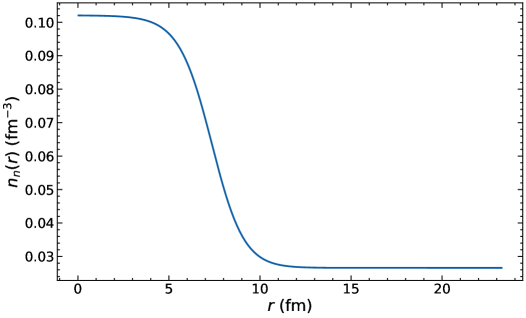
Figure 1: Neutron density distribution $n_{n}(\pmb{r})$ (in fm^-3) as function of the radial coordinate $r$ (in fermis) in the Wigner-Seitz cell in the inner crust of a neutron star at average baryon number density 0.03 fm^-3.

For the sake of comparison with previous studies, we will employ the same microscopic model as in Ref. [19]. We assume that the crust consists of a body-centered cubic lattice polycrystal of spherical clusters. We will restrict to the crustal layer at average baryon number density 0.03 fm^-3, where the suppression of the neutron superfluid density was found to be the strongest. The Wigner-Seitz cell contains $Z_{\rm cell}=40$ protons and $N_{\rm cell}=1550$ neutrons. Its radius is about $R_{\rm cell}=23.30$ fm. The lattice spacing $a$ is determined so that the volume of the exact Wigner-Seitz cell (a truncated octahedron) coincides with that of the approximate spherical cell, namely $a=R_{\rm cell}(8\pi/3)^{1/3}\approx 47.3$ fm. The neutron number density distribution is plotted in Fig. 1. The number density of free neutrons estimated from the local neutron density at the cell edge is about $n_{n,f}=2.66\times 10^{-2}$ fm^-3. This represents about 91% of the average neutron number density $\bar{n}_{n}$. The Fermi wave length $\lambda_{\rm F}=2\pi/k_{\rm F}$ of free neutrons ($k_{\rm F}=(3\pi^{2}n_{n,f})^{1/3}$ being the Fermi wave number) is about 6.8 fm. This is much smaller than the lattice spacing and comparable to the radius of the clusters, as can be seen in Fig. 1. Free neutrons are therefore expected to be Bragg diffracted by the crystal lattice and by the individual nucleons in the clusters.

We consider the existence of an average stationary neutron superflow $\bar{V}_{n,s}$ in the crust frame. As in previous studies, $\bar{V}_{n,s}$ is assumed to be much smaller than Landau’s velocity $V_{n,L}$. Expanding the neutron mass current to linear order in $\bar{V}_{n,s}/V_{n,L}$ and treating neutron pairing in the BCS approximation, the neutron superfluid density can be extracted from static band-structure calculations, as [13]

$$\rho_{n,s}=\frac{2m_{n}^{2}}{\pi^{3}\hbar^{2}}\sum_{\alpha}\int_{\rm IBZ}d^{3}\pmb{k}\,|\pmb{\nabla}_{\pmb{k}}\varepsilon_{\alpha\pmb{k}}|^{2}\frac{|\Delta_{\alpha\pmb{k}}|^{2}}{(E_{\alpha\pmb{k}})^{3}}\,,$$ (4)

where $E_{\alpha\pmb{k}}\equiv\sqrt{\xi_{\alpha\pmb{k}}^{2}+\Delta_{\alpha\pmb{k}}^{2}}$, $\xi_{\alpha\pmb{k}}=\varepsilon_{\alpha\pmb{k}}-\mu$, $\mu$ is the neutron chemical potential, $\varepsilon_{\alpha\pmb{k}}$ is the single-particle energy of the $\alpha$ band for Bloch wavevector $\pmb{k}$ obtained from the Skyrme HF equation in the absence of current

$$-\pmb{\nabla}\cdot\frac{\hbar^{2}}{2m_{n}^{\oplus}(\pmb{r})}\pmb{\nabla}\varphi_{\alpha\pmb{k}}(\pmb{r},\sigma)+U(\pmb{r})\varphi_{\alpha\pmb{k}}(\pmb{r})=\varepsilon_{\alpha\pmb{k}}\varphi_{\alpha\pmb{k}}(\pmb{r},\sigma)\,,$$ (5)

$\varphi_{\alpha\pmb{k}}(\pmb{r},\sigma)$ is the corresponding Bloch wavefunction at position $\pmb{r}$ with spin coordinate $\sigma$, and $\Delta_{\alpha\pmb{k}}$ is the solution of the anisotropic multiband BCS gap equation in the absence of current (see Ref. [37] for details). By symmetry, the $\pmb{k}$-space integration has been restricted to the irreducible wedge of the first Brillouin zone (IBZ) of the body-centered cubic lattice. The integration volume is therefore $\Omega_{\rm IBZ}=\Omega_{\rm BZ}/48$ with $\Omega_{\rm BZ}=(2\pi)^{3}/\Omega_{\rm cell}$ the volume of the full Brillouin zone (BZ) and $\Omega_{\rm cell}$ is the volume of the primitive cell in real space. The chemical potential $\mu$ is determined by the neutron number conservation

$$\bar{\rho}_{n}=\frac{6}{m_{n}\pi^{3}}\sum_{\alpha}\int_{\rm IBZ}d^{3}\pmb{k}\left(1-\frac{\xi_{\alpha\pmb{k}}}{E_{\alpha\pmb{k}}}\right)\,.$$ (6)

In the weak coupling limit $\Delta_{\alpha\pmb{k}}\ll\varepsilon_{\rm F}$ ($\varepsilon_{\rm F}=\hbar^{2}k_{\rm F}^{2}/2m_{n}$ is the Fermi energy with the Fermi wave number $k_{\rm F}=(3\pi^{2}n_{n,f})^{1/3}$), the superfluid density (4) reduces to

$$\rho_{n,s}\approx\frac{4m_{n}^{2}}{\pi^{3}\hbar^{2}}\sum_{\alpha}\int_{\rm IBZ}d^{3}\pmb{k}\,|\pmb{\nabla}_{\pmb{k}}\varepsilon_{\alpha\pmb{k}}|^{2}\delta(\varepsilon_{\alpha\pmb{k}}-\mu)\,,$$ (7)

which can be equivalently written as an integral over the irreducible domain of the Fermi surface [11]

$$\rho_{n,s}=\frac{4m_{n}^{2}}{\pi^{3}\hbar^{2}}\sum_{\alpha}\int_{\rm IBZ}|\pmb{\nabla}_{\pmb{k}}\,\varepsilon_{\alpha\pmb{k}}|d{\cal S}^{(\alpha)}\,.$$ (8)

Let us remark that an expression similar to Eq. (7) was independently derived in Ref. [38] in the context of a dilute Fermi gas in a one-dimensional optical potential.

As in our previous study [19], we ignore the spin-orbit coupling. It is very small and it was shown to alter the superfluid density at the third significant digit at most [12]. The spin-orbit coupling was also omitted in previous HFB calculations [34, 35, 36]. Each band is therefore doubly degenerate. The spin degeneracy factor $2$ has been explicitly included in the numerical factors.

In Ref. [19], the neutron superfluid density in the inner crust of a neutron star was evaluated using Eq. (8) thus ignoring pairing entirely (except for the assumption that a stationary neutron flow in the crust can exist). Here we will include pairing using Eq. (4). As shown in Ref. [37], the pairing gap averaged over the Fermi surface deviates at most by about 20% from the value obtained in uniform neutron matter at density $\rho_{n,f}$. Since the focus of this work is on the superfluid density, we will treat $\Delta_{\alpha\pmb{k}}=\Delta$ as a constant as in Refs. [31, 39] to reduce the computational cost. Varying $\Delta$ over a realistic range will allow us to assess the impact of the pairing gap on the superfluid density.

The periodic effective mass $m_{n}^{\oplus}(\pmb{r})$ and potential $U(\pmb{r})$ are constructed by superposing the corresponding mean fields of Ref. [40] calculated in the spherical Wigner-Seitz cell approximation within the self-consistent 4th-order extended Thomas-Fermi (ETF) method with proton shell correction added consistently via the Strutinsky integral (SI) theorem (the correction due to neutron-band structure was shown to be much smaller [41] and was therefore neglected). This ETFSI method is a computationally very fast approximation to the HFB equations [42]. In Refs. [31, 39], $m_{n}^{\oplus}(\pmb{r})$ was taken as the bare mass $m_{n}$ and $U(\pmb{r})$ was approximated by a fixed sinusoidal potential. The realistic fields, however, are quite different, as can be seen in Figs. 2 and 3 respectively, and this can have a strong impact on the superfluid density [10]. In the present study, the realistic fields will not be approximated. However, we will not recalculate them self-consistently since the fields obtained within the ETFSI approach were shown to be already very close to the self-consistent mean fields [42].

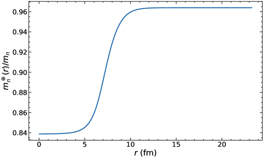
Figure 2: Local neutron effective mass $m_{n}^{\oplus}(\pmb{r})/m_{n}$ as function of the radial coordinate $r$ (in fermis) in the Wigner-Seitz cell in the inner crust of a neutron star at average baryon number density 0.03 fm^-3.

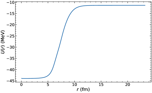
Figure 3: Local neutron potential $U(\pmb{r})$ (in megaelectronvolts) as function of the radial coordinate $r$ (in fermis) in the Wigner-Seitz cell in the inner crust of a neutron star at average baryon number density 0.03 fm^-3.

III Numerical implementation

III.1 Band-structure calculations

The HF equation (5) is solved in reciprocal space by expanding the Bloch wavefunctions into Fourier series,

$$\varphi_{\pmb{k}}(\pmb{r},\sigma)=\exp({\rm i}\,\pmb{k}\cdot\pmb{r})\sum_{\pmb{G}}\widetilde{\varphi_{\pmb{k}}}(\pmb{G})\exp({\rm i}\pmb{G}\cdot\pmb{r})\chi(\sigma)\,,$$ (9)

where $\chi$ denotes Pauli spinor and the summation is over reciprocal lattice vectors $\pmb{G}$, as imposed by the Floquet-Bloch theorem (let us recall that the reciprocal lattice of a body-centered cubic lattice is a face-centered cubic lattice). In this way, Eq. (5) is reduced to a matrix eigenvalue problem

$$\sum_{\beta}\biggl{[}(\pmb{k}+\pmb{G}_{\alpha})\cdot(\pmb{k}+\pmb{G}_{\beta})\frac{\hbar^{2}}{2\widetilde{m}_{n}^{\oplus}(\pmb{G}_{\beta}-\pmb{G}_{\alpha})}+\widetilde{U}(\pmb{G}_{\beta}-\pmb{G}_{\alpha})\biggr{]}\widetilde{\varphi}_{\pmb{k}}(\pmb{G}_{\beta})=\varepsilon_{\alpha\pmb{k}}\,\widetilde{\varphi}_{\pmb{k}}(\pmb{G}_{\alpha})$$ (10)

with the Fourier coefficients being expressed by the following integrals over any primitive cell

$$\frac{\hbar^{2}}{2\widetilde{m}_{n}^{\oplus}(\pmb{G})}=\frac{1}{\Omega_{\rm cell}}\int d^{3}\pmb{r}\,\frac{\hbar^{2}}{2m_{n}^{\oplus}(\pmb{r})}\exp(-{\rm i}\,\pmb{G}\cdot\pmb{r})\,,$$ (11)

$$\widetilde{U}(\pmb{G})=\frac{1}{\Omega_{\rm cell}}\int d^{3}\pmb{r}\,U(\pmb{r})\exp(-{\rm i}\,\pmb{G}\cdot\pmb{r})\,,$$ (12)

and with the normalization

$$\sum_{\beta}|\widetilde{\varphi_{\pmb{k}}}(\pmb{G}_{\beta})|^{2}=1\,.$$ (13)

Instead of evaluating the Bloch state velocity $\pmb{v}_{\alpha\pmb{k}}\equiv\pmb{\nabla_{k}}\varepsilon_{\alpha\pmb{k}}/\hbar$ from numerical differentiation, we have implemented the equivalent expression [2]

$$\pmb{v}_{\alpha\pmb{k}}=\sum_{\sigma}\int d^{3}\pmb{r}\,\varphi_{\alpha\pmb{k}}(\pmb{r},\sigma)^{*}\pmb{v}(\pmb{r})\varphi_{\alpha\pmb{k}}(\pmb{r},\sigma)$$ (14)

with the velocity operator

$$\pmb{v}(\pmb{r})=\frac{1}{\mathrm{i}\hbar}\biggl{[}\pmb{r}h(\pmb{r})-h(\pmb{r})\pmb{r}\biggr{]}=\frac{-{\rm i}\hbar}{2}\left(\frac{1}{m_{n}^{\oplus}(\pmb{r})}\pmb{\nabla}+\pmb{\nabla}\frac{1}{m_{n}^{\oplus}(\pmb{r})}\right)\,.$$ (15)

In numerical implementations, summations are calculated keeping a finite number of terms, $\mathcal{N}_{1}$, $\mathcal{N}_{2}$, and $\mathcal{N}_{3}$ along each basis vectors in real space or reciprocal space. We have made use of fast Fourier transforms to switch representations between real and reciprocal spaces. Since the lattice has cubic symmetry, we have chosen $\mathcal{N}_{1}=\mathcal{N}_{2}=\mathcal{N}_{3}\equiv\mathcal{N}$. The number of terms to include in the expansion cannot be arbitrarily small, but is dictated by the number of neutrons in the layer of interest. Indeed, each energy band can accommodate two neutrons (with opposite spins) per primitive cell at most (less if neutrons are paired due to the smearing of the Fermi-Dirac distribution). Therefore, $N_{\rm cell}$ neutrons per cell occupy $N_{\rm cell}/2$ bands at least. However, the maximum number of bands of the discrete eigenvalue problem (10) is limited by $\mathcal{N}^{3}$. In other words, $\mathcal{N}$ should be greater than $(N_{\rm cell}/2)^{1/3}$ to ensure that no significant violation of neutron number conservation will arise (pairing further increases the minimum number of terms although the shift is not expected to be large since most bands will still accommodate the same number of neutrons except for those lying around the Fermi level). Here $N_{\rm cell}=1550$ so that we should set $\mathcal{N}\geq 10$. Truncating the Fourier expansion implies a discretization of the real space with a spacing $\delta\ell=a/(2\mathcal{N})$ along each primitive axis, where $a$ denotes the size of the conventional cubic cell. In other words, a grid spacing $\delta\ell$ thus requires $\sim(a/2\delta\ell)^{3}$ points. Here $a=47.3$ fm. The size of the clusters is about an order of magnitude smaller, as can be seen in Figs. 2 and 3. The number of terms in the plane-wave expansion should be large enough to properly describe the internal structure of clusters since the wavefunctions of unbound neutrons must still be orthogonal to those of bound states. Unless stated otherwise, we have performed calculations using a grid of $25\times 25\times 25=15625$ points corresponding to a grid spacing $\delta\ell\approx 0.95$ fm.

In the absence of pairing, each band can accommodate two neutrons (with opposite spins) per Wigner-Seitz cell at most. Given the number $N_{\rm cell}$ of neutrons per Wigner-Seitz cell, the number of bands should thus be larger than $N_{\rm cell}/2=775$ in the present case. If neutrons are paired, the occupancy of each band is reduced due to the smearing of the Fermi-Dirac distribution and in principle summations have to be performed over all bands. However, the factor $\Delta^{2}/E^{3}$ in the integral for the superfluid fraction (4) falls rapidly whenever $\xi$ departs from $\xi=0$. For $\xi_{\rm max}\simeq 4.53\Delta$, the factor $\Delta^{2}/E^{3}$ is reduced by a hundred compared to its maximum value for $\xi=0$. In actual numerical calculations, the contribution from Bloch states with energies $\varepsilon_{\alpha\pmb{k}}>\varepsilon_{\rm max}\equiv\xi_{\rm max}+\mu$ will thus be ignored. Since the density of unbound states is given to a very good approximation by that of an ideal Fermi gas [43], the number of bands up to $\varepsilon_{\rm max}$ is roughly given by

$$\alpha_{\rm max}\equiv\alpha(\varepsilon_{\rm max})\sim Z_{\rm cell}+\frac{\Omega_{\rm cell}}{6\pi^{2}}\left[\frac{2m^{\oplus}_{B}(\varepsilon_{\rm max}-U_{B})}{\hbar^{2}}\right]^{3/2}\,,$$ (16)

where we have estimated that the number of bands corresponding to bound states is roughly equal to the number of protons per Wigner-Seitz cell (in other words, the number of bound neutrons is taken to be twice that of protons), $m_{B}^{\oplus}$ and $U_{B}$ are the mean values of the Skyrme effective mass $m_{n}^{\oplus}(\pmb{r})$ and potential $U(\pmb{r})$ in the interstitial “background” region between clusters respectively. Since the effective mass is generally smaller than the bare mass, as can be seen in Fig. 2, we can obtain an upper limit by setting $m_{B}^{\oplus}=m_{n}$. Substituting $\varepsilon_{\rm max}=4.53\Delta+\mu$ with the realistic value $\Delta=1.59$ MeV for the pairing gap (as obtained from diagrammatic calculations in neutron matter at the same average neutron density taking into account both polarization and self-energy effects [44]) and estimating the chemical potential $\mu$ using Eq. (B21) of Ref. [45] yield $\alpha_{\rm max}\sim 1265$. This rough estimate has been confirmed by extensive numerical calculations. To better assess the sensitivity of the superfluid fraction with respect to the pairing gap, we will consider lower values of $\Delta$ as well down to the limit $\Delta=0$.

III.2 Integrations over the first Brillouin zone

Integrations over the first Brillouin zone have been carried out using the special-point method [46]. The superfluid fraction integral (4) is replaced by a discrete sum over a set of points uniquely determined by the crystal structure

$$\rho_{s}\approx\frac{2m_{n}^{2}}{\pi^{3}\hbar^{2}}\Omega_{\rm IBZ}\sum_{p=1}^{p_{\rm max}}w_{p}\sum_{\alpha=1}^{\alpha_{\rm max}}|\pmb{\nabla}_{\pmb{k_{p}}}\varepsilon_{\alpha\pmb{k_{p}}}|^{2}\frac{|\Delta_{\alpha\pmb{k_{p}}}|^{2}}{(E_{\alpha\pmb{k_{p}}})^{3}}\,.$$ (17)

We have made use of the formulae given in Ref. [47] for the components of the wave vectors $\pmb{k_{p}}$ and the associated weights $w_{p}$. This method assumes that the integrand is sufficiently smooth such that the (symmetrized) Fourier components of the integrand decrease rapidly with increasing norm of the lattice vector $\pmb{\ell}$.

For very small gaps $\Delta$, the factor $\Delta^{2}/E^{3}$ is very strongly peaked around $\xi=0$ so that the special-point method becomes less reliable. In the absence of pairing $\Delta=0$, the special-point method can still provide fairly accurate results by smearing the Fermi-Dirac distribution so as to remove the discontinuity at the Fermi surface. A popular method originally developed for electronic-structure calculations is that of Methfessel and Paxton [48] based on an approximate representation of the Dirac delta distribution in terms of Hermite polynomials $H_{q}(x)$ of order $q$ ($q$ being an integer), namely

$$\delta(x)\approx D(x)\equiv 1+\frac{\exp(-x^{2})}{\sqrt{\pi}}\sum_{q=1}^{q_{\rm max}}\left(\frac{-1}{4}\right)^{q}\frac{H_{2q}(x)}{q!}\,,$$ (18)

with $x=(\varepsilon-\mu)/W$. The smearing width $W$ is a free parameter that must be suitably adjusted together with the integer $q_{\rm max}$. By construction, for any polynomial $P(x)$ of order $2q_{\rm max}+1$ or less, we have

$$\int_{-\infty}^{+\infty}dxD(x)P(x)=\int_{-\infty}^{+\infty}dx\delta(x)P(x)=P(0)\,.$$ (19)

Smearing the Fermi-Dirac distribution improves the convergence of the special-point method but requires the computation of additional bands lying above the Fermi level. The minimum number of bands to consider can be estimated similarly to Eq. (16) with $\varepsilon_{\rm max}\approx\mu+W$.

To check our implementation of the special-point method and its accuracy, we have computed the body-centered cubic lattice Green’s function for the tight-binding model defined by [49]

$$G(E)=\frac{1}{\Omega_{\rm BZ}}\int_{\rm BZ}\frac{d^{3}\pmb{k}}{E-\varepsilon_{\pmb{k}}}\,,$$ (20)

$$\varepsilon_{\pmb{k}}=\varepsilon_{0}-\varepsilon_{1}\cos(k_{x}a/2)\cos(k_{y}a/2)\cos(k_{z}a/2)\,,$$ (21)

where $\varepsilon_{0}$ and $\varepsilon_{1}$ can be expressed in terms of the tight-binding Hamiltonian. The imaginary part inside the band is related to the density of single-particle states. Without any loss of generality, we can set $\varepsilon_{0}=0$ and $\varepsilon_{1}=1$ (the general case can be treated by the suitable redefinitions: $E\rightarrow(E-\varepsilon_{0})/\varepsilon_{1}$ and $G\rightarrow\varepsilon_{1}G$). From the translational symmetry of the energy bands (in reciprocal space), the integral can be equivalently carried out over the conventional (cubic) cell, whose size is $4\pi/a$ and volume is $4\Omega_{\rm BZ}$. Recalling that the volume of the first Brillouin zone is given by $\Omega_{\rm BZ}=2(2\pi/a)^{3}$, the lattice Green’s function can thus be alternatively expressed as

$$G(E)=\frac{1}{4\Omega_{\rm BZ}}\int_{-2\pi/a}^{2\pi/a}dk_{x}\int_{-2\pi/a}^{2\pi/a}dk_{y}\int_{-2\pi/a}^{2\pi/a}dk_{z}\frac{1}{E-\cos(k_{x}a/2)\cos(k_{y}a/2)\cos(k_{z}a/2)}\,.$$ (22)

Changing variables $x\equiv k_{x}a/2$, $y\equiv k_{y}a/2$ and $z\equiv k_{z}a/2$, and making use of the fact that the cosine functions are even, the integral reduces to the more familiar form

$$G(E)=\frac{1}{\pi^{3}}\int_{0}^{\pi}dx\int_{0}^{\pi}dy\int_{0}^{\pi}dz\frac{1}{E-\cos(x)\cos(y)\cos(z)}\,.$$ (23)

This integral is known analytically and is given outside the band ($|E|\geq 1$) by [50]

$$G(E)=\frac{4}{\pi^{2}E}K^{2}\left[\sqrt{\frac{1}{2}-\frac{1}{2}\sqrt{1-\frac{1}{E^{2}}}}\right]\,,$$ (24)

where $K$ is the complete elliptic integral of the first kind defined by

$$K(u)=\int_{0}^{\pi/2}\frac{dt}{\sqrt{1-u^{2}\sin^{2}t}}\,.$$ (25)

The particular case $E=1$ is the Watson’s integral [51]:

$$G(1)=\frac{4}{\pi^{2}}K^{2}\left(\frac{1}{\sqrt{2}}\right)=\frac{1}{4\pi^{3}}\Gamma^{4}\left(\frac{1}{4}\right)\approx 1.3932\,.$$ (26)

We have evaluated Eq. (20) (with $\varepsilon_{0}=0$ and $\varepsilon_{1}=1$) numerically using the special-point method. Since $G(E)$ is independent of $a$, as shown in Eq. (23), we have set $a=1$. Note that the integrand in the lattice Green function $G(1)$ may be singular. The Watson’s integral thus provides a more stringent test of the integration scheme than for the lattice Green function for any other value $|E|>1$. Numerical estimates obtained by increasing the number of special points are displayed in Fig. 4. Using a single point [52] leads to a value fairly close to the exact result with a relative deviation of about 28% only. As shown in Fig. 5, the precision improves significantly by including a few more points: the error thus drops below 10% with 8 points. Further increasing the number of points leads to a much slower convergence towards the exact result: an estimate with a 1% precision thus requires about 3000 points. This can be traced back to the singularity of the integrand. Indeed, evaluation of the body-centered cubic lattice Green function for $E=2$ leads to an extremely fast convergence, as can be seen in Figs. 6 and 7: a precision of 3% is reached with a single point and the error falls below 0.3% by adding just another point, the exact result being $G(2)\approx 0.57915$.

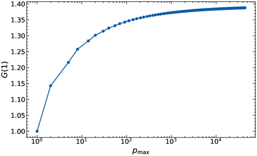
Figure 4: Watson’s integral for a body-centered cubic lattice as evaluated using the special-point method. See text for details.

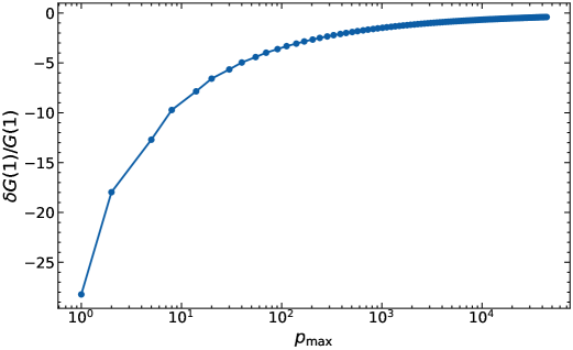
Figure 5: Relative deviation between the exact value of the Watson’s integral for a body-centered cubic lattice and its estimate from the special-point method. See text for details.

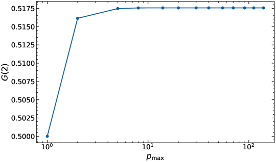
Figure 6: Body-centered cubic lattice Green function $G(2)$ as evaluated using the special-point method. See text for details.

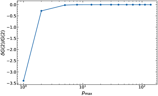
Figure 7: Relative deviation between the exact value of the body-centered cubic lattice Green function $G(2)$ and its estimate from the special-point method. See text for details.

III.3 Integrations over the Fermi surface

In the limit of very weak pairing, the special point method may become unreliable for evaluating Eq. (4) due to the very sharp variations of $\Delta^{2}/E^{3}$ with $\xi$. We have therefore computed the superfluid fraction in the limiting case $\Delta/\varepsilon_{\rm F}\rightarrow 0$ using Eq. (8). Such integrations can be accurately evaluated using the method of Gilat and Raubenheimer [53]. The irreducible domain is decomposed into identical cubic cells, whose centers are located at Bloch wave vectors $\pmb{k_{c}}$ with Cartesian coordinates $k_{cx}=(2i_{1}+1)\pi/(a\mathcal{N}_{c})$, $k_{cy}=(2i_{2}+1)\pi/(a\mathcal{N}_{c})$ and $k_{cz}=(2i_{3}+1)\pi/(a\mathcal{N}_{c})$, where $i_{1}$, $i_{2}$, and $i_{3}$ are integers satisfying $\mathcal{N}_{c}-1\geq i_{1}\geq i_{2}\geq i_{3}\geq 0$ and $i_{1}+i_{2}\leq\mathcal{N}_{c}-1$. Here $\mathcal{N}_{c}$ denotes the number of cells along the axis $k_{x}$. The total number of cubic cells in the irreducible domain is $c_{\rm max}=\mathcal{N}_{c}(\mathcal{N}_{c}+2)(\mathcal{N}_{c}+4)/24$ for $\mathcal{N}_{c}$ even and $(\mathcal{N}_{c}+1)(\mathcal{N}_{c}+2)(\mathcal{N}_{c}+3)/24$ for $\mathcal{N}_{c}$ odd. By approximating the Fermi surface intersections inside each cell by a plane, the contributions of each cell to the integral can be evaluated analytically. The superfluid fraction integral (8) is thus replaced by a discrete sum over cubic cells

$$\rho_{s}\approx\frac{m_{n}^{2}}{12\pi^{3}\hbar^{2}}\sum_{c=1}^{c_{\rm max}}w_{c}\sum_{\alpha}|\pmb{\nabla}_{\pmb{k_{c}}}\,\varepsilon_{\alpha\pmb{k_{c}}}|{\cal S}_{c}^{(\alpha)}\,,$$ (27)

where $\mathcal{S}_{c}^{(\alpha)}$ represents the area of the branch of Fermi surface from the band $\alpha$ inside the cell under consideration. Expressions for $\mathcal{S}_{c}^{(\alpha)}$ can be found in Ref. [53]. The introduction of the weights $w_{c}$ is to account for the fact that some of the cells lie outside the irreducible domain. Their determination is discussed in Ref. [54]. To test our implementation of this method, we have computed the density of states of the tight-binding model defined by

$$\mathcal{D}(E)=\int_{\rm BZ}d^{3}\pmb{k}\,\delta(E-\varepsilon_{\pmb{k}})=\int\frac{d\mathcal{S}}{|\pmb{\nabla}_{\pmb{k}}\varepsilon_{\pmb{k}}|}\approx\sum_{c=1}^{c_{\rm max}}\frac{w_{c}\,\mathcal{S}_{c}}{|\pmb{\nabla}_{\pmb{k_{c}}}\varepsilon_{\pmb{k_{c}}}|}$$ (28)

with the band energy given by Eq. (21). As shown in Fig. 8, results using 1360 cubic cells in the irreducible domain (65 280 cells in the first Brillouin zone) are found to be in excellent agreement with the interpolating formula (39c) of Ref. [55] over the whole spectrum, including in particular the Van Hove singularity at $E=0$ corresponsing to critical points for which $|\pmb{\nabla}_{\pmb{k}}\varepsilon_{\pmb{k}}|=0$.

In principle, the evaluation of Eq. (27) only requires the computation of the energies $\varepsilon_{\alpha\pmb{k_{c}}}$ in the vicinity of the Fermi level, more precisely $|\mu-\varepsilon_{\alpha\pmb{k_{c}}}|\leq\sqrt{3}\,|\pmb{\nabla}_{\pmb{k_{c}}}\varepsilon_{\alpha\pmb{k_{c}}}|\pi/(a\mathcal{N}_{c})$. However, the gradients $|\pmb{\nabla}_{\pmb{k_{c}}}\varepsilon_{\alpha\pmb{k_{c}}}|$ are difficult to reliably estimate a priori unlike the chemical potential $\mu$. With the approximation $|\pmb{\nabla}_{\pmb{k_{c}}}\varepsilon_{\alpha\pmb{k_{c}}}|\approx\hbar^{2}k_{\rm F}/m_{B}^{\oplus}$,the minimum number of bands to consider can still be reasonably well determined from Eq. (16) by substituting $\varepsilon_{\rm max}=\mu+\sqrt{3}\pi\hbar^{2}k_{\rm F}/(a\mathcal{N}_{c}m_{B}^{\oplus})$. Computations could be further reduced by ignoring bands with energies below $\varepsilon_{\rm min}=\mu-\sqrt{3}\pi\hbar^{2}k_{\rm F}/(a\mathcal{N}_{c}m_{B}^{\oplus})$. However, we have found that the results obtained in this way become less accurate with increasing number of cells. This stems from the fact that as the energy window around $\mu$ shrinks, the results become more sensitive to the errors in our rough estimate of $\varepsilon_{\rm min}$ and $\varepsilon_{\rm max}$. To avoid introducing errors that remain difficult to control, we have thus included all bands up to $\varepsilon_{\rm max}$ even though the calculations are computationally more expensive.

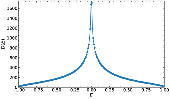
Figure 8: Density of states for the tight-binding model as calculated using the Gilat-Raubenheimer method with 1360 cubic cells (dots) and the fit (solid line) of Ref. [55].

IV Results and discussion

We first calculate the superfluid density in the limit $|\Delta_{\alpha\pmb{k}}|/\varepsilon_{\rm F}\rightarrow 0$ from Eq. (7). Brillouin-zone integrations have been performed using the special-point method with $p_{\rm max}=1360$, i.e. 65280 wave vectors in the first Brillouin zone. The Fermi-Dirac distribution is approximated by the method of Methfessel and Paxton with $30$ Hermite polynomials varying the smearing width $W$ from 0.02 MeV to 2 MeV. The number of polynomials has been increased up to $40$ but the results have not changed appreciably. We have included about 900 bands. The chemical potential is calculated using Eq. (B21) of Ref. [45]. Results are summarized in Table 1. For comparison with previous studies, the superfluid density is expressed in units of the density of free neutrons. Averaging over $W$ yields $\rho_{n,s}/\rho_{n,f}\approx 7.90\%$. Even though $W$ was varied by two orders of magnitude, the results remain remarkably stable, the deviations compared to the average value do not exceed 3%. The convergence with respect to the number of special points is shown in Fig. 9.

For comparison, Fermi-surface integrations of Eq. (8) using the more accurate Gilat-Raubenheimer method with up to 2660 cubic cells in the irreducible domain (127680 in the first Brillouin zone) including about 800 bands lead to $\rho_{n,s}/\rho_{n,f}\approx 7.91\%$, as shown in Fig. 10. The results obtained with these two completely different methods are thus found to be in excellent agreement. The Gilat-Raubenheimer method, however, is computationally less demanding and is to be preferred. This value also agrees within 7% with that obtained in Ref. [19] using a different code. We have tested the reliability of these results by recalculating the chemical potential using the special-point method. The chemical potential is not very sensitive to the detailed band structure [41]. The convergence of the superfluid fraction up to 3 significant digits has been achieved using only 70 special points in the irreducible domain (3360 wave vectors in the first Brillouin zone). The result is found to be the same as that obtained previously. We have also tested the convergence with respect to the grid spacing. Results are plotted in Fig. 11. The superfluid fraction is calculated using the Gilat-Raubenheimer method with $c_{\rm max}=1360$ (65280 cubic cells in the first Brillouin zone). The highest (lowest) resolution is reached with a FFT grid of $29^{3}=24389$ ($10^{3}=1000$) points. Fairly accurate results can be obtained with $\delta\ell\approx 1.3$ fm corresponding to a FFT grid of $18^{3}=5832$ points. Increasing $\delta\ell$ means reducing the number of plane waves describing each Bloch state. The scattering of free neutrons is therefore artificially suppressed and the superfluid fraction is exponentially enhanced. For the lowest resolution with $\delta\ell\approx 2.2$ fm, the superfluid fraction deviates from the exact result by a factor $4.3$.

Table 1: Neutron superfluid fraction in the inner crust of a neutron star calculated from Eq. (7) using 1360 special points in the irreducible domain and the smeared Fermi-Dirac distribution of Methfessel and Paxton with $30$ Hermite polynomials and different smearing widths $W$.

$W$ (MeV)	$\rho_{n,s}/\rho_{n,f}$
0.020000	0.075727
0.025485	0.077381
0.032476	0.078043
0.041383	0.075969
0.052733	0.076040
0.067196	0.077659
0.085627	0.077774
0.109112	0.078636
0.139039	0.079420
0.177173	0.078639
0.225768	0.078649
0.287690	0.078712
0.366596	0.078586
0.467144	0.078431
0.595270	0.078523
0.758538	0.078660
0.966586	0.078207
1.231696	0.078290
1.569520	0.077936
2.000000	0.077097

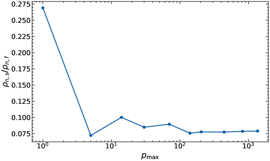
Figure 9: Convergence of the neutron superfluid fraction as calculated from Eq. (7) with respect to the number of special points.

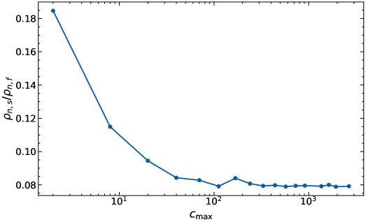
Figure 10: Convergence of the neutron superfluid fraction as calculated from Eq. (8) with respect to the number of cubic cells.

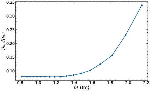
Figure 11: Convergence of the superfluid fraction with respect to the spatial grid spacing $\delta\ell$ (in fermis).

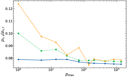
Figure 12: Convergence of the neutron superfluid fraction as calculated from Eq. (4) with respect to the number of special points. The solid curve is for $\Delta=1.59$ MeV, the dotted curve for $\Delta=0.180$ MeV, and the dashed curve for $\Delta=0.0203$ MeV.

Having assessed the precision of the special-point method for computing the superfluid fraction, we have then evaluated Eq. (17) with $p_{\rm max}=1360$ (65280 wave vectors in the first Brillouin zone) for different pairing gaps using an FFT grid of $25^{3}$ points. These calculations are computationally more demanding due to the much higher number of bands to consider, about 1300. This means computing about $2\times 10^{7}$ Bloch single-particle states. As discussed above and as can be seen in Fig. 12, the larger $\Delta$, the faster is the convergence and the more reliable are the results. For the realistic value of $\Delta=1.59$ MeV, the value of $\rho_{n,s}/\rho_{n,f}$ obtained using the mean-value point agrees within 5% with the value obtained using 1360 special points. The superfluid fractions calculated for different pairing gaps are summarized in Table 1. The relative deviations do not exceed 7% and lie within the precision of the numerical methods. In other words, the variations of superfluid fraction with the pairing gap are not significant, thus confirming earlier expectations [13]. We have checked that recalculating the chemical potential from Eq. (6) using up to $p_{\rm max}=70$ changed the numerical results for the superfluid fraction by about 1% at most for the lowest values of $\Delta$. The computational cost of the superfluid fraction can thus be substantially reduced by ignoring pairing.

Table 2: Neutron superfluid fraction in the inner crust of a neutron star for different pairing gaps $\Delta$ (in megaelectronvolts).

$\Delta$ (MeV)	$\rho_{n,s}/\rho_{n,f}$ (%)
1.59	7.51
1.11	7.51
0.770	7.52
0.535	7.55
0.372	7.60
0.259	7.66
0.180	7.70
0.125	7.74
0.0869	7.77
0.0604	7.79
0.0420	7.78
0.0292	7.78
0.0203	7.79
0.0141	7.89
0.00981	7.93

V Conclusion

We have estimated the neutron superfluid density in the inner crust of a neutron star in the limit of small neutron superfluid velocities $\bar{V}_{n,s}\ll V_{n,L}$ from fully three-dimensional neutron band-structure calculations in a body-centered cubic lattice with pairing treated in the BCS approximation. For comparison, calculations have been carried out over a range of pairing gaps including the limit of vanishing pairing. We have performed extensive numerical tests to assess the numerical precision of our code. In particular, we have computed the lattice Green function and the density of states for the tight-binding model, and compared our numerical results with known analytical expressions. We have also shown that the spatial resolution should be high enough to properly resolve the detailed structure of the Bloch wavefunctions inside the clusters and correctly describe the scattering of free neutrons by the individual nucleons in the clusters. A grid spacing $\delta\ell$ larger than about 1.3 fm leads to a spurious enhancement of the superfluid density, and the errors grow exponentially with $\delta\ell$. Setting $\delta\ell\approx 2.2$ fm overestimates the superfluid fraction by about a factor 4.

With our new code, the neutron superfluid density is found to represent about 8% of the density of free neutrons in the intermediate region of the inner crust at the average baryon density 0.03 fm^-3. This result is essentially independent of the value of the pairing gap within the numerical precision of our code. In the limit of homogeneous neutron-proton superfluid mixtures, as in the region beneath the crust of a neutron star, the HFB equations can be solved exactly. In this case, the superfluid densities were shown to be independent of the pairing gaps, no matter how strong the pairing, not only in the limit of small velocities but for any velocity not exceeding Landau’s velocity [3]. Our present calculations suggest that this conclusion also holds for an inhomogeneous superfluid.

The suppression of the superfluid fraction challenges the classical interpretation of pulsar frequency glitches in terms of neutron superfluidity in neutron-star crust  [21, 22, 23], and brings support to models involving an additional superfluid reservoir in the core. Observations of the glitch rise in the Vela and Crab pulsars point towards the interactions of the neutron superfluid vortices with proton flux tubes in the outer core of neutron stars [56].

However, the validity of the BCS approximation adopted in this work has been questioned [31, 39, 35]. In particular, Minami and Watanabe [39] compared the superfluid density calculated from the HFB equation and the BCS approximation using a three-band one-dimensional toy model with a periodic potential given by $U(x)=2V\cos(Kx)$, where $K=2\pi/a$ and $a$ is the lattice spacing. In the region of interest, $\varepsilon_{\rm F}\approx 18$ MeV and $\Delta\approx 1.6$ MeV therefore $\Delta/\varepsilon_{\rm F}\approx 0.09$. As can be seen in Fig. 3, the relative depth of the potential is about 32 MeV corresponding to $V\approx 16$ MeV and $V/\Delta\approx 10$. Looking at the blue curve in Fig. 2 of Ref. [39], which is the closest to the situation considered here, no significant difference would be expected between the BCS approximation and the full HFB equation. The validity of the BCS approximation is independently supported by the recent study of Ref. [9] in the context of a Fermi superfluid atomic condensate in an one-dimensional optical lattice with a similar periodic potential given by $U(x)=V_{0}\cos(qx)$ with $q=2\pi/d$ in their notations ($d$ is denoted by $a$ here). The authors compared the superfluid density obtained from the full HFB equations and from the weak-coupling expression (8) (which they referred to as ‘weakly interacting BCS regime’, see their Eq. (35)) varying $V_{0}$, $q=2\pi/d$, and the Fermi energy $\varepsilon_{F}$. The relevant parameters here are $V_{0}/\varepsilon_{F}\approx 1.8$, $k_{F}d\approx 44$. Looking at the black dotted curve and blue solid curve in their Fig. 3 (b) suggests again that the result of the weak-coupling approximation should be very close to that obtained from full HFB calculations. In their study, Almirante and Urban [36] considered much deeper layers of the neutron star where the neutron superfluid flows through a two dimensional lattice of parallel rod-like clusters. To compare their HFB results with those obtained in Ref. [11] in the weak-coupling approximation, the periodic effective mass $m^{\oplus}(\pmb{r})$ was set to the bare neutron mass and the potential $U(\pmb{r})$ was taken from Ref. [57]. They found that the superfluid density was sensitive to the pairing gap $\Delta$ and reduces to that of Ref. [11] only in the limit $\Delta=0$, as shown in their Fig. 6 for the average baryon number density 0.06 fm^-3. For this layer, the density of free neutrons is about $n_{n,f}\approx 5.6\times 10^{-2}$ fm^-3 and the spacing is $d=27.17$ fm for a square lattice. From Fig. 3 of Ref. [57], the depth of the potential is about $V_{0}\approx 21$ MeV. The relevant parameters are therefore $V_{0}/\varepsilon_{F}\approx 0.74$ and $k_{F}d\approx 32$. Looking again at Fig. 3 (b) of Ref. [9] suggests that the weak-coupling approximation is less accurate in this case. Therefore, the weak dependence of the superfluid fraction on the pairing gap found here at density $0.03$ fm^-3 is not necessarily in contradiction with the HFB results obtained in Ref. [36] at much higher densities. The study of Ref. [9] also provides some hint at the apparent discrepancies with previous one-dimensional calculations of the neutron superfluid fraction in slabs. From Refs. [11] and [57], we find that the typical parameters are $k_{F}d\approx 30$ and $V_{0}/\varepsilon_{F}\approx 0.37$ at the average baryon number density 0.074 fm^-3. From Fig. 3 (b) of Ref. [9], we can see that the weak-coupling approximation is more accurate than in the two-dimensional example discussed above. However, systematic three-dimensional HFB calculations with realistic self-consistent mean fields are needed to draw more definite conclusions about the role of pairing on the superfluid density in the different regions of neutron-star crusts.

Besides, the linear response theory adopted here and in previous studies certainly breaks down for superfluid velocities $\bar{V}_{n,s}\gtrsim V_{n,L}$. Superfluidity is not expected to disappear until $\bar{V}_{n,s}$ reaches a second critical velocity $V_{n,c}>V_{n,L}$ [18]. For $V_{n,L}<\bar{V}_{n,s}<V_{n,c}$, the superfluid becomes gapless and the superfluid density is further suppressed due to Cooper pair breaking [58]. Observations of transiently accreting neutron stars provide evidence for the existence of such gapless superfluid phase [59]. However, the role of the crustal lattice on those characteristic velocities and the stability of the flow remains to be investigated. This calls for further studies of the neutron superfluid dynamics in neutron-star crusts.