A Diffeomorphic Variable-Step Finite Difference Method
Abstract
This work introduces an approach to variable-step Finite Difference Method (FDM) where non-uniform meshes are generated via a weight function, which establishes a diffeomorphism between uniformly spaced computational coordinates and variably spaced physical coordinates. We then derive finite difference approximations for derivatives on variable meshes in both one-dimensional and multi-dimensional cases, and discuss constraints on the weight function. To demonstrate efficacy, we apply the method to the two-dimensional time-independent Schrödinger equation for a harmonic oscillator, achieving improved eigenfunction resolution without increased computational cost.
I Introduction
The Finite Difference Method (FDM) is a family of techniques that is a cornerstone of numerical analysis, often used to approximate the solutions to partial differential equations (PDEs) in fields as different as electromagnetism [1] [2], fluid mechanics [3] [4] and financial mathematics [5] [6]. This method relies on discretizing the parameter space in a mesh and approximate derivatives using finite differences, which effectively reduces the problem to a linear algebra one, making it significantly simpler [7]. With a sufficiently small step between gridpoints, we numerically approach the exact solution. A standard example is the one-dimensional uniform grid case. Here, we approximate the first and second order derivatives via the most simple finite differences
| (1) |
| (2) |
where it is easily seen that, in the limit where h tends to zero, Equation 1 corresponds to the definition of derivative in Calculus. For variable meshes, there are various techniques to extend this formulation for that case, and they are in general application-specific [8] [9]. Here, we shall discuss an approach to variable-mesh FDM where the grid density is given by a weight function that allows the establishment of a diffeomorphism between the computational and physical space, allowing us to solve the problem in a uniform computational space and transform the solution into the physical space. We first lay out the framework for the one-dimensional case and then build up to the higher-dimensional one. We then apply this approach to the two-dimensional time-independent Schrödinger Equation as a proof of concept.
II One-Dimensional Case
II.1 Mesh Generation
Before deriving the finite differences in a variable mesh, it is useful to define how this is constructed.
Firstly, we define a weighting function . This function gives the relative step size as a function of the position in parameter space. We say relative because due to the way we will construct the mesh, this function will always be normalized to 1, so, for instance, , where k is a constant, will yield the exact same uniformly spaced grid for any k. This function simply describes the relative density of the mesh. The function’s co-domain should lie in or any linear scaling of that. Positions in the parameter space where the value of is lower (higher) will correspond to areas with a finer (coarser) mesh. We will see later that this function essentially generates the Cumulative Distribution Function (CDF) of the mesh spacing.
Let us now say that we are trying to generate a grid of points over the interval , using the previously defined weighting function , and dividing the interval into N segments. We shall employ a mapping that transforms a uniformly spaced computational domain into our variably spaced physical domain. We hence define the computational coordinate over the interval :
| (3) |
where S(x) is the CDF of the spacing over defined from the weighting function as:
| (4) |
and is the total ”scaled” length of the interval:
| (5) |
The reasoning for this choice will become clearer later upon extrapolation to higher dimensions. For now, we note that it establishes a diffeomorphism between the computational and physical spaces, and we can freely transform between the two via this function. We can now generate uniform grid points in -space by dividing its domain into N equal segments as:
| (6) |
and map these points from the computational grid onto the physical grid via the relation:
| (7) |
where might not always have an analytical inverse, but it can be easily found via numerical methods in a practical implementations.
II.2 Finite Differences
Let be three consecutive points, let be the distance between and and let be the distance between and . We want to derive the finite differences that approximate the derivatives of a function in a discrete mesh using a central approximation at a point . Here, we derive the first- and second-order derivatives, but the same principle applies further. We want to find the coefficients where i=1,2, such that:
| (8) |
| (9) |
We then substitute and with their respective Taylor series expansions around :
| (10) |
| (11) |
Solving, we find that the coefficients are
| (12) | ||||
and
| (13) | ||||
Therefore, the general form of the finite differences with variable mesh becomes, for the first derivative:
| (14) |
and for the second derivative:
| (15) |
One can easily see that in the case of a uniform grid, , and hence
| (16) |
| (17) |
and we retrieve the known form for a constant-step mesh as in Equations 1 and 2.
III Generalization to Higher Dimensions
III.1 Mesh Generation
III.1.1 General weight function
In the case of multiple dimensions, analogously to the method previously described for a single dimension, our aim is to map a uniformly spaced computational domain to the physical domain , according to the weight function . We can define the map between the computational and physical spaces by considering the divergence of a vector field in computational space:
| (18) |
where is a tensor that incorporates the grid density, and in our case it is generated by the weight function as
| (19) |
where is the identity tensor. This yields the form of the grid generation equations given a fully general -dimensional
| (20) |
which is a system of coupled PDEs for . Note that for , this reduces to a single equation
| (21) |
| (22) |
where by integrating and identifying C as , we can easily retrieve the form in Equation 3. To ensure that the diffeomorphism between computational and physical spaces holds, we must set that should be integrable everywhere in the domain, different from zero for any and be bounded, such that .
III.1.2 Separable weight function
In the case where is separable:
| (23) |
the grid generation equations can be decoupled into a set of independent PDEs
| (24) |
We can simplify this further as
| (25) |
where are constants. Finally, integrating, we arrive at the relation
| (26) |
where is completely analogous to the definition introduced in Equation 4
| (27) |
We note that separability allows for an independent and one-dimensional treatment of each dimension, which greatly simplifies the mesh generation problem. For that reason, it might be desirable in most cases to use weight functions of this type to speed up and simplify the grid generation. It is easy to see that can be identified with the normalization constant of the weight function in each dimension , and hence we fully retrieve our treatment for the one-dimensional case as described in Equation 7.
III.2 Finite Differences
For ease of notation, let’s define
| (28) |
Consider that we have generated the grid points , where index the grid in the directions. The step sizes in the direction are, analogously to the one-dimensional case:
| (29) |
| (30) |
And equivalently for all other dimensions. Following a process analogous to the one shown for the one-dimensional case, we find that the finite difference approximations to the first and second derivatives are given by Equations 31 and 32 respectively. Note that these Equations give the form for the partial derivatives with respect to , but this is perfectly extendable to any other variable by simply replacing with the variable of interest and affecting the respective index instead of .
| (31) |
| (32) |
IV Example of Implementation
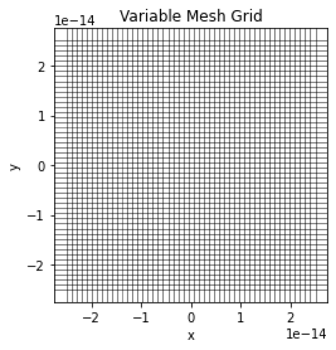
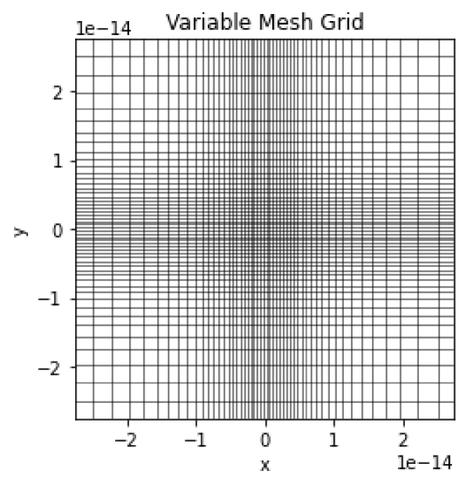
We shall use a grid of points in both cases, meaning that the Hamiltonian matrix of this eigenvalue problem has the same size in both cases, so the problems are computationally equivalent. The weight functions used were:
| (33) |
| (34) |
The resulting mesh is shown in Figure 1(b), next to the uniform mesh, for comparison.
The two-dimensional time-independent Schrödinger equation is given by [10]:
| (35) |
Which can be formulated in the form of an eigenvalue problem , by defining a Hamiltonian operator
| (36) |
For a harmonic oscillator, we use the potential
| (37) |
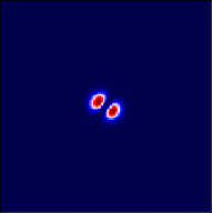
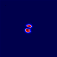
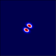
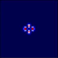
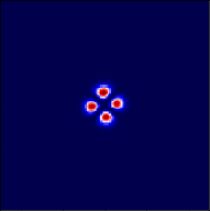
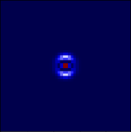
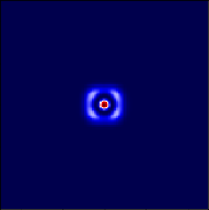
For this example, we shall discretize the two-dimensional phase space in 50 steps. As for the potential, we use the form described in Equation 37 using and . We can discretize Equation 35 using the finite difference scheme described in Equation 32.
| (38) | ||||
By treating as a matrix, we separate the left-hand-side into an matrix multiplying by , and arrive at the well-known eigenvalue problem form
| (39) |
which was then solved using Python.
 |
 |
| (1) | |
 |
 |
| (2) | |
 |
 |
| (3) | |
 |
 |
| (4) | |
 |
 |
| (5) | |
V Conclusions
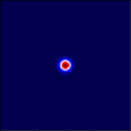
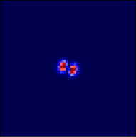
We have derived a formalism that allows the application of the Finite Difference Method using a variable mesh through a relative mesh spacing weight function . This formalism is presented for both the one-dimensional and arbitrary-dimensional case. We have shown an example of application by solving the two-dimensional Schrödinger equation using both uniform and variable mesh, with the same average step size, observing how this formalism can be a useful tool to better resolve the eigenfunctions of this Hamiltonian, which are very localized at the center of the parameter space, without necessarily increasing the computational cost, since ultimately the total size of the Hamiltonian matrix whose eigenvalues and eigenfunctions we are solving for is the same for both.
References
- Kunz and Luebbers [1993] K. S. Kunz and R. J. Luebbers, The finite difference time domain method for electromagnetics (CRC press, 1993).
- Zhou [1993] P.-b. Zhou, Numerical Analysis of Electromagnetic Fields (Springer Berlin Heidelberg, 1993).
- Godunov and Bohachevsky [1959] S. K. Godunov and I. Bohachevsky, Finite difference method for numerical computation of discontinuous solutions of the equations of fluid dynamics, Matematičeskij sbornik 47, 271 (1959).
- Narasimhan and Witherspoon [1976] T. Narasimhan and P. Witherspoon, An integrated finite difference method for analyzing fluid flow in porous media, Water Resources Research 12, 57 (1976).
- Duffy [2013] D. J. Duffy, Finite difference methods in financial engineering: a partial differential equation approach (John Wiley & Sons, 2013).
- Hull and White [1990] J. Hull and A. White, Valuing derivative securities using the explicit finite difference method, Journal of Financial and Quantitative Analysis 25, 87–100 (1990).
- Grossmann et al. [2007] C. Grossmann, H.-G. Roos, and M. Stynes, Numerical Treatment of Partial Differential Equations (Springer Berlin Heidelberg, 2007).
- Perrone and Kao [1975] N. Perrone and R. Kao, A general finite difference method for arbitrary meshes, Computers & Structures 5, 45–57 (1975).
- Kadalbajoo and Kumar [2010] M. K. Kadalbajoo and D. Kumar, Variable mesh finite difference method for self-adjoint singularly perturbed two-point boundary value problems, Journal of Computational Mathematics , 711 (2010).
- Schrödinger [1926] E. Schrödinger, An undulatory theory of the mechanics of atoms and molecules, Physical Review 28, 1049–1070 (1926).