Impact of the exciton fine structure splitting and measurement orientations
on the robustness of cryptographic keys generated via the quantum protocol E91

Abstract

Photons and optical circuits are among the most promising platforms for implementation of quantum technologies, because of its potential use in quantum computing, quantum cryptography and long-distance quantum communication. One of the main requirements to achieve reliable quantum communications are on-demand sources of highly entangled photon pairs, and semiconductor quantum dots have emerged as prominent candidates to satisfy the necessary conditions of brightness and entanglement fidelity. However, in most cases the biexciton-exciton-vacuum cascade produces a pair of maximally polarization-entangled photons with a dephasing, due to the exciton fine structure splitting. This work focuses on the performance of the E91 quantum key distribution protocol under the variation of two elements: first, the phase in the input state when the protocol is implemented using entangled photons generated via the radiative cascade, and second, the relative directions of the polarization analyzers. We obtain analytical expressions for the protocol’s secret key rate and Bell’s parameter as functions of the studied phase and angles. Then, we validate those expressions by means of a quantum computational implementation with the IBM’s API Qiskit. Our results show that the performance of the quantum transmission is highly impacted by the product between the exciton lifetime and the quantum dot’s fine structure splitting and that such an impact may be modulated through the orientation of the polarizers. These findings provide important insight for the scalable implementation of quantum key distribution protocols with quantum dots as entanglement sources.

I Introduction

Quantum key distribution (QKD) is a private-key cryptographic model that exploits the principles of quantum mechanics such as superposition, entanglement, and collapse of quantum states; to transmit quantum bits that conform a cryptographic key to encrypt and decrypt information [1, 2, 3, 4]. Realization of this cryptographic model has been achieved mainly with the use of optical quantum entangled states, what has promoted the photonic implementation as a realistic option for quantum communication and quantum internet [5, 6, 7, 8, 9, 10]. Thus, the development of optimized entangled-photon sources has become a topic of intense research toward the progress of light-based quantum technologies [11, 12, 13, 14].

Quantum entangled states were widely discussed and subject of controversy during the second part of the XX century since their introduction by Einstein, Podolsky, and Rosen [15]. Arguably the main contribution toward resolving the dispute on the reality of those perplexing states, was provided by J. Bell who mathematically proved that any hidden variable theory is incompatible with the statistical predictions of quantum mechanics, its result is known as the Bell’s Theorem [16]. Later on, other authors recreate their own versions of that theorem, raising a set of expression named Bell inequalities. Particularly, Clauser et al. in reference [17], develop a theorem known as the CHSH inequality. This inequality has been experimentally verified via photon-based experiments in which, first, a radiative cascade decay in calcium atoms, and later, spontaneous parametric down conversion (SPDC) in nonlinear crystals, were used as entangled-photon sources [18, 19, 20, 21].

The so-called E91 protocol was the first quantum entanglement-based QKD protocol, devised by A. K. Ekert in the early 90’s. [22, 23]. In the original version of the protocol, the author proposed the use of $1/2$-spin particles prepared in a Bell’s state. Nevertheless, at the last part of that seminal work, he mentioned that an optimal realization could be based on correlated photon states. This protocol includes a mechanism for validating the security of the transmitted key, based on measurements of the Bell’s theorem to rule out eavesdropping. That verification mechanism is normally implemented in terms of the CHSH inequality. This QKD scheme was first effectively implemented by using polarization-entangled photon states produced via SPDC. Afterwards, entangled photons obtained from semiconductor quantum dots (QDs) were used, achieving long-distance transmission, although the yielded key was found below what could be achieved with a SPDC source [6, 24, 25, 21, 26, 27].

SPDC has been so far the most commonly employed mechanism for entanglement generation, because of the highly entangled photons obtained by this method [28]. Nevertheless, its production of photon pairs is random and then unsuitable for reliable quantum communication, or other applications that require an on-demand source of entangled states. In this scenario, QDs have appeared as promising candidates for optimal on-demand entanglement generation. In fact, there have been several successful implementations of long-distance QKD with QDs as entangled-photon sources [29, 8, 30, 27, 31, 32, 33, 34]. Nevertheless, QD-produced entangled states are frequently dephased with respect to the ideal Bell states for which the QKD protocols are usually designed. Such a dephasing is underlaid by the so-called electron-hole exchange, that causes the exciton fine structure splitting (FSS) in strongly confined nanostructures [35, 36, 37, 38].

In this work we study the effects of the FSS-driven dephasing in the entangled input state and those of the relative orientation between measurement axes on the performance of the E91 QKD protocol. In the first part, we introduce the dephasing effects of the FSS on the entangled states produced in QDs. Afterward, we explore the influence of both, the FSS-driven dephasing and the orientation of the detection axes, in the execution of the QKD protocol E91, and derive the corresponding analytical expressions. Finally, by using a quantum computing implementation, we validate our model and discuss the impact of the analyzed variables on the performance of the key distribution process.

II Sources of entangled photon pairs for QKD

Many of the fundamental experiments that allowed to verify the physical reality behind entanglement, as well as most of the QKD experiments carried out to date, have used SPDC to produce quantum correlated photons [6, 5, 39, 7, 40]. This mechanism permits the creation of a pair of lower-energy daughter photons originated from a higher-energy pump photon, that interacts with a transparent non-linear crystal inside which it is randomly split into an polarization entangled pair [41]. Because SPDC is not an on-demand process, its use for implementations of scaled quantum communication is dubious. The probability of obtaining entangled pairs given an incident photon, is described by a Poissonian distribution. Hence, probabilistically none, one or several pairs of entangled photons may be produced, being none much more likely under normal conditions than the other components. Thus, the efficiency of this entanglement-generation method is very low and its potential for applications in emerging quantum technologies, clearly limited [42, 43, 44].

Instead of a stochastic source, quantum dots have been proposed as a deterministic on-demand source of highly entangled photon pairs by exploiting the recombination of the biexciton state ($\left|XX\right\rangle$). This process yields two polarization-entangled photons that, in contrast to SPDC, can be successfully applied in quantum communications [29, 35, 45, 46, 47]. Nevertheless, the coherence of the entangled polarization state may be altered as a result of the interactions between the produced photons and its environment, such as recapture or depolarization by defects; or as consequence of the exciton fine structure associated to intrinsic characteristics of the emitting QD. In particular, this latter effect has been widely studied and identified as the main challenge toward reliable generation of entangled states from QDs. The dephasing introduced by the FSS into the entangled output state, is known to directly depend on that energy splitting between the exciton states ($\left|X,-1\right\rangle$ and $\left|X,1\right\rangle$) [48, 45, 46, 38].

II.1 Entangled photon pairs from radiative cascades in QDs

The process starts with excitation of the neutral biexciton state $\left|XX\right\rangle$, that later decays into one of the single exciton states $\left|X\right\rangle$ by one of two possible decay routes (either to $\left|X,-1\right\rangle$ and $\left|X,1\right\rangle$). Through the first pathway, a photon with right circular polarization $\left|R_{XX}\right\rangle$ is emitted and the system’s $z$-component of angular momentum passes from $m=0$ to $m=-1$ (decaying to the state $\left|X,-1\right\rangle$). Contrarily, through the second pathway, the emitted photon has left circular polarization $\left|L_{XX}\right\rangle$ and the system passes from $m=0$ to $m=1$ (decaying to the state $\left|X,1\right\rangle$). Afterwards, the corresponding exciton state decays into the ground state ($\left|0\right\rangle$) emitting a photon with opposite polarization respect to the previously emitted, and the system returns to $z$-component of total angular momentum $m=0$ [35, 49]. This radiative cascade and its two pathways are depicted in figure 1, where cyan (orange) represents emission of a right (left) circularly polarized photon and $S$ stands for the FSS energy.

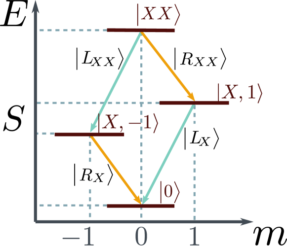
Figure 1: Radiative cascade $\left|XX\right\rangle\to\left|X\right\rangle\to\left|0\right\rangle$ in a quantum dot. There are two different decay routes, one through state $\left|X,-1\right\rangle$ ($m=0\rightarrow m=-1\rightarrow m=0$) and the other one through state $\left|X,1\right\rangle$ ($m=0\rightarrow m=1\rightarrow m=0$). The cyan (orange) line represents emission of a right (left) circularly polarized photon.

In the case $S=0$, the two decay pathways are indistinguishable. However, if $S\neq 0$ the degeneracy of exciton states with different angular momentum is lifted. This makes the decay routes distinguishable and the two-photon entangled state becomes

$$|\psi\rangle\,=\,\dfrac{1}{\sqrt{2}}\left[|L_{XX}R_{X}\rangle+e^{-i\theta_{\text{FSS}}}|R_{XX}L_{X}\rangle\right],$$ (1)

where the relative phase $\theta_{\text{FSS}}=S\tau/\hbar$, with $\tau$ being the time between the first and second electron-hole recombination (neutral exciton radiative lifetime). [50, 35, 51].

This state is maximally entangled disregarding the value of $\theta_{\text{FSS}}$, because the relative phase does not affect the Von Neumann entropy of the system. Nevertheless, such a dephasing creates an oscillation between Bell states along time. In other words, the electron-hole exchange induces via the $FSS$, a local unitary transformation over the Bell singlet state in the Poincare’s sphere that affects its stationary character [52, 53, 54, 38, 55].

The state in equation (1) can be rewritten in terms of linear horizontal (H) and vertical (V) polarizations, according to

$$|\psi\rangle\,=\,\dfrac{1}{\sqrt{2}}\left[|H_{XX}H_{X}\rangle+e^{-i\theta_{\text{FSS}}}|V_{XX}V_{X}\rangle\right].$$ (2)

Tuning of the FSS in QDs has been a field of intense research, since the related dephasing produces time dependent oscillations in the fidelity, hurting the possibility of determining the degree of entanglement of the emitted states [56].

Different ways of reducing the $S$ energy in QDs have been proposed, aiming to reshape the wave function of the confined carriers, to compensate the asymmetries that strengthen the magnitude of the electron-hole exchange interaction [57, 58, 59, 60].

Although successful QD tuning has been realized using either piezoelectric substrates or stark effect with external electric fields [61, 45, 62, 63, 13], still most grown QD samples exhibit non-vanishing FSS due to the inherent lack of rotational symmetry associated to both, the microscopic crystalline structures and the non-perfectly axial dot shapes.

III QKD protocol E91

The original E91 protocol aims the communication of a private key between two distant subjects, Alice and Bob, encoded on the spin of a pair of entangled $1/2$-spin particles prepared on a singlet state. However, Ekert ended suggesting that an optical implementation could be more suitable [22, 2]. Such implementation with photons was actually realized around a year later [6]. The protocol begins with the preparation of a polarization-entangled Bell state, then one photon is sent to Alice and the other one to Bob. Each participant is expected to measure his/her corresponding particle with adjustable polarizers. Each apparatus (Alice’s and Bob’s) can be set in 3 possible directions that are part of a group of 4 preset orientations, defined by its angle with respect to vertical axis. These orientations are labeled $\phi_{i}$, $i=0,1,2,3$, and their angles in the photonic version of the original protocol are defined according to $\phi_{\ell}=\ell\pi/8$ for $\ell=0,1,2,3$, as illustrated in figure 2(a).

Afterwards, Alice randomly selects one of the first three directions and registers her choice ($\phi_{i_{A}}$). Then, measures the particle and records either $-1$ or $1$, depending on the result of her measurement.

In turn, Bob selects one of the last three directions, and also records his chosen orientation ($\phi_{i_{B}}$) and the corresponding measurement.

In this form, the second and third directions among the set of four ($\phi_{1}=\pi/8$ and $\phi_{2}=\pi/4$), are part of the Alice’s and Bob’s possibilities, and then, the ones in which there can be coincidence. Once the transmission has concluded, each participant shares on a public channel, his/her list with the selected orientations for each event. Each participant analyzes the other’s list and compares it with his/her own to separate his/her registered measurements in 2 groups: the first contains the measurements for which Alice and Bob chose the same direction, and the second includes the ones where they mismatch the orientation. The cryptographic key is the string of results in the first group, while the second group of measurements is employed to validate the security of the key distribution via Bell’s test on the CHSH inequality. Such particular angles defined as multiples of $\pi/8$ were intentionally picked to maximize the quantity

$$CR=E(\phi_{0},\phi_{1})+E(\phi_{2},\phi_{3})+E(\phi_{0},\phi_{3})-E(\phi_{2},\phi_{1}),$$ (3)

given in terms of the correlation amplitudes

$$\begin{split}E(\phi_{a},\phi_{b})=-\cos\left[2(\phi_{a}-\phi_{b})\right].\end{split}$$ (4)

Such a quantity is used for the Bell’s test, carried out in the validation stage of the protocol when eavesdropping is considered. For those specifically chosen angles $CR=-2\sqrt{2}$ [2, 17, 6, 55].

III.1 Modifications to the E91 protocol and analytical results

We now consider a polarization-entangled state of photons produced via a QD radiative cascade, as described in section II. Additionally, we include a generalization by defining the detection orientations $\phi_{1}$ and $\phi_{2}$ in terms of variable angles.

Thus, we introduce the parameter $\alpha$, as the angle between the vertical axis and the second orientation in the set of four ($\phi_{1}$). Similarly, we define the parameter $\beta$ as the angle between the two coincident directions ($\phi_{2}-\phi_{1}$). These parameters are highlighted respectively in cyan and orange, in figure 2(b).

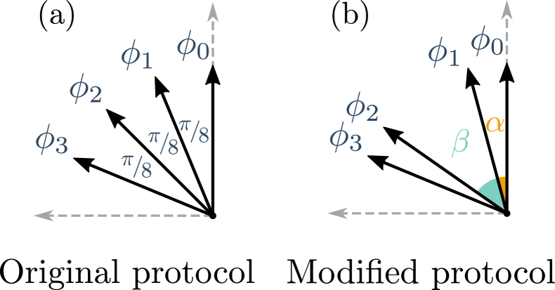
Figure 2: Angles for the optical implementation of the E91 protocol. (a) Fixed measurement directions in the originally proposed version of the protocol. (b) Variable measurement directions in the modified version of the protocol.

If we consider two bases, i.e. the vertical-horizontal and the $\phi$-rotated-$\phi$-antirotated linear polarizations, for a Bell state of polarization-entangled photons $\dfrac{1}{\sqrt{2}}\left[|H_{XX}H_{X}\rangle+|V_{XX}V_{X}\rangle\right]$ ($\theta_{\text{FSS}}=0$), measurements on both photons are certainly correlated if they are obtained in the same basis (along the same orientation), disregarding the angle $\phi$ between those bases [64].

However, if the dephasing associated to the FSS is included ($\theta_{\text{FSS}}\neq 0$), the probability of correlation will depend on the rotation angle, according to

$$P_{\pm\pm}(\phi,\theta_{\text{FSS}})=\Big{[}C_{\phi}^{4}+S_{\phi}^{4}+2S_{\phi}^{2}C_{\phi}^{2}C_{\theta_{\text{FSS}}}\Big{]},$$ (5)

where $S_{\phi}=\sin(\phi)$ and $C_{\phi}=\cos(\phi)$. $P_{\pm\pm}$ stands for the probability of obtaining either ${}^{1}_{1}$ or ${}^{-1}_{-1}$ in both (Alice’s and Bob’s) measurements. The detailed derivation is presented in Appendix A.

The probability of equation (5) is essential to compute the performance of the QKD protocol under the effects of the exciton FSS in the QD source. We can use now this expression to compute the total probability of getting correlated measurements in an event in which the bases chosen by Alice and Bob coincide, even if none of those bases correspond to the vertical-horizontal one. Such probability is the addition of the probability when both participants chose $\phi_{1}$ plus the probability when they choose $\phi_{2}$, namely

$$\begin{split}P_{\text{Corr}}\,=&\,P_{\phi_{1}}\left[P_{\pm\pm}(\phi_{1},\theta_{\text{FSS}})\right]+P_{\phi_{2}}\left[P_{\pm\pm}(\phi_{2},\theta_{\text{FSS}})\right],\end{split}$$ (6)

where $P_{\phi_{i}}$ for $i=1,2$ is the probability of choosing $\phi_{i}$ as the measurement orientation in a coincident event. Since the election of basis before each measurement is random, then $P_{\phi_{1}}=P_{\phi_{2}}=\frac{1}{2}$.

In the optical implementation of the original protocol ($\phi_{1}=\pi/8$ and $\phi_{2}=\pi/4$), this total probability turns into

$$\begin{split}P_{\text{Corr}}\,=&\frac{5+3C_{\theta_{\text{FSS}}}}{8}.\end{split}$$ (7)

As expected, if the FSS vanishes $P_{\text{Corr}}=1$, and the protocol would work optimally in absence of eavesdropping.

For the more general case of the modified protocol, in which the angles defining $\phi_{1}$ and $\phi_{2}$ are variable, the total probability of correlation for measurements along the coincident orientations, reads

$$P_{\text{Corr}}\, = \,\dfrac{1}{2}\left[P_{\pm\pm}(\alpha,\theta_{\text{FSS}})+P_{\pm\pm}(\alpha+\beta,\theta_{\text{FSS}})\right],$$ (8)

$$= \dfrac{1}{2}\Big{[}C_{\alpha}^{4}+S_{\alpha}^{4}+2S_{\alpha}^{2}C_{\alpha}^{2}C_{\theta_{\text{FSS}}}+$$

$$\hskip 4.30554ptC_{\alpha+\beta}^{4}+S_{\alpha+\beta}^{4}+2S_{\alpha+\beta}^{2}C_{\alpha+\beta}^{2}C_{\theta_{\text{FSS}}}\Big{]}.$$

This expression allows to straightforwardly predict the effects of both, the FSS in the entanglement’s source and the directions of the coincident detectors, on the performance of the considered QKD protocol.

It is important to note that according to this result, while the angles $\alpha$ and $\beta$ are irrelevant in the case $\theta_{\text{FSS}}=0$, they become determining on the effectiveness of the protocol when the FSS is not negligible.

Regarding the Bell quantity ($CR$), it is not a fixed value but rather a function that depends on $\alpha$, $\beta$ and $\theta_{\text{FSS}}$. It can be expressed as

$$\begin{split}CR=&C_{\theta_{FSS}}S_{2(\alpha+\beta)}\left[\dfrac{1}{\sqrt{2}}+S_{2\alpha}\right]+C_{2(\alpha+\beta)}\left[C_{2\alpha}-\dfrac{1}{\sqrt{2}}\right]\\ +&C_{2\alpha}+\dfrac{1}{\sqrt{2}}.\end{split}$$ (9)

The details of the derivation are given in Appendix A.

For the orientations originally proposed by Ekert (in the optical implementation), the equation 9 reduces to

$$\left|\left\langle CR\right\rangle\right|=\sqrt{2}\left|C_{\theta}+1\right|\leq 2\sqrt{2}.$$ (10)

Thus, although $CR$ is still bounded by $\pm 2\sqrt{2}$, it oscillates as $\theta_{\text{FSS}}$ increases, exhibiting minima ($CR=0$) for $\theta_{\text{FSS}}=n\pi$ ($n$ integer $>0$).

IV Computational implementation

To test the validity of equation (8), we opt for a quantum computational implementation that simulates the QKD through the considered protocol. To build a quantum algorithm that emulates the quantum transmission of the key, we first encoded the polarization states into the qubit representation by using the computational basis and rotations gates, as shown in table 1.

Table 1: Photon information encoded on quantum computation language

Scheme	Unrotated Basis	Rotated Basis
PhotonPolarization	$\big{\{}\left|H\right\rangle,\left|V\right\rangle\big{\}}$	$\Big{\{}e^{i\phi_{\ell}\hat{Y}/2}\left|H\right\rangle,e^{i\phi_{\ell}\hat{Y}/2}\left|V\right\rangle\Big{\}}$
QuantumComputation	$\big{\{}\left|0\right\rangle,\left|1\right\rangle\big{\}}$	$\Big{\{}\hat{R}_{y}(\phi_{\ell})\left|0\right\rangle,\hat{R}_{y}(\phi_{\ell})\left|1\right\rangle\Big{\}}$

To reach this goal, we rewrite the dephased singlet state in the computational basis for two qubits, generated by the operator $\hat{Z}\otimes\hat{Z}$, where the parametrized relative phase is added by applying the $R_{z}$-gate over anyone of the two qubits [50]. Thus, the state of equation (2) reads

$$|\psi\rangle\,=\,\dfrac{1}{\sqrt{2}}\left[|00\rangle+e^{-i\theta_{\text{FSS}}}|11\rangle\right].$$ (11)

IV.1 Quantum algorithm

Once the encoding is defined, we focus on creating a quantum circuit that: First, recreates the transmission of a pair of entangled qubits in the state of equation (11). Second, mimics the process of basis selection performed by Alice and Bob, and saves the chosen direction. Third, measures the quantum channels and stores the values registered by each participant.

The quantum circuit implemented to emulate the generation and transmission of one key-bit is depicted in figure 3. There, the quantum gates $\boxed{X}$, $\boxed{H}$, $\boxed{R_{Z}}$, $\dot{\oplus}$ and $\boxed{R_{Y}}$, respectively represent the Pauli_X, Hadamard, $Z$-rotation, Controlled-$X$ and $Y$-rotation unitary operations.

The circuit starts by producing the dephased entangled state in terms of $\theta_{\text{FSS}}$ (green stage), and then introduces the random selection of the direction in which each participant carries out his/her measurement (pink stage). Event by event (associated to each entangled input state), they choose among their corresponding three available directions ($\phi_{i}$ with $i=0,1,2$ for Alice and $\phi_{j}$ with $j=1,2,3$ for Bob), which are defined in terms of the parameters $\alpha$, and $\beta$, according to the orientations shown in 2(b). The implementation of the latter involves a couple of $\boxed{R_{y}(\phi_{\ell})}$ rotation gates, that are applied over the quantum channels to emulate the rotation of the polarization detectors, right before the associated measurements. Each measurement may yield either a 0 or a 1, which are correspondingly mapped to -1 or 1, in the language of equation (5).

Each of these events may become one of the bits in the key-string as long as the bases chosen by Alice and Bob coincide. Hence, to achieve a key with a number of bits long enough, the described process must be repeated a large number of times.

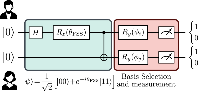
Figure 3: Quantum circuit for the transmission of a bit of information using the modified E91 scheme. In the green stage the dephased Bell state is created and in the pink stage, Alice and Bob carry out the measurements along the directions $\phi_{i}$ and Bob $\phi_{j}$, respectively, with $i=0,1,2$ and $j=i+1$. Each measurement may yield either 0 or 1, which are respectively mapped to the -1 or 1 possibilities in the original protocol.

To evaluate the performance of the quantum distribution, we chose the secret key rate ($SKR$) as a convenient metric. This is computed by counting the key-beats successfully transmitted. i.e. key-bits effectively correlated (the same for Alice and Bob in an event in which they chose coincident basis). Readily

$${\small SKR\,=\,\dfrac{\text{Number of correlated bits in the key-string}}{\text{Number of events measured in coincident basis}}.}$$ (12)

A complementary metric is the so-called quantum bit error rate ($QBER$), that oppositely to the $SKR$, focus on the number of bits transmitted with error (anticorrelated or unmeasured), in an event in which Alice and Bob chose coincident bases. In this case in which eavesdropping and leaking is not considered, $QBER=1-SKR$.

In the final stage of the computational implementation, the $SKR$ value is registered as a function of the parameters $\alpha$, $\beta$ and $\theta_{\text{FSS}}$.

V Simulation Results and Discussion

We execute the algorithm described in the previous section, to replicate the modified version of E91 protocol by means of the IBM’s Qiskit Aer simulator [65]. We opted for executing it in a quantum simulator instead of an actual quantum processor to avoid the effects of noise, which we expect to incorporate into the model in a further work.

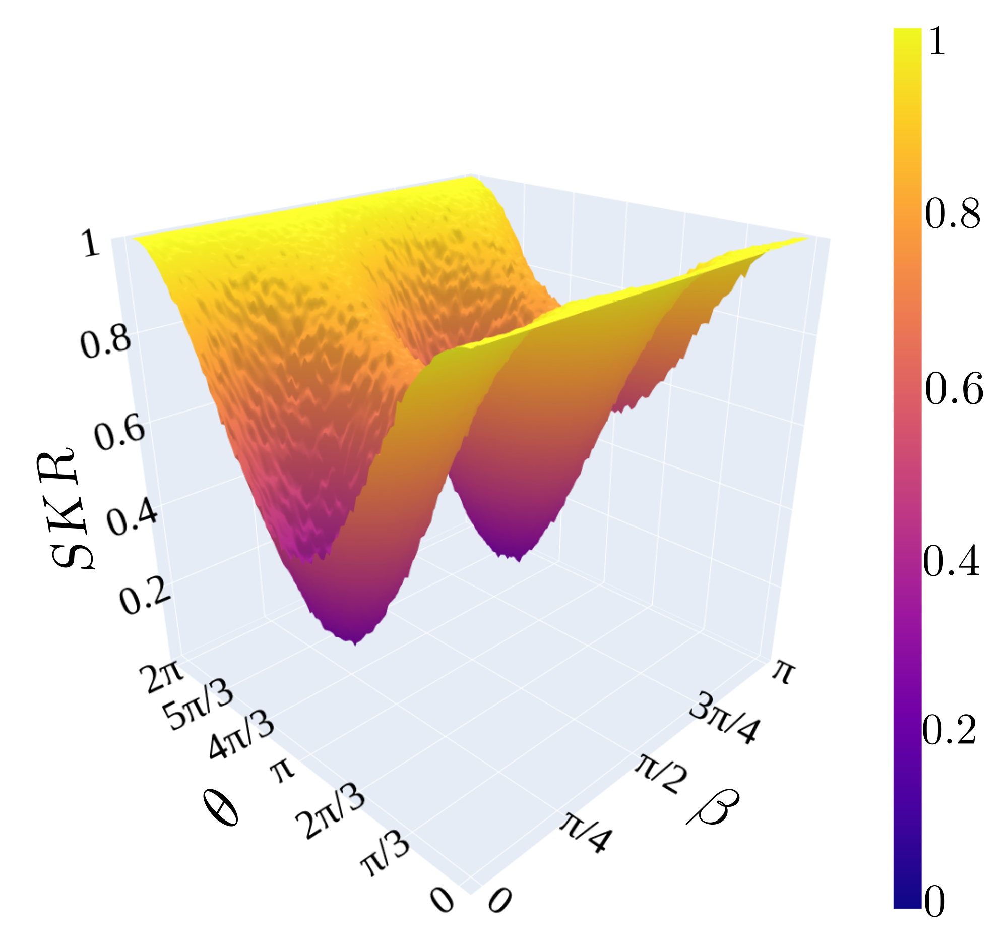
(a) $\alpha=\pi/8$. $R^{2}=0.997$

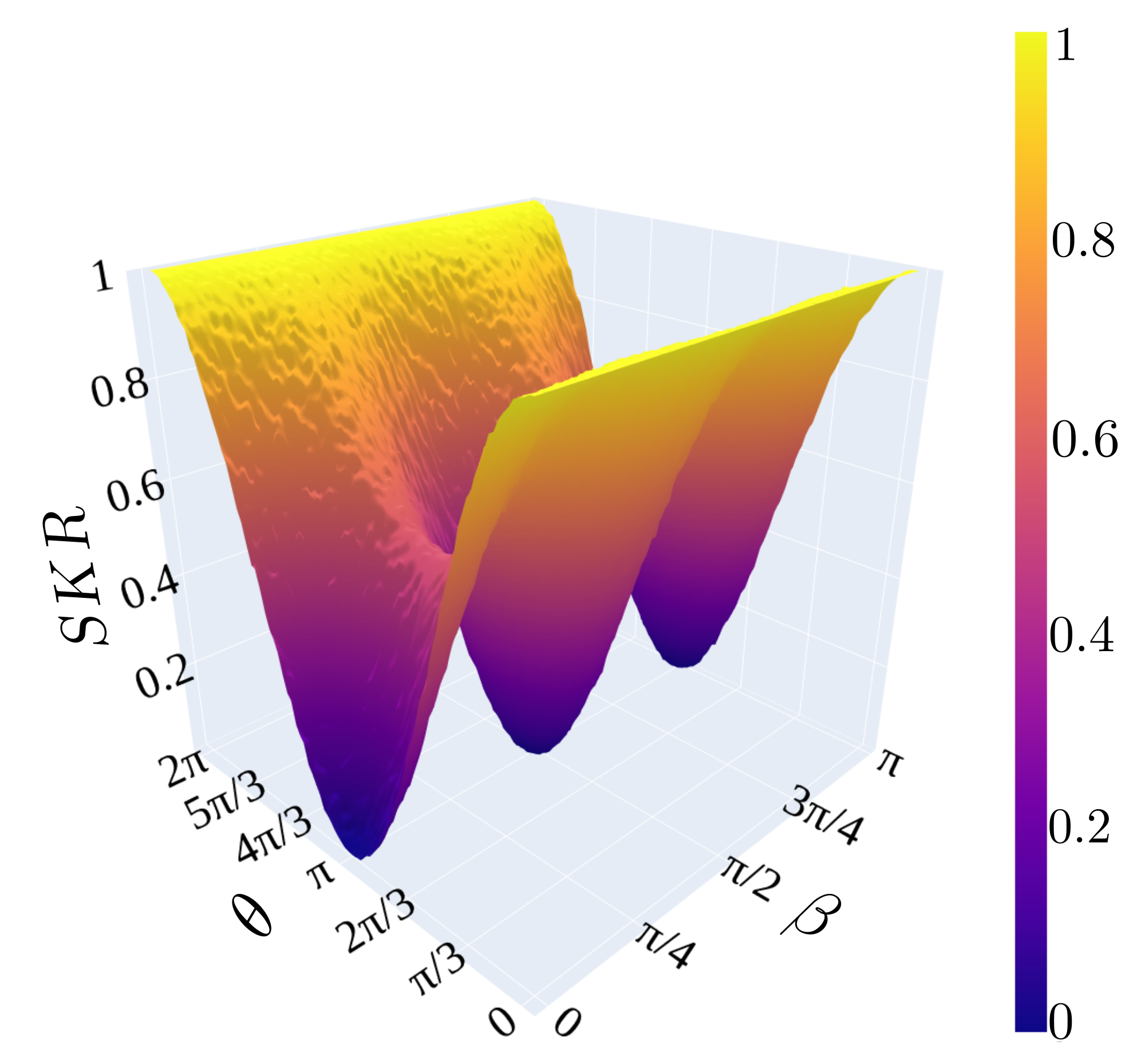
(b) $\alpha=\pi/4$. $R^{2}=0.994$

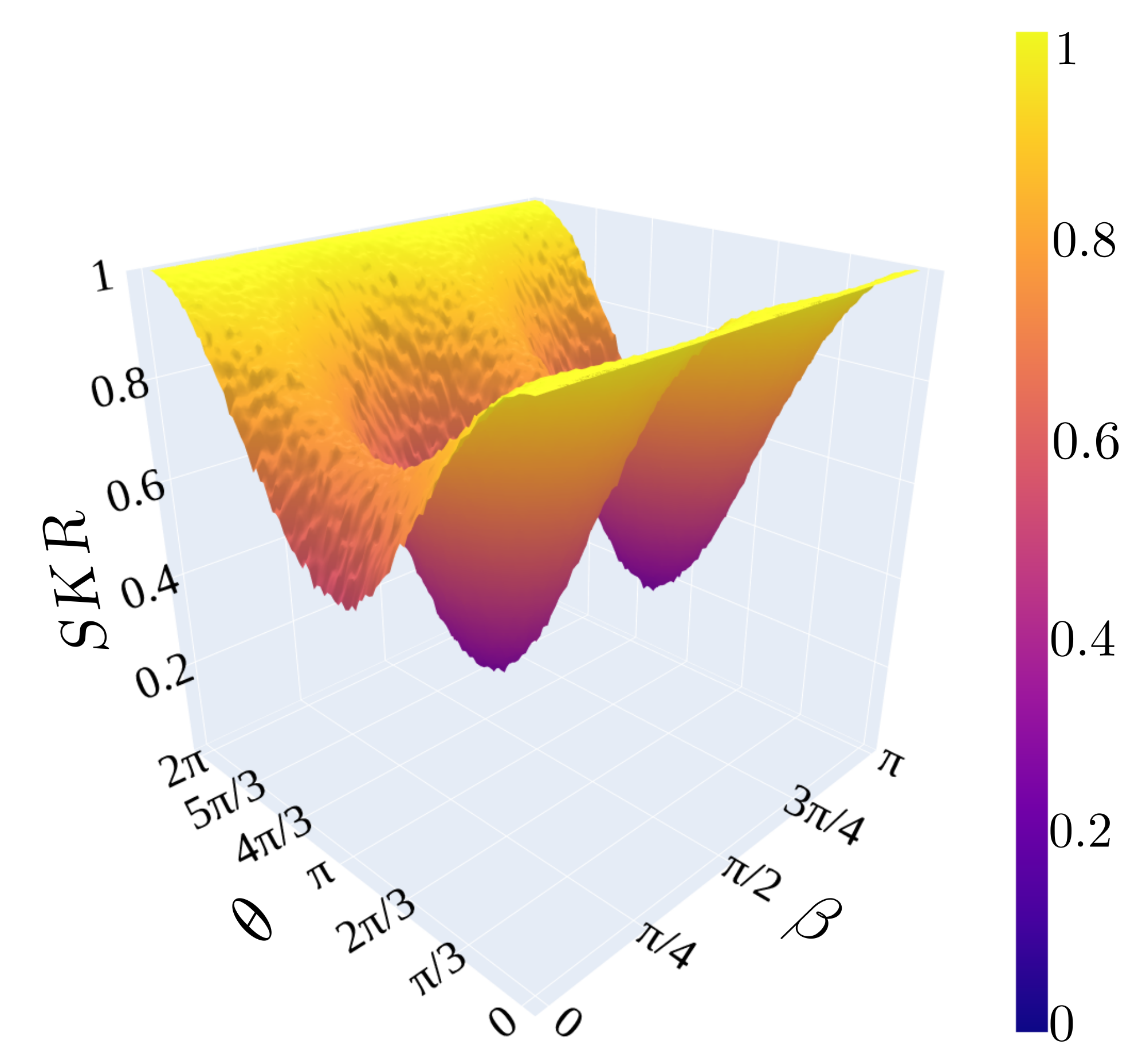
(c) $\alpha=3\pi/8$. $R^{2}=0.997$

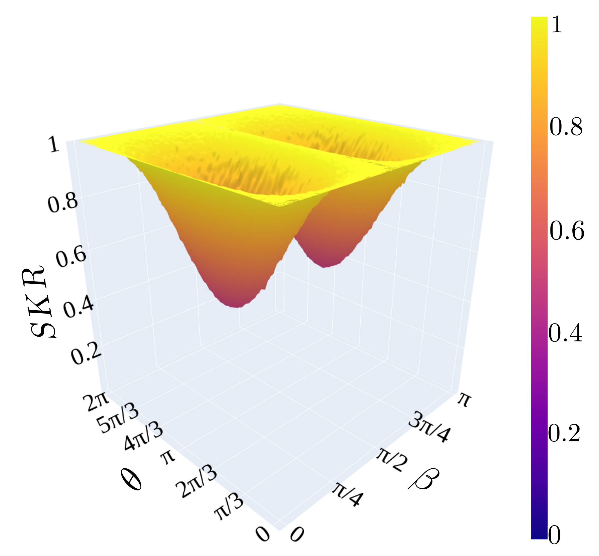
(d) $\alpha=\pi/2$. $R^{2}=0.917$

Figure 4: SKR for $\alpha=\ell\dfrac{\pi}{8}$ with $\ell=1,2,3,4$. The correlation coefficient $R^{2}$ in each panel, indicates the coincidence between the regression of the corresponding data and the analytical expression (equation (8)).

For the simulations, the parameters $\alpha$ and $\beta$ ($\theta_{FSS}$) were varied within the interval $\left[0,\pi\right]$ ($\left[0,2\pi\right]$). Nonetheless, only multiples of $\pi/8$ were considered for $\alpha$.

For each execution of the protocol, associated to a set of $\theta_{\text{FSS}}$, $\alpha$, and $\beta$ values, a total of $5\times 10^{4}$ events (entangled input states) were used to reduce the error margin in the $SKR$. Overall, we run $10^{4}$ executions of the protocol.

Figure 4 shows the quantum computing simulations for $SKR$, obtained for $\alpha=\ell\pi/8$ with $\ell=1,2,3,4$, as functions of $\theta_{FSS}$ and $\beta$.

A correlation index $R^{2}\gtrsim 0.92$ was obtained for all the shown cases, which represents a quite satisfactory match between the computational implementation and the analytical result in equation (8), validating our model.

The surface plots show a strong dependence of $SKR$ on $\theta_{\text{FSS}}$, for most values of $\beta$, presenting the minimum performance in $\theta_{\text{FSS}}=\pi$. The only exceptions to this behavior are observed in the cases $\alpha=n\pi/2$ with $n$ integer, in which $SKR$ is independent on $\theta_{\text{FSS}}$ for $\beta=n\pi/2$. This is a trivial an useless scenario for which both polarizers are along the same direction, and that coincides with the orientation defined by the computational basis. In fact, any case in which $\beta$ is a multiple of $\pi$, independently on the value of $\alpha$, corresponds to a condition under which the protocol cannot be securely applied, because the randomness in the election of basis for measurements would be lost, and interception of Alice’s or Bob’s photons may result in exposition of the key.

It can be seen in figure 4, how $SKR$ oscillates on $\beta$ with a period of $\pi/2$, and that the position and depth of the minima depend on $\alpha$. Transversal cuts at different values of $\beta$ have alike features in the considered interval. It initiates with $SKR=1$, indicating an optimal performance of the protocol. Then, it decays until a minimum at $\theta_{\text{FSS}}=\pi$, where it starts increasing again until recovering ideal operation of the protocol at $\theta_{\text{FSS}}=2\pi$.

There are two scenarios in which the minimum $SKR$ reach extreme values. $\alpha=n\pi/2$ and $\alpha=(2n+1)\pi/4$ ($n=0,1,2,3...$).

In the former case, the minimum $SKR$ value is $0.5$, indicating total randomness in the correlation of Alice’s and Bob’s measurements. In that configuration, the minima are located in $\beta=(2n+1)\pi/4$. Something expected, because orthogonality of the detection polarizers leads to minimum correlation [64].

In the latter case, the lowest value for $SKR$ is $0$, which interestingly implies that in such configuration, for $\theta_{\text{FSS}}=\pi$, the intended correlation in Alice’s and Bob’s measurements, turns into perfect anticorrelation.

We also use the data form the simulations to validate our model. Hence, we calculated the $\left|\left\langle CR\right\rangle\right|$ quantity in terms of $\theta_{\text{FSS}}$ to compare the results with the corresponding derived expression in equation (9).

Figure 5 shows the correspondence between the analytical expression and the points from the simulations for the case $\alpha=\pi/8$ and $\beta=\pi/8$, i.e. the same orientations proposed originally by Ekert to maximize the violation of the Bell’s inequality CHSH. The protocol was executed $10^{3}$ times, with $5\times 10^{4}$ events (entangled input states) per execution. A high correlation between the predicted $CR$ function and the results from the quantum computing implementation was found, with an index of $R^{2}\approx 0.999$.

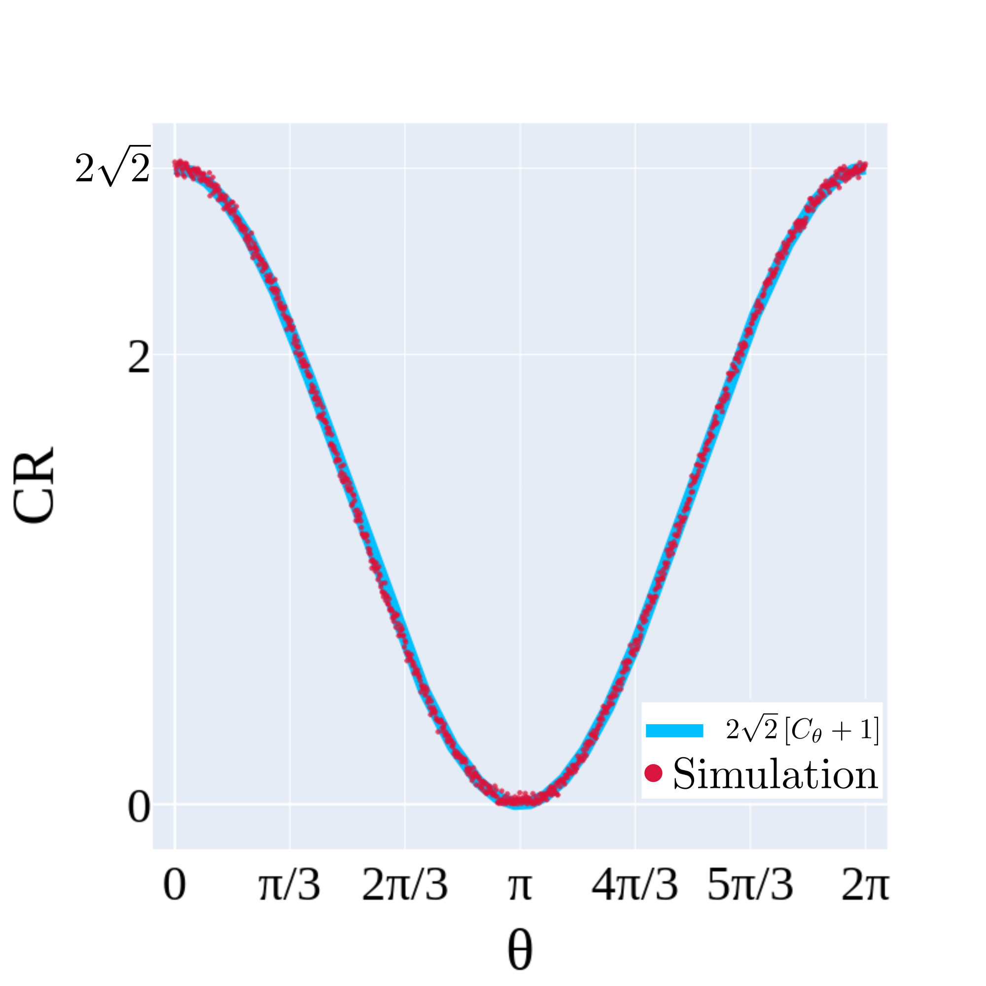
Figure 5: Derived $\left|\left\langle CR\right\rangle\right|$, from equation (9), as a function of $\theta_{\text{FSS}}$ (blue solid line) and the corresponding quantity calculated for 1000 executions with different values of $\theta_{\text{FSS}}$ (red dots). $\alpha=\beta=\pi/8$ were used. The correlation index between the analytical prediction and the simulations is $R^{2}=0.999$.

The oscillations of $CR$ on $\theta_{\text{FSS}}$ imply that computing such a quantity to prove security in the key transmission, may trigger spurious alerts because $CR<2\sqrt{2}$ could happen even in absence of eavesdropping, as long as the FSS in the QD source is not negligible. This suggests that in presence of non-vanishing $S$ for the entanglement source, alternative mechanisms for verifying the security of the transmission should be devised. An option, if the photon leaking rate $LKR$ for transmission and detection is well characterized (in our case it is taken as zero), would be to test

$$SKR+QBER+LKR=1,$$ (13)

which should be fulfilled if no eavesdropping were present.

Summarizing, our analytical and computational results prove that the performance of the QKD protocol E91 depend substantially on the dephasing in the input entangles state. For a wide range of $theta_{\text{FSS}}$ values, such a dephasing strongly diminishes the ability of the protocol to provide a mechanism for transmitting reliable keys.

Besides effective reduction of either the FSS or the exciton lifetime in the QD used to produce the entangled states, a possibility for mitigating the unfavorable effects of the dephasing is to adjust the detection angles in the protocol implementation. According to figure 4, $\alpha$ and $\beta$ could be tuned to rise the minimum $SKR$, extending the range of $theta_{\text{FSS}}$ values along which $QBER$ would remain within the acceptable regime established by the Shannon limit ($<0.11$) [66, 67].

Finally, we would like to remark that although these results were obtained considering the effects of the FSS on the entangled state produced by a QD source, they are applicable in situations where other sources of dephasing can be considered, e.g. recapture, valence band mixing and exciton-spin flipping [56].

VI Conclusions

We studied the performance of the QKD protocol E91 under the effects of dephased polarization-entangled states generated by radiative cascade in a QD source. We also investigated the influence of varying the orientation of the measurement polarizers by parameterizing the directions in which there can be coincidence of the analyzers.

We derived explicit expressions for the performance of the quantum distribution and for the quantity used to carry out the CHSH-type Bell test in the stage of security verification, as functions of the phase of the entangled state and of the varying angles in the protocol realization. Those analytical expressions were satisfactorily validated by multiple simulations from a quantum computing implementation of the protocol, executed in the IBM’s Qiskit Aer simulator.

According to our results, the secret key rate for the transmission is substantially affected by the dephasing in the entangled state. Under some conditions, the value of this rate may be as low as 0.5, which corresponds to a scenario where the protocol becomes completely ineffective.

In turn, the parameter for the Bell test also oscillates on the magnitude of the dephasing, reaching values in which the CHSH inequality is not violated. This may lead to false positives in the stage for detection of eavesdropping.

The observed dependence of the secret key rate on the varying angles of the measurement polarizers, suggest a mechanism to remediate the adverse effects generated on the reliability of the key transmission, by the exciton fine structure splitting of the quantum dot used to produce the entangled states.

These findings provide valuable insight on the standing challenges and potential solutions toward the large scale use of novel sources of entanglement in emerging technologies like quantum communication and quantum cryptography.

———————–

Appendix A Detailed derivations

A.1 Correlation probability computation

We consider a general case in which a pair of entangled photons in a state of the form shown in equation (2), are measured along two arbitrary directions, respectively chosen by Alice and Bob.

The two possible outcome states for one of the photons, after being measured along a basis rotated an angle $\phi$ respect to the default orientations $H$ and $V$, are

$$\left|+_{\phi}\right\rangle =C_{\phi}\left|H\right\rangle+S_{\phi}\left|V\right\rangle,$$ (14)

$$\left|-_{\phi}\right\rangle =-S_{\phi}\left|H\right\rangle+C_{\phi}\left|V\right\rangle.$$ (15)

Consequently, these states are the eigenvectors of a single-photon unitary operator associated to the rotated polarization detector [64]. Such an operator would be given by

$$\begin{split}\widehat{U}\left(\phi\right)=&C_{2\phi}\left|+_{\phi}\right\rangle\left\langle H\right|-S_{2\phi}\left|+_{\phi}\right\rangle\left\langle V\right|+S_{2\phi}\left|-_{\phi}\right\rangle\left\langle H\right|\\ &+C_{2\phi}\left|-_{\phi}\right\rangle\left\langle V\right|.\end{split}$$ (16)

Let’s assume Alice (Bob) sets her (his) analyzer in the direction $\phi_{a}/2$ ($\phi_{b}/2$).

Then we apply the corresponding operators on Alice’s and Bob’s photons to obtain the polarization entangled state written in the basis described in equation (14), namely

$$\begin{split}\left|\psi^{\prime}\right\rangle=\dfrac{1}{\sqrt{2}}\Big{[}&\widehat{U}\left(\phi_{a}/2\right)\otimes\widehat{U}\left(\phi_{b}/2\right)\left|H_{XX}H_{X}\right\rangle+\\ &e^{-i\theta}\widehat{U}\left(\phi_{a}/2\right)\otimes\widehat{U}\left(\phi_{b}/2\right)\left|V_{XX}V_{X}\right\rangle\Big{]}\\ \left|\psi^{\prime}\right\rangle=\dfrac{1}{\sqrt{2}}\Big{[}&\left|+_{\phi_{a}}+_{\phi_{b}}\right\rangle\left(C_{\phi_{a}}C_{\phi_{b}}+e^{-i\theta_{FSS}}S_{\phi_{a}}S_{\phi_{b}}\right)+\\ &\left|-_{\phi_{a}}-_{\phi_{b}}\right\rangle\left(S_{\phi_{a}}S_{\phi_{b}}+e^{-i\theta_{FSS}}C_{\phi_{a}}C_{\phi_{b}}\right)+\\ &\left|+_{\phi_{a}}-_{\phi_{b}}\right\rangle\left(C_{\phi_{a}}S_{\phi_{b}}-e^{-i\theta_{FSS}}S_{\phi_{a}}C_{\phi_{b}}\right)+\\ &\left|-_{\phi_{a}}+_{\phi_{b}}\right\rangle\left(S_{\phi_{a}}C_{\phi_{b}}-e^{-i\theta_{FSS}}C_{\phi_{a}}S_{\phi_{b}}\right)\Big{]}.\end{split}$$ (17)

This expression allows to compute the correlation probabilities $P_{++}$ and $P_{--}$ directly from the superposition coefficients. Because of the symmetry between the square of the projection for $\left|+_{\phi_{a}}+_{\phi_{b}}\right\rangle$ and $\left|+_{\phi_{a}}+_{\phi_{b}}\right\rangle$, we only show the derivation for $P_{++}$, which reads

$$\begin{split}P_{++}&=\Big{|}\langle+_{\phi_{a}}+_{\phi_{b}}|\psi\rangle\Big{|}^{2}\\ &=\dfrac{1}{2}\Big{|}C_{\phi_{a}}C_{\phi_{b}}+e^{-i\theta_{FSS}}S_{\phi_{a}}S_{\phi_{b}}\Big{|}^{2}\\ P_{++}&=\dfrac{1}{2}\left[C_{\phi_{a}}^{2}C_{\phi_{b}}^{2}+S_{\phi_{a}}^{2}S_{\phi_{b}}^{2}+2S_{\phi_{a}}C_{\phi_{a}}S_{\phi_{b}}C_{\phi_{b}}C_{\theta_{FSS}}\right].\end{split}$$ (18)

The data used to generate the key are those in which Alice’s and Bob’s measurement directions coincide. Hence, we take the case $\phi_{a}=\phi_{b}=\phi$, so that

$$P_{++}=\dfrac{1}{2}\left[C_{\phi}^{4}+S_{\phi}^{4}+2S_{\phi}^{2}C_{\phi}^{2}C_{\theta_{FSS}}\right],$$ (19)

which corresponds to equation (5) in the main text.

To compute the probability of anticorrelation, we can proceed analogously, to obtain $P_{\pm\mp}$ from the superposition coefficients of the states $\left|+_{\phi_{a}}-_{\phi_{b}}\right\rangle$ and $\left|-_{\phi_{a}}+_{\phi_{b}}\right\rangle$.

$$\begin{split}P_{+-}&=\Big{|}\langle\pm_{\phi_{a}}\mp_{\phi_{b}}|\psi\rangle\Big{|}^{2}\\ &=\dfrac{1}{2}\Big{|}C_{\phi_{a}}S_{\phi_{b}}-e^{-i\theta_{FSS}}S_{\phi_{a}}C_{\phi_{b}}\Big{|}^{2}\\ P_{+-}&=\dfrac{1}{2}\left[C_{\phi_{a}}^{2}S_{\phi_{b}}^{2}+S_{\phi_{a}}^{2}C_{\phi_{b}}^{2}-2S_{\phi_{a}}C_{\phi_{a}}S_{\phi_{b}}C_{\phi_{b}}C_{\theta_{FSS}}\right].\end{split}$$ (20)

A.2 Derivation of the angle-dependent $CR$ quantity

To compute $CR$ we use the correlation coefficients $E_{ab}=E(\phi_{a},\phi_{b},\theta_{FSS})$, where $\phi_{a}$ ($\phi_{b}$) stands for the measurement direction selected by Alice (Bob). Such coefficients are calculated in terms of the corresponding correlation and anticorrelation probabilities [17]. For those coefficients, we obtain

$$\begin{split}E_{ab}=&P_{++}+P_{--}-P_{+-}-P_{-+}\\ E_{ab}=&C_{\phi_{a}}^{2}C_{\phi_{b}}^{2}+S_{\phi_{a}}^{2}S_{\phi_{b}}^{2}+2S_{\phi_{a}}C_{\phi_{a}}S_{\phi_{b}}C_{\phi_{b}}C_{\theta_{FSS}}\\ -&C_{\phi_{a}}^{2}S_{\phi_{b}}^{2}-S_{\phi_{a}}^{2}C_{\phi_{b}}^{2}+2S_{\phi_{a}}C_{\phi_{a}}S_{\phi_{b}}C_{\phi_{b}}C_{\theta_{FSS}}\\ E_{ab}=&C_{\phi_{a}}^{2}\left[C_{\phi_{b}}^{2}-S_{\phi_{b}}^{2}\right]-S_{\phi_{a}}^{2}\left[C_{\phi_{b}}^{2}-S_{\phi_{b}}^{2}\right]\\ +&4S_{\phi_{a}}C_{\phi_{a}}S_{\phi_{b}}C_{\phi_{b}}C_{\theta_{FSS}}\\ E_{ab}=&\left[C_{\phi_{a}}^{2}-S_{\phi_{a}}^{2}\right]C_{2\phi_{b}}+S_{2\phi_{a}}S_{2\phi_{b}}C_{\theta_{FSS}}\\ E_{ab}=&C_{2\phi_{a}}C_{2\phi_{b}}+S_{2\phi_{a}}S_{2\phi_{b}}C_{\theta_{FSS}}\end{split}$$ (21)

Thus, this quantity that allows to test the CHSH inequality, is given by

$$\begin{split}CR=&E_{01}+E_{23}-E_{03}+E_{21}\\ CR=&C_{2\phi_{0}}C_{2\phi_{1}}+S_{2\phi_{0}}S_{2\phi_{1}}C_{\theta_{FSS}}\\ +&C_{2\phi_{2}}C_{2\phi_{3}}+S_{2\phi_{2}}S_{2\phi_{3}}C_{\theta_{FSS}}\\ -&C_{2\phi_{0}}C_{2\phi_{3}}-S_{2\phi_{0}}S_{2\phi_{3}}C_{\theta_{FSS}}\\ +&C_{2\phi_{2}}C_{2\phi_{1}}+S_{2\phi_{2}}S_{2\phi_{1}}C_{\theta_{FSS}}\\ CR=&C_{\theta_{FSS}}\Big{[}S_{2\phi_{0}}\left(S_{2\alpha}-S_{2\phi_{3}}\right)+S_{2(\alpha+\beta)}\left(S_{2\phi_{3}}+S_{2\alpha}\right)\Big{]}\\ +&C_{2\phi_{0}}\left(C_{2\alpha}-C_{2\phi_{3}}\right)+C_{2(\alpha+\beta)}\left(C_{2\phi_{3}}+C_{2\alpha}\right).\end{split}$$ (22)

Taken the particular directions $\phi_{0}=0$ and $\phi_{3}=3\pi/8$ (optical implementation of the original protocol), it turns into

$$\begin{split}CR=&C_{\theta_{FSS}}S_{2(\alpha+\beta)}\left[\dfrac{1}{\sqrt{2}}+S_{2\alpha}\right]+C_{2(\alpha+\beta)}\left[C_{2\alpha}-\dfrac{1}{\sqrt{2}}\right]\\ +&C_{2\alpha}+\dfrac{1}{\sqrt{2}},\end{split}$$ (23)

which corresponds to equation (9) in the main text.

References

- Bennett et al. [1983] C. H. Bennett, G. Brassard, S. Breidbart, and S. Wiesner, in Advances in cryptology: Proceedings of Crypto 82 (Springer, 1983) pp. 267–275.
- Ekert [1991a] A. K. Ekert, Quantum Measurements in Optics , 413 (1991a).
- Nielsen and Chuang [2010] M. A. Nielsen and I. L. Chuang, Quantum computation and quantum information (Cambridge university press, 2010).
- Ilic [2007] N. Ilic, Journal of Phy334 1, 22 (2007).
- Bennett et al. [1992] C. H. Bennett, F. Bessette, G. Brassard, L. Salvail, and J. Smolin, Journal of cryptology 5, 3 (1992).
- Ekert et al. [1992] A. K. Ekert, J. G. Rarity, P. R. Tapster, and G. M. Palma, Physical Review Letters 69, 1293 (1992).
- Peng et al. [2007] C.-Z. Peng, J. Zhang, D. Yang, W.-B. Gao, H.-X. Ma, H. Yin, H.-P. Zeng, T. Yang, X.-B. Wang, and J.-W. Pan, Physical review letters 98, 010505 (2007).
- Yin et al. [2016] H.-L. Yin, T.-Y. Chen, Z.-W. Yu, H. Liu, L.-X. You, Y.-H. Zhou, S.-J. Chen, Y. Mao, M.-Q. Huang, W.-J. Zhang, et al., Physical review letters 117, 190501 (2016).
- Wengerowsky et al. [2018] S. Wengerowsky, S. K. Joshi, F. Steinlechner, H. Hübel, and R. Ursin, Nature 564, 225 (2018).
- Yin et al. [2020] J. Yin, Y.-H. Li, S.-K. Liao, M. Yang, Y. Cao, L. Zhang, J.-G. Ren, W.-Q. Cai, W.-Y. Liu, S.-L. Li, et al., Nature 582, 501 (2020).
- Wang et al. [2019] H. Wang, H. Hu, T.-H. Chung, J. Qin, X. Yang, J.-P. Li, R.-Z. Liu, H.-S. Zhong, Y.-M. He, X. Ding, et al., Physical review letters 122, 113602 (2019).
- Meng et al. [2024] Y. Meng, M. L. Chan, R. B. Nielsen, M. H. Appel, Z. Liu, Y. Wang, N. Bart, A. D. Wieck, A. Ludwig, L. Midolo, et al., Nature Communications 15, 7774 (2024).
- Chen et al. [2024] C. Chen, J.-Y. Yan, H.-G. Babin, J. Wang, X. Xu, X. Lin, Q. Yu, W. Fang, R.-Z. Liu, Y.-H. Huo, et al., Nature Communications 15, 5792 (2024).
- Weissflog et al. [2024] M. A. Weissflog, A. Fedotova, Y. Tang, E. A. Santos, B. Laudert, S. Shinde, F. Abtahi, M. Afsharnia, I. Pérez Pérez, S. Ritter, et al., Nature Communications 15, 7600 (2024).
- Einstein et al. [1935] A. Einstein, B. Podolsky, and N. Rosen, Physical review 47, 777 (1935).
- Bell [1964] J. S. Bell, Physics Physique Fizika 1, 195 (1964).
- Clauser et al. [1969] J. F. Clauser, M. A. Horne, A. Shimony, and R. A. Holt, Physical review letters 23, 880 (1969).
- Aspect et al. [1981] A. Aspect, P. Grangier, and G. Roger, Physical review letters 47, 460 (1981).
- Aspect et al. [1982] A. Aspect, P. Grangier, and G. Roger, Physical review letters 49, 91 (1982).
- Tittel et al. [1998] W. Tittel, J. Brendel, H. Zbinden, and N. Gisin, Physical review letters 81, 3563 (1998).
- Fujiwara et al. [2014] M. Fujiwara, K.-i. Yoshino, Y. Nambu, T. Yamashita, S. Miki, H. Terai, Z. Wang, M. Toyoshima, A. Tomita, and M. Sasaki, Optics express 22, 13616 (2014).
- Ekert [1991b] A. K. Ekert, Phys. Rev. Lett. 67, 661 (1991b).
- Wang et al. [2021] Q. Wang, Y. Zheng, C. Zhai, X. Li, Q. Gong, and J. Wang, Journal of Semiconductors 42, 091901 (2021).
- Ling et al. [2008] A. Ling, M. P. Peloso, I. Marcikic, V. Scarani, A. Lamas-Linares, and C. Kurtsiefer, Physical Review A—Atomic, Molecular, and Optical Physics 78, 020301 (2008).
- Fujiwara et al. [2009] M. Fujiwara, M. Toyoshima, M. Sasaki, K. Yoshino, Y. Nambu, and A. Tomita, Applied Physics Letters 95 (2009).
- Dzurnak et al. [2015] B. Dzurnak, R. Stevenson, J. Nilsson, J. Dynes, Z. Yuan, J. Skiba-Szymanska, I. Farrer, D. Ritchie, and A. Shields, Applied Physics Letters 107 (2015).
- Basso Basset et al. [2021] F. Basso Basset, M. Valeri, E. Roccia, V. Muredda, D. Poderini, J. Neuwirth, N. Spagnolo, M. B. Rota, G. Carvacho, F. Sciarrino, et al., Science advances 7, eabe6379 (2021).
- Tittel et al. [2001] W. Tittel, H. Zbinden, and N. Gisin, Physical Review A 63, 042301 (2001).
- Benson et al. [2000] O. Benson, C. Santori, M. Pelton, and Y. Yamamoto, Physical review letters 84, 2513 (2000).
- Yin et al. [2017] J. Yin, Y. Cao, Y.-H. Li, S.-K. Liao, L. Zhang, J.-G. Ren, W.-Q. Cai, W.-Y. Liu, B. Li, H. Dai, et al., Science 356, 1140 (2017).
- Morrison et al. [2023] C. L. Morrison, R. G. Pousa, F. Graffitti, Z. X. Koong, P. Barrow, N. G. Stoltz, D. Bouwmeester, J. Jeffers, D. K. Oi, B. D. Gerardot, et al., Nature Communications 14, 3573 (2023).
- Yu et al. [2023] Y. Yu, S. Liu, C.-M. Lee, P. Michler, S. Reitzenstein, K. Srinivasan, E. Waks, and J. Liu, Nature Nanotechnology 18, 1389 (2023).
- Zahidy et al. [2024] M. Zahidy, M. T. Mikkelsen, R. Müller, B. Da Lio, M. Krehbiel, Y. Wang, N. Bart, A. D. Wieck, A. Ludwig, M. Galili, et al., npj Quantum Information 10, 2 (2024).
- Miloshevsky et al. [2024] A. Miloshevsky, L. M. Cohen, K. V. Myilswamy, M. Alshowkan, S. Fatema, H.-H. Lu, A. M. Weiner, and J. M. Lukens, Optica Quantum 2, 254 (2024).
- Winik et al. [2017] R. Winik, D. Cogan, Y. Don, I. Schwartz, L. Gantz, E. Schmidgall, N. Livneh, R. Rapaport, E. Buks, and D. Gershoni, Physical Review B 95, 235435 (2017).
- Ramírez et al. [2019] H. Y. Ramírez, Y.-L. Chou, and S.-J. Cheng, Scientific Reports 9, 1547 (2019).
- Díaz-Ramírez et al. [2023] J. D. Díaz-Ramírez, S.-Y. Huang, B.-L. Cheng, P.-Y. Lo, S.-J. Cheng, and H. Y. Ramírez-Gómez, Condensed Matter 8, 10.3390/condmat8030084 (2023).
- Pennacchietti et al. [2024] M. Pennacchietti, B. Cunard, S. Nahar, M. Zeeshan, S. Gangopadhyay, P. J. Poole, D. Dalacu, A. Fognini, K. D. Jöns, V. Zwiller, et al., Communications Physics 7, 62 (2024).
- Naik et al. [2000] D. Naik, C. Peterson, A. White, A. Berglund, and P. Kwiat, Physical Review Letters 84, 4733 (2000).
- Chang et al. [2020] C. S. Chang, C. Sabín, P. Forn-Díaz, F. Quijandría, A. Vadiraj, I. Nsanzineza, G. Johansson, and C. Wilson, Physical Review X 10, 011011 (2020).
- Hong and Mandel [1985] C. Hong and L. Mandel, Physical Review A 31, 2409 (1985).
- Guilbert and Gauthier [2014] H. E. Guilbert and D. J. Gauthier, IEEE Journal of Selected Topics in Quantum Electronics 21, 215 (2014).
- Müller et al. [2014] M. Müller, S. Bounouar, K. D. Jöns, M. Glässl, and P. Michler, Nature Photonics 8, 224 (2014).
- Couteau [2018] C. Couteau, Contemporary Physics 59, 291 (2018).
- Huber et al. [2018a] D. Huber, M. Reindl, S. F. Covre da Silva, C. Schimpf, J. Martín-Sánchez, H. Huang, G. Piredda, J. Edlinger, A. Rastelli, and R. Trotta, Physical review letters 121, 033902 (2018a).
- Liu et al. [2019] J. Liu, R. Su, Y. Wei, B. Yao, S. F. C. d. Silva, Y. Yu, J. Iles-Smith, K. Srinivasan, A. Rastelli, J. Li, et al., Nature nanotechnology 14, 586 (2019).
- Vajner et al. [2024] D. A. Vajner, P. Holewa, E. Zieba-Ostój, M. Wasiluk, M. von Helversen, A. Sakanas, A. Huck, K. Yvind, N. Gregersen, A. Musial, et al., ACS photonics 11, 339 (2024).
- Young et al. [2009] R. Young, R. Stevenson, A. Hudson, C. Nicoll, D. Ritchie, and A. Shields, Physical review letters 102, 030406 (2009).
- Ozfidan et al. [2015] I. Ozfidan, M. Korkusinski, and P. Hawrylak, Physical Review B 91, 115314 (2015).
- Hernández-Borda et al. [2023] A. F. Hernández-Borda, M. P. Rojas-Sepúlveda, and H. Y. Ramírez-Gómez, Condensed Matter 8, 90 (2023).
- Bauch et al. [2024] D. Bauch, D. Siebert, K. D. Jöns, J. Förstner, and S. Schumacher, Advanced Quantum Technologies 7, 2300142 (2024).
- Ramirez et al. [2010a] H. Y. Ramirez, C.-H. Lin, W. T. You, S.-Y. Huang, W.-H. Chang, S.-D. Lin, and S.-J. Cheng, Physica E: Low-dimensional Systems and Nanostructures 42, 1155 (2010a).
- Ramirez et al. [2010b] H. Y. Ramirez, C. H. Lin, C. C. Chao, Y. Hsu, W. T. You, S. Y. Huang, Y. T. Chen, H. C. Tseng, W. H. Chang, S. D. Lin, and S. J. Cheng, Phys. Rev. B 81, 245324 (2010b).
- Fognini et al. [2019] A. Fognini, A. Ahmadi, M. Zeeshan, J. Fokkens, S. Gibson, N. Sherlekar, S. Daley, D. Dalacu, P. Poole, K. Jons, et al., ACS Photonics 6, 1656 (2019).
- Kuroda et al. [2013] T. Kuroda, T. Mano, N. Ha, H. Nakajima, H. Kumano, B. Urbaszek, M. Jo, M. Abbarchi, Y. Sakuma, K. Sakoda, et al., Physical Review B 88, 041306 (2013).
- Huber et al. [2018b] D. Huber, M. Reindl, J. Aberl, A. Rastelli, and R. Trotta, Journal of Optics 20, 073002 (2018b).
- Ramirez et al. [2009] H. Y. Ramirez, S.-J. Cheng, and C.-P. Chang, physica status solidi (b) 246, 837 (2009).
- Ramírez and Cheng [2010] H. Y. Ramírez and S.-J. Cheng, Phys. Rev. Lett. 104, 206402 (2010).
- De Greve et al. [2011] K. De Greve, P. L. McMahon, D. Press, T. D. Ladd, D. Bisping, C. Schneider, M. Kamp, L. Worschech, S. Höfling, A. Forchel, and Y. Yamamoto, Nature Physics 7, 872 (2011).
- Seidelmann et al. [2022] T. Seidelmann, C. Schimpf, T. K. Bracht, M. Cosacchi, A. Vagov, A. Rastelli, D. E. Reiter, and V. M. Axt, Phys. Rev. Lett. 129, 193604 (2022).
- Trotta et al. [2015] R. Trotta, J. Martín-Sánchez, I. Daruka, C. Ortix, and A. Rastelli, Physical review letters 114, 150502 (2015).
- Muller et al. [2009] A. Muller, W. Fang, J. Lawall, and G. S. Solomon, Physical review letters 103, 217402 (2009).
- Dusanowski et al. [2022] Ł. Dusanowski, C. Gustin, S. Hughes, C. Schneider, and S. Höfling, Nano Letters 22, 3562 (2022).
- Grynberg et al. [2010] G. Grynberg, A. Aspect, and C. Fabre, Introduction to quantum optics: from the semi-classical approach to quantized light (Cambridge university press, 2010).
- Javadi-Abhari et al. [2024] A. Javadi-Abhari, M. Treinish, K. Krsulich, C. J. Wood, J. Lishman, J. Gacon, S. Martiel, P. D. Nation, L. S. Bishop, A. W. Cross, B. R. Johnson, and J. M. Gambetta, Quantum computing with Qiskit (2024), arXiv:2405.08810 [quant-ph] .
- Lütkenhaus [1999] N. Lütkenhaus, Phys. Rev. A 59, 3301 (1999).
- Lizama-Pérez et al. [2021] L. A. Lizama-Pérez, J. M. López R., and E. H. Samperio, Entropy 23, 10.3390/e23020229 (2021).