Beyond Local Sharpness:
Communication-Efficient Global
Sharpness-aware Minimization
for Federated Learning

Abstract

Federated learning (FL) enables collaborative model training with privacy preservation. Data heterogeneity across edge devices (clients) can cause models to converge to sharp minima, negatively impacting generalization and robustness. Recent approaches use client-side sharpness-aware minimization (SAM) to encourage flatter minima, but the discrepancy between local and global loss landscapes often undermines their effectiveness, as optimizing for local sharpness does not ensure global flatness. This work introduces FedGloSS (Federated Global Server-side Sharpness), a novel FL approach that prioritizes the optimization of global sharpness on the server, using SAM. To reduce communication overhead, FedGloSS cleverly approximates sharpness using the previous global gradient, eliminating the need for additional client communication. Our extensive evaluations demonstrate that FedGloSS consistently reaches flatter minima and better performance compared to state-of-the-art FL methods across various federated vision benchmarks.

1 Introduction

Federated Learning (FL) (McMahan et al., 2017) provides a powerful framework to collaboratively train machine learning models on private data distributed across multiple endpoints. Unlike traditional methods, FL enables edge devices (clients), like smartphones or IoT (Internet of Things) hardware, to train a shared model without compromising their sensitive information. This is achieved through communication rounds, where clients independently train on their local data and then exchange updated model parameters with a central server, preserving data privacy. The optimization on the server side relies on pseudo-gradients (Reddi et al., 2021), i.e., the average of the difference between the global model and the client’s update, which serve as an estimate of the true global gradient on the overall dataset. This approach holds immense potential for privacy-sensitive applications, proving its value in areas like healthcare (Liu et al., 2021; Antunes et al., 2022; Rauniyar et al., 2023; Nevrataki et al., 2023), finance (Nevrataki et al., 2023), autonomous driving (Fantauzzo et al., 2022; Shenaj et al., 2023; Miao et al., 2023), IoT (Zhang et al., 2022), and more (Li et al., 2020a; Wen et al., 2023). However, the real-world deployment of FL presents unique challenges stemming from data heterogeneity and communication costs (Li et al., 2020b). Clients gather their data influenced by various factors such as personal habits or geographical locations, leading to inherent differences across devices (Kairouz et al., 2021; Hsu et al., 2020; Shenaj et al., 2023). This results in the global model suffering from degraded performance and slower convergence (Li et al., 2020d; Karimireddy et al., 2020a; b; Caldarola et al., 2022), with instability emerging as client-specific optimization paths diverge from the global one. This phenomenon, known as client drift (Karimireddy et al., 2020b), limits the model’s ability to generalize to the overall underlying distribution.

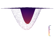
(a) Cifar10
$\alpha=0$

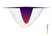
(b) Cifar10
$\alpha=0.05$

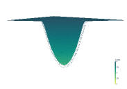
(c) Cifar100
$\alpha=0$

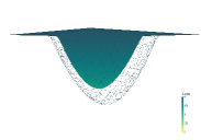
(d) Cifar100
$\alpha=0.5$

Figure 1: Comparison of FedAvg (solid) and FedSam (net) loss landscapes with varying degrees of data heterogeneity ($\alpha$) on the Cifar datasets. FedSam’s effectiveness in converging to global flat minima is highly influenced by the data heterogeneity, where higher heterogeneity ($\alpha\rightarrow 0$) leads to sharper minima, and the complexity of the task, e.g., higher sharpness for the more complex Cifar100. This highlights the importance of optimizing global sharpness. Model: CNN.

While many FL approaches focus on mitigating client drift through client-side regularization (Li et al., 2020c; Acar et al., 2021; Varno et al., 2022), a recent trend leverages the geometry of the loss landscape to improve generalization (Caldarola et al., 2022; Qu et al., 2022; Sun et al., 2023b; Dai et al., 2023; Sun et al., 2023a). These methods build upon the notion that convergence to sharp minima correlates with poor generalization (Hochreiter & Schmidhuber, 1997; Keskar et al., 2017; Jiang et al., 2019). FedSam (Caldarola et al., 2022; Qu et al., 2022) employs Sharpness-aware Minimization (Sam) (Foret et al., 2021) in local training to guide clients toward flatter loss regions, enhancing global performance. This comes at the cost of increased client-side computation, since Sam requires two forward/backward passes for each local optimization step: a gradient ascent step to compute the maximum sharpness and a descent step for sharpness and loss value minimization. Although FedSam and its variants (Sun et al., 2023b; Dai et al., 2023) demonstrated their effectiveness in various settings, they rely solely on local flatness, assuming that minimizing sharpness locally leads to a globally flat minimum. However, in real-world scenarios with significant data heterogeneity, there can be substantial discrepancies between local and global loss landscapes. As a consequence, optimizing for local sharpness does not guarantee the global model will reside in a flat region (Fig. 1). Addressing these limitations, FedSmoo (Sun et al., 2023a) uses the alternating direction method of multipliers (ADMM) (Boyd et al., 2011) to include global sharpness information in Sam’s local training. While this approach reduces the inconsistency between local and global geometries, it increases communication cost by requiring double the bandwidth in each round. This hinders its real-world applicability, as FL relies on minimizing communication overhead (i.e., both message size and exchange frequency) to avoid network congestion and account for potential connection failures, that are common in practical deployments.

Given the limitations of existing methods, achieving convergence to global flat minima while maintaining communication efficiency in heterogeneous FL remains a critical challenge. To address this, we propose FedGloSS (Federated Global Server-side Sharpness) that directly optimizes global sharpness by using Sam on the server side, avoiding additional exchanges over the network. Such adaptation is not straightforward, as Sam would require dual exchanges with each client set per round to solve its optimization problem. Instead, FedGloSS approximates the sharpness measure using available previous pseudo-gradients. As a result, FedGloSS facilitates faster training and keeps communication efficiency. To summarize, our core contributions are the following:

• Empirical proof of local-global discrepancies: we provide the first empirical evidence showing the limitations of approaches that focus solely on local sharpness. Our analysis highlights the inconsistency between local and global loss geometries even when using sharpness-aware approaches like FedSam, demonstrating that local flatness does not necessarily ensure a flat global minimum. While reaching flat global solutions in simpler problems, we show that their effectiveness diminishes as data complexity and heterogeneity increase (Fig. 1).

• To bridge this gap and motivated by communication efficiency, our FedGloSS algorithm directly optimizes for global sharpness on the server using Sam, reducing the communication overhead and the clients’ computational costs compared to previous works. FedGloSS consistently achieves flatter minima and outperforms state-of-the-art methods across various vision benchmarks.

• We show the importance of aligning global and local solutions and illustrate how Sam, especially on the server side, enables effective ADMM use in FL. While typically ADMM-based methods suffer from parameter explosion Varno et al. (2022), we show that by targeting flat minima, Sam encourages smaller gradient steps and minimal weight updates, leading to a significantly more stable algorithm.

2 Related works

Federated framework.

In the last few years, Federated Learning (FL) (McMahan et al., 2017) garnered significant attention from both the machine learning and computer vision communities. While the former has primarily focused on optimizing FL algorithms and guaranteeing their convergence (Li et al., 2020d; Acar et al., 2021; Reddi et al., 2021), the latter has explored its applications in real-world settings, spanning diverse domains like autonomous driving (Fantauzzo et al., 2022; Shenaj et al., 2023; Miao et al., 2023) and healthcare (Liu et al., 2021). The key appeal of FL lies in its ability to efficiently learn from privacy-protected, distributed data while complying with regulations and leveraging edge resources. Real-world deployments of FL range across both cross-silo and cross-device settings (Kairouz et al., 2021). This work focuses on the latter, with up to millions of individual devices at the network edge, with typically limited data and computational power, and potential unavailability due to battery life or network connectivity issues. User-specific factors like geographical location, capturing devices and daily habits introduce inherent bias and statistical heterogeneity into the local datasets. In this setting, FedGloSS aims to learn a global model that generalizes to the overall data distribution under statistical heterogeneity without increasing communication complexity, unlike other algorithms for local-global consistency in heterogeneous FL.

Flatness search in FL. Recent research has explored the connection between loss landscape geometry and generalization in heterogeneous FL. Studies suggest that convergence to sharp minima might hinder generalization performance (Hochreiter & Schmidhuber, 1997; Keskar et al., 2017; Petzka et al., 2021). Sam (Sharpness-Aware Minimization) (Foret et al., 2021) tackles this issue by guiding the optimization toward flatter regions, seeking minima that exhibit both low loss and low sharpness. FedSam (Caldarola et al., 2022; Qu et al., 2022) deploys Sam in local training, marking the first step toward leveraging loss surface geometry in FL to reduce discrepancies between local and global objectives, ultimately improving the global model’s generalization ability. Following its success, FedSpeed (Sun et al., 2023b) uses perturbed gradients as Sam to reduce local overfitting, FedGamma (Dai et al., 2023) combines the stochastic variance reduction of Scaffold with Sam and Shi et al. (2023) show FedSam’s effectiveness in mitigating the negative effects of differential privacy. However, these approaches rely on local sharpness information, assuming its minimization directly translates to a globally flat minimum. This may not always be true, as we hypothesize discrepancies may exist between the geometries of local and global losses. Optimizing local sharpness alone does not guarantee a server model residing in a flat region of the global loss landscape (Fig. 1). Addressing these limitations, FedSmoo (Sun et al., 2023a) applies ADMM (Boyd et al., 2011) to the sharpness measure to enforce global and local consistency. This adds communication overhead, doubling the message size in each round and hindering its real-world practicality. In contrast, our work focuses on minimizing global sharpness while maintaining communication efficiency. Lastly, building on Stochastic Weight Averaging (Izmailov et al., 2018), other works (Caldarola et al., 2022; 2023) use a window-based average of global models across rounds to reach wider minima. Being agnostic to the underlying optimization algorithm, they remain orthogonal to our approach.

Heterogeneity in FL. The de-facto standard algorithm for FL is FedAvg (McMahan et al., 2017), which updates the global model with a weighted average of the clients’ parameters. However, FedAvg struggles when faced with heterogeneous data distributions, leading to performance degradation and slow convergence due to the local optimization paths diverging from the global one (Karimireddy et al., 2020b). Reddi et al. (2021) shows FedAvg is equivalent to applying Stochastic Gradient Descent (Sgd) (Ruder, 2016) with a unitary learning rate on the server side, using the difference between the initial global model parameters and the clients’ updates as pseudo-gradient, opening the door to alternative optimizers beyond Sgd to improve performance and convergence speed. Building on this intuition, this work proposes Sam (Foret et al., 2021) as a server-side optimizer to enhance generalization by converging toward global flat minima. Since Sam requires two optimization steps per iteration, a direct adaptation to the FL setting would double communication exchanges between clients and server; FedGloSS overcomes this limitation and maintains communication efficiency through the use of the latest pseudo-gradient as sharpness approximation.

Several approaches address client drift by adding regularization during local training. FedProx (Li et al., 2020c) introduces a term to keep local parameters close to the global model, FedDyn (Acar et al., 2021) employs ADMM to align local and global convergence points, AdaBest (Varno et al., 2022) adjusts local updates with an adaptive bias estimate, and Scaffold (Karimireddy et al., 2020b) applies stochastic variance reduction. Momentum-based techniques (Sutskever et al., 2013) are also employed to maintain a consistent global trajectory, either on the server side (e.g., FedAvgM (Hsu et al., 2019)) or by incorporating global information into local training (Karimireddy et al., 2020a; Kim et al., 2022; Gao et al., 2022; Zaccone et al., 2023). Unlike FedDyn, where ADMM can lead to parameter explosion (Varno et al., 2022), our FedGloSS successfully leverages ADMM to align global and local solutions, even under extreme heterogeneity, aided by Sam on server.

Centralized SAM. To avoid doubling client-server exchanges caused by Sam’s two-step process, FedGloSS draws on insights from the literature on Sam in centralized settings. Several strategies have been proposed to minimize computational overhead, including reducing the number of parameters needed to compute the sharpness-aware components (Du et al., 2022a), or approximating them (Liu et al., 2022; Du et al., 2022b; Park et al., 2023). DP-SAT (Park et al., 2023) approximates the ascent step with the gradient from the previous iteration, and SAF (Du et al., 2022b) replaces Sam’s sharpness approximation with the trajectory of weights learned during training. Aiming to the same goal, FedGloSS approximates the sharpness measure with the pseudo-gradient from the previous round on the server side, without incurring in unnecessary exchanges with the clients and effectively guiding the optimization toward globally flat minima.

3 Background

This section introduces the FL problem setting and preliminary notations on Sam (Foret et al., 2021) and FedSam (Caldarola et al., 2022; Qu et al., 2022).

3.1 Problem setting

In FL, a central server communicates with a set of clients $\operatorname{\mathcal{C}}$ for $T$ rounds. The goal is to learn a global model $f(\operatorname{\boldsymbol{w}}):\operatorname{\mathcal{X}}\rightarrow\operatorname{\mathcal{Y}}$ parametrized by $\operatorname{\boldsymbol{w}}\in\mathbb{R}^{d}$, where $\operatorname{\mathcal{X}}$ and $\operatorname{\mathcal{Y}}$ are the input and the output spaces respectively. In image classification, $\operatorname{\mathcal{X}}$ contains the images and $\operatorname{\mathcal{Y}}$ their corresponding labels. Each client $k\in\operatorname{\mathcal{C}}$ has access to a local dataset $\operatorname{\mathcal{D}}_{k}$ of $N_{k}$ pairs $\{(x_{i},y_{i}),x_{i}\in\operatorname{\mathcal{X}},y_{i}\in\operatorname{\mathcal{Y}}\}_{i=1}^{N_{k}}$. In realistic heterogeneous settings, clients usually hold different data distributions and quantity, i.e., $\mathit{D}_{i}\neq\mathit{D}_{j}$ and $N_{i}\neq N_{j}\,\forall i\neq j\in\operatorname{\mathcal{C}}$. The global FL objective is:

$$\min_{\operatorname{\boldsymbol{w}}}\left\{f(\operatorname{\boldsymbol{w}})=\frac{1}{C}\sum_{k\in\operatorname{\mathcal{C}}}f_{k}(\operatorname{\boldsymbol{w}})\right\},f_{k}(\operatorname{\boldsymbol{w}})\triangleq\mathbb{E}f_{k}(\operatorname{\boldsymbol{w}},\xi_{k}),$$ (1)

where $C\triangleq|\operatorname{\mathcal{C}}|$ is the total number of clients, $f_{k}$ is the empirical loss on the $k$-th client (e.g., cross-entropy loss) and $\xi_{k}$ is the data sample randomly drawn from the local data distribution $\mathit{D}_{k}$. The training process is a two-phase optimization approach within each round $t\in[T]$. First, due to potential client unavailability, a subset of selected clients $\operatorname{\mathcal{C}}^{t}\subset\operatorname{\mathcal{C}}$ trains the received global model using their local optimizer ClientOpt (e.g., Sgd, Sam). Then, the server aggregates their updates with a server optimizer, ServerOpt. FedOpt (Reddi et al., 2021) solves Eq. 1 as

$$\Delta^{t}_{\operatorname{\boldsymbol{w}}} \triangleq\sum_{k\in\operatorname{\mathcal{C}}^{t}}\frac{N_{k}}{N}(\operatorname{\boldsymbol{w}}^{t}-\operatorname{\boldsymbol{w}}^{t}_{k})\,\text{ and }$$ (2)

$$\operatorname{\boldsymbol{w}}^{t+1} \leftarrow\operatorname{\boldsymbol{w}}^{t}-\textsc{ServerOpt}(\operatorname{\boldsymbol{w}}^{t},\Delta^{t}_{\operatorname{\boldsymbol{w}}},\eta_{s}),$$ (3)

where $\Delta^{t}_{\operatorname{\boldsymbol{w}}}$ is the global pseudo-gradient at round $t$, $N=\sum_{k\in\operatorname{\mathcal{C}}^{t}}N_{k}$ the total number of images seen during the current round, $\eta_{s}$ the server learning rate, $\operatorname{\boldsymbol{w}}^{t}$ the global model and $\operatorname{\boldsymbol{w}}^{t}_{k}$ the local update resulting from training on client $k$’s data with ClientOpt for $E$ epochs. FedAvg (McMahan et al., 2017) computes $\operatorname{\boldsymbol{w}}^{t+1}$ as $\sum_{k\in\operatorname{\mathcal{C}}^{t}}\nicefrac{{N_{k}}}{{N}}\operatorname{\boldsymbol{w}}^{t}_{k}$, corresponding to one SGD step on the pseudo-gradient $\Delta^{t}_{\operatorname{\boldsymbol{w}}}$ with $\eta_{s}=1$ (Reddi et al., 2021).

3.2 Sharpness-aware Minimization

Sam (Foret et al., 2021) jointly minimizes the loss value and the sharpness of the loss landscape by solving the min-max problem

$$\min_{\operatorname{\boldsymbol{w}}}\left\{F(\operatorname{\boldsymbol{w}})\triangleq\max_{\|\operatorname{\boldsymbol{\epsilon}}\|\leq\rho}f(\operatorname{\boldsymbol{w}}+\operatorname{\boldsymbol{\epsilon}})\right\},$$ (4)

where $\operatorname{\boldsymbol{\epsilon}}$ is the perturbation to estimate the sharpness, $f$ the loss function, $\rho$ the neighborhood size and $\|\cdot\|$ the $\ell_{2}$ norm. Using the first-order Taylor expansion of $f$, Sam efficiently solves the inner maximization as

$$\operatorname*{arg\,max}_{\|\operatorname{\boldsymbol{\epsilon}}\|\leq\rho}f(\operatorname{\boldsymbol{w}})+\operatorname{\boldsymbol{\epsilon}}^{\top}\nabla_{\operatorname{\boldsymbol{w}}}f(\operatorname{\boldsymbol{w}})=\rho\frac{\nabla_{\operatorname{\boldsymbol{w}}}f(\operatorname{\boldsymbol{w}})}{\|\nabla_{\operatorname{\boldsymbol{w}}}f(\operatorname{\boldsymbol{w}})\|}\triangleq\operatorname{\hat{\boldsymbol{\epsilon}}}(\operatorname{\boldsymbol{w}}).$$ (5)

$\operatorname{\hat{\boldsymbol{\epsilon}}}$ is the scaled gradient of the loss w.r.t. the current parameters $\operatorname{\boldsymbol{w}}$. The sharpness-aware gradient is $\nabla_{\operatorname{\boldsymbol{w}}}f(\operatorname{\boldsymbol{w}})|_{\operatorname{\boldsymbol{w}}+\operatorname{\hat{\boldsymbol{\epsilon}}}(\operatorname{\boldsymbol{w}})}$. Eq. 4 is solved with a first gradient ascent step to compute $\operatorname{\hat{\boldsymbol{\epsilon}}}$ and a descent step with the sharpness-aware gradient, updating the model as $\operatorname{\boldsymbol{w}}\leftarrow\operatorname{\boldsymbol{w}}-\eta\nabla_{\operatorname{\boldsymbol{w}}}f(\operatorname{\boldsymbol{w}})|_{\operatorname{\boldsymbol{w}}+\operatorname{\hat{\boldsymbol{\epsilon}}}(\operatorname{\boldsymbol{w}})}$.

3.3 SAM in Federated Learning

FedSam (Caldarola et al., 2022; Qu et al., 2022) aims to improve the clients’ models generalization through convergence to flatter regions by using Sam in the local training. From Eqs. 1 and 4, the global objective becomes $\min_{\operatorname{\boldsymbol{w}}}\left\{f^{\textsc{Sam}}(\operatorname{\boldsymbol{w}})=\nicefrac{{1}}{{C}}\sum_{k\in\operatorname{\mathcal{C}}}f_{k}^{\textsc{Sam}}(\operatorname{\boldsymbol{w}})\right\}$, with $f_{k}^{\textsc{Sam}}(\operatorname{\boldsymbol{w}})\triangleq\max_{\|\operatorname{\boldsymbol{\epsilon}}_{k}\|\leq\rho}f_{k}(\operatorname{\boldsymbol{w}}+\operatorname{\boldsymbol{\epsilon}}_{k})$ with local perturbation $\operatorname{\boldsymbol{\epsilon}}_{k}$. The intuition behind this approach is that the improved local models’ generalization positively reflects on the global model performance. However, by independently applying Eq. 4 in the local optimization, FedSam does not explicitly address global flatness, potentially leading to discrepancies between local and global loss geometries.

4 Local-Global Sharpness Inconsistency

This section empirically investigates the hypothesis that discrepancies between local and global loss landscapes impact FedSam’s performance, using a CNN model on Cifar10 and Cifar100 datasets — further details in Section 6.

Fig. 1 compares the loss surfaces of CNNs trained with FedAvg and FedSam. On the easier Cifar10, FedSam exhibits noticeably flatter minima w.r.t. FedAvg, effectively navigating simpler landscapes. However, their performance difference diminishes with increasing dataset complexity (Cifar100) and heterogeneity ($\alpha\rightarrow 0$). This suggests that larger discrepancies between local and global geometries arise as tasks become more complex and data distributions more diverse.

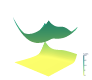
(a) Trained on class sea

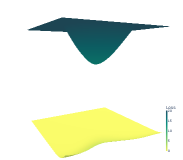
(b) Trained on class snail

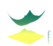
(c) Trained on class skyscraper

Figure 2: Global vs. local perspective on FedSam. Cifar100 $\alpha=0$ @ $20k$ rounds on CNN. Local models trained on one class, tested on the local (bottom landscape) or global dataset (top landscape). Models trained with FedSam present significant differences between local and global behaviors.

To highlight the existing difference between local and global behavior, Fig. 2 investigates the behavior of client models at the end of local training when tested on their own data $\operatorname{\mathcal{D}}_{k}$ (bottom landscape), prior to server-side aggregation, w.r.t. the overall dataset $\operatorname{\mathcal{D}}$ (top landscape). Each plot shows the behavior of one of the randomly selected clients during the last round with FedSam, distinguished by the locally seen class (results for all 5 clients in Appendix B). The inconsistency between local and global behavior can be easily appreciated: locally, each model lands in a flat region; differently, the same model is close to saddle points (Fig. 2(a)) or sharp minima (Figs. 2(b) and 2(c)) in the global landscape. These findings are further corroborated by the Hessian eigenvalues presented in Table 1. FedSam’s local maximum Hessian eigenvalue, denoted by $\lambda_{1,l}$ and computed on each client’s individual dataset, is significantly lower than the global eigenvalue $\lambda_{1,g}$, calculated on the overall dataset, on the more complex Cifar100. This suggests that FedSam effectively achieves local convergence to flatter regions of the loss landscape on individual devices. However, the higher global eigenvalue indicates limitations in reaching a globally flat minimum. The challenge of achieving flat regions under high heterogeneity and the gap between local and global flatness support the introduction of FedGloSS.

Table 1: Maximum Hessian eigenvalues of local models, computed on global ($\lambda_{1,g}$) and local datasets ($\lambda_{1,l}$). Cifar10 and Cifar100, $\alpha=0$. Each client is identified via its local class. The lowest $\lambda_{1,g}$ in bold. FedDyn does not converge on Cifar100 with $\alpha=0$ (Caldarola et al., 2022; Varno et al., 2022), hence the lack of results (✗).

	Local	FedAvg			FedSam			FedDyn			FedDyn + Sam			FedSmoo			FedGloSS
	Class	$\lambda_{1,l}$	$\lambda_{1,g}$		$\lambda_{1,l}$	$\lambda_{1,g}$		$\lambda_{1,l}$	$\lambda_{1,g}$		$\lambda_{1,l}$	$\lambda_{1,g}$		$\lambda_{1,l}$	$\lambda_{1,g}$		$\lambda_{1,l}$	$\lambda_{1,g}$
Cifar10	airplane	9.1	239.1		100.6	36.4		752.5	347.8		199.6	12.0		122.1	26.5		190.1	4.3
	cat	424.2	273.6		28.8	16.5		59.9	242.3		122.0	11.1		82.4	26.9		106.9	3.9
	bird	18.4	237.0		106.4	35.7		894.0	371.2		200.2	12.0		134.2	25.7		200.1	4.1
	airplane	483.5	269.5		103.2	30.6		761.6	348.9		206.9	12.3		122.8	25.2		207.8	4.0
	frog	263.2	259.6		68.1	32.9		528.9	286.0		155.6	11.7		79.3	33.5		84.8	4.1
Cifar100	sea	251.0	224.5		0.1	238.5		✗	✗		✗	✗		33.2	31.4		28.3	19.6
	snail	91.2	267.0		0.2	149.1								331.2	102.2		260.8	40.7
	bear	108.4	215.2		6.7	129.3								428.6	121.0		220.3	49.6
	skyscraper	613.3	300.1		1.3	194.6								143.5	40.2		269.2	22.2
	possum	37.9	259.6		15.3	142.6								455.5	90.9		392.4	39.0

5 FL with Global Server-side Sharpness

FedGloSS (Federated Global Server-side Sharpness) overcomes FedSam’s limitations by efficiently optimizing both global flatness and consistency.

5.1 Rethinking SAM in Federated Learning

Aiming to optimize Sam’s objective (Eq. 4) on the global function, FedGloSS solves $\min_{\operatorname{\boldsymbol{w}}}\left\{\operatorname{\mathcal{F}}(\operatorname{\boldsymbol{w}})=\frac{1}{C}\sum_{k\in\operatorname{\mathcal{C}}}\operatorname{\mathcal{F}}_{k}(\operatorname{\boldsymbol{w}})\right\}$, with $\operatorname{\mathcal{F}}_{k}(\operatorname{\boldsymbol{w}})\triangleq\max_{\|\operatorname{\boldsymbol{\epsilon}}\|\leq\rho}f_{k}(\operatorname{\boldsymbol{w}}+\operatorname{\boldsymbol{\epsilon}})$, where $\operatorname{\boldsymbol{\epsilon}}$ is the global perturbation. Calculating the true $\operatorname{\boldsymbol{\epsilon}}$ value requires the global gradient $\nabla_{\operatorname{\boldsymbol{w}}}f$ (Eq. 5) computed on the entire dataset $\operatorname{\mathcal{D}}\triangleq\cup_{k\in\operatorname{\mathcal{C}}}\operatorname{\mathcal{D}}_{k}$, which is not available in FL due to data privacy and communication constraints. While FedSmoo (Sun et al., 2023a) tackles this issue by using ADMM on the sharpness with the constraint $\operatorname{\boldsymbol{\epsilon}}=\operatorname{\boldsymbol{\epsilon}}_{k}$, it necessitates transmitting $\operatorname{\boldsymbol{\epsilon}}$ alongside the model parameters $\operatorname{\boldsymbol{w}}$ to both clients and server in each round, hindering its practicality in real-world scenarios with limited communication budgets. This observation motivates the question: how to minimize global sharpness while maintaining communication efficiency?

5.1.1 Challenges of Server-side SAM

We address this question by applying Sam on the server side, directly optimizing for global sharpness and eliminating the need to align local sharpness on the clients. The global model has to be updated as $\operatorname{\boldsymbol{w}}^{t+1}\leftarrow\operatorname{\boldsymbol{w}}^{t}-\eta_{s}\nabla_{\operatorname{\boldsymbol{w}}}\operatorname{\mathcal{F}}(\operatorname{\boldsymbol{w}})|_{\operatorname{\boldsymbol{w}}^{t}+\operatorname{\hat{\boldsymbol{\epsilon}}}^{t}(\operatorname{\boldsymbol{w}})}$, where $\operatorname{\hat{\boldsymbol{\epsilon}}}^{t}$ is the global perturbation at each round $t$. However, a key challenge arises: the computation of both $\operatorname{\hat{\boldsymbol{\epsilon}}}^{t}$ and the sharpness-aware gradient necessitates two transmissions with the clients, making its direct application in server-side FL non-trivial. A straightforward solution is to emulate SAM’s double computation step through two communication exchanges $\forall t\in[T]$.

• Step 1: the server sends the global model $\operatorname{\boldsymbol{w}}^{t}$ to a subset $\operatorname{\mathcal{C}}^{t}$ of clients, which update it using their local data. With the resulting pseudo-gradient $\Delta^{t}_{\operatorname{\boldsymbol{w}}}$, $\operatorname{\hat{\boldsymbol{\epsilon}}}^{t}(\operatorname{\boldsymbol{w}})=\rho(\nicefrac{{\Delta^{t}_{\operatorname{\boldsymbol{w}}}}}{{\|\Delta^{t}_{\operatorname{\boldsymbol{w}}}\|}})$ and the perturbed model $\operatorname{\tilde{\boldsymbol{w}}}^{t}=\operatorname{\boldsymbol{w}}^{t}+\operatorname{\hat{\boldsymbol{\epsilon}}}^{t}(\operatorname{\boldsymbol{w}})$.

• Step 2: the server transmits $\operatorname{\tilde{\boldsymbol{w}}}^{t}$ to the same $\operatorname{\mathcal{C}}^{t}$, which compute their update $\operatorname{\tilde{\boldsymbol{w}}}_{k}^{t}\,\forall k$. The resulting global pseudo-gradient $\tilde{\Delta}^{t}_{\operatorname{\boldsymbol{w}}}\triangleq\sum_{k\in\operatorname{\mathcal{C}}^{t}}\nicefrac{{N_{k}}}{{N}}(\operatorname{\tilde{\boldsymbol{w}}}^{t}-\operatorname{\tilde{\boldsymbol{w}}}^{t}_{k})$ is an estimate of $\nabla_{\operatorname{\boldsymbol{w}}}\operatorname{\mathcal{F}}(\operatorname{\boldsymbol{w}})|_{\operatorname{\boldsymbol{w}}^{t}+\operatorname{\hat{\boldsymbol{\epsilon}}}^{t}(\operatorname{\boldsymbol{w}})}$.

This two-step approach, referred to as NaiveFedGloSS, is conceptually simple but suffers from communication inefficiency, doubling the communication cost w.r.t. FedAvg, while requiring the same set of clients $\operatorname{\mathcal{C}}^{t}$ to remain active for two consecutive exchanges. This may be unrealistic in real-world settings often characterized by network failures. These limitations highlight the need for an efficient alternative that accounts for practical real-world FL factors.

5.2 FedGloSS

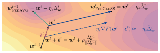
Figure 3: Illustration of FedGloSS. The model $\operatorname{\boldsymbol{w}}^{t}$ is perturbed using $\tilde{\Delta}_{\operatorname{\boldsymbol{w}}}^{t-1}$. The sharpness-aware direction (dashed) is used to compute $\operatorname{\boldsymbol{w}}^{t+1}$ (solid), which lands in a flat region. Compared to FedAvg.

Table 2: Overview of FL methods using Sam. Differently from previous works, FedGloSS uses Sam as server optimizer and allows any local optimizer.

Method	ServerOpt	ClientOpt	Global	Communication	Local Computation
			Flatness	Cost	Cost
FedSam (Caldarola et al., 2022; Qu et al., 2022)	Sgd	Sam	✗	$1\times$	$2\times$
FedDyn (Acar et al., 2021) + Sam	Sgd	Sam	✗	$1\times$	$2\times$
FedSpeed (Sun et al., 2023b)	Sgd	Similar to Sam	✗	$1\times$	$2\times$
FedGamma (Dai et al., 2023)	Sgd	Sam	✓	$2\times$	$2\times$
FedSmoo (Sun et al., 2023a)	Sgd	Sam	✓	$2\times$	$2\times$
FedGloSS	Sam	Any optimizer	✓	$1\times$	$1\times$ or $2\times$

To overcome the challenges posed by NaiveFedGloSS, following (Park et al., 2023), FedGloSS estimates $\operatorname{\hat{\boldsymbol{\epsilon}}}^{t}$ using the perturbed global pseudo-gradient from the previous round $\tilde{\Delta}^{t-1}_{\operatorname{\boldsymbol{w}}}$ at each round $t$. This approach leverages available information without incurring extra communications and avoiding unnecessary computations. Intuitively, the use of the previous pseudo-gradient to minimize the sharpness allows FedGloSS to access information on the global loss landscape geometry, thus guiding the global optimization towards flatter minima. From Eqs. 5 and 3, FedGloSS updates the global model $\operatorname{\boldsymbol{w}}^{t}$ as

$${\footnotesize1}⃝ \,{\color[rgb]{0.62,0.31,0.56}\operatorname{\tilde{\boldsymbol{\epsilon}}}^{t}(\operatorname{\boldsymbol{w}})}\triangleq\rho\frac{\tilde{\Delta}^{t-1}_{\operatorname{\boldsymbol{w}}}}{\|\tilde{\Delta}^{t-1}_{\operatorname{\boldsymbol{w}}}\|}$$

$${\footnotesize2}⃝ \,\operatorname{\tilde{\boldsymbol{w}}}^{t}\leftarrow\operatorname{\boldsymbol{w}}^{t}{\color[rgb]{0.62,0.31,0.56}+\operatorname{\tilde{\boldsymbol{\epsilon}}}^{t}(\operatorname{\boldsymbol{w}})}$$

$${\footnotesize3}⃝ \,\text{Obtain $\operatorname{\tilde{\boldsymbol{w}}}^{t}_{k}$ from clients and }\tilde{\Delta}^{t}_{\operatorname{\boldsymbol{w}}}=\sum_{k\in\operatorname{\mathcal{C}}^{t}}\frac{N_{k}}{N}(\operatorname{\tilde{\boldsymbol{w}}}^{t}-\operatorname{\tilde{\boldsymbol{w}}}^{t}_{k})$$

$${\footnotesize4}⃝ \operatorname{\boldsymbol{w}}^{t+1}\leftarrow\operatorname{\boldsymbol{w}}^{t}{\color[rgb]{0,0.45,0.75}-{\textsc{FedGloSS}}(\operatorname{\boldsymbol{w}}^{t},\tilde{\Delta}^{t}_{\operatorname{\boldsymbol{w}}},\eta_{s})}=\operatorname{\boldsymbol{w}}^{t}{\color[rgb]{0,0.45,0.75}-\eta_{s}\tilde{\Delta}^{t}_{\operatorname{\boldsymbol{w}}}},$$

where with a slight abuse of notation ServerOpt from Eq. 3 is substituted with the server-side strategy proposed by FedGloSS. The notation follows the colors of Fig. 3, which depicts our approach. Notably, as summarized in Table 2, FedGloSS enables Sam on the server side while allowing any ClientOpt for local training, with computational costs varying based on the chosen optimizer. This differs from previous methods constrained to the more computationally expensive Sam. In addition, differently from FedSmoo, FedGloSS maintains FedAvg’s communication complexity while optimizing for global flatness.

5.2.1 Promoting global consistency with ADMM

The difference in using the approximation $\operatorname{\tilde{\boldsymbol{\epsilon}}}^{t}$ (FedGloSS) and the true $\operatorname{\hat{\boldsymbol{\epsilon}}}^{t}$ (NaiveFedGloSS) is

$$\delta_{\epsilon}^{t}\triangleq\|\operatorname{\tilde{\boldsymbol{\epsilon}}}^{t}(\operatorname{\boldsymbol{w}})-\operatorname{\hat{\boldsymbol{\epsilon}}}^{t}(\operatorname{\boldsymbol{w}})\|=\rho\left\|\frac{\tilde{\Delta}^{t-1}_{\operatorname{\boldsymbol{w}}}}{\|\tilde{\Delta}^{t-1}_{\operatorname{\boldsymbol{w}}}\|}-\frac{{\Delta}^{t}_{\operatorname{\boldsymbol{w}}}}{\|{\Delta}^{t}_{\operatorname{\boldsymbol{w}}}\|}\right\|,$$ (6)

where $\tilde{\Delta}^{t-1}_{\operatorname{\boldsymbol{w}}}$ is computed using the updates of the clients in $\operatorname{\mathcal{C}}^{t-1}$ and $\tilde{\Delta}^{t}_{\operatorname{\boldsymbol{w}}}$ with $\operatorname{\mathcal{C}}^{t}$. Eq. 6 suggests $\delta_{\epsilon}^{t}$ is minimized when $\tilde{\Delta}^{t-1}_{\operatorname{\boldsymbol{w}}}$ and $\tilde{\Delta}^{t}_{\operatorname{\boldsymbol{w}}}$ are aligned. However, in real-world heterogeneous FL, i) to due clients’ unavailability, only a subset of them participates in training at each round, with $\operatorname{\mathcal{C}}^{t}$ likely differing from $\operatorname{\mathcal{C}}^{t-1}$, and ii) clients hold different data distributions, i.e., local optimization paths likely converge towards different local minima, leading to unstable global updates (Karimireddy et al., 2020b). As a consequence, $\delta_{\epsilon}^{t}\not\to 0$ necessarily.

To align local and global objectives - ensuring client and server gradient alignment and minimizing Eq. 6 - FedGloSS leverages the Alternating Direction Method of Multipliers (ADMM) (Boyd et al., 2011) on $\operatorname{\boldsymbol{w}}^{t}$ (Acar et al., 2021; Sun et al., 2023a; b). While alternative approaches could be used, they either lack full immunity to data heterogeneity or have shown poor performance on realistic scenarios (e.g., variance reduction Karimireddy et al. (2020b); Dai et al. (2023)). In contrast, ADMM has been proved to converge under arbitrary heterogeneity Acar et al. (2021) and can thus be leveraged as a base algorithm for FedGloSS, as shown in Algorithm 1 in Appendix A. ADMM makes use of the augmented Lagrangian function $\mathcal{L}(\operatorname{\boldsymbol{w}},\operatorname{\boldsymbol{W}},\sigma)=\sum_{k\in\operatorname{\mathcal{C}}}L(\operatorname{\boldsymbol{w}},\operatorname{\boldsymbol{w}}_{k},\sigma_{k})$ where $\operatorname{\boldsymbol{W}}=\{\operatorname{\boldsymbol{w}}_{1},\cdots,\operatorname{\boldsymbol{w}}_{C}\}$ and $\sigma$ is the Lagrangian multiplier. The problem solved by $\mathcal{L}$ is

$$\frac{1}{C}\sum_{k\in\operatorname{\mathcal{C}}}(f_{k}+\sigma_{k}^{\top}(\operatorname{\boldsymbol{w}}^{t}-\operatorname{\boldsymbol{w}}^{t}_{k})+\frac{1}{2\beta}\|\operatorname{\boldsymbol{w}}^{t}-\operatorname{\boldsymbol{w}}_{k}^{t}\|^{2})\textit{ s.t. }\operatorname{\boldsymbol{w}}=\operatorname{\boldsymbol{w}}_{k}$$ (7)

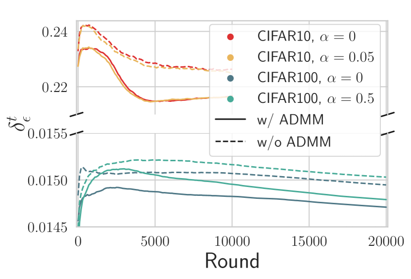
Figure 4: Trend of the difference $\delta_{\operatorname{\boldsymbol{\epsilon}}}^{t}$ (Eq. 6), which decreases as ADMM is used and over training rounds. Cifar datasets, CNN.

with $\beta>0$ being an hyperparameter. Eq. 7 is split into $C$ sub-problems of the form $\operatorname{\boldsymbol{w}}_{k,E}=\operatorname*{arg\,min}_{\operatorname{\boldsymbol{w}}_{k}}\{f_{k}-\sigma_{k}^{\top}(\operatorname{\boldsymbol{w}}^{t}-\operatorname{\boldsymbol{w}}_{k})+\frac{1}{2\beta}\|\operatorname{\boldsymbol{w}}^{t}-\operatorname{\boldsymbol{w}}_{k}^{t}\|^{2}\}$. The local dual variable is updated as $\sigma_{k}\leftarrow\sigma_{k}-\frac{1}{\beta}(\operatorname{\boldsymbol{w}}_{k,E}^{t}-\operatorname{\boldsymbol{w}}_{k,0}^{t})$. The global one $\sigma$ is updated by adding the averaged $\operatorname{\boldsymbol{w}}_{k}-\operatorname{\boldsymbol{w}}^{t}\,\forall k\in\operatorname{\mathcal{C}}$.

Figure 4 confirms the effect of ADMM on gradient alignment: the difference between the true and approximated perturbation, $\delta_{\epsilon}^{t}$ (Eq. 6), decreases over training rounds and with the use of Lagrangian multipliers.

6 Experiments

6.1 Experimental setting

Appendix C details implementation and hyperparameter settings.

Federated datasets. We leverage established FL benchmarks (Caldas et al., 2019; Hsu et al., 2020; 2019). Small-scale image classification: following (Hsu et al., 2020; Caldarola et al., 2022), the federated versions of Cifar10 (10 classes) and Cifar100 (100 classes) (Krizhevsky, 2009) split the respective $50k$ training images in 100 clients with 500 images each. The data distribution is controlled by the Dirichlet’s parameter $\alpha\in\{0,0.05\}$ for Cifar10 and $\{0,0.5\}$ for Cifar100 (Hsu et al., 2019). Lower $\alpha$ signifies increased heterogeneity, with $\alpha=0$ being the most challenging scenario where each client holds samples from one class. Large-scale image classification: Landmarks-User-160k ($2,028$ classes) (Hsu et al., 2020) is the federated Google Landmarks v2 (Weyand et al., 2020) with $164,172$ pictures of worldwide locations, split among $1,262$ realistic clients.

Models. The effectiveness of FedGloSS is shown using multiple model architectures. As in (Hsu et al., 2020; Caldarola et al., 2022), we use a Convolutional Neural Network (CNN) similar to LeNet5 (LeCun et al., 1998) on both Cifar10 ($T=10k$) and Cifar100 ($T=20k$). Experiments with ResNet18 (He et al., 2015) run for $10k$ rounds. For Landmarks-User-160k, we train MobileNetv2 (Sandler et al., 2018; Hsu et al., 2020) ($T=1.3k$), considering the limited resources at the edge.

Baselines. To study real-world settings with varying participation, a small fraction of clients is sampled at each round, with participation rate set to $5\%$ with the CNN and $10\%$ with ResNet18 on both Cifars, and to 50 clients per round in Landmarks-User-160k ($\approx 4\%$). FedGloSS is compatible with any local optimizer (Section 5). We choose SGD and SAM to comply with previous works and compare it with state-of-the-art (SOTA) methods for statistical heterogeneity in FL, distinguishing the results by optimizer type to highlight performance differences. Sgd-based approaches are FedAvg (McMahan et al., 2017), FedProx (Li et al., 2020c), FedDyn (Acar et al., 2021) and Scaffold (Karimireddy et al., 2020b), while use Sam FedSAM (Caldarola et al., 2022; Qu et al., 2022), FedDyn + SAM, FedSpeed (Sun et al., 2023b), FedGamma (Dai et al., 2023) and FedSmoo (Sun et al., 2023a).

6.2 Achieving Local-Global Sharpness Consistency

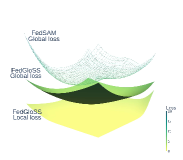
(a) Local model on class sea
w/ FedGloSS

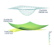
(b) Local model on class snail w/ FedGloSS

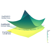
(c) Local model on class sea
w/ FedSmoo

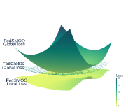
(d) Local model on class snail w/ FedSmoo

Figure 5: Global vs. local perspective of FedGloSS and FedSmoo. Loss landscapes of clients models trained on one class, tested on the local (“Local loss”) or global dataset (“Global loss”). Cifar100 $\alpha=0$ with Sam as local optimizer @ $t=20k$, CNN. (a)-(b): Models trained with FedGloSS. Global loss of FedSam’s local model (net) as reference. (c)-(d): Models trained with FedSmoo. Global loss of FedGloSS’ local model (net) as reference. FedGloSS achieves better consistency w.r.t. FedSmoo.

To assess the effectiveness of FedGloSS in promoting consistency between local and global loss landscapes, Fig. 5 replicates the analysis previously conducted on FedSam (Fig. 2) for direct comparison. The behavior of local models is shown from both local and global perspectives (“Local loss” and “Global loss”, respectively). Section B.1 offers visualizations for the remaining clients. Compared to FedSam, the gap between local and global loss landscapes in FedGloSS is significantly smaller, and both global and local loss surfaces are found in flat and low-loss regions (Figs. 5(a) and 5(b)). This suggests our method effectively promotes convergence toward aligned low-loss flat regions, minimizing the discrepancy between local and global geometries. This results in a global model residing in a flat minimum in the global landscape (Figs. 6(a) and 6(c)). Figs. 5(c) and 5(d) instead compare FedGloSS with the best-performing SOTA FedSmoo, where the position in the global landscape of FedGloSS’ local models is added for reference. While FedSmoo improves consistency between local and global sharpness compared to FedSam, it falls short of FedGloSS in reaching a flatter global minimum.

Table 1 confirms these claims. By combining ADMM for consistency and server-side Sam for global flatness, FedGloSS prioritizes achieving a flatter global region during training, as proven by the lowest global maximum eigenvalue $\lambda_{1,g}$ and larger $\lambda_{1,l}$, across all clients and methods.

6.3 Benchmarking FedGloSS against SOTA

(a) C10 $\alpha=0$ CNN
FedGloSS vs. FedSam

(b) C10 $\alpha=0$ CNN
FedGloSS vs. FedSmoo

(c) C100 $\alpha=0$ CNN
FedGloSS vs. FedSam

(d) C100 $\alpha=0$ CNN
FedGloSS vs. FedSmoo

(e) C10 $\alpha=0.05$ ResNet18
FedGloSS vs. FedSam

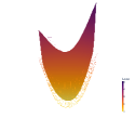
(f) C10 $\alpha=0.05$ ResNet18
FedGloSS vs. FedSmoo

Figure 6: Loss landscapes of models trained with FedGloSS (net) vs. FedSam and FedSmoo (solid) on Cifar10/100. (a) - (c) - (e): The flatter regions reached by FedGloSS w.r.t. FedSam prove the effectiveness of optimizing for global flatness. (b) - (d) - (f): FedGloSS achieves flatter minima and lower loss values w.r.t. FedSmoo.

Table 3: FedGloSS vs. the state of the art on Cifar datasets, distinguished by local optimizer, Sgd (top) and Sam (bottom), in terms of communication cost and accuracy (%). Best results in bold.

			CNN								ResNet18
	Method	Comm.	Cifar10				Cifar100				Cifar10		Cifar100
		Cost	$\alpha=0$		$\alpha=0.05$		$\alpha=0$		$\alpha=0.5$		$\alpha=0.05$		$\alpha=0.5$
Client Sgd	FedAvg	$1\times$	$59.9\scriptscriptstyle{\pm 0.4}$		$65.7\scriptscriptstyle{\pm 1.0}$		$28.6\scriptscriptstyle{\pm 0.7}$		$38.5\scriptscriptstyle{\pm 0.5}$		$72.6\scriptscriptstyle{\pm 0.1}$		$37.4\scriptscriptstyle{\pm 0.2}$
	FedProx	$1\times$	$59.8\scriptscriptstyle{\pm 0.5}$		$65.6\scriptscriptstyle{\pm 1.0}$		$28.8\scriptscriptstyle{\pm 0.7}$		$38.7\scriptscriptstyle{\pm}0.4$		$72.2\scriptscriptstyle{\pm 0.2}$		$37.6\scriptscriptstyle{\pm 0.1}$
	FedDyn	$1\times$	$65.5\scriptscriptstyle{\pm 0.3}$		$70.1\scriptscriptstyle{\pm 1.2}$		✗		✗		$70.2\scriptscriptstyle{\pm 0.6}$		$38.8\scriptscriptstyle{\pm 0.6}$
	Scaffold	$2\times$	$25.1\scriptscriptstyle{\pm 3.7}$		$54.0\scriptscriptstyle{\pm 2.6}$		✗		$30.0\scriptscriptstyle{\pm 1.1}$		$70.8\scriptscriptstyle{\pm 0.6}$		$38.6\scriptscriptstyle{\pm 0.1}$
2-14[1pt/3pt]	FedGloSS	$1\times$	$69.5\scriptscriptstyle{\pm 0.4}$		$75.5\scriptscriptstyle{\pm 0.3}$		$42.5\scriptscriptstyle{\pm 0.6}$		$47.9\scriptscriptstyle{\pm 0.5}$		$79.1\scriptscriptstyle{\pm 0.5}$		$46.7\scriptscriptstyle{\pm 0.6}$
Client Sam	FedSam	$1\times$	$70.2\scriptscriptstyle{\pm 0.9}$		$71.5\scriptscriptstyle{\pm 1.08}$		$28.7\scriptscriptstyle{\pm 0.5}$		$39.6\scriptscriptstyle{\pm 0.5}$		$72.8\scriptscriptstyle{\pm 0.1}$		$38.5\scriptscriptstyle{\pm 0.1}$
	FedDyn	$1\times$	$79.3\scriptscriptstyle{\pm 3.1}$		$81.5\scriptscriptstyle{\pm 0.6}$		✗		✗		$72.6\scriptscriptstyle{\pm 0.2}$		$39.6\scriptscriptstyle{\pm 0.8}$
	FedSpeed	$1\times$	$70.9\scriptscriptstyle{\pm 0.4}$		$72.3\scriptscriptstyle{\pm 1.1}$		$28.9\scriptscriptstyle{\pm 0.5}$		$39.7\scriptscriptstyle{\pm 0.5}$		$72.6\scriptscriptstyle{\pm 0.1}$		$38.8\scriptscriptstyle{\pm 0.6}$
	FedGamma	$2\times$	$58.9\scriptscriptstyle{\pm 1.8}$		$61.9\scriptscriptstyle{\pm 1.8}$		✗		$29.4\scriptscriptstyle{\pm 1.4}$		$72.2\scriptscriptstyle{\pm 0.1}$		$38.8\scriptscriptstyle{\pm 0.3}$
	FedSmoo	$2\times$	$81.3\scriptscriptstyle{\pm 0.5}$		$82.8\scriptscriptstyle{\pm 0.6}$		$47.8\scriptscriptstyle{\pm 0.5}$		$51.7\scriptscriptstyle{\pm 0.46}$		$75.3\scriptscriptstyle{\pm 0.6}$		$44.8\scriptscriptstyle{\pm 0.5}$
2-14[1pt/3pt]	FedGloSS	$1\times$	$83.9\scriptscriptstyle{\pm 0.4}$		$84.4\scriptscriptstyle{\pm 0.5}$		$50.6\scriptscriptstyle{\pm 0.6}$		$53.4\scriptscriptstyle{\pm 0.5}$		$80.0\scriptscriptstyle{\pm 0.3}$		$47.2\scriptscriptstyle{\pm 0.2}$

This section compares FedGloSS with SOTA methods (Section 6.1) on vision tasks in heterogeneous federated settings. Section B.4 discusses results in homogeneous FL.

6.3.1 FedGloSS on Standard Federated Benchmarks

Table 3 presents results on Cifar100 and Cifar10 with varying levels of heterogeneity on the CNN model. Several observations highlight the advantages of FedGloSS. It is straightforward to notice how FedGloSS achieves the best results among both Sgd and Sam-based approaches while maintaining communication efficiency. FedGloSS with local Sam consistently outperforms the best-performing SOTA FedSmoo by $\approx 2.5$ percentage points in accuracy across all dataset configurations with half the communication cost. FedGloSS also reaches the flattest global minima (e.g., $\lambda_{1}^{\textsc{FedGloSS}}=2.03$ vs. $\lambda_{1}^{\textsc{FedSmoo}}=15.37$ on Cifar10 with $\alpha=0$), as shown in Figs. 7 and 6, achieving the best overall performance. FedGloSS with local Sgd overcomes by $\approx 4$ percentage points all Sgd-based approaches. As studied in (Varno et al., 2022), FedDyn suffers from parameter explosion in highly heterogeneous settings, failing to converge on Cifar100. Differently, FedGloSS successfully employs ADMM to align global and local solutions, with the best results under extreme heterogeneity. Similarly, studies showed Scaffold performs poorly in complex heterogeneous environments (Li et al., 2022; Caldarola et al., 2022), resulting in its inability to converge on Cifar100 alongside FedGamma. Lastly, the last two columns of Table 3 further confirm FedGloSS’ effectiveness, consistently outperforming SOTA methods with the more complex ResNet18 architecture, with $\approx 8$ points higher accuracy w.r.t. FedAvg with both Sgd and Sam, and $+5$ w.r.t. FedSmoo, with the flattest solutions (Figs. 6(e) and 6(f)).

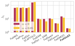
(a) Cifar10

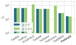
(b) Cifar100

Figure 7: Maximum Hessian eigenvalues ($\lambda_{1}$), CNN. Values shown only if algorithm converged. FedGloSS reaches the flattest global minima.

6.3.2 FedGloSS on Real-World Large-Scale Datasets

To further highlight FedGloSS’s effectiveness, we evaluate it on large-scale image classification using the challenging Landmarks-User-160k dataset. LABEL:tab:sota_gld compares FedGloSS with local Sam against the best-performing baselines. FedGloSS is among the few methods, alongside FedSam and FedSmoo, outperforming FedAvg. Similarly to the Cifar100 results (Section 6.3.1), both Scaffold and FedGamma fail to converge. Importantly, FedGloSS achieves the best overall performance ($+3.4\%$ w.r.t. FedAvg) with reduced communication overhead.

Table 4: MobileNetv2 on Landmarks-User-160k.

Method	Comm. cost	Accuracy
FedAvg	$1\times$	$56.3\scriptscriptstyle{\pm 0.2}$
FedProx	$1\times$	$55.0\scriptscriptstyle{\pm 0.2}$
FedDyn	$1\times$	$55.2\scriptscriptstyle{\pm 0.6}$
Scaffold	$2\times$	✗
FedSam	$1\times$	$56.7\scriptscriptstyle{\pm 0.1}$
FedDyn + Sam	$1\times$	$56.0\scriptscriptstyle{\pm 1.3}$
FedGamma	$2\times$	✗
FedSmoo	$2\times$	$59.5\scriptscriptstyle{\pm 0.1}$
1-3 FedGloSS	$1\times$	$59.7\scriptscriptstyle{\pm 1.2}$

6.3.3 ADMM and SAM Interaction in FedGloSS

ADMM-based methods are often prone to parameter explosion in highly heterogeneous FL settings with many clients Varno et al. (2022). This occurs as multiple gradients accumulate in the global dual variable $\sigma$ (Section 5), causing the parameter norms to grow uncontrollably. However, empirical results indicate that this issue is mitigated with Sam (e.g., see FedDyn vs. FedGloSS in Table 3). We hypothesize this is due to Sam ’s nature: by targeting flat minima, it promotes smaller gradient steps and minimal weight updates, resulting in a more stable algorithm. Fig. 8 confirms our hypothesis by showing Sam’s stability effectively lowers parameter norms and the consequent risk of explosion, particularly when Sam is applied directly to the global model, as in FedGloSS.

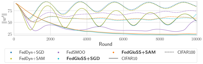
Figure 8: Trend of model parameters norm, $\|\operatorname{\boldsymbol{w}}^{t}\|_{2}$, on Sam-based methods with ResNet18 on Cifar datasets. Sam reduces the norm and the risk of parameters explosion, successfully enabling ADMM in heterogeneous FL.

6.3.4 Communication Efficiency with FedGloSS

Table 5: Communication costs comparison w.r.t. FedAvg. “-” for not reached accuracy, “ ✗” for non-convergence. Gldv2 is Landmarks-User-160k.

Method

CNN

ResNet18

MobileNetv2

Cifar10 $\alpha=0$

Cifar100 $\alpha=0$

Cifar10 $\alpha=0.05$

Cifar100 $\alpha=0.5$

Gldv2

Rounds

Cost

Rounds

Cost

Rounds

Cost

Rounds

Cost

Rounds

Cost

Client Sgd

FedAvg

$10k$

$1B$

$20k$

$1B$

$10k$

$1B$

$10k$

$1B$

$1.3k$

$1B$

FedProx

$7.6k$

$0.8B$

$18.7k$

$0.9B$

$8.8k$

$0.9B$

$8.3k$

$0.8B$

-

-

FedDyn

$2.0k$

$0.2B$

✗

-

-

$3.5k$

$0.4B$

-

-

Scaffold

-

-

-

-

-

-

$8.9k$

$1.8B$

✗

2-17[1pt/3pt]

FedGloSS

$3.4k$

$0.3B$

$5k$

$0.3B$

$2.4k$

$0.2B$

$1.9k$

$0.2B$

$1.3k$

$1B$

Client Sam

FedSam

$6.3k$

$0.6B$

$18.3k$

$0.9B$

$9.2k$

$0.9B$

$7.8k$

$0.8B$

$1.3k$

$1B$

FedDyn

$3.0k$

$0.3B$

✗

$4.1k$

$0.4B$

$3.5k$

$0.4B$

-

-

FedSpeed

$6.3k$

$0.6B$

$18.3k$

0.9B

$8.3k$

$0.8B$

$8.3k$

$0.8B$

$1.3k$

$1B$

FedGamma

-

-

-

-

$9.3k$

$1.9B$

$8.1k$

$1.6B$

✗

FedSmoo

$1.9k$

$0.4B$

$4.5k$

$0.5B$

$2.4k$

$0.5B$

$2.3k$

$0.5B$

$200$

$0.4B$

2-17[1pt/3pt]

FedGloSS

$2.2k$

$0.2B$

$6.3k$

$0.3B$

$2.4k$

$0.2B$

$1.9k$

$0.2B$

$200$

$0.2B$

Communication cost is the main bottleneck in FL (Li et al., 2020a), making its optimization a relevant challenge. As already previously highlighted, FedGloSS considers communication efficiency its primacy concern. Defined $B$ the number of bits exchanged by FedAvg in $T$ training rounds, Table 5 studies FedGloSS’s communication cost against the SOTA baselines in terms of rounds necessary to reach FedAvg’s performance and quantity of exchanged bits. The ADMM-based methods are usually faster, with FedGloSS being the fastest with ResNet18 and MobileNetv2. While FedSmoo is faster when using the CNN model, the transmitted bits double due to its increased communication cost, making FedGloSS the most efficient method in all cases. Analyses on left-out settings in Section B.5.

6.4 Ablation Studies

6.4.1 Communication-efficient Sharpness

This section studies the efficacy of using the pseudo-gradient from the previous round $\tilde{\Delta}_{\operatorname{\boldsymbol{w}}}^{t-1}$ (Eq. 6) as an estimate of the sharpness measure. FedGloSS uses past gradients as a reliable indication on the global loss landscape and, by aligning global and local optimization paths through ADMM, enables consistent trajectories across rounds.

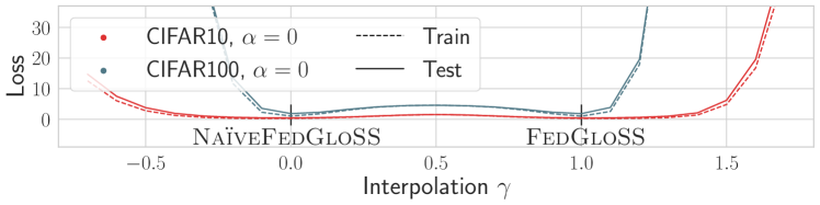
Figure 9: Loss barriers resulting from interpolating NaiveFedGloSS and FedGloSS’ models, which are found in the same basin. Cifar datasets, CNN.

Table 6: FedGloSS vs. NaiveFedGloSS in terms of communication cost, accuracy (50% and 100% of training) and maximum Hessian eigenvalue $\lambda_{1}$. Sam as ClientOpt. Cifar datasets with $\alpha=0$ (top) and $\alpha=0.05/0.5$ (bottom). $\widetilde{\textsc{Sam}}$ is Sam with the sharpness approximation of FedGloSS, using the previous gradient.

Method	Comm.	Cifar10				Cifar100
	Cost	Acc@50%	Acc@100%	$\lambda_{1}$ ($\downarrow$)		Acc@50%	Acc@100%	$\lambda_{1}$ ($\downarrow$)
NaiveFedGloSS	$2\times$	$77.6\scriptscriptstyle{\pm 0.3}$	$83.9\scriptscriptstyle{\pm 0.2}$	$2.78\scriptscriptstyle{\pm 0.13}$		$42.6\scriptscriptstyle{\pm 0.8}$	$50.8\scriptscriptstyle{\pm 0.1}$	$16.93\scriptscriptstyle{\pm 0.27}$
FedGloSS	$1\times$	$78.9\scriptscriptstyle{\pm 0.5}$	$83.9\scriptscriptstyle{\pm 0.4}$	$2.03\scriptscriptstyle{\pm 0.05}$		$39.5\scriptscriptstyle{\pm 0.9}$	$50.6\scriptscriptstyle{\pm 0.6}$	$17.18\scriptscriptstyle{\pm 0.97}$
NaiveFedGloSS	$2\times$	$78.7\scriptscriptstyle{\pm 0.1}$	$84.4\scriptscriptstyle{\pm 0.2}$	$2.75\scriptscriptstyle{\pm 0.09}$		$49.4\scriptscriptstyle{\pm 0.5}$	$53.7\scriptscriptstyle{\pm 0.3}$	$15.84\scriptscriptstyle{\pm 0.52}$
FedGloSS	$1\times$	$79.7\scriptscriptstyle{\pm 0.4}$	$84.4\scriptscriptstyle{\pm 0.5}$	$1.93\scriptscriptstyle{\pm 0.03}$		$47.2\scriptscriptstyle{\pm 1.1}$	$53.4\scriptscriptstyle{\pm 0.5}$	$16.22\scriptscriptstyle{\pm 0.35}$
Centralized		$87.1$ Sam  $86.3\,\widetilde{\textsc{Sam}}$				$58.4$ Sam  $57.6\,\widetilde{\textsc{Sam}}$

Table 6 compares FedGloSS with its baseline, NaiveFedGloSS (Section 5), which computes the true perturbation $\operatorname{\hat{\boldsymbol{\epsilon}}}^{t}$ at the expense of doubled communication costs. FedGloSS achieves accuracy comparable to NaiveFedGloSS while maintaining communication efficiency, with minimal or negligible gap in performance. This aligns with the observed sharpness of the achieved minima ($\lambda_{1}$). To ensure a fair comparison in communication cost, Table 6 also compares FedGloSS’ final accuracy with NaiveFedGloSS’ performance at 50% training progress, showing that FedGloSS achieves higher accuracy with the same number of exchanges, benefiting from the additional global optimization steps deriving from its communication-efficient strategy. This shows our approximation does not slow convergence. In addition, our strategy in centralized settings lowers the performance w.r.t. Sam, thus reducing our centralized upper bound w.r.t. NaiveFedGloSS. At equal performance, FedGloSS narrows the gap to the upper bound: $-2.4\%$ on Cifar10 with $\alpha=0$ and $-1.9\%$ with $\alpha=0.05$ vs. respectively $-3.2\%$ and $-2.7\%$ of NaiveFedGloSS w.r.t. Sam. In Cifar100 instead, $-7\%$ on $\alpha=0$ and $-4.2\%$ on $\alpha=0.5$ of FedGloSS vs. $-8.1\%$ and $-5.2\%$ of its baseline. Lastly, our sharpness approximation does not steer the optimization path: models trained with FedGloSS and NaiveFedGloSS end up in the same basin (no loss barrier), with similar flatness (Fig. 9). Aiming to reduce the communication bottleneck while achieving superior performance, these results confirm our choice of FedGloSS over NaiveFedGloSS.

6.4.2 The Role of Global Consistency and Flatness

Table 7 isolates the impact of global consistency and global sharpness minimization in FedGloSS. We recall FedAvg with client-side Sam is FedSam and using ADMM only for aligning local and global convergence points is FedDyn. Both components significantly impact performance, with their combination leading FedGloSS to the best overall results. FedGloSS is not prone to parameter explosion, achieving the best results even where FedDyn fails to converge (✗). The flatness of FedGloSS’ solutions w.r.t. FedSam in Fig. 6 confirms the efficacy of its strategy.

Table 7: Efficacy of global sharpness minimization in FedGloSS: ADMM for global consistency and server-side Sam for global sharpness minimization lead to the best performance. Cifars, CNN with $\alpha=0$ and ResNet18 with $\alpha\in\{0.05,0.5\}$.

Client	Method	Global	Global	CNN			ResNet18
Opt		Consistency	Flatness	Cifar10	Cifar100		Cifar10	Cifar100
SAM	FedSam	✗	✗	$70.2\scriptscriptstyle{\pm 0.9}$	$28.7\scriptscriptstyle{\pm 0.5}$		$72.8\scriptscriptstyle{\pm 0.1}$	$38.5\scriptscriptstyle{\pm 0.1}$
	FedDyn	✓	✗	$79.3\scriptscriptstyle{\pm 3.1}$	✗		$72.6\scriptscriptstyle{\pm 0.2}$	$39.6\scriptscriptstyle{\pm 0.8}$
	FedGloSS	✓	✓	$83.9\scriptscriptstyle{\pm 0.4}$	$50.6\scriptscriptstyle{\pm 0.6}$		$80.0\scriptscriptstyle{\pm 0.3}$	$47.2\scriptscriptstyle{\pm 0.2}$
SGD	FedAvg	✗	✗	$59.9\scriptscriptstyle{\pm 0.4}$	$28.6\scriptscriptstyle{\pm 0.7}$		$72.6\scriptscriptstyle{\pm 0.1}$	$37.4\scriptscriptstyle{\pm 0.2}$
	FedDyn	✓	✗	$65.5\scriptscriptstyle{\pm 0.3}$	✗		$70.2\scriptscriptstyle{\pm 0.6}$	$38.8\scriptscriptstyle{\pm 0.6}$
	FedGloSS	✓	✓	$69.5\scriptscriptstyle{\pm 0.4}$	$42.5\scriptscriptstyle{\pm 0.6}$		$79.1\scriptscriptstyle{\pm 0.5}$	$46.7\scriptscriptstyle{\pm 0.6}$

7 Discussion

This work tackled the challenge of limited generalization in heterogeneous Federated Learning (FL), prioritizing communication efficiency for real-world use. Building on research linking poor generalization to sharp minima in the loss landscape, we showed data heterogeneity worsens discrepancies between local and global loss surfaces, a problem not resolved by methods focusing only on local sharpness.

To address this issue, we introduced Federated Global Server-side Sharpness (FedGloSS), which finds flat minima in the global loss landscape using server-side Sharpness-Aware Minimization (SAM). FedGloSS achieves communication efficiency by approximating SAM’s sharpness through past global pseudo-gradients, distinguishing it from prior approaches. In addition, by not constraining the clients to use SAM as local optimizer, FedGloSS’ required computational cost can be adapted depending on the local available resources.

Importantly, this work revealed SAM prevents ADMM-related parameter explosion by guiding optimization along flat directions, which reflects in reduced model parameters’ norm, enabling stable updates in heterogeneous FL. A promising future direction could involve exploring alternative approaches to ADMM to align local and global solutions, with the goal of avoiding stateful clients.

Extensive evaluations showed FedGloSS outperforms state-of-the-art methods in accuracy, flatness of the solution and communication efficiency, making it a strong candidate for real-world FL applications.

Appendix

This appendix is organized as follows:

1. Algorithm: details on FedGloSS’ procedure.

2. The benefits of FedGloSS.

3. Implementation details.

4. Flatness analysis.

Appendix A Algorithm

Algorithm 1 summarizes FedGloSS, using as an example Sgd or Sam as local optimizers, differently highlighted. The comment colors replicate those of Fig. 3.

Algorithm 1 FedGloSS with Sam or Sgd as local optimizers

1:Input: Global model $\operatorname{\boldsymbol{w}}$, clients $\operatorname{\mathcal{C}}$, rounds $T$, local iterations $E$, clients’ learning rate $\eta$, clients’ Sam neighborhood size $\rho_{l}$, FedGloSS neighborhood size $\rho$, Lagrangian hyperparameter $\beta$.

2:Initialize: $\operatorname{\boldsymbol{w}}^{0}$, $\sigma^{0}=\sigma_{k}=0$, $\Delta_{\operatorname{\boldsymbol{w}}}^{0}=0.$

3:for each round $t\in[1,T]$ do

4:  $\operatorname{\tilde{\boldsymbol{\epsilon}}}^{t}(\operatorname{\boldsymbol{w}})=\rho\frac{\Delta_{\operatorname{\boldsymbol{w}}}^{t-1}}{\|\Delta_{\operatorname{\boldsymbol{w}}}^{t-1}\|_{2}}$ $\triangleright$ Global perturbation with previous pseudo-grad

5:  $\tilde{\operatorname{\boldsymbol{w}}}^{t}=\operatorname{\boldsymbol{w}}^{t}+\operatorname{\tilde{\boldsymbol{\epsilon}}}^{t}(\operatorname{\boldsymbol{w}})$ $\triangleright$ Server-side approximated FedGloSS ascent step

6:  Randomly select a subset of clients $\operatorname{\mathcal{C}}^{t}\subset\operatorname{\mathcal{C}}$

7:  for each client $k\in\operatorname{\mathcal{C}}^{t}$ in parallel do

8:   $\operatorname{\boldsymbol{w}}_{k,0}=\tilde{\operatorname{\boldsymbol{w}}}^{t}$ $\triangleright$ Initialize local model with perturbed global model $\operatorname{\tilde{\boldsymbol{w}}}^{t}$

9:   Set iteration counter $i=1$

10:   for each epoch $e\in[1,E]$ do

11:     for each batch $\mathcal{B}\in\mathcal{D}_{k}$ do

12:      $\bm{g}_{k,i}=\nabla f_{\mathcal{B}}(\operatorname{\boldsymbol{w}}_{k,i-1})$ $\triangleright$ Local Sgd gradient

13:      $\hat{\bm{\epsilon}}_{k,i}=\rho_{l}\frac{\bm{g}_{k,i}}{\|\bm{g}_{k,i}\|_{2}}$ $\triangleright$ Sam local perturbation

14:      $\bm{g}_{k,i}=\nabla f_{\mathcal{B}}(\operatorname{\boldsymbol{w}}_{k,i-1}+\hat{\bm{\epsilon}}_{k,i})$ $\triangleright$ Local sharpness-aware gradient

15:      $\operatorname{\boldsymbol{w}}_{k,i}\leftarrow\operatorname{\boldsymbol{w}}_{k,i-1}-\eta[\bm{g}_{k,i}-\sigma_{k}+(\operatorname{\boldsymbol{w}}_{k,i-1}-\operatorname{\boldsymbol{w}}_{k,0})/\beta]$ $\triangleright$ Local update with ADMM

16:      $i\leftarrow i+1$

17:     end for

18:   end for

19:   $\sigma_{k}\leftarrow\sigma_{k}-(\operatorname{\boldsymbol{w}}_{k,E}-\tilde{\operatorname{\boldsymbol{w}}}^{t})/\beta$ $\triangleright$ Update local dual variable

20:   Send back to the server the local updated model $\operatorname{\boldsymbol{w}}_{k}^{t}=\operatorname{\boldsymbol{w}}_{k,E}$

21:  end for

22:  $\sigma^{t+1}=\sigma^{t}-\frac{1}{\beta|\mathcal{C}|}\sum_{k\in\mathcal{C}}(\operatorname{\boldsymbol{w}}_{k}^{t}-\operatorname{\boldsymbol{w}}^{t})$ $\triangleright$ Update global dual variable

23:  $\tilde{\Delta}_{\operatorname{\boldsymbol{w}}}^{t}=\sum_{k\in\operatorname{\mathcal{C}}^{t}}\frac{N_{k}}{N}(\tilde{\operatorname{\boldsymbol{w}}}^{t}-\operatorname{\boldsymbol{w}}_{k}^{t})$$\triangleright$ Global pseudo-gradient

24:  $\operatorname{\boldsymbol{w}}^{t+1}=\operatorname{\boldsymbol{w}}^{t}-\tilde{\Delta}_{\operatorname{\boldsymbol{w}}}^{t}-\beta\sigma^{t+1}$ $\triangleright$ FedGloSS descent step w/ pseudo-grad using ADMM

25:end for

Appendix B The Benefits of FedGloSS

B.1 Achieving Consistency on Local and Global Sharpness with FedGloSS

This section completes the analyses presented in Sections 4 and 6.2, showing how FedGloSS guides towards consistent local and global flat loss landscapes. Fig. 10 extends Figs. 5(a) and 5(b) from the main paper with the 3 remaining clients (out of 5) selected in the last round, comparing the behavior of clients’ models trained with FedGloSS from the local and global perspectives. These results highlight the effectiveness of FedGloSS in achieving local models with consistent local-global behavior. Indeed, these models end up in flat regions both in local and global loss landscapes. The comparison with FedSam (net surface) further demonstrates the effectiveness of using our global flatness-aware approach.

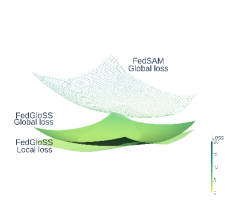
(a) Local model trained
on class bear with FedGloSS

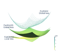
(b) Local model trained on
class skyscraper with FedGloSS

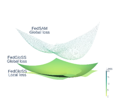
(c) Local model trained
on class possum with FedGloSS

Figure 10: Global vs. local perspective on FedGloSS. Cifar100 $\alpha=0$ with Sam as local optimizer @ $20k$ rounds on CNN. (a) - (c): Local models trained on one class, tested on the local (“Local loss”) or global dataset (“Global loss”). Corresponding global perspective of local model trained with FedSam (net) added as reference.

Fig. 11 instead extends Figs. 5(c) and 5(d), offering a comparative analysis of FedSmoo’s clients’ models w.r.t. FedGloSS (net landscape). The local solutions found by FedGloSS achieve flatter, better (i.e., lower loss) and more consistent convergence points in the global loss landscape w.r.t. our main competitor FedSmoo.

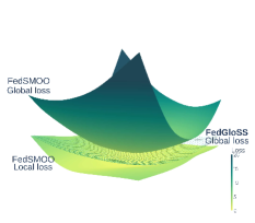
(a) Local model trained
on class bear with FedGloSS

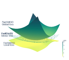
(b) Local model trained on
class skyscraper with FedGloSS

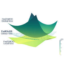
(c) Local model trained
on class possum with FedGloSS

Figure 11: Global vs. local perspective on FedSmoo. Cifar100 $\alpha=0$ with Sam as local optimizer @ $20k$ rounds on CNN. (a) - (c): Local models trained on one class, tested on the local (“Local loss”) or global dataset (“Global loss”). Corresponding global perspective of local model trained with FedGloSS (net) added as reference.

B.2 Achieving Flatter Global Minima

(a) Cifar10 $\alpha=0$

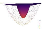
(b) Cifar10 $\alpha=0.05$

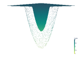
(c) Cifar100 $\alpha=0$

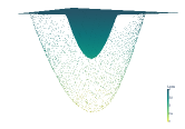
(d) Cifar100 $\alpha=0.5$

Figure 12: Visualization of the loss landscapes of the CNN trained with FedGloSS (net) and the de-facto standard optimization algorithm in FL FedAvg (solid). Comparison with varying degrees of heterogeneity on Cifar10 (left) and Cifar100 (right). FedGloSS consistently achieves flatter minima and lower loss values in the global loss landscape.

FedGloSS vs. FedAvg, FedSam, FedSmoo.

Fig. 12 compares the loss landscapes of global models trained with FedGloSS and FedAvg, showing how the former consistently achieves flatter minima and lower loss values in the global loss landscapes. This confirms the behaviors already appreciated in Fig. 6. In addition, Fig. 13 shows the global loss surfaces of FedGloSS’ solutions against models trained with FedSam and FedSmoo. These plots extend Fig. 6 with the less heterogeneous scenarios $\alpha=0.05$ for Cifar10 and $\alpha=0.5$ on Cifar100. They confirm FedGloSS’ effectiveness in reaching flatter and lower-loss solutions with respect to its main direct competitors.

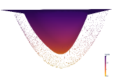
(a) Cifar10 $\alpha=0.05$
FedGloSS vs. FedSam

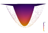
(b) Cifar10 $\alpha=0.05$
FedGloSS vs. FedSmoo

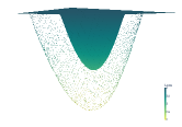
(c) Cifar100 $\alpha=0.5$
FedGloSS vs. FedSam

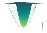
(d) Cifar100 $\alpha=0.5$
FedGloSS vs. FedSmoo

Figure 13: Visualization of the loss landscapes of the CNN trained with FedGloSS (net) and FedSam or FedSmoo (solid). Comparison with $\alpha=0.05$ Cifar10 (left) and $\alpha=0.5$ Cifar100 (right) extending Fig. 6. FedGloSS consistently achieves flatter minima and lower loss values in the global loss landscape.

FedGloSS on ResNet18.

Fig. 14 extends Fig. 6 from the main paper and shows the flatter loss landscapes reached by FedGloSS when using ResNet18 on Cifar10 and Cifar100.

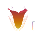
(a) Cifar10 $\alpha=0.05$
FedGloSS (net) vs.
FedAvg (solid)

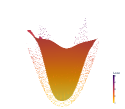
(b) Cifar10 $\alpha=0.05$
FedGloSS (net) vs.
FedSam (solid)

(c) Cifar10 $\alpha=0.05$
FedGloSS (net) vs.
FedSmoo (solid)

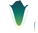
(d) Cifar100 $\alpha=0.5$
FedGloSS (net) vs. FedAvg (solid)

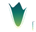
(e) Cifar100 $\alpha=0.5$
FedGloSS (net) vs. FedSam (solid)

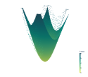
(f) Cifar100 $\alpha=0.5$
FedGloSS (net) vs. FedSmoo (solid)

Figure 14: Visualization of loss landscapes of the ResNet18 trained with FedGloSS (net) and FedAvg, or FedSam or FedSmoo (solid). Comparison with Cifar10 $\alpha=0.05$ (a-c) and Cifar100 $\alpha=0.5$ (d-f). FedGloSS achieves flatter and lower-loss regions in the global landscape.

Hessian Eigenvalues.

Table 8 reports the values of the maximum Hessian eigenvalues, as already shown in Fig. 7 in the main paper. First, as expected, we note that Sam-based methods achieve flatter minima w.r.t. the counterpart. Notably, our main competitor FedSmoo presents higher sharpness than FedSam in the simpler Cifar10, regardless of the data distribution. In addition, FedGloSS with local Sam achieves the lowest sharpness (i.e., lowest $\lambda_{1}$) on all configurations, outperforming the state of the art and, specifically, all sharpness-aware methods.

Table 8: FedGloSS vs. the state of the art, distinguished by local optimizer - Sgd (top) and Sam (bottom). Comparison in terms of communication cost and maximum Hessian eigenvalue $\lambda_{1}$. Best results in bold. Model: CNN.

	Method		Cifar10				Cifar100
		Comm.	$\alpha=0$		$\alpha=0.05$		$\alpha=0$		$\alpha=0.5$
		Cost	$\lambda_{1}(\downarrow)$		$\lambda_{1}(\downarrow)$		$\lambda_{1}(\downarrow)$		$\lambda_{1}(\downarrow)$
Client Sgd	FedAvg	$1\times$	$66.23\pm 0.50$		$71.14\pm 4.07$		$66.30\pm 3.08$		$68.77\pm 0.96$
	FedProx	$1\times$	$66.19\pm 0.52$		$71.41\pm 4.40$		$66.34\pm 3.75$		$68.63\pm 1.37$
	FedDyn	$1\times$	$63.94\pm 4.41$		$71.44\pm 8.73$		-		-
	Scaffold	$2\times$	$166.54\pm 6.93$		$180.51\pm 30.08$		-		$120.01\pm 0.76$
2-14[1pt/3pt]	FedGloSS	$1\times$	$58.26\pm 3.49$		$56.28\pm 4.19$		$96.01\pm 9.00$		$107.35\pm 7.5$
Client Sam	FedSam	$1\times$	$10.35\pm 0.07$		$9.43\pm 0.28$		$58.38\pm 2.93$		$57.54\pm 1.21$
	FedDyn	$1\times$	$10.04\pm 5.38$		$6.58\pm 0.20$		-		-
	FedSpeed	$1\times$	$10.92\pm 0.17$		$9.97\pm 0.12$		$58.23\pm 3.18$		$58.00\pm 1.86$
	FedGamma	$2\times$	$4.79\pm 0.20$		$4.55\pm 0.20$		-		$99.86\pm 6.74$
	FedSmoo	$2\times$	$15.37\pm 1.67$		$12.57\pm 0.56$		$28.43\pm 1.97$		$29.23\pm 0.17$
2-14[1pt/3pt]	FedGloSS	$1\times$	$2.03\pm 0.05$		$1.93\pm 0.03$		$17.18\pm 0.97$		${16.22}\pm 0.35$

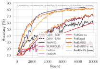
(a) $\alpha=0$ Sam

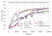
(b) $\alpha=0$ Sgd

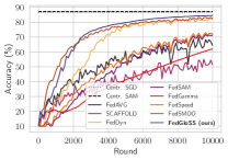
(c) $\alpha=0.05$ Sam

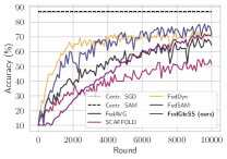
(d) $\alpha=0.05$ Sgd

Figure 15: Cifar10 with varying degrees of heterogeneity ($\alpha\in\{0,0.05\}$). Results of centralized runs (dashed lines) added as reference. Comparison of FedGloSS with state-of-the-art approaches, distinguished in Sam-based methods (a, c) and Sgd-based ones (b, d). FedGloSS consistently achieves the best performance. Model: CNN.

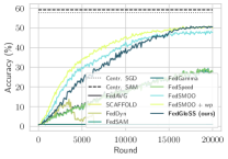
(a) $\alpha=0$ Sam

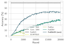
(b) $\alpha=0$ Sgd

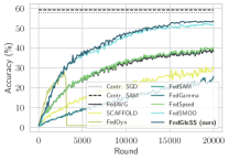
(c) $\alpha=0.5$ Sam

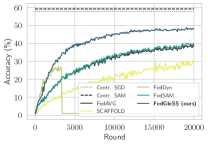
(d) $\alpha=0.5$ Sgd

Figure 16: Cifar100 with varying degrees of heterogeneity ($\alpha\in\{0,0.5\}$) with CNN. Results of centralized runs (dashed lines) added as reference. Comparison of FedGloSS with state-of-the-art approaches, distinguished in Sam-based methods (a, c) and Sgd-based ones (b, d). FedGloSS consistently achieves the best performance.

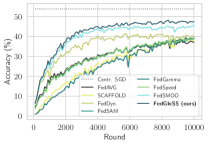
(a) Cifar100 $\alpha=0.5$ Sam

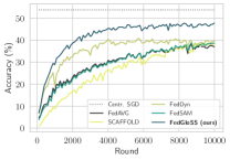
(b) Cifar100 $\alpha=0.5$ Sgd

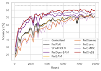
(c) Cifar10 $\alpha=0.05$ Sam

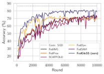
(d) Cifar10 $\alpha=0.05$ Sgd

Figure 17: Accuracy trends with ResNet18 on Cifar100 (left) and Cifar10 (right). Comparison of FedGloSS with state-of-the-art approaches, distinguished in Sam-based methods (a, c) and Sgd-based ones (b, d). FedGloSS consistently achieves the best performance, both in terms of final accuracy and convergence speed.

B.3 Increasing Convergence Speed

Figs. 15 and 16 show the accuracy trends of FedGloSS compared to state-of-the-art methods for heterogeneous FL on Cifar10 and Cifar100 respectively. For a clearer understanding, we distinguish between Sam-based and Sgd-based methods depending on the used local optimizer. For a fair comparison, we report FedSmoo with and without the scheduling of $\rho$ (+wp in the figure). For additional details on the scheduling, refer to Appendix C. FedGloSS consistently achieves the best performances and convergence speedup in each group. In addition, we remind that FedGloSS communicates half the number of bits at each round w.r.t. FedSmoo. Fig. 17 reports the results obtained with ResNet18 on both datasets: FedGloSS consistently achieves the best speed of convergence and final accuracy, with both Sam and Sgd as ClientOpt.

B.4 Effectiveness in Multiple Scenarios and with Several Model Architectures

As already shown in Section 6, FedGloSS outperforms the state of the art in terms of speed of convergence, final performance in accuracy, flatness of the solution and communication efficiency. This remains true across multiple datasets (Cifar100, Cifar10, Landmarks-User-160k) and model architectures (CNN, ResNet18, MobileNetv2). The main paper focuses on results in more challenging heterogeneous FL scenarios. The next paragraph discusses the behavior of FedGloSS in homogeneous settings.

FedGloSS in Homogeneous Settings.

Table 9 evaluates FedGloSS against the main methods FedAvg, FedSam, FedDyn and FedSmoo in homogeneous FL settings. Here, client gradients are naturally more aligned due to reduced client drift (Karimireddy et al., 2020b). We thus test FedGloSS with and without ADMM for global consistency. As expected, FedGloSS achieves similar accuracy with or without ADMM, particularly when using SAM as the local optimizer. However, ADMM facilitates convergence to flatter minima (evidenced by lower $\lambda_{1}$ values) by aligning local and global convergence points. Notably, FedGloSS achieves the flattest minima (lowest $\lambda_{1}$) across both datasets, and the best accuracy on the more complex Cifar100. While FedSmoo achieves slightly higher accuracy on Cifar10, FedGloSS finds a flatter minimum and achieves competitive accuracy with significantly lower communication costs (halved).

Table 9: FedGloSS against SOTA FL methods on homogeneous Cifar settings, compared in terms of communication costs, accuracy (%) and maximum Hessian eigenvalue $\lambda_{1}$. Best result in bold and second best underlined. Model: CNN.

Method	Comm.	ADMM	Cifar10 $\alpha=100$			Cifar100 $\alpha=1000$
	Cost		Accuracy	$\lambda_{1}$		Accuracy	$\lambda_{1}$
FedAvg	$1\times$	✗	84.0	68.4		50.1	49.4
FedSam	$1\times$	✗	84.7	36.2		53.4	32.6
FedDyn (Sgd)	$1\times$	✓	83.8	47.8		51.9	91.7
FedDyn (Sam)	$1\times$	✓	84.5	27.9		52.5	46.0
FedSmoo	$2\times$	✓	85.1	6.4		53.9	24.6
FedGloSS (Sgd)	$1\times$	✗	84.0	67.7		50.5	50.8
	$1\times$	✓	83.1	7.1		51.7	47.9
FedGloSS (Sam)	$1\times$	✗	84.8	36.2		55.8	13.9
	$1\times$	✓	84.8	2.8		55.7	11.8

B.5 Reducing Communication Costs

Analysis on communication cost.

Table 10 extends the analysis presented in Section 6.3.4 by evaluating the communication costs across all scenarios considered in this work. Notably, since FedGloSS maintains the per-round communication cost of FedAvg, it remains advantageous even when matching the convergence speed of the best-performing algorithm (FedSmoo), due to its halved communication costs.

Table 10: Communication costs comparison w.r.t. FedAvg. “-” for not reached accuracy, “✗” for non-convergence.

	Method		CNN												ResNet18						MobileNetv2
			Cifar-10						Cifar-100						Cifar-10			Cifar-100			Landmarks-User-160k
			$\alpha=0$			$\alpha=0.05$			$\alpha=0$			$\alpha=0.5$			$\alpha=0.05$			$\alpha=0.5$
			Rounds	Cost		Rounds	Cost		Rounds	Cost		Rounds	Cost		Rounds	Cost		Rounds	Cost		Rounds	Cost
Sgd-based	FedAvg		$10k\ (1\times)$	$1B$		$10k\ (1\times)$	$1B$		$20k\ (1\times)$	$1B$		$20k\ (1\times)$	$1B$		$10k\ (1\times)$	$1B$		$10k\ (1\times)$	$1B$		$1.3k\ (1\times)$	$1B$
	FedProx		$7.6k\ (1.3\times)$	$0.8B$		$7.9k\ (1.3\times)$	$0.8B$		$18.7k\ (1.1\times)$	$0.9B$		$18.6k\ (1.1\times)$	$0.9B$		$8.8k\ (1.1\times)$	$0.9B$		$8.3k(1.2\times)$	$0.8B$		-	-
	FedDyn		$2k\ (5\times)$	$0.2B$		$1.9k\ (5\times)$	$0.2B$		✗			✗			-	-		$3.5k\ (2.9\times)$	$0.4B$		-	-
	Scaffold		-	-		-	-		-	-		-	-		-	-		$8.9k\ (1.1\times)$	$1.8B$		✗
2-23[1pt/3pt]	FedGloSS		$3.4k\ (2.9\times)$	$0.3B$		$3.8k\ (2.6\times)$	$0.4B$		$5k\ (4\times)$	$0.3B$		$4.7k\ (4.3\times)$	$0.2B$		$2.4k\ (4.2\times)$	$0.2B$		$1.9k\ (5.3\times)$	$0.2B$		-	-
Sam-based	FedSam		$6.3k\ (1.6\times)$	$0.6B$		$7.8k\ (1.3\times)$	$0.8B$		$18.3k\ (1.1\times)$	$0.9B$		$16.3k\ (1.2\times)$	$0.8B$		$9.2k\ (1.1\times)$	$0.9B$		$7.8k\ (1.3\times)$	$0.8B$		$1.3k\ (1\times)$	$1B$
	FedDyn		$3k\ (3.3\times)$	$0.3B$		$4.2k\ (2.4\times)$	$0.4B$		✗			✗			$4.1k\ (2.4\times)$	$0.4B$		$3.5k\ (2.9\times)$	$0.4B$		-	-
	FedSpeed		$6.3k\ (1.6\times)$	$0.6B$		$6.9k\ (1.4\times)$	$0.7B$		$18.3k\ (1.1\times)$	$0.9B$		$15.7k\ (1.3\times)$	0.8B		$8.3k\ (1.2\times)$	$0.8B$		$8.3k\ (1.2\times)$	$0.8B$		$1.3k\ (1\times)$	$1B$
	FedGamma		-	-		-	-		-	-		-	-		$9.3k\ (1.1\times)$	$1.9B$		$8.1k\ (1.2\times)$	$1.6B$		✗
	FedSmoo		$1.9k\ (5.3\times)$	$0.4B$		$2.2k\ (4.5\times)$	$0.4B$		$4.5k\ (4.4\times)$	$0.5B$		$6.5k\ (3.1\times)$	$0.7B$		$2.4k\ (4.2\times)$	$0.5B$		$2.3k\ (4.3\times)$	$0.5B$		$200\ (6.5\times)$	$0.3B$
2-23[1pt/3pt]	FedGloSS		$2.2k\ (4.5\times)$	$0.2B$		$2.2k\ (4.5\times)$	$0.2B$		$6.3k\ (3.2\times)$	$0.3B$		$5.2k\ (3.8\times)$	$0.3B$		$2.4k\ (4.2\times)$	$0.2B$		$1.9k\ (5.3\times)$	$0.2B$		$200\ (6.5\times)$	$0.2B$

FedGloSS vs. NaiveFedGloSS.

Fig. 18 deepens the comparison between FedGloSS and its baseline NaiveFedGloSS, discussed in Section 6.4. In particular, this plot reports the accuracy trends of the two methods, showing that NaiveFedGloSS is slightly faster ($\approx 1.1\times$) than FedGloSS in Cifar100, while FedGloSS surpasses the speed of the baseline after $\approx 25\%$ of training in Cifar10. However, both methods reach the same accuracy at the of training. In addition, it is to be noted that FedGloSS halves the communication cost w.r.t. NaiveFedGloSS by transmitting half the number of bits at each round. Additionally, it also reduces the communication cost by half, as it eliminates the need to invoke the clients twice to compute the updates. These insights further support our choice of the efficient strategy of FedGloSS over NaiveFedGloSS.

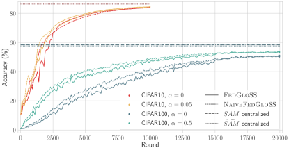
Figure 18: Accuracy trends of FedGloSS vs. NaiveFedGloSS. The comparison includes the centralized upper bounds of Sam and $\widetilde{\text{{Sam}}}$ (the adaptation of FedGloSS’ strategy to the centralized scenario). CNN on Cifar10 and Cifar100 with varying heterogeneity degree ($\alpha$). NaiveFedGloSS is $\approx 1.1\times$ faster than its efficient alternative FedGloSS in Cifar100, while FedGloSS shows increased convergence speed after $\approx 25\%$ of training rounds in Cifar10. However, both methods reach the same accuracy at the of training. These results motivate the choice of FedGloSS over NaiveFedGloSS.

Convergence speed.

Since all methods are compared over a fixed amount of communication rounds, higher final accuracy implies faster convergence. Since FedGloSS consistently outperforms the other state-of-the-art algorithms taken into account, it is guaranteed to converge faster, as also shown in the accuracy trends (Figs. 15, 16 and 17).

B.6 The Impact of Server-side $\rho_{s}$

Fig. 19 analyzes the impact of $\rho_{s}$ on the performance of the global model, both in terms of accuracy (Fig. 19(a)) and flatness of the solution (Fig. 19(b)). In details, Fig. 19(a) compares the accuracy of the global model trained on Cifar100 when varying the model architecture (CNN vs. ResNet18) and the data heterogeneity ($\alpha=0$ vs. $\alpha=0.5$). In all the configurations, we note that a smaller value of $\rho_{s}$ usually leads to the best results. Fig. 19(b) instead focuses on the CNN in the most heterogeneous setting ($\alpha=0$) and compares the reached accuracy with the corresponding maximum Hessian eigenvalue $\lambda_{1}$ when varying $\rho_{s}$. A larger server-side $\rho_{s}$ corresponds to a smaller $\lambda_{1}$, i.e., a flatter region in the global loss landscape.

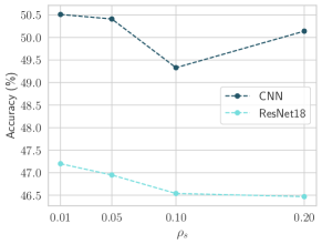
(a) FedGloSS $\rho_{s}$ with different architectures

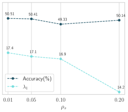
(b) FedGloSS $\rho_{s}$ vs. $\lambda_{1}$

Figure 19: Cifar100. (a): Accuracy (%) of FedGloSS when varying the server-side Sam $\rho_{s}$, with different heterogeneity and architecture (CNN with $\alpha=0$ and ResNet18 with $\alpha=0.5$). Smaller values of $\rho_{s}$ lead to better performances. (b): FedGloSS $\rho_{s}$ vs. maximum Hessian eigenvalue $\lambda_{1}$ on CNN with $\alpha=0$. Larger values of $\rho_{s}$ lead to lower eigenvalues with minimum loss in accuracy.

Appendix C Implementation Details

This section delves into a comprehensive description of the datasets and models utilized throughout this paper, specifying the Deep Learning framework and the hardware employed (Section C.1). Additionally, we present the area of the hyper-parameters’ space explored during the fine-tuning process in order to yield optimal results (Section C.2).

C.1 Datasets and Models

Table 11 provides a comprehensive overview of each dataset’s general statistics. This includes the number of training clients participating in the process and the total number of samples used to construct both the training and test sets.

Table 11: Datasets’ description with their general statistics on the size and number of clients.

Dataset	Train clients		Train samples		Test samples
Cifar10	100		50,000		10,000
Cifar100	100		50,000		10,000
Landmarks-User-160k	1262		164,172		19,526

C.1.1 Cifar10 and Cifar100

We adapted these two well-known image classification datasets to the FL scenario by replicating the splits among clients proposed by (Hsu et al., 2019). Both datasets are split evenly among 100 clients, thus each of them has access to 500 data samples. This partitioning is performed according to a Latent Dirichlet Allocation (LDA) on the labels. In practice, each local dataset follows a multinomial distribution drawn according to a symmetric Dirichlet distribution with concentration parameter $\alpha$. The higher the value of this parameter is, the more the local datasets resemble a homogeneous scenario, in the limit case $\alpha=0$ each client has access to one only class of images. In our experiments we tested $\alpha\in\{0,0.05,100\}$ and $\alpha\in\{0,0.5,1000\}$ for Cifar10 and Cifar100, respectively. Figs. 20(a) and 20(b) show how data is distributed across clients in all the experimental settings for these two datasets. Both datasets are pre-processed by applying random crops and random horizontal flips.

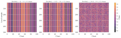
(a) Cifar10

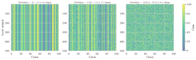
(b) Cifar100

Figure 20: Cifar10 (left) and Cifar100 (right) data distribution across clients with the heterogeneity levels tested in the experiments. On top of each chart we report the average number of classes seen by each client.

Models.

We trained a Convolutional Neural Network (CNN) inspired by the LeNet-5 architecture (LeCun et al., 1998), as proposed by (Hsu et al., 2020). The network comprises two 64-channels convolutional layers, both using $5\times 5$ kernels and followed by $2\times 2$ max-pooling layers. This is succeeded by two fully-connected layers with 384 and 192 units, respectively. The final output layer is adapted to the specific number of classes in the dataset.

To explore deeper and more expressive architectures, we also trained a ResNet18 (He et al., 2015) on Cifar100 with $\alpha=0.5$ and Cifar10 with $\alpha=0.05$. We replaced the standard Batch Normalization layers (Ioffe & Szegedy, 2015) with Group Normalization layers (Wu & He, 2018) due to their demonstrated effectiveness in handling skewed data distributions in FL (Hsieh et al., 2020). We carried out the experiments with the CNN model using PyTorch (Paszke et al., 2019) and the ResNet18 ones using FedJAX (Ro et al., 2021).

C.1.2 Landmarks-User-160k

To achieve a comprehensive understanding of the efficacy of the proposed method, a thorough analysis was undertaken utilizing large-scale real-world datasets. Specifically, we use the Landmarks-User-160k dataset (Hsu et al., 2020), a repository encompassing 164,172 images depicting 2028 distinct landmarks, distributed among 1262 clients.

Models.

The model employed for training is a MobileNetV2 (Sandler et al., 2018; Hsu et al., 2020), replacing batch normalization with group normalization layers and pre-trained on ImageNet (Deng et al., 2009). The tests on this dataset were carried out on a cluster of NVIDIA A100 40GB, using our FedJAX codebase.

C.2 Hyperparameters

In Table 12 we report the training hyperparameters associated to each dataset and model pairing. While Table 13 summarizes the hyper-parameters search grid tested for each method (in bold the chosen ones). All runs are averaged over 3 seeds. In addition, following previous works (Acar et al., 2021; Caldarola et al., 2022; 2023), we report the averaged accuracy of the last 100 rounds to reduce the noise typical of heterogeneous FL settings.

While running our experiments on FedGloSS, we noticed that a larger value of local $\rho$ allowed to reach the best final accuracy, while a smaller $\rho$ achieved faster convergence in the initial training stages. Following this insight, we schedule the value of $\rho$ for $T_{s}$ rounds as

$$\rho(t)=\begin{cases}\rho_{0}+\nicefrac{{(\rho-\rho_{0})}}{{T_{s}}}\cdot t&\text{if $t\leq T_{s}$}\\ \rho&\text{otherwise,}\\ \end{cases}$$

starting from the value $\rho_{0}=0.001$.

Table 12: General training hyper-parameters common to all methods, distinguished by dataset and model architecture. Symbols: local epochs $E$, local learning rate $\eta$, weight decay $wd$, client-side momentum $\beta_{l}$, batch size $B$.

Dataset	Model	Rounds	Clients		Client optimization
			per round		$E$	$\eta$	$wd$	$\beta_{l}$	$B$
Cifar10	CNN	10000	5		1	$10^{-2}$	$4\cdot 10^{-4}$	0	64
1-10[1pt/3pt] Cifar100	CNN	20000	5		1	$10^{-2}$	$4\cdot 10^{-4}$	0	64
	ResNet18-GN	10000	10		1	$10^{-2}$	$10^{-5}$	0.7	64
1-10[1pt/3pt] Landmarks-User-160k	MobileNetv2	1300	50		5	0.1	$4\cdot 10^{-5}$	0	64

Table 13: Search grid used to find optimal hyper-parameters for each combination of method, dataset and model. We highlight the best performing values in bold.

Method	HParam		Cifar10			Cifar100			Landmarks-User-160k
			CNN	ResNet18		CNN	ResNet18
FedSam	$\rho$		[0.05, 0.1, 0.15, 0.2]	[0.01, 0.02, 0.05]		[0.005, 0.01, 0.02, 0.05]	[0.01, 0.02, 0.05]		[0.05]
FedProx	$\mu$		[0.001, 0.01, 0.1]	[0.001, 0.01, 0.1]		[0.001, 0.01, 0.1]	[0.001, 0.01, 0.1]		[0.001, 0.01, 0.1]
FedDyn	$\alpha$		[0.001, 0.01, 0.1]	[0.001, 0.01, 0.1]		[0.001, 0.01, 0.1]	[0.01]		[0.001, 0.01]
	$\rho$ (Sam-based only)		[0.15]	[0.01]		[0.01, 0.02]	[0.01]		[0.05]
FedSpeed	$\rho$		[0.05, 0.1, 0.15, 0.2]	[0.01]		[0.005, 0.01, 0.02, 0.05]	[0.01]		[0.05]
	$\alpha$		[0.9, 0.95, 0.99]	[0.9, 0.95]		[0.9, 0.95, 0.99]	[0.9, 0.95]		[0.95]
	$\lambda$		[10, 100, 1000]	[10, 100, 1000]		[10, 100, 1000]	[10, 100, 1000]		[100, 1000]
FedGamma	$\rho$		[0.15]	[0.01]		[0.01]	[0.01]		[0.05]
FedSmoo	$\rho$		[0.05, 0.1, 0.15, 0.2]	[0.01]		[0.005, 0.01, 0.05, 0.1, 0.2]	[0.01]		[0.05, 0.1, 0.2, 0.3]
	$\beta$		[5, 10, 100]	[1, 2, 5, 10]		[10, 100]	[5, 10, 100]		[10, 50, 100, 1000]
FedGloSS (ours)	$\rho_{s}$		[0.01, 0.1, 0.15]	[0.01, 0.05, 0.1, 0.5]		[0.01, 0.05, 0.1, 0.2]	[0.01, 0.05, 0.1, 0.5]		[0.005, 0.01, 0.02]
	$\rho$		[0.05, 0.1, 0.15, 0.2]	[0.01]		[0.05, 0.1, 0.2]	[0.01]		[0.05, 0.1, 0.2, 0.3]
	$\beta$		[5, 10, 100]	[1, 2, 5, 10]		[10, 100]	[5, 10, 100]		[10, 50, 100]
	$T_{s}$		[1000, 2000, 4000]	[0]		[1000, 2000, 5000, 10000, 15000]	[0]		[0]

Appendix D Flatness Analysis

This section describes the procedure to compute the visualization of the loss landscapes and the Hessian eigenvalues.

D.1 Visualizing 1D Loss Landscapes

Fig. 9 in the main paper shows the interpolation of FedGloSS and NaiveFedGloSS’s models. Given their respective weights $\operatorname{\boldsymbol{w}}_{\textsc{FedGloSS}}$ and $\operatorname{\boldsymbol{w}}_{\textsc{NaiveFedGloSS}}$, the interpolation is computed using a coefficient $\gamma$ as

$$\operatorname{\boldsymbol{w}}=\gamma\cdot\operatorname{\boldsymbol{w}}_{\textsc{FedGloSS}}+(1-\gamma)\cdot\operatorname{\boldsymbol{w}}_{\textsc{NaiveFedGloSS}}.$$ (8)

For each $\gamma\in[-1,2]$, $\operatorname{\boldsymbol{w}}$ is tested on the training or test sets, and the plot reports the computed loss. The resulting interpolation indicates that there is no loss barrier between the two models, suggesting they lie within the same basin. Additionally, the 1D geometry of the emerging loss landscape reveals that both models converge to a flat minimum when evaluated on both Cifar100 and Cifar10.

D.2 Visualizing 3D Loss Landscapes

We leverage techniques from (Li et al., 2018) to visualize the loss landscapes of our models. We adapt their code to work with our specific datasets and network architectures. The process involves calculating the loss function along random directions in the parameter space. This is achieved by perturbing the model’s parameters within a defined range. In our visualizations, we constrain these perturbations to occur within the range of $[-1,1]$ for both the $x$ and $y$ axes. To ensure consistent comparisons across models (e.g., as seen in Fig. 6), we utilize the same set of random directions for all models.

D.3 Hessian Eigenvalues for Flatness Measure

Following prior work (Foret et al., 2021; Garipov et al., 2018; Li et al., 2018; Caldarola et al., 2022), we use the spectrum of the Hessian matrix to quantify the flatness of the loss landscape. Here, lower maximum eigenvalues correspond to flatter landscapes, implying less sharpness. To compute these eigenvalues (denoted by $\lambda_{1}$ in the main paper), we employ the stochastic power iteration method (Xu et al., 2018) with a maximum of 20 iterations, referring to the code of Golmant et al. (2018).

References

- Acar et al. (2021) Durmus Alp Emre Acar, Yue Zhao, Ramon Matas Navarro, Matthew Mattina, Paul N Whatmough, and Venkatesh Saligrama. Federated learning based on dynamic regularization. ICLR, 2021.
- Antunes et al. (2022) Rodolfo Stoffel Antunes, Cristiano André da Costa, Arne Küderle, Imrana Abdullahi Yari, and Björn Eskofier. Federated learning for healthcare: Systematic review and architecture proposal. ACM Transactions on Intelligent Systems and Technology (TIST), 13(4):1–23, 2022.
- Boyd et al. (2011) Stephen Boyd, Neal Parikh, Eric Chu, Borja Peleato, Jonathan Eckstein, et al. Distributed optimization and statistical learning via the alternating direction method of multipliers. Foundations and Trends® in Machine learning, 3(1):1–122, 2011.
- Caldarola et al. (2022) Debora Caldarola, Barbara Caputo, and Marco Ciccone. Improving generalization in federated learning by seeking flat minima. In European Conference on Computer Vision, pp. 654–672. Springer, 2022.
- Caldarola et al. (2023) Debora Caldarola, Barbara Caputo, and Marco Ciccone. Window-based model averaging improves generalization in heterogeneous federated learning. In Proceedings of the IEEE/CVF International Conference on Computer Vision, pp. 2263–2271, 2023.
- Caldas et al. (2019) Sebastian Caldas, Sai Meher Karthik Duddu, Peter Wu, Tian Li, Jakub Konečnỳ, H Brendan McMahan, Virginia Smith, and Ameet Talwalkar. Leaf: A benchmark for federated settings. Workshop on Data Privacy and Confidentiality, 2019.
- Dai et al. (2023) Rong Dai, Xun Yang, Yan Sun, Li Shen, Xinmei Tian, Meng Wang, and Yongdong Zhang. Fedgamma: Federated learning with global sharpness-aware minimization. IEEE Transactions on Neural Networks and Learning Systems, 2023.
- Deng et al. (2009) Jia Deng, Wei Dong, Richard Socher, Li-Jia Li, Kai Li, and Li Fei-Fei. Imagenet: A large-scale hierarchical image database. In 2009 IEEE conference on computer vision and pattern recognition, pp. 248–255. Ieee, 2009.
- Du et al. (2022a) Jiawei Du, Hanshu Yan, Jiashi Feng, Joey Tianyi Zhou, Liangli Zhen, Rick Siow Mong Goh, and Vincent YF Tan. Efficient sharpness-aware minimization for improved training of neural networks. ICLR, 2022a.
- Du et al. (2022b) Jiawei Du, Daquan Zhou, Jiashi Feng, Vincent Tan, and Joey Tianyi Zhou. Sharpness-aware training for free. Advances in Neural Information Processing Systems, 35:23439–23451, 2022b.
- Fantauzzo et al. (2022) Lidia Fantauzzo, Eros Fanì, Debora Caldarola, Antonio Tavera, Fabio Cermelli, Marco Ciccone, and Barbara Caputo. Feddrive: Generalizing federated learning to semantic segmentation in autonomous driving. In 2022 IEEE/RSJ International Conference on Intelligent Robots and Systems (IROS), pp. 11504–11511. IEEE, 2022.
- Foret et al. (2021) Pierre Foret, Ariel Kleiner, Hossein Mobahi, and Behnam Neyshabur. Sharpness-aware minimization for efficiently improving generalization. Int. Conf. Machine Learn., 2021.
- Gao et al. (2022) Liang Gao, Huazhu Fu, Li Li, Yingwen Chen, Ming Xu, and Cheng-Zhong Xu. Feddc: Federated learning with non-iid data via local drift decoupling and correction. In Proceedings of the IEEE/CVF conference on computer vision and pattern recognition, pp. 10112–10121, 2022.
- Garipov et al. (2018) Timur Garipov, Pavel Izmailov, Dmitrii Podoprikhin, Dmitry P Vetrov, and Andrew G Wilson. Loss surfaces, mode connectivity, and fast ensembling of dnns. Advances in neural information processing systems, 31, 2018.
- Golmant et al. (2018) Noah Golmant, Zhewei Yao, Amir Gholami, Michael Mahoney, and Joseph Gonzalez. pytorch-hessian-eigenthings: efficient pytorch hessian eigendecomposition, October 2018. URL https://github.com/noahgolmant/pytorch-hessian-eigenthings.
- He et al. (2015) Kaiming He, Xiangyu Zhang, Shaoqing Ren, and Jian Sun. Deep residual learning for image recognition. corr abs/1512.03385 (2015), 2015.
- Hochreiter & Schmidhuber (1997) Sepp Hochreiter and Jürgen Schmidhuber. Flat minima. Neural computation, 9(1):1–42, 1997.
- Hsieh et al. (2020) Kevin Hsieh, Amar Phanishayee, Onur Mutlu, and Phillip Gibbons. The non-iid data quagmire of decentralized machine learning. In Int. Conf. Machine Learn., pp. 4387–4398. PMLR, 2020.
- Hsu et al. (2019) Tzu-Ming Harry Hsu, Hang Qi, and Matthew Brown. Measuring the effects of non-identical data distribution for federated visual classification. Neurips Workshop on Federated Learning, 2019.
- Hsu et al. (2020) Tzu-Ming Harry Hsu, Hang Qi, and Matthew Brown. Federated visual classification with real-world data distribution. In Computer Vision–ECCV 2020: 16th European Conference, Glasgow, UK, August 23–28, 2020, Proceedings, Part X 16, pp. 76–92. Springer, 2020.
- Ioffe & Szegedy (2015) Sergey Ioffe and Christian Szegedy. Batch normalization: Accelerating deep network training by reducing internal covariate shift. In International conference on machine learning, pp. 448–456. PMLR, 2015.
- Izmailov et al. (2018) Pavel Izmailov, Dmitrii Podoprikhin, Timur Garipov, Dmitry Vetrov, and Andrew Gordon Wilson. Averaging weights leads to wider optima and better generalization. Conference on Uncertainty in Artificial Intelligence, 2018.
- Jiang et al. (2019) Yiding Jiang, Behnam Neyshabur, Hossein Mobahi, Dilip Krishnan, and Samy Bengio. Fantastic generalization measures and where to find them. ICLR, 2019. URL https://openreview.net/forum?id=SJgIPJBFvH.
- Kairouz et al. (2021) Peter Kairouz, H Brendan McMahan, Brendan Avent, Aurélien Bellet, Mehdi Bennis, Arjun Nitin Bhagoji, Kallista Bonawitz, Zachary Charles, Graham Cormode, Rachel Cummings, et al. Advances and open problems in federated learning. Foundations and Trends® in Machine Learning, 14(1–2):1–210, 2021.
- Karimireddy et al. (2020a) Sai Praneeth Karimireddy, Martin Jaggi, Satyen Kale, Mehryar Mohri, Sashank J Reddi, Sebastian U Stich, and Ananda Theertha Suresh. Mime: Mimicking centralized stochastic algorithms in federated learning. Advances in Neural Information Processing Systems, 2020a.
- Karimireddy et al. (2020b) Sai Praneeth Karimireddy, Satyen Kale, Mehryar Mohri, Sashank Reddi, Sebastian Stich, and Ananda Theertha Suresh. Scaffold: Stochastic controlled averaging for federated learning. In Int. Conf. Machine Learn., pp. 5132–5143. PMLR, 2020b.
- Keskar et al. (2017) Nitish Shirish Keskar, Dheevatsa Mudigere, Jorge Nocedal, Mikhail Smelyanskiy, and Ping Tak Peter Tang. On large-batch training for deep learning: Generalization gap and sharp minima. ICLR, 2017.
- Kim et al. (2022) Geeho Kim, Jinkyu Kim, and Bohyung Han. Communication-efficient federated learning with acceleration of global momentum. arXiv preprint arXiv:2201.03172, 2022.
- Krizhevsky (2009) Alex Krizhevsky. Learning multiple layers of features from tiny images. Technical report, University of Toronto, 2009.
- LeCun et al. (1998) Yann LeCun, Léon Bottou, Yoshua Bengio, and Patrick Haffner. Gradient-based learning applied to document recognition. Proceedings of the IEEE, 86(11):2278–2324, 1998.
- Li et al. (2018) Hao Li, Zheng Xu, Gavin Taylor, Christoph Studer, and Tom Goldstein. Visualizing the loss landscape of neural nets. Advances in neural information processing systems, 31, 2018.
- Li et al. (2020a) Li Li, Yuxi Fan, Mike Tse, and Kuo-Yi Lin. A review of applications in federated learning. Computers & Industrial Engineering, 149:106854, 2020a.
- Li et al. (2022) Qinbin Li, Yiqun Diao, Quan Chen, and Bingsheng He. Federated learning on non-iid data silos: An experimental study. In 2022 IEEE 38th International Conference on Data Engineering (ICDE), pp. 965–978. IEEE, 2022.
- Li et al. (2020b) Tian Li, Anit Kumar Sahu, Ameet Talwalkar, and Virginia Smith. Federated learning: Challenges, methods, and future directions. IEEE signal processing magazine, 37(3):50–60, 2020b.
- Li et al. (2020c) Tian Li, Anit Kumar Sahu, Manzil Zaheer, Maziar Sanjabi, Ameet Talwalkar, and Virginia Smith. Federated optimization in heterogeneous networks. Proceedings of Machine learning and systems, 2:429–450, 2020c.
- Li et al. (2020d) Xiang Li, Kaixuan Huang, Wenhao Yang, Shusen Wang, and Zhihua Zhang. On the convergence of fedavg on non-iid data. ICLR, 2020d.
- Liu et al. (2021) Quande Liu, Cheng Chen, Jing Qin, Qi Dou, and Pheng-Ann Heng. Feddg: Federated domain generalization on medical image segmentation via episodic learning in continuous frequency space. In Proceedings of the IEEE/CVF Conference on Computer Vision and Pattern Recognition, pp. 1013–1023, 2021.
- Liu et al. (2022) Yong Liu, Siqi Mai, Xiangning Chen, Cho-Jui Hsieh, and Yang You. Towards efficient and scalable sharpness-aware minimization. In Proceedings of the IEEE/CVF Conference on Computer Vision and Pattern Recognition, pp. 12360–12370, 2022.
- McMahan et al. (2017) Brendan McMahan, Eider Moore, Daniel Ramage, Seth Hampson, and Blaise Aguera y Arcas. Communication-efficient learning of deep networks from decentralized data. In Artificial intelligence and statistics, pp. 1273–1282. PMLR, 2017.
- Miao et al. (2023) Jiaxu Miao, Zongxin Yang, Leilei Fan, and Yi Yang. Fedseg: Class-heterogeneous federated learning for semantic segmentation. In Proceedings of the IEEE/CVF Conference on Computer Vision and Pattern Recognition, pp. 8042–8052, 2023.
- Nevrataki et al. (2023) Theodora Nevrataki, Anastasia Iliadou, George Ntolkeras, Ioannis Sfakianakis, Lazaros Lazaridis, George Maraslidis, Nikolaos Asimopoulos, and George F Fragulis. A survey on federated learning applications in healthcare, finance, and data privacy/data security. In AIP Conference Proceedings, volume 2909. AIP Publishing, 2023.
- Park et al. (2023) Jinseong Park, Hoki Kim, Yujin Choi, and Jaewook Lee. Differentially private sharpness-aware training. Int. Conf. Machine Learn., 2023.
- Paszke et al. (2019) Adam Paszke, Sam Gross, Francisco Massa, Adam Lerer, James Bradbury, Gregory Chanan, Trevor Killeen, Zeming Lin, Natalia Gimelshein, Luca Antiga, Alban Desmaison, Andreas Kopf, Edward Yang, Zachary DeVito, Martin Raison, Alykhan Tejani, Sasank Chilamkurthy, Benoit Steiner, Lu Fang, Junjie Bai, and Soumith Chintala. Pytorch: An imperative style, high-performance deep learning library. In Advances in Neural Information Processing Systems 32, pp. 8024–8035. Curran Associates, Inc., 2019.
- Petzka et al. (2021) Henning Petzka, Michael Kamp, Linara Adilova, Cristian Sminchisescu, and Mario Boley. Relative flatness and generalization, 2021. URL https://arxiv.org/abs/2001.00939.
- Qu et al. (2022) Zhe Qu, Xingyu Li, Rui Duan, Yao Liu, Bo Tang, and Zhuo Lu. Generalized federated learning via sharpness aware minimization. In Int. Conf. Machine Learn., pp. 18250–18280. PMLR, 2022.
- Rauniyar et al. (2023) Ashish Rauniyar, Desta Haileselassie Hagos, Debesh Jha, Jan Erik Håkegård, Ulas Bagci, Danda B Rawat, and Vladimir Vlassov. Federated learning for medical applications: A taxonomy, current trends, challenges, and future research directions. IEEE Internet of Things Journal, 2023.
- Reddi et al. (2021) Sashank Reddi, Zachary Charles, Manzil Zaheer, Zachary Garrett, Keith Rush, Jakub Konečnỳ, Sanjiv Kumar, and H Brendan McMahan. Adaptive federated optimization. ICLR, 2021.
- Ro et al. (2021) Jae Hun Ro, Ananda Theertha Suresh, and Ke Wu. FedJAX: Federated learning simulation with JAX. arXiv preprint arXiv:2108.02117, 2021.
- Ruder (2016) Sebastian Ruder. An overview of gradient descent optimization algorithms. arXiv preprint arXiv:1609.04747, 2016.
- Sandler et al. (2018) Mark Sandler, Andrew Howard, Menglong Zhu, Andrey Zhmoginov, and Liang-Chieh Chen. Mobilenetv2: Inverted residuals and linear bottlenecks. In Proceedings of the IEEE conference on computer vision and pattern recognition, pp. 4510–4520, 2018.
- Shenaj et al. (2023) Donald Shenaj, Eros Fanì, Marco Toldo, Debora Caldarola, Antonio Tavera, Umberto Michieli, Marco Ciccone, Pietro Zanuttigh, and Barbara Caputo. Learning across domains and devices: Style-driven source-free domain adaptation in clustered federated learning. In Proceedings of the IEEE/CVF Winter Conference on Applications of Computer Vision, pp. 444–454, 2023.
- Shi et al. (2023) Yifan Shi, Yingqi Liu, Kang Wei, Li Shen, Xueqian Wang, and Dacheng Tao. Make landscape flatter in differentially private federated learning. In Proceedings of the IEEE/CVF Conference on Computer Vision and Pattern Recognition, pp. 24552–24562, 2023.
- Sun et al. (2023a) Yan Sun, Li Shen, Shixiang Chen, Liang Ding, and Dacheng Tao. Dynamic regularized sharpness aware minimization in federated learning: Approaching global consistency and smooth landscape. Int. Conf. Machine Learn., 2023a.
- Sun et al. (2023b) Yan Sun, Li Shen, Tiansheng Huang, Liang Ding, and Dacheng Tao. Fedspeed: Larger local interval, less communication round, and higher generalization accuracy. ICLR, 2023b.
- Sutskever et al. (2013) Ilya Sutskever, James Martens, George Dahl, and Geoffrey Hinton. On the importance of initialization and momentum in deep learning. In Int. Conf. Machine Learn., pp. 1139–1147. PMLR, 2013.
- Varno et al. (2022) Farshid Varno, Marzie Saghayi, Laya Rafiee Sevyeri, Sharut Gupta, Stan Matwin, and Mohammad Havaei. Adabest: Minimizing client drift in federated learning via adaptive bias estimation. In European Conference on Computer Vision, pp. 710–726. Springer, 2022.
- Wen et al. (2023) Jie Wen, Zhixia Zhang, Yang Lan, Zhihua Cui, Jianghui Cai, and Wensheng Zhang. A survey on federated learning: challenges and applications. International Journal of Machine Learning and Cybernetics, 14(2):513–535, 2023.
- Weyand et al. (2020) Tobias Weyand, Andre Araujo, Bingyi Cao, and Jack Sim. Google landmarks dataset v2-a large-scale benchmark for instance-level recognition and retrieval. In Proceedings of the IEEE/CVF conference on computer vision and pattern recognition, pp. 2575–2584, 2020.
- Wu & He (2018) Yuxin Wu and Kaiming He. Group normalization. In Proceedings of the European conference on computer vision (ECCV), pp. 3–19, 2018.
- Xu et al. (2018) Peng Xu, Bryan He, Christopher De Sa, Ioannis Mitliagkas, and Chris Re. Accelerated stochastic power iteration. In International Conference on Artificial Intelligence and Statistics, pp. 58–67. PMLR, 2018.
- Zaccone et al. (2023) Riccardo Zaccone, Carlo Masone, and Marco Ciccone. Communication-efficient heterogeneous federated learning with generalized heavy-ball momentum. arXiv preprint arXiv:2311.18578, 2023.
- Zhang et al. (2022) Tuo Zhang, Lei Gao, Chaoyang He, Mi Zhang, Bhaskar Krishnamachari, and A Salman Avestimehr. Federated learning for the internet of things: Applications, challenges, and opportunities. IEEE Internet of Things Magazine, 5(1):24–29, 2022.