Using a Two-Parameter Sensitivity Analysis Framework to Efficiently Combine Randomized and Non-randomized Studies

Abstract

Causal inference is vital for informed decision-making across fields such as biomedical research and social sciences. Randomized controlled trials (RCTs) are considered the gold standard for the internal validity of inferences, whereas observational studies (OSs) often provide the opportunity for greater external validity. However, both data sources have inherent limitations preventing their use for broadly valid statistical inferences: RCTs may lack generalizability due to their selective eligibility criterion, and OSs are vulnerable to unobserved confounding. This paper proposes an innovative approach to integrate RCT and OS that borrows the other study’s strengths to remedy each study’s limitations. The method uses a novel triplet matching algorithm to align RCT and OS samples and a new two-parameter sensitivity analysis framework to quantify internal and external biases. This combined approach yields causal estimates that are more robust to hidden biases than OSs alone and provides reliable inferences about the treatment effect in the general population. We apply this method to investigate the effects of lactation on maternal health using a small RCT and a long-term observational health records dataset from the California National Primate Research Center. This application demonstrates the practical utility of our approach in generating scientifically sound and actionable causal estimates.

Keywords: Causal inference, generalizability bias, matching, sensitivity analysis, unmeasured confounding.

Introduction

Causal Inference and Two Data Sources

In the context of causal inference, internal validity and external validity are two critical concepts that help ensure the reliability and generalizability of research findings [Cook and Campbell, 1979]. Internal validity refers to the extent to which a study accurately identifies the true causal relationships within the study itself, controlling for the influence of other factors such as confounding variables and measurement errors [Brewer and Crano, 2000]. Researchers strive to establish strong internal validity to ensure that their findings are trustworthy and credible. In contrast, external validity, also known as generalizability, refers to the applicability of findings to broader populations or contexts [Degtiar and Rose, 2023]. External validity is necessary to determine whether those findings have broader applicability of the research findings. Striking the right balance between internal and external validity is essential for producing scientifically sound results that are both relevant and actionable.

These two concepts of validity of causal inference are closely tied to the two primary statistical methods for causality: randomized controlled trials (RCTs) and not-physically-randomized observational studies (OSs). RCTs, often regarded as the gold standard for causal inference, excel in internal validity due to the random assignment of treatments, which reduces the impact of confounding. However, their strictly controlled eligibility criteria can compromise external validity, making it difficult to generalize the findings to broader populations [Rothwell, 2005]. Moreover, due to their high cost and logistical complexities, RCTs often have smaller sample sizes, which can undermine the power of the statistical analysis. On the other hand, a wealth of observational data has become increasingly accessible to scholars through national surveys, administrative claims databases, and electronic health records. OSs often excel in external validity, since they typically boast expansive sample sizes and better reflect the diversity of the population. Nevertheless, the existence of potential unobserved confounding variables due to a non-random and unknown assignment of treatments can threaten internal validity, making researchers hesitate to ascribe causal interpretations to their conclusions [Rosenbaum, 2002].

Given these challenges, the central question arises: how can researchers combine the strengths of RCTs and OSs to achieve more robust causal estimates? Specifically, how can we estimate the treatment effect on a target population by aggregating the internal validity of RCTs with the external validity of OSs?

Recent literature has considered ways of combining RCT and OS either to improve the internal or external validity of the inference. One line of research uses OSs to gain insights into the target population’s characteristics, allowing researchers to adjust RCT inferences accordingly to increase external validity [Cole and Stuart, 2010, Stuart et al., 2011, Tipton, 2013, Pearl and Bareinboim, 2022, Hartman et al., 2015, Dahabreh et al., 2019]. Another line of research focuses on enhancing the efficiency of RCT estimates by incorporating observational data [Gagnon-Bartsch et al., 2023]. Researchers have also delved into the bias-variance trade-off between RCTs and OSs [Chen et al., 2021, Yang et al., 2023]. However, despite this progress, existing methods often make simplifying assumptions, e.g., assuming that the covariates of the RCT and OS populations overlap. In reality, RCTs are often conducted on a selective population, either for convenience or higher statistical power. Thus, the support of the distribution of participants’ characteristics in an RCT may not overlap with the support of the whole population’s characteristics. Although Zivich et al. [2024] tackled this non-overlap issue with one covariate, the situation can be more complicated in practice. Furthermore, the existing approaches fall short of addressing both the internal and external validity biases present in the two data sources.

To address these limitations, we propose a novel method that combines RCT and OS data while acknowledging the inherent limitations of each study design. Specifically, for OSs, we introduce a sensitivity analysis approach for unmeasured confounding under Rosenbaum’s sensitivity analysis framework for a general blocked design, focusing on testing the weak null hypothesis for a population average treatment effect. This analysis quantifies the extent to which the inference is robust to hidden biases from possible unmeasured confounding. For RCTs, we present a new sensitivity analysis model to account for generalizability bias (i.e., external validity bias), which arises when the RCT sample is not representative of the target population due to limited support. This analysis provides confidence intervals that account for a specified level of generalizability bias. Finally, we develop a method that combines the two sensitivity analyses, addressing both internal and external validity biases. The combining method creates a calibrated confidence interval that is valid under specified levels of generalizability bias and bias from unmeasured confounding. We develop a triplet matching algorithm that aligns samples from the RCT and OS, facilitating our new two-parameter sensitivity analysis framework. While the combined inference does not remove the internal and external validity biases when both are present, we show that it is more robust to these biases than either of the individual inferences. Furthermore, the combined two-parameter sensitivity analysis confidence intervals tend to be shorter than either of the two single-parameter sensitivity analysis confidence intervals. Thus, our results demonstrate that it is always preferable to use the combined inference than the data sources separately in practice.

Lactation and Maternal Health: Primate Data from Both Sources

Lactation—whether a mother breastfeeds her newborns—is a decision that mothers need to make for every baby they deliver. The US Centers for Disease Control and Prevention (CDC), the American Academy of Pediatrics (AAP), the American College of Obstetrics and Gynecology (ACOG), and the World Health Organization (WHO) all recommend exclusively breastfeeding for the first 6 months of their infant’s life and continuing breastfeeding for at least 2 years. However, current CDC data shows that only 84.1% of US mothers initiate breastfeeding, just 59.8% breastfeed for 6 months, and only 27.2% exclusively breastfeed for 6 months.

In humans, OSs suggest that pregnancy without lactation (e.g., formula feeding) is associated with adverse health outcomes for mothers, including maternal weight retention and increasing obesity over time [Harder et al., 2005, Von Kries et al., 1999]. However, due to the possibility of unmeasured confounding that must be acknowledged with any OS, it remains speculative that lactation plays a significant role in determining maternal health in later life. On the other hand, RCTs related to the care and feeding of human infants are limited by ethical considerations. For example, Oken et al. [2013] conducted a cluster RCT that promoted longer breastfeeding duration among women who had already chosen to breastfeed, but designing an RCT that directly manipulates whether women begin breastfeeding is neither feasible nor ethical. Therefore, data from animal studies can play a critical role in understanding how lactation may affect maternal health across the lifespan.

Specifically, to explore the causal impact of first-time non-lactation on maternal weight with a nonhuman primate model, a small RCT with 18 monkeys stratified in 6 matched sets was conducted at the California National Primate Research Center (CNPRC). Each matched set had 1 treated unit (no lactation) with parity ranging from 2nd to 5th offspring, was 6-8 years old, and had lactated in previous pregnancies (the treated females had to have reared all but the most recent infant). Each treated unit had 2 matched controls, matching on parity, age, weight ($+/-1$ kg), and lactation history (control animals had to have reared all infants she birthed). While the RCT was restricted to specific age and parity ranges, our focus is the general population beyond the subjects satisfying the selection criteria, aiming to use the primate data to inform human studies. In addition, the RCT with such a small sample size may not be able to detect subtle effects that a large study can detect due to the lack of power. All procedures were approved by the University of California, Davis IACUC.

In addition, the CNRPC maintains a long-term database of health records for all animals. Records include information gathered from birth to death, including weights (taken at approximately 6-month intervals), animal locations, and reproductive histories. Of particular interest for this project are records involving the outdoor breeding colony, which consists of 24 half-acre enclosures containing social groups of 80-120 animals of multiple age/sex classes. Enclosures had either grass or gravel substrate with multiple enrichment objects. Animals were provided ad libitum access to food and water and additional produce enrichment 1-2 times per week. Reproductive-age females (age 3–18 years) in this colony usually get pregnant yearly, and there are approximately 600 infants born each year, although, as with humans, not all pregnancies go to term. We use data for conceptions and female weight from 2009–2019, which involves 2116 mother monkeys. We focus on the sample with information on the lactation status and non-missing weight measurements at both 3 and 6 months postpartum. The treated group includes the first non-lactation conception record for monkeys who are non-lactate. The control group includes the conception records with always lactated history. If there are multiple conception records for a monkey, we keep the one with maximum parity since the treated monkeys have typically delivered more babies than the control monkeys. In sum, we have 591 primates in the observational data, each with one conception record. With the OS, we can adjust the confounding effects from the observed covariates, i.e., age, parity, and baseline weight before pregnancy. However, the potential unobserved confounders can still bias the estimated causal effects.

To understand and address the limitations of two data sources, we apply the newly proposed matching design and two-parameter sensitivity analysis method to combine the complementary strengths, aiming to quantify the internal and external biases and provide more robust causal conclusions than working with a single data source.

Notation and Framework

Let $\Omega$ denote the probability space of units where unit $k$ has a vector of pre-treatment covariates $X_{k}$ and potential outcomes $Y_{k}(1)$ and $Y_{k}(0)$ according to whether it is exposed to the treatment or not [Rubin, 1974]. Let $S_{k}$ be an indicator so that $S_{k}=1$ denotes that the unit $k$ is selected for the RCT. We assume that the selection in the RCT is based only on the covariate values. In other words, the selection indicator $S_{k}$ is independent of the potential outcomes given the covariates; following the notation of Dawid [1979], we require $S_{k}\perp Y_{k}(1),Y_{k}(0)\mid X_{k}$. This assumption usually holds in practice as researchers enroll units in an RCT by considering their collected information. In our primate data, the selection into RCT only depends on the monkeys’ age, parity, weight, and lactation history, which are all recorded by CNRPC.

We further allow that the RCT has a smaller support of the covariate values. Define $e(x)=\Pr(S_{k}=1\mid X_{k}=x)$ for the selection probability into the RCT for a unit with characteristic $x$. We require $1-e(x)>0$ for all $x$ so that each covariate value $x$ in the whole support has a positive probability of being represented in the OS. On the other hand, $e(x)$ may be 0 for some covariate values $x$, leading to no opportunity of units with that $x$ in the RCT, perhaps because the RCT’s eligibility criteria do not allow it. In particular, the covariate space with $e(x)>0$ denotes the overlap region $\mathcal{X}$ between the RCT and the observational study. The overlap region is a subset of the support of the covariate for the OS. This is likely in practice and is often the reason for preferring a large observational study to report a generalizable result when there is concern about treatment effect differences in the overlap region from the whole support. For instance, the monkeys in our primate RCT have a parity of 2–5 offspring, an age of 6–8 years old, a weight of 5–10 kg, and have lactated in previous pregnancies. Nevertheless, our main focus is the general population beyond the selection criteria in order to gain insights into human beings from the primate data.

To keep track of the technical details across the two studies, we use the indexing $k$ for the general population unit, $l$ for the OS units, and $m$ for the RCT units.

The conditional probability distribution of $(X_{k},Y_{k}(1),Y_{k}(0))$ over $\Omega$ given $S_{k}=0$ equals the population distribution of the corresponding variables in the observational study (OS). Specifically, there are $n_{o}$ observational study units $l=1,\ldots,n_{o}$ which are independently and identically distributed (i.i.d.) and drawn from a population distribution such that the law of $(X^{o}_{l},Y^{o}_{l}(1),Y^{o}_{l}(0))$ is the same as the conditional law of $(X_{k},Y_{k}(1),Y_{k}(0))$ given $S_{k}=0$. The unit $l$ also has a treatment indicator $Z^{o}_{l}$ i.i.d. across $l$. Under the stable unit treatment value assumption (SUTVA) for the observational study, requiring no interference between subjects and no hidden treatment versions, we can write the observed outcome $Y^{o}_{l}=Z^{o}_{l}Y^{o}_{l}(1)+(1-Z^{o}_{l})Y^{o}_{l}(0)$.

Parallelly, the conditional distribution of $(X_{k},Y_{k}(1),Y_{k}(0))$ given $S_{k}=1$ equals the population distribution of the corresponding quantities in the RCT. Suppose there are $n_{r}$ units in the RCT. The information $(X^{r}_{m},Y^{r}_{m}(1),Y^{r}_{m}(0))$, for $m=1,\ldots,n_{r}$, are drawn i.i.d. from a distribution with the law that matches the conditional law of $(X_{k},Y_{k}(1),Y_{k}(0))$ given $S_{k}=1$. Additionally, the treatment indicators $Z^{r}_{1},\ldots,Z^{r}_{n_{r}}$ generate the observed outcomes $Y^{r}_{m}=Z^{r}_{l}Y^{r}_{m}(1)+(1-Z^{r}_{m})Y^{r}_{m}(0)$. Unlike in the observational study, we do not assume $Z^{r}_{m}$s are independent. This allows general randomization designs, e.g., completely randomized designs and block designs.

The above framework with the common probability space $\Omega$ binds the two studies but allows for the complexities of the two studies by not including the treatment indicators for either the observational study or randomized experiment in $\Omega$. Due to the physical randomization, we have $\{Y^{r}_{l}(1),Y^{r}_{l}(0):m=1,\ldots,n_{r}\}\perp\{Z^{r}_{m}:m=1,\ldots,n_{r}\}$ given $\{X^{r}_{m}:m=1,\ldots,n_{r}\}$ in the RCT, and we know its randomization process, i.e., the probability distribution of $\{Z^{r}_{m}:m=1,\ldots,n_{r}\}$ given $\{X^{r}_{m}:m=1,\ldots,n_{r}\}$. On the other hand, the framework allows unmeasured confounders, say, $u_{l}^{o}$s, in the OS. Thus, the treatment assignment $Z^{o}_{l}$ may depend on $\{Y^{o}_{l}(1),Y^{o}_{l}(0)\}$ even after conditioning on $X^{o}_{l}$, violating the no unmeasured confounders assumption. We define the propensity score for the OS as $\pi(x)\equiv\Pr(Z^{o}_{l}=1\mid X^{o}_{l}=x)$.

We are interested in estimating the average treatment effect on the observational treated population (ATOT)

$$\beta^{\star}=E\{Y^{o}_{l}(1)-Y^{o}_{l}(0)\mid Z^{o}_{l}=1\}.$$ (1)

The goal is to quantify the internal and external biases in estimating the ATOT $\beta^{\star}$ using a single data source and provide a robust estimate of $\beta^{\star}$ by efficiently combining the RCT and OS.

In Section 3, we propose a triplet matching design that supports the new inference framework in Section 4. The performance of the proposed methods is evaluated using numerical experiments in Section 5. A thorough analysis of the primate data is presented in Section 6.

Design: A New Matching Design to Integrate RCT and OS

The primary idea of matching in OS is to construct matched sets consisting of treated and control units that are similar in terms of observed covariates, thereby mimicking a stratified randomized experiment. These matched sets can take on various forms, such as one treated unit paired with one control, one treated unit paired with a fixed number of controls, or even one treated unit paired with a variable number of controls [Rosenbaum, 1989, Smith, 1997, Hansen, 2004, Lu and Rosenbaum, 2004, Stuart and Rubin, 2008, Zubizarreta, 2012, Pimentel et al., 2015, Yu et al., 2020]. As a design-based method, matching offers transparent and interpretable results, which enhances the objectivity of the causal inferences [Rubin, 2008]. For a more comprehensive overview of matching methods, refer to Stuart [2010] and [Rosenbaum, 2020].

While matching between OS treated and OS control units is routine, a critical part of our matching design is matching OS treated and OS control units along with the RCT units. We propose matching across these three groups.

For the OS, each treated unit will be matched to a variable number of control units determined by the investigators. For consistent estimation of our ATOT from these matched OS units, we need a sufficient number of control units with similar covariate values for each treated unit; Sävje [2022] proves the matching estimator’s inconsistency of when this is not true.

The design decisions of how RCT units should be matched are driven by our target parameter ATOT. ATOT can be separated into two parts, the average treatment effect on the observational treated in the overlap region $\mathcal{X}$, and in the non-overlap region $\mathcal{X}^{c}$. The RCT units are non-informative regarding the latter. Moreover, while they inform us of the former, the standard estimator may not be consistent since the covariate distributions differ between the RCT units and the OS treated units in $\mathcal{X}$. In the following, we propose a solution to this design problem.

Let $D_{l}$ indicate whether the corresponding covariate value $X_{l}$ lies within $\mathcal{X}$ for OS unit $l$, $l=1,\ldots,n_{o}$. To leverage the information from the RCT, we define the generalization score of each RCT unit to the OS treated group as $\nu(x)=\pi_{o}(x)(1-{e}(x))/{e}(x)$, where ${\pi}_{o}(x)$ is the propensity score for the OS within the overlapping domain and ${e}(x)$ is the selection probability for the RCT. Similar to the concept of the ”entire number” introduced by Yoon [2009], the generalization score represents the average number of treated individuals in the OS overlapping domain that are available to be matched to an RCT unit with covariate value $x$. Since the generalization score is typically unknown, we need to estimate it in practice and use this estimate $\hat{\nu}(X)$ to denote the number of treated individuals from the OS for matching with each RCT unit. For instance, consider the toy example in Figure 1. An individual labeled in orange in the RCT has ${e}(x)=1/7$ and $\pi(x)=1/3$; hence, it should be matched to $(1/3)(1-1/7)/(1/7)=2$ treated units in the observational study. That is, given covariate value $x$, the expected number of treated units in the observational study with the same $x$ is equal to $\nu(X)$. As a result, to ensure that the matched observational data and RCT are similar in the overlapping domain and reflect the covariate distribution in the overlapping domain of the observational treated population, $\mathcal{X}$, we perform variable ratio matching based on the generalization score.

Figure 1: A toy example illustrating how our triplet matching structure is set up. Colors represent distinct covariate values and the dashed horizontal line separates the overlapping and nonoverlapping domain between the observational study and RCT. Units in grey represent imaginary units that can be matched at no cost.

Let $n_{o1}^{+}$ and $n_{o1}^{-}$ denote the number of OS treated units in the overlapping domain and in the non-overlapping domain, respectively. We create $C_{m}=\lceil n_{o1}^{+}\hat{\nu}(X_{m})/\sum_{m=1}^{nr}(\hat{\nu}(X_{m}))\rceil$ copies for each RCT unit $m$. Since $\sum_{m=1}^{n_{r}}C_{m}\geq n_{o1}^{+}$, we create $\sum_{m=1}^{n_{r}}C_{m}-n_{o1}^{+}$ ”imaginary” units in the OS treated group for the convenience of matching. For the non-overlapping domain, we create $n_{o1}^{-}$ imaginary RCT units, the same number as there are OS treated units ($n_{o1}^{-}$), so that the treated and controls matched to the same imaginary RCT unit form a matched set. Then, we apply a modification of the three-way approximate matching algorithm in Karmakar et al. [2019b] to implement this matching process. Since the weighted RCT sample has a similar covariate distribution to the OS treated group in the overlapping domain, we can treat them as two samples drawn from the same distribution. Through this three-way matching process, we aim to ensure that the matched OS control group in the overlapping domain also has a distribution that mirrors these two samples. We discard the matched sets of imaginary OS treated units in the inference stage in the overlapping region as well as the imaginary RCT units in the non-overlapping region. Figure 1 shows this manipulation of the units by making multiple copies of the RCT units and adding imaginary units as needed. The units are matched 1-to-1-to-1 in the figure.

We now introduce notation for our matched data. Let $i$ index our $I$ matched sets. Suppose matched set $i$ contains $J_{i}$ observational units and zero or one RCT unit. Let $ij$, for $j=1,\ldots,J_{i}$, denote the observational units in the matched set $i$. The matched structure looks different according to whether the units belong to the overlapping domain $\mathcal{X}$ or not. However, each matched set $i$ contains exactly one observational treated unit such that $\sum_{j=1}^{J_{i}}Z^{o}_{ij}=1$. Each observational control unit is included in at most one matched set. Each RCT unit is included in zero, one, or more matched sets. There are $C_{m}$ matched sets that includes RCT unit $m$, $m=1,\ldots,n_{r}$.

Inference: A Novel Two-parameter Sensitivity Analysis Model

Inference from the Observational Study: Sensitivity Analysis for Unmeasured Confounders

A brief introduction to sensitivity analysis for observational study

We first focus on inferences with the OS alone, using the notation based on the line of work by Rosenbaum and others [Rosenbaum, 1987, 2002, Hsu and Small, 2013, Visconti and Zubizarreta, 2018, Pimentel and Huang, 2024]. Let $\mathcal{F}=\{(Y^{o}_{ij}(1),Y^{o}_{ij}(0),X^{o}_{ij},u^{o}_{ij}):j=1,\ldots,J_{i};i=1,\ldots,I\}$ denote the collection of all potential outcomes and covariates for the matched data and $\mathcal{Z}=\{Z_{ij}^{o}\in\{0,1\}:i=1,\ldots,I,j=1,\ldots,J_{i}\text{ so that }\sum_{j=1}^{J_{i}}Z_{ij}^{o}=1\text{ for all }i\}$ denote all possible 1-to-$J_{i}$ designs. The matched data defines an OS block design where matching ensures necessary adjustment for the observed covariates so that $X_{ij}^{o}=X_{ij^{\prime}}^{o}$ for all $i$ and $j\neq j^{\prime}$. Write the conditional probability of the $j$th individual in the $i$th matched set as

$$\eta_{ij}:=\Pr(Z^{o}_{ij}=1\mid\mathcal{F},\mathcal{Z}),\text{ with }\sum_{j=1}^{J_{i}}\eta_{ij}=1.$$

If there are no unmeasured confounders, then $\eta_{ij}=1/J_{i}$ for all $i$, and it specifies a probability distribution over $\mathcal{Z}$. We can use this probability distribution to perform randomization-based inference for any sharp null hypothesis of no treatment effect where all the potential outcomes can be calculated under the null. A primary benefit of randomization-based inference is that we do not require model specifications for the outcomes, which may be incorrect.

However, we are interested in inference regarding $\beta^{\star}$, and a point null hypothesis regarding $\beta^{\star}$ is not a sharp null hypothesis—several different sets of values of the potential outcomes can have the same $\beta^{\star}$. Below we propose a randomization-based inference for the Neyman null hypothesis

$$H_{0}:\beta^{\star}=\beta^{\star}_{0},\quad\textrm{ for some fixed value }\beta_{0}^{\star}.$$

When there are unmeasured confounders, i.e., $u^{o}_{ij}\neq u^{o}_{ij^{\prime}}$ for some $j\neq j^{\prime}$, the probabilities $\eta_{ij}\neq 1/J_{i}$. Further, because of the unmeasured confounders, the probabilities are unknown. A sensitivity analysis for unmeasured confounders relaxes the assumption of no unmeasured confounders to different degrees and provides inference regarding a hypothesis or an estimand that is valid under this relaxation. A significant amount of work exists on design-based sensitivity analysis methods for difference test statistics and study design for a sharp null hypothesis, see e.g., [Rosenbaum, 1987, 2010, 2015] and references therein. For Neyman’s null hypothesis, relatively less is known regarding sensitivity analysis methods for different designs [Fogarty et al., 2017, Fogarty, 2020, Zhao et al., 2019]. In line with these works, we propose a sensitivity analysis method for the Neyman null and, hence, a confidence interval for our ATOT in our blocked design. The inference method we propose below is a new contribution and may be of separate interest to researchers who need sensitivity analysis regarding the ATOT in a general blocked observational study design.

We will consider the Neyman null hypothesis $H_{0}:\beta^{\star}=\beta^{\star}_{0}$. We follow Rosenbaum’s sensitivity analysis model that says that for a sensitivity parameter $\Gamma\geq 1$

$$\frac{1}{\Gamma}\leq\frac{\eta_{ij}}{\eta_{ij^{\prime}}}\leq\Gamma,\text{ with }\sum_{j=1}^{J_{i}}\eta_{ij}=1,$$ (2)

for all set $i$ and all $j$th and $j^{\prime}$th unit in that set. When $\Gamma=1$, the odd is 1, i.e., $\eta_{ij}=\eta_{ij^{\prime}}=1/J_{i}$, and there is no unmeasured confounding. When $\Gamma>1$, the ratio may be different than 1, indicating an effect of unmeasured confounding. For example, when $\Gamma=1.5$, the ratio is in $[2/3,3/2]=[.66,1.5]$. In other words, even after adjusting for the observed covariates by matching, because of an imbalance of unmeasured confounding, an individual may be $50\%$ more likely or $33\%$ less likely to receive the treatment compared to another unit in its matched set. The larger $\Gamma$ is, the more we have allowed the effect of unmeasured confounding. Rosenbaum’s sensitivity model (2) may be equivalently written in a semiparametric model for the probability $\Pr(Z_{ij}^{o}=1\mid X_{ij}^{o},u_{ij}^{o})$, where $\Gamma$ appears as a coefficient of $u_{ij}^{o}$; see Supplement S1.1 for details.

Sensitivity analysis for ATOT in a general block design

Fix a value of $\Gamma$. Let $\boldsymbol{\eta}_{i}=(\eta_{i1},\ldots,\eta_{iJ_{i}})$. Then, for testing $H_{0}:\beta^{\star}=\beta_{0}^{\star}$, there is a specific choice $\widetilde{\boldsymbol{\eta}}_{i}^{(\beta_{0}^{\star})}$ satisfying (2) that is important to us. In particular, when $\Gamma=1$, i.e., there is no unmeasured confounding, $\widetilde{\boldsymbol{\eta}}_{i}^{(\beta_{0}^{\star})}=1/J_{i}$. These are called separable approximations of the most extreme probabilities in the sense that they make the null hypothesis most difficult to reject under a $\Gamma$ level of unmeasured confounding [Gastwirth et al., 2000]. These separable approximations are called separable because the calculation of $\widetilde{\boldsymbol{\eta}}_{i}^{(\beta_{0}^{\star})}$ only requires information on matched set $i$. Further, they are approximations because the desired extreme case happens only in large samples as the number of blocks goes to infinity. However, the approximation error is reasonably small in finite samples [Rosenbaum, 2018]. A third fact about these $\widetilde{\boldsymbol{\eta}}_{i}^{(\beta_{0}^{\star})}$ that is crucial for the validity of our method is that this approximate choice of extreme probabilities is in fact exact for $i\leq I_{0}$ for some $I_{0}$. We describe the computation of $\widetilde{\boldsymbol{\eta}}_{i}^{(\beta_{0}^{\star})}$ in Supplement S1.2.

In the following, we describe our testing procedure for testing the Neyman null $H_{0}$.

Let for stratum $i$,

$$\hat{\tau}_{i}=\sum_{j}Z^{o}_{ij}(Y^{o}_{ij}-Z^{o}_{ij}\beta_{0}^{\star})-(J_{i}-1)^{-1}\sum_{j}(1-Z^{o}_{ij})(Y^{o}_{ij}-Z^{o}_{ij}\beta_{0}^{\star}),$$

be the difference of the averages of the outcomes offset by $Z^{o}_{ij}\beta_{0}^{\star}$ between the treated and control units in set $i$. In case of a constant additive treatment effect, $(Y^{o}_{ij}-Z^{o}_{ij}\beta_{0}^{\star})$ are called the adjusted outcomes. However, we do not assume a constant additive treatment effect.

We subtract from this difference term an estimate of its extreme value under the specified bias. Thus, define

$$\widetilde{\tau}_{i}^{(\beta_{0}^{\star})}=\hat{\tau}_{i}-\Big{\{}\sum_{j}\widetilde{\eta}_{ij}^{(\beta_{0}^{\star})}(Y^{o}_{ij}-Z^{o}_{ij}\beta_{0}^{\star})-(J_{i}-1)^{-1}\sum_{j}(1-\widetilde{\eta}_{ij}^{(\beta_{0}^{\star})})(Y^{o}_{ij}-Z^{o}_{ij}\beta_{0}^{\star})\Big{\}}.$$

The average of $\widetilde{\tau}_{i}^{(\beta_{0}^{\star})}$ across the strata is our test statistic for testing $H_{0}$. The distribution of this statistic is not known exactly since the distribution of the treatment assignment depends upon the unmeasured confounders $u_{ij}^{o}$. Rather, we shall show that, when the number of strata is large, the distribution is approximately stochastically dominated by a centered normal distribution with variance $\{se(\sum_{i=1}^{I}\widetilde{\tau}_{i}^{(\beta_{0}^{\star})}/I)\}^{2}$. Thus, an asymptotically valid upper-sided $(1-\alpha)100\%$ confidence interval can be constructed by inverting the test that rejects $H_{0}:\beta^{\star}=\beta_{0}^{\star}$ in favor of $H_{1}:\beta^{\star}>\beta_{0}^{\star}$ when

$$\frac{1}{I}\sum_{i}\widetilde{\tau}_{i}^{(\beta_{0}^{\star})}>z_{1-\alpha}se(\sum_{i=1}^{I}\widetilde{\tau}_{i}^{(\beta_{0}^{\star})}/I),$$ (3)

where $se(\sum_{i=1}^{I}\widetilde{\tau}_{i}^{(\beta_{0}^{\star})}/I)=\sqrt{\frac{1}{I(I-1)}\sum_{i}\{\widetilde{\tau}_{i}^{(\beta_{0}^{\star})}\}^{2}-\frac{1}{I^{2}(I-1)}\{\sum_{i}\widetilde{\tau}_{i}^{(\beta_{0}^{\star})}\}^{2}}$. Thus, the test mimics a standardized test based on normal quantiles, $z_{1-\alpha}$. For $\Gamma>1$, the test is generally asymptotically conservative for a treatment assignment distribution satisfying (2).

Theorem 1.

Suppose (2) (or equivalently, the semiparametric model (S1.1)) holds for a given $\Gamma\geq 1$. Under Assumptions S1 stated in the supplementary materials, for $\alpha<.5$, (3) gives an asymptotically valid $(1-\alpha)100\%$ upper-sided confidence interval for ATOT $\beta^{\star}$.

Similarly, we construct a lower-sided confidence interval by testing for $H_{0}:\beta^{\star}=\beta^{\star}_{0}$ vs $H_{1}:\beta^{\star}<\beta^{\star}_{0}$ that rejects $H_{0}$ in favor of $H_{1}$ if

$$\frac{1}{I}\sum_{i}{\mathchoice{\widetilde{\hbox{\set@color$\displaystyle\widetilde{\tau}$}}}{\widetilde{\hbox{\set@color$\textstyle\widetilde{\tau}$}}}{\widetilde{\hbox{\set@color$\scriptstyle\widetilde{\tau}$}}}{\widetilde{\hbox{\set@color$\scriptscriptstyle\widetilde{\tau}$}}}}_{i}^{(\beta_{0}^{\star})}<z_{\alpha}se(\sum_{i=1}^{I}{\mathchoice{\widetilde{\hbox{\set@color$\displaystyle\widetilde{\tau}$}}}{\widetilde{\hbox{\set@color$\textstyle\widetilde{\tau}$}}}{\widetilde{\hbox{\set@color$\scriptstyle\widetilde{\tau}$}}}{\widetilde{\hbox{\set@color$\scriptscriptstyle\widetilde{\tau}$}}}}_{i}^{(\beta_{0}^{\star})}/I),$$ (4)

where ${\mathchoice{\widetilde{\hbox{\set@color$\displaystyle\widetilde{\tau}$}}}{\widetilde{\hbox{\set@color$\textstyle\widetilde{\tau}$}}}{\widetilde{\hbox{\set@color$\scriptstyle\widetilde{\tau}$}}}{\widetilde{\hbox{\set@color$\scriptscriptstyle\widetilde{\tau}$}}}}_{i}^{(\beta_{0}^{\star})}=\hat{\tau}_{i}+\Big{\{}\sum_{j}{\mathchoice{\widetilde{\hbox{\set@color$\displaystyle\widetilde{\eta}$}}}{\widetilde{\hbox{\set@color$\textstyle\widetilde{\eta}$}}}{\widetilde{\hbox{\set@color$\scriptstyle\widetilde{\eta}$}}}{\widetilde{\hbox{\set@color$\scriptscriptstyle\widetilde{\eta}$}}}}_{ij}^{(\beta_{0}^{\star})}(Y^{o}_{ij}-Z^{o}_{ij}\beta_{0}^{\star})-(J_{i}-1)^{-1}\sum_{j}(1-{\mathchoice{\widetilde{\hbox{\set@color$\displaystyle\widetilde{\eta}$}}}{\widetilde{\hbox{\set@color$\textstyle\widetilde{\eta}$}}}{\widetilde{\hbox{\set@color$\scriptstyle\widetilde{\eta}$}}}{\widetilde{\hbox{\set@color$\scriptscriptstyle\widetilde{\eta}$}}}}_{ij}^{(\beta_{0}^{\star})})(Y^{o}_{ij}-Z^{o}_{ij}\beta_{0}^{\star})\Big{\}}$ and $se(\sum_{i=1}^{I}{\mathchoice{\widetilde{\hbox{\set@color$\displaystyle\widetilde{\tau}$}}}{\widetilde{\hbox{\set@color$\textstyle\widetilde{\tau}$}}}{\widetilde{\hbox{\set@color$\scriptstyle\widetilde{\tau}$}}}{\widetilde{\hbox{\set@color$\scriptscriptstyle\widetilde{\tau}$}}}}_{i}^{(\beta_{0}^{\star})}/I)=\sqrt{\frac{1}{I(I-1)}\sum_{i}\{{\mathchoice{\widetilde{\hbox{\set@color$\displaystyle\widetilde{\tau}$}}}{\widetilde{\hbox{\set@color$\textstyle\widetilde{\tau}$}}}{\widetilde{\hbox{\set@color$\scriptstyle\widetilde{\tau}$}}}{\widetilde{\hbox{\set@color$\scriptscriptstyle\widetilde{\tau}$}}}}_{i}^{(\beta_{0}^{\star})}\}^{2}-\frac{1}{I^{2}(I-1)}\{\sum_{i}{\mathchoice{\widetilde{\hbox{\set@color$\displaystyle\widetilde{\tau}$}}}{\widetilde{\hbox{\set@color$\textstyle\widetilde{\tau}$}}}{\widetilde{\hbox{\set@color$\scriptstyle\widetilde{\tau}$}}}{\widetilde{\hbox{\set@color$\scriptscriptstyle\widetilde{\tau}$}}}}_{i}^{(\beta_{0}^{\star})}\}^{2}}$.

We use numerical methods to find the confidence interval by inverting the test; details are discussed in Supplement S1.3. Putting them together $[\beta_{L}^{o},\beta_{U}^{o}]$ is an approximate $(1-2\alpha)100\%$ confidence interval under specified bias $\Gamma$.

Inference from the Randomized Experiment

Large sample inference

Here we discuss the inference from the RCT part of the design. Let

$$\tilde{\theta}_{m}=\Pr(Z^{r}_{m}=1\mid X_{1}^{r},\ldots,X_{n_{r}}^{r}),$$

denote the known treatment assignment probability for RCT unit $m$. We start with design-based inference for the RCT. Note though that the standard design-based inference for the RCT is not necessarily consistent with our target estimand $\beta^{\star}$ when there is effect heterogeneity and the support of the RCT is smaller than that of the OS.

Recall that the matched design matches observational treated units to a certain number of RCT units on the overlap region. The RCT unit $m$ is copied $C_{m}$ times in our design, for $m=1,\ldots,n_{r}$. Then our estimator for the average treatment effect of the observational treated on the overlapping region is

$$\widehat{\beta^{r}_{\mathcal{X}}}:=\frac{1}{\sum_{m}C_{m}}\sum_{m}C_{m}\left\{\frac{Z^{r}_{m}Y^{r}_{m}}{\tilde{\theta}_{m}}-\frac{(1-Z^{r}_{m})Y^{r}_{m}}{1-\tilde{\theta}_{m}}\right\}.$$ (5)

The estimator may also be written $\frac{1}{\sum_{m}C_{m}}\sum_{m:Z_{m}^{r}=1}C_{m}\frac{Y^{r}_{m}}{\tilde{\theta}_{m}}-\frac{1}{\sum_{m}C_{m}}\sum_{m:Z_{m}^{r}=0}C_{m}\frac{Y^{r}_{m}}{1-\tilde{\theta}_{m}}$. Thus, it is the difference of the weighted averages, with weights being the number of copies of the units, of the $Y_{m}^{r}/\tilde{\theta}_{m}$ for the treated units and $Y_{m}^{r}/(1-\tilde{\theta}_{m})$ for the control units.

The randomization of the RCT will ensure that this estimator is consistent for the target estimand ATOT on the overlapping region $\mathcal{X}$, i.e., for $E\{Y_{k}^{o}(1)-Y_{k}^{o}(0)\mid X_{k}^{o}\in\mathcal{X},Z^{o}_{k}=1\}$. Theorem 2 below establishes consistency of the estimator for general randomization design. More specifically, for completely randomized and stratified designs the estimator is approximately normally distributed in large samples. This is proved through Theorem 3 below.

Theorem 2.

Under Assumption S2 stated in the supplementary materials, as $n_{r}\rightarrow\infty$, under appropriate moment conditions on the distribution of the potential outcomes, $\widehat{\beta^{r}_{\mathcal{X}}}$ converges in probability to $E\{Y_{k}^{o}(1)-Y_{k}^{o}(0)\mid X_{k}^{o}\in\mathcal{X},Z^{o}_{k}=1\}$.

Theorem 3.

Under Assumptions S3 (or S4) stated in the supplementary materials, for a completely randomized design (or a stratified design), as $n_{r}\rightarrow\infty$, $\sqrt{n_{r}}[\widehat{\beta^{r}_{\mathcal{X}}}-E\{Y_{k}^{o}(1)-Y_{k}^{o}(0)\mid X_{k}^{o}\in\mathcal{X},Z^{o}_{k}=1\}]$ converges to a centered normal random variable.

The required assumptions are mostly regularity conditions on the potential outcomes’ distributions and the weights $C_{m}$. As the estimators are connected to an estimand from the OS and the RCT does not see the units selected into the OS, we also assume that OS units’ treatment effects are independent of unmeasured confounders in the overlapping domain $\mathcal{X}$, i.e., $(Y_{l}(1)-Y_{l}(0))\perp Z_{l}^{o}\mid X_{l},S_{l}=0$. This assumption holds for a constant additive treatment effect of the OS units and does not require that there be no unmeasured confounding. The assumption holds more broadly when $(Y_{l}(1)-Y_{l}(0))$ is a function of the observed covariates and possibly other unobserved covariates independent of the confounders $u_{i}^{o}$s. This assumption allows the estimates from the OS on its treated individuals to carry transferable information to the RCT.

Inference for small RCTs

The above theorems are large sample results and Theorem 3 may be used to construct large sample confidence intervals by estimating the variance of the asymptotic normal distribution. For finite samples, however, we need to rely on randomization-based inference for the RCT. The tradeoff is that the randomization inference assumes a constant treatment effect. For randomization inference with less restrictive assumption on the treatment effect, see Su and Li [2024] and Caughey et al. [2023].

To construct confidence intervals, let $\tilde{Z}_{1,s}^{r},\ldots,\tilde{Z}_{n_{r},s}^{r}$, for $s=1,\ldots,S$ be $S$ Monte Carlo samples from the randomization distribution $\Pr(Z_{1}^{r},\ldots,Z_{n_{r}}^{r}\mid X_{1}^{r},\ldots,X_{n_{r}}^{r})$. Consider the constant additive treatment effect $Y^{r}_{m}(1)=Y^{r}_{m}(0)+\beta_{0}$ with the hypothesized ATOT in the overlap region as $\beta_{0}$. Let $\widetilde{Y^{r}_{m}}=Y^{r}_{m}-Z^{r}_{m}\beta_{0}$ be the adjusted outcomes. Calculate the $S$ values

$$t(s,\beta_{0}):=\frac{1}{\sum_{m}C_{m}}\sum_{m}C_{m}\left\{\frac{\tilde{Z}^{r}_{m}Y^{r}_{m}}{\tilde{\theta}_{m}}-\frac{(1-\tilde{Z}^{r}_{m})Y^{r}_{m}}{1-\tilde{\theta}_{m}}\right\}.$$

Reject the hypothesized treatment effect $\beta_{0}$ as plausible with type-I probability $\alpha$ if

$$\frac{1}{\sum_{m}C_{m}}\sum_{m}C_{m}\left\{\frac{{Z}^{r}_{m}\tilde{Y}^{r}_{m}}{\tilde{\theta}_{m}}-\frac{(1-{Z}^{r}_{m})\tilde{Y}^{r}_{m}}{1-\tilde{\theta}_{m}}\right\},$$

is outside of the $\alpha/2$-th quantile and $(1-\alpha/2)$-th quantile of the $S$-many $t(s,\beta_{0})$ values. The $(1-\alpha)\times 100$ level confidence interval is constructed by pooling all the plausible $\beta_{0}$ values. A point estimate is found by the Hodges-Lehman estimator [Lehmann, 2006].

Sensitivity analysis for generalizability bias

The above method provides inference for the average treatment effect on the treated units in the RCT. However, in the non-overlapping region, the treatment effect can be different. Hence, the RCT may give an inconsistent estimate of $\beta^{\star}$. We consider a sensitivity analysis model for the potential generalizability bias outside the overlap region. Consider sensitivity parameter $\Delta\geq 0$ such that

$$\Big{|}E\{Y^{o}_{l}(1)-Y^{o}_{l}(0)\mid Z^{o}_{l}=1,X^{o}_{l}\in\mathcal{X}\}-E\{Y^{o}_{l}(1)-Y^{o}_{l}(0)\mid Z^{o}_{l}=1\}\Big{|}\leq\Delta.$$ (6)

Thus, $\Delta$ bounds the difference in the ATOT and the average treatment effect for the OS treated units, which $\widehat{\beta^{r}_{\mathcal{X}}}$ consistently estimates. Notice that $\Delta=0$ indicates no bias due to non-overlapping while $\Delta>0$ measures non-overlapping/generalizability bias. Note that (6) is equivalent to bounding the effect heterogeneity between the overlap and non-overlap region as

$$\Big{|}E\{Y^{o}_{l}(1)-Y^{o}_{l}(0)\mid Z^{o}_{l}=1,X^{o}_{l}\in\mathcal{X}\}-E\{Y^{o}_{l}(1)-Y^{o}_{l}(0)\mid Z^{o}_{l}=1,X^{o}_{l}\in\mathcal{X}^{c}\}\Big{|}\leq\frac{\Delta}{\Pr(X^{o}_{l}\in\mathcal{X}^{c}\mid Z_{l}^{o}=1)},$$

when $\Pr(X^{o}_{l}\in\mathcal{X}^{c}\mid Z_{l}^{o}=1)>0$. We denote this rescaled bound by $\widetilde{\Delta}$. By the Bayes formula, the denominator $\Pr(X^{o}_{l}\in\mathcal{X}^{c}\mid Z_{l}^{o}=1)=\Pr(X^{o}_{l}\in\mathcal{X}^{c})\Pr(Z_{l}^{o}=1\mid X^{o}_{l}\in\mathcal{X}^{c})/\Pr(Z_{l}^{o}=1)$. So that, $\Pr(X^{o}_{l}\in\mathcal{X}^{c}\mid Z_{l}^{o}=1)=0$ only when there is complete overlap, i.e., $\Pr(X^{o}_{l}\in\mathcal{X}^{c})=0$. Next, if there is significant overlap, the denominator is small. Consequently, a small $\Delta$ value will capture the same effect heterogeneity when there is significant overlap as a large $\Delta$ value when the not a lot of overlap. For example, when $\Pr(X^{o}_{l}\in\mathcal{X})=.75$, $\Delta=0.1$ gives a ratio $\Delta/\Pr(X^{o}_{l}\in\mathcal{X})$ is $0.4$ while, when $\Pr(X^{o}_{l}\in\mathcal{X})=.25$, $\Delta=0.3$ gives the ratio is again $0.4$. In addition, the sensitivity parameter $\Delta$ also depends on the scale of the outcome, e.g., if the outcomes are divided by $10$, the $\Delta$ value should also be divided by $10$. This is unlike the sensitivity parameter $\Gamma$, which is scale-free. Thus, it might be more appropriate to determine the scale of the sensitivity analysis at the scale of the standard deviation of the outcome. One can use the parametrization $\Delta^{\prime}=\Delta/\sqrt{S_{t}^{2}+S_{c}^{2}}$ with $S_{t}^{2}$ and $S_{c}^{2}$ being the sample variances of the observational treated and control units in our matched sample respectively.

For a given $\Delta>0$, instead of a single point estimate, we can provide two extreme point estimates $\widehat{\beta^{r}_{\mathcal{X}}}-\Delta$ and $\widehat{\beta^{r}_{\mathcal{X}}}+\Delta$. Theorem 2 ensures that under (6), the ATOT $\beta^{\star}$ will be inside the two asymptotic limits of the two extreme point estimates. The corresponding confidence interval will be wider than the design-based confidence interval by subtracting $\Delta$ from the lower limit and adding $\Delta$ to the upper limit. In practice, one can choose an increasing sequence of values of $\Delta$ and report the corresponding confidence intervals under those bounds on the generalizability bias. This may be informative, for example, to report the level of the generalizability bias at which the confidence interval includes zero, indicating a statistically insignificant ATOT.

Combining Inferences from the Observational Study and RCT: A Two-parameter Sensitivity Analysis Framework

The OS and the RCT have complementary strengths. The OS is representative of a bigger population and has a larger sample size while the RCT is the gold standard because of the random assignment of the treatment. At the same time, the OS is susceptible to unmeasured confounding. Our proposed sensitivity analysis to unmeasured confounding allows us to judge the effect of unmeasured confounding on our inference. The RCT’s strength can help improve the sensitivity analysis of an observational study in the absence of no generalizability bias. On the other hand, the RCT is susceptible to generalizability bias because the treatment effect may be different in the region outside of the covariate support of the RCT. Our proposed sensitivity analysis for generalizability bias allows us to infer the effect given a bound on the generalizability bias. Because of the larger sample size, the OS can help improve the sensitivity analysis of an RCT in the absence of unmeasured confounding. Below, we consider situations where we allow both bias due to unmeasured confounding and generalizability bias in simultaneous sensitivity analysis.

To describe how we combine the two studies, fix $\Gamma$ and $\Delta$ values in our two sensitivity analysis models (2) and (6) respectively, throughout this section. The combining method is based on sensitivity analysis $p$-values, while the resultant goal is still to create a confidence interval for $\beta^{\star}$ which we get by inverting the combined $p$-values.

The sensitivity analysis $p$-value for testing $H_{0}:\beta^{\star}=\beta_{0}^{\star}$ vs $H_{1}:\beta^{\star}>\beta_{0}^{\star}$ from the observational study calculates

$$p^{o}_{\beta_{0}^{\star}}=\sup_{\tilde{\beta}^{\star}\geq\beta_{0}^{\star}}1-\Phi^{-1}\left(\frac{\frac{1}{I}\sum_{i}\widetilde{\tau}_{i}^{(\beta_{0}^{\star})}}{se(\sum_{i=1}^{I}\widetilde{\tau}_{i}^{(\beta_{0}^{\star})}/I)}\right).$$ (7)

The supremum is used for technical reasons to ensure that the $p$-values are monotone in $\beta_{0}^{\star}$. It is only necessary for the proof of Theorem 5 and not required for the validity of combined confidence interval as established in Theorem 4.

Let $p^{r}_{\beta_{0}^{\star}}$ denote the sensitivity analysis $p$-value for testing $H_{0}:\beta^{\star}=\beta_{0}^{\star}$ vs $H_{1}:\beta^{\star}>\beta_{0}^{\star}$ from the RCT. Calculate this $p$-value by first defining the test statistic

$$T_{\beta^{\star}_{0}}(Z^{r}_{1},\ldots,Z^{r}_{n_{r}})=\frac{1}{\sum_{m}C_{m}}\sum_{m}C_{m}\left\{\frac{Z^{r}_{m}(Y^{r}_{m}-\beta_{0}^{\star}+\Delta)}{\tilde{\theta}_{m}}-\frac{(1-Z^{r}_{m})Y^{r}_{m}}{1-\tilde{\theta}_{m}}\right\}.$$

The statistic can be understood as a difference of weighted averages of some adjusted outcomes between the treated and control units, since $T_{\beta^{\star}_{0}}(Z^{r}_{1},\ldots,Z^{r}_{n_{r}})$ is equal to $\frac{1}{\sum_{m}C_{m}}\sum_{m:Z^{r}_{m}=1}C_{m}\frac{Y^{r}_{m}-\beta_{0}^{\star}+\Delta}{\tilde{\theta}_{m}}-\frac{1}{\sum_{m}C_{m}}\sum_{m:Z^{r}_{m}=0}C_{m}\frac{Y^{r}_{m}}{1-\tilde{\theta}_{m}}$. The adjusted outcome is $Y^{r}_{m}-Z_{m}^{r}(\beta_{0}^{\star}-\Delta)$, which is $(Y^{r}_{m}-\beta_{0}^{\star}+\Delta)$ for a treated unit and $Y^{r}_{m}$ for a control unit. The inference process uses randomization inference and requires a constant additive treatment effect for the RCT units. Start by drawing $S$ Monte Carlo samples $\tilde{Z}_{1,s}^{r},\ldots,\tilde{Z}_{n_{r},s}^{r}$, for $s=1,\ldots,S$ from the randomization distribution $\Pr(Z_{1}^{r},\ldots,Z_{n_{r}}^{r}\mid X_{1}^{r},\ldots,X_{n_{r}}^{r})$. For each draw, calculate the test statistic under the resampled treatment assignment $T_{\tilde{\beta}^{\star}_{0}}(\tilde{Z}_{1,s}^{r},\ldots,\tilde{Z}_{n_{r},s}^{r})$. Thereby, calculate the sensitivity analysis $p$-value by calculating the average number of these statistics that are greater than the observed statistic:

$$p^{r}_{\beta_{0}^{\star}}:=\sup_{\tilde{\beta}^{\star}\geq\beta_{0}^{\star}}\frac{1}{S+1}\Big{[}1+\sum_{s}\mathbb{I}\big{\{}T_{\tilde{\beta}^{\star}_{0}}(\tilde{Z}_{1,s}^{r},\ldots,\tilde{Z}_{n_{r},s}^{r})>T_{\tilde{\beta}^{\star}_{0}}(Z^{r}_{1},\ldots,Z^{r}_{n_{r}})\big{\}}\Big{]},$$ (8)

where $\mathbb{I}\{\cdot\}$ is the indicator function. The supremum is used for technical reasons to ensure that the $p$-values are monotone in $\beta_{0}^{\star}$. We add one to the numerator and denominator to avoid a zero p-value, which may occur if the $p$-value is too small. Alternatively, for large RCTs, we can calculate the $p$-value using the large sample result Theorem 3.

We combine the two sensitivity analyses using the test statistic that is the product of the two sensitivity analysis $p$-values. Specifically, we calculate the combined level $(1-\alpha)$ confidence interval as $(-\infty,\widehat{\beta}_{U,combined,\alpha}^{\star}]$ where

$$\widehat{\beta}_{U,combined,\alpha}^{\star}=\sup\{\beta_{0}^{\star}:p^{o}_{\beta_{0}^{\star}}\times p^{r}_{\beta_{0}^{\star}}\geq\kappa_{\alpha}\},$$ (9)

where $\kappa_{\alpha}=\exp(-\chi^{2}_{4;1-\alpha}/2)$; $\chi^{2}_{4;1-\alpha}$ is the $(1-\alpha)$th quantile of the $\chi^{2}$ distribution with $4$ degrees of freedom. The subscript $U$ emphasizes the upper confidence limit. Details of the critical level calculation are discussed in Supplement S2. This corresponds to a confidence interval created from Fisher’s $p$-value that combines the two $p$-values. However, the sensitivity analysis $p$-values are not uniformly distributed. The following Theorem establishes the validity of the above confidence interval, which is conservative when $\Gamma>1$ or $\Delta>0$.

Theorem 4.

Under the sensitivity analysis models, if $p^{o}_{\beta_{0}^{\star}}$ and $p^{r}_{\beta_{0}^{\star}}$ are valid sensitivity analysis $p$-values for the RCT and OS respectively, then the resulting interval $(-\infty,\widehat{\beta}_{U,combined,\alpha}^{\star}]$ is an asymptotically valid level $(1-\alpha)100\%$ confidence interval for $\beta^{\star}$.

Next, we show that the combined confidence interval is better — in a sense that will be made concrete below — than the individual confidence intervals for the same confidence level. Let $(-\infty,\widehat{\beta}^{\star}_{U,OS,\alpha}]$ and $(-\infty,\widehat{\beta}^{\star}_{U,RCT,\alpha}]$ denote $(1-\alpha)100\%$ confidence intervals for using single data sources. In particular,

$$\widehat{\beta}^{\star}_{U,OS,\alpha}=\sup\Big{\{}\beta_{0}^{\star}:p^{o}_{\beta_{0}^{\star}}\geq\alpha\Big{\}}\qquad\text{and}\qquad\widehat{\beta}^{\star}_{U,RCT,\alpha}=\sup\Big{\{}\beta_{0}^{\star}:p^{r}_{\beta_{0}^{\star}}\geq\alpha\Big{\}}.$$

The theoretical result considers an asymptotic situation where the observation study and randomized experiment both increase in size, perhaps at different rates.

Let $s$ be a common index for a paired sequence of studies: $OS_{s}$ and $RCT_{s}$. We have in our mind that as $s\rightarrow\infty$, the sizes of $OS_{s}$ and $RCT_{s}$ both go to infinity. Let $p^{os_{s}}_{\beta_{0}^{\star}}$ and $p^{rct_{s}}_{\beta_{0}^{\star}}$ be the $p$-values corresponding to the two studies. Let $\alpha_{s}\rightarrow 0$ be a sequence that gives an increasing sequence of $(1-\alpha_{s})\times 100$% confidence levels. We make the following set of assumptions which are, in general, mild.

Assumption 1.

1. The two sequences of $p$-values $p^{os_{s}}_{\beta_{0}^{\star}}$ and $p^{rct_{s}}_{\beta_{0}^{\star}}$ are monotone in $\beta_{0}^{\star}$.

2. $p^{os_{s}}_{\beta_{0}^{\star}}$ and $p^{rct_{s}}_{\beta_{0}^{\star}}$ are continuous in $\beta_{0}^{\star}$.

3. $\lim_{s\rightarrow\infty}[\widehat{\beta}^{\star}_{U,OS_{s},\alpha_{s}}-\widehat{\beta}^{\star}_{U,RCT_{s},\alpha_{s}}]=0$. Thus, $p^{os_{s}}_{\beta_{0}^{\star}}\rightarrow 0$ and $p^{rct_{s}}_{\beta_{0}^{\star}}\rightarrow 0$ for any $\beta_{0}^{\star}>\lim_{s\rightarrow\infty}\widehat{\beta}^{\star}_{U,OS_{s},\alpha_{s}}$.

The first assumption is enforced by the supremums in defining the $p^{os_{s}}_{\beta_{0}^{\star}}$ and $p^{rct_{s}}_{\beta_{0}^{\star}}$ in (7) and (8) respectively. The second assumption is made for convenience and may be removed at the cost of more cumbersome proof of Theorem 5. The third assumption says that the sensitivity parameters $\Gamma$ and $\Delta$ in the two sensitivity models are comparable in the sense that the corresponding confidence intervals converge to the same interval. This is the case where one wishes to judge if there is gain by pooling the strengths of the two inferences. Alternatively, if the situation is such that the upper limit for the $OS_{s}$ is smaller than that of the upper limit for the $RCT_{s}$ in large enough samples, then the combined interval will converge to the confidence interval for the $OS_{s}$. Similarly, if the upper limit for the $RCT_{s}$ is smaller than that of the upper limit for the $OS_{s}$ in large enough samples, then the combined interval will converge to the confidence interval for the $RCT_{s}$.

Theorem 5.

Under Assumption 1, when the sensitivity analysis models (2) and (6) hold with sensitivity parameters $\Gamma$ and $\Delta$, respectively, we have $\widehat{\beta}_{U,combined_{s},\alpha_{s}}^{\star}<\min\Big{\{}\widehat{\beta}^{\star}_{U,OS_{s},\alpha_{s}},\widehat{\beta}^{\star}_{U,RCT_{s},\alpha_{s}}\Big{\}}$ for large enough $s$.

The theorem says that the combined confidence interval will be strictly contained in the individual confidence intervals constructed from $OS_{s}$ and $RCT_{s}$, i.e., the combined inference is asymptotically more efficient than either study considered separately. This is an asymptotic result with the sample sizes increasing to infinity while the confidence levels also increase to 100%. The setting is along the line of works on design sensitivity and the Bahadur efficiency of comparing tests where we increase the sample size to infinity and decrease the type-I error rates to zero [Karmakar et al., 2019a, Rosenbaum, 2015]. However, we see shorter confidence intervals by using the combined method compared to the intervals based on the individual analyses for finite samples as well.

The upper-sided confidence interval by combining the observational study and RCT is calculated similarly. First, we compute the $p$-values $\tilde{p}^{o}_{\beta^{\star}}$ and $\tilde{p}^{r}_{\beta^{\star}}$ for the observational study and RCT separately for testing $H_{0}:\beta^{\star}=\beta_{0}^{\star}$ vs $H_{1}:\beta^{\star}<\beta_{0}^{\star}$. Subsequently, $[\widehat{\beta}^{\star}_{L,combined,\alpha},\infty)$ gives the combined upper-sided confidence interval where $\hat{\beta^{\star}}_{L,combined,\alpha}=\inf\{\beta_{0}^{\star}:\tilde{p}^{o}_{\beta_{0}^{\star}}\times\tilde{p}^{r}_{\beta_{0}^{\star}}\geq\kappa_{\alpha}\}$. Finally, the $(1-\alpha)\times 100$% two-sided confidence interval is $[\widehat{\beta}^{\star}_{L,combined,\alpha/2},\widehat{\beta}^{\star}_{U,combined,\alpha/2}]$. For two-sided confidence intervals, the previous theorem says that the length of the combined interval will be smaller than the lengths of the confidence interval for the observational study and RCT when sample sizes are large, and the confidence level is close to 100%. In Section 5, we compare the average lengths of these different confidence intervals in finite samples with the typical 95% confidence level.

Simulation Study

We consider the following data-generating process in the population that allows us to generate data with unmeasured confounding bias in the OS and generalizability bias in the RCT with true values of the bias levels $\Gamma^{\star}$ and $\Delta^{\star}$ respectively. There are five observed covariates $(X_{1},\dots,X_{5})$ independently distributed and each following the standard normal distribution, and one unobserved covariate $U$ independent from $\mathbf{X}$ and following the standard normal distribution. The potential outcome under control $Y(0)=10+4X_{1}-2X_{2}+3X_{5}+U+\epsilon$, where $\epsilon\sim N(0,1)$ and under treatment is $Y(1)=Y(0)+\widetilde{\Delta}^{\star}I(\textrm{Unit belongs to the overlapping domain $\mathcal{X}$})$, where $\widetilde{\Delta}^{\star}=\Delta^{\star}/\Pr(X^{o}\in\mathcal{X}^{c}\mid Z^{o}=1)$ as discussed in §4.2. In the overlapping domain $\mathcal{X}$, the probability of selecting into the RCT is $expit(-1.5+0.1X_{1}+0.1X_{2}-0.3X_{4})$. Once selected into either the RCT or OS, the probability of being assigned to treatment is $1/2$ in the RCT and $expit(-2-0.3X_{1}+0.1X_{3}-0.2X_{5}+\log(\Gamma^{\star})U)$ in the OS. Our simulation study creates several data-generating models by varying the total sample size $N$, the bias-controlling parameters $\Gamma^{\star}$ and $\Delta^{\star}$, and the overlap region ($\mathcal{X}$) in various contexts.

Validity of Theoretical Results

In the first set of simulated experiments, we investigate the impact of four factors on the validity of our theoretical results in Section 4. The first factor is the total sample size $N$ of the collected data (including both RCT and OS). We consider a similar sample size to our primate data in the real data analysis: $N=500$ and also $N=1000$. The second factor is the overlap. We consider three inclusion criteria for the overlapping domain: extensive, moderate, or limited, such that the inclusion criterion is the entire domain ($I(X_{1}\geq-\infty)$), majority domain ($I(X_{1}\geq-1)$), or a half domain ($I(X_{1}\geq 0)$), respectively. The third factor is the external validity parameter, with $\Delta^{\star}=0,0.2,0.5$ for no bias, small bias, and large bias, respectively. The last factor is the internal validity parameter, with $\Gamma^{\star}=1,1.2,1.5$ for no bias, small bias, and large bias, respectively. Thus, in total, there are $2\times 3\times 3\times 3=54$ data generating models.

For each simulated data from one such model, we first construct matched samples, consisting of matched sets with one OS treated unit, one OS control unit, and a variable number of RCT units depending on the generalization score as described in Section 3. To evaluate the match quality, we use the maximum absolute standardized mean differences in the overlapping domain and non-overlapping domain. From the results in Table S1 in the supplementary materials, we can observe that our matching procedure greatly reduces the large standardized mean differences in all cases. The match quality improves as the sample size increases.

In the inference stage, we construct 95% confidence intervals in three ways: using the RCT and OS individually, and combining both of them. To further adjust for the remaining imbalances in the matched data, the inferences first calculate the residuals of regressing $Y$ and $X_{1},\dots,X_{5}$ and use these residuals instead of the original outcomes in all the formulas described in our inference methods.

To study the validity of our theoretical results, we start with calculating these intervals by setting our sensitivity parameters for the inferences as the true values of sensitivity parameters, i.e., $(\Delta,\Gamma)=(\Delta^{\star},\Gamma^{\star})$. The empirical coverage rates and the average lengths of the 95% confidence intervals are summarized in Table 1.

Several of our theoretical understandings of the proposed method are validated by these results. First, we can observe that with correctly specified sensitivity parameters, all three types of confidence intervals achieve a coverage probability of around 95%. Second, the combined confidence intervals are shorter than or have a similar length to the OS confidence interval, which is much shorter than the RCT confidence intervals due to the small sample size of the RCT. Third, as the biases increase in the data-generating model (i.e., the sensitivity parameter values increase), all three confidence intervals become longer. Finally, as expected, all confidence intervals become shorter as the sample size increases.

Table 1: Confidence interval with true parameters $(\Delta,\Gamma)=(\Delta^{\star},\Gamma^{\star})$: Simulated coverage rates and average lengths of 95% confidence intervals by using RCT, OS, and combined analysis. Calculated based on 1000 simulated datasets from each data generating model in each row and each of the three types of overlaps between the RCT and OS’s covariates supports.

		Confidence Interval Coverage Rate: $N=500$
		All overlap				Majority overlap				Limited overlap
		RCT	OS	Combined		RCT	OS	Combined		RCT	OS	Combined
$\Delta=0$	$\Gamma=1$	0.94	0.94	0.95		0.95	0.94	0.94		0.95	0.94	0.94
$\Delta=0$	$\Gamma=1.2$	0.95	0.96	0.96		0.95	0.94	0.95		0.95	0.95	0.96
$\Delta=0$	$\Gamma=1.5$	0.95	0.92	0.94		0.95	0.93	0.94		0.95	0.94	0.95
$\Delta=0.2$	$\Gamma=1$	0.99	0.94	0.97		0.98	0.94	0.96		0.98	0.94	0.96
$\Delta=0.2$	$\Gamma=1.2$	0.99	0.96	0.98		0.98	0.95	0.97		0.98	0.95	0.97
$\Delta=0.2$	$\Gamma=1.5$	0.98	0.93	0.97		0.98	0.94	0.95		0.98	0.94	0.96
$\Delta=0.5$	$\Gamma=1$	1.00	0.94	0.98		0.99	0.94	0.97		0.99	0.94	0.97
$\Delta=0.5$	$\Gamma=1.2$	1.00	0.96	0.99		0.99	0.96	0.97		0.99	0.95	0.98
$\Delta=0.5$	$\Gamma=1.5$	1.00	0.93	0.98		1.00	0.95	0.97		0.99	0.94	0.97
		Confidence Interval Coverage Rate: $N=1000$
		All overlap				Majority overlap				Limited overlap
		RCT	OS	Combined		RCT	OS	Combined		RCT	OS	Combined
$\Delta=0$	$\Gamma=1$	0.94	0.95	0.95		0.95	0.95	0.95		0.94	0.94	0.94
$\Delta=0$	$\Gamma=1.2$	0.95	0.96	0.96		0.95	0.96	0.96		0.95	0.95	0.95
$\Delta=0$	$\Gamma=1.5$	0.94	0.95	0.94		0.94	0.94	0.94		0.94	0.92	0.94
$\Delta=0.2$	$\Gamma=1$	0.99	0.95	0.99		0.98	0.96	0.97		0.97	0.94	0.97
$\Delta=0.2$	$\Gamma=1.2$	0.99	0.96	0.98		0.99	0.96	0.97		0.98	0.96	0.96
$\Delta=0.2$	$\Gamma=1.5$	0.99	0.95	0.98		0.98	0.94	0.95		0.97	0.92	0.94
$\Delta=0.5$	$\Gamma=1$	1.00	0.95	1.00		0.99	0.95	0.98		0.98	0.94	0.97
$\Delta=0.5$	$\Gamma=1.2$	1.00	0.96	0.99		0.99	0.96	0.98		0.98	0.96	0.97
$\Delta=0.5$	$\Gamma=1.5$	1.00	0.95	0.99		0.99	0.95	0.97		0.98	0.93	0.95
		Confidence Interval Length: $N=500$
		All overlap				Majority overlap				Limited overlap
		RCT	OS	Combined		RCT	OS	Combined		RCT	OS	Combined
$\Delta=0$	$\Gamma=1$	1.67	1.09	0.94		1.85	1.07	0.97		2.51	1.03	1.00
$\Delta=0$	$\Gamma=1.2$	1.66	1.37	1.11		1.84	1.34	1.13		2.49	1.30	1.20
$\Delta=0$	$\Gamma=1.5$	1.64	1.68	1.25		1.82	1.66	1.30		2.45	1.62	1.40
$\Delta=0.2$	$\Gamma=1$	2.07	1.09	1.07		2.28	1.09	1.09		2.92	1.03	1.08
$\Delta=0.2$	$\Gamma=1.2$	2.06	1.37	1.25		2.28	1.36	1.29		2.90	1.31	1.30
$\Delta=0.2$	$\Gamma=1.5$	2.04	1.68	1.41		2.26	1.69	1.50		2.85	1.63	1.53
$\Delta=0.5$	$\Gamma=1$	2.68	1.10	1.23		3.08	1.16	1.29		3.57	1.05	1.18
$\Delta=0.5$	$\Gamma=1.2$	2.68	1.37	1.42		3.08	1.45	1.53		3.55	1.32	1.43
$\Delta=0.5$	$\Gamma=1.5$	2.66	1.68	1.61		3.05	1.80	1.80		3.50	1.65	1.69
		Confidence Interval Length: $N=1000$
		All overlap				Majority overlap				Limited overlap
		RCT	OS	Combined		RCT	OS	Combined		RCT	OS	Combined
$\Delta=0$	$\Gamma=1$	1.18	0.78	0.68		1.31	0.76	0.68		1.80	0.73	0.72
$\Delta=0$	$\Gamma=1.2$	1.18	1.06	0.84		1.31	1.04	0.86		1.79	1.01	0.92
$\Delta=0$	$\Gamma=1.5$	1.16	1.39	0.96		1.29	1.37	1.01		1.76	1.34	1.12
$\Delta=0.2$	$\Gamma=1$	1.58	0.78	0.80		1.74	0.77	0.79		2.21	0.73	0.79
$\Delta=0.2$	$\Gamma=1.2$	1.58	1.06	0.98		1.74	1.05	1.01		2.20	1.01	1.02
$\Delta=0.2$	$\Gamma=1.5$	1.57	1.39	1.14		1.72	1.39	1.23		2.17	1.34	1.27
$\Delta=0.5$	$\Gamma=1$	2.19	0.78	0.93		2.48	0.82	0.93		2.84	0.74	0.86
$\Delta=0.5$	$\Gamma=1.2$	2.19	1.06	1.14		2.47	1.13	1.21		2.83	1.03	1.12
$\Delta=0.5$	$\Gamma=1.5$	2.18	1.39	1.34		2.45	1.49	1.51		2.81	1.36	1.42

Sensitivity Parameter Choices

The previous set of results assumed the true values of the sensitivity parameters that generated the datasets. Since the actual degree of bias is never known in practice, here, in a second set of simulations, we focus on one of the settings considered in the previous subsection, with moderate biases, $(\Delta^{\star},\Gamma^{\star})=(0.2,1.2)$, majority overlap and a sample size of $N=1000$. We compare the three confidence intervals specifying the sensitivity parameters as $\Delta=0,0.2,0.4$ or $0.6$ and $\Gamma=1,1.2,1.5$ or $1.8$ for the inference. We evaluate the inference quality using the coverage rate and average length of the 95% confidence intervals over 1000 repetitions.

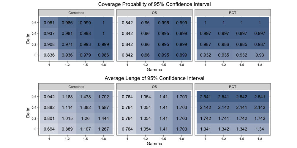
Figure 2: Coverage rates and average lengths for confidence intervals with various combinations of sensitivity parameters, estimated based on 1000 repetitions. The data are generated with $N=1000,\Delta^{\star}=0.2,\Gamma^{\star}=1.2$, and a majority overlap between RCT and OS’s covariate supports.

The results are summarized in Figure 2. We can observe that with any fixed $\Delta$, the RCT confidence intervals have similar coverage probabilities and average length when $\Gamma$, which is specific to the OS, varies, but the OS confidence intervals have higher coverage probabilities and average length as $\Gamma$ increases. Similarly, with any fixed $\Gamma$, the OS confidence intervals have similar coverage probabilities and average length when $\Delta$, which is specific to the RCT, varies, but the RCT confidence intervals have higher coverage probabilities and average as $\Delta$ increases. When either sensitivity parameter increases, the combined intervals improve the coverage probabilities with a wider confidence interval.

It is of interest to compare the coverage rates and average lengths of the combined confidence intervals to that of the confidence intervals from a single data source. When both sensitivity parameters are larger than the true values, $\Delta\geq\Delta^{\star}=0.2$ and $\Gamma\geq\Gamma^{\star}=1.2$, all three intervals have coverage rates above 95%. But, the combined interval has robust performances unless both $\Gamma<\Gamma^{\star}=1.2$ and $\Delta<\Delta^{\star}=.2$, while the OS intervals consistently undercover if $\Gamma<\Gamma^{\star}=1.2$, irrespective of the $\Delta$ values and the RCT intervals consistently undercover if $\Delta<\Delta^{\star}=.2$, irrespective of the $\Gamma$ values. At the same time, the average length of the combined interval tends to be comparable or even shorter than the individual intervals when both sensitivity parameters are larger than the true values. Thus, it is generally safer to use the combined interval than either of the two data sources alone and preferable to use the combined interval than the worst performing of the single data sources.

Power of Sensitivity Analysis

Aiming to evaluate the statistical power of the three inferential methods, we consider the same model as introduced at the beginning of the section with no bias ($\Delta^{\star}=0$ and $\Gamma^{\star}=1$) and varying the treatment effect from $0,0.2,0.4,0.6,0.8$, and $1$, so that the potential outcome under treatment is, $Y(1)=Y(0)+\tau$ for $\tau=0,0.2,0.4,0.6,0.8$ or $1$. We study the power of the proposed method with various choices of sensitivity parameters for the analysis, $\Delta=0,0.2,0.4,0.6$ and $\Gamma=1,1.2,1.5,1.8$. The results in Figure 3 show that the combined method can control the Type I error well in all cases. As $\Gamma$ increases, the power of using OS alone drops; as $\Delta$ increases, the power of using RCT alone drops; but the combined method keeps robust performance.

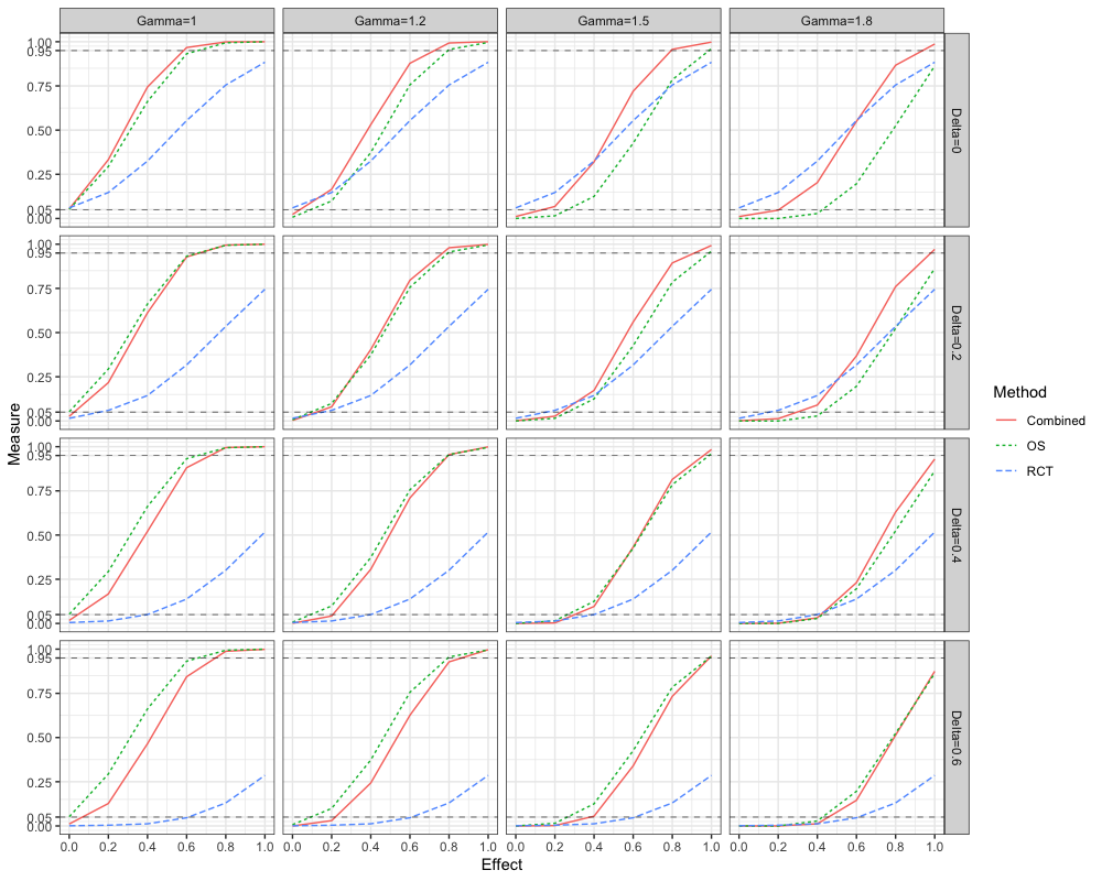
Figure 3: Simulated power curves for the RCT, OS, and the combined method when there is no bias: $\Delta^{\star}=0,\Gamma^{\star}=1$. Total sample size $N=1000$ and majority overlap between the RCT and OS’s covariate supports.

Analysis of CNPRC Primate Dataset

We now return to the CNPRC primate dataset to investigate the effects of lactation on postpartum obesity. Recall that the RCT includes 18 monkeys stratified into 6 matched sets. Each matched set has one treated unit (no lactation) and two control units, matched on several factors: parity, age, weight ($+/-1$ kg), and lactation history. In the OS, there are 231 treated monkeys and 360 control monkeys, and covariate data on age, parity, and baseline weight prior to pregnancy.

To leverage the strengths of both the RCT and the OS, we first apply the proposed matching method that accounts for generalization scores. Specifically, we constructed matched sets consisting of one observational treated unit, one observational control unit, and zero or one copy of an RCT unit. Table 2 shows the covariate balances in terms of absolute standardized mean differences before and after matching, with a noticeable reduction after matching, indicating improved covariate balance across the groups.

We estimated the average treatment effect on the observational treated group using the residuals after covariate adjustment to further adjust the residual imbalances. The results, summarized in Table 3, suggest that, lactation has a modest positive effect on three months postpartum maternal weight. Specifically, we are 95% confident that lactation increases maternal weight by between 0.09 kg and 0.44 kg. These results appear to be robust, even when accounting for a small generalization bias in the RCT ($\Delta=0.02$) and a moderate hidden bias due to unmeasured confounders in the OS ($\Gamma=1.25$). However, lactation has no significant effect on six months postpartum maternal weight. For comparison, the RCT data alone did not yield statistically significant results, likely due to the limited sample size. While the OS data alone led to the same conclusion as the combined analysis, the results were more sensitive to bias, with $\Gamma=1.23$.

In summary, our analysis of the CNPRC primate data supports the conclusion that lactation leads to a modest increase in maternal weight three months postpartum, but no significant effect is observed at six months. The initial weight gain may be attributed to various physiological factors associated with lactation, such as hormonal changes and caloric retention. However, as lactation progresses, increased maternal energy expenditure, along with other factors such as dietary adjustments, physical activity, and metabolic adaptations, could offset the initial weight gain. This may explain the absence of significant weight differences at six months postpartum. These findings, however, contrast with some prior human research, which suggests that breastfeeding is associated with a reduction in postpartum weight retention at six months or longer [Baker et al., 2008, Hebeisen et al., 2024, Loy et al., 2024]. While we do not find any significant weight reduction, one possible explanation for the suggested weight gain is that breastfeeding could reduce visceral adiposity [McClure et al., 2011, 2012]. To further investigate this hypothesis, future studies, including large-scale RCTs, are needed to verify these conjectures.

Table 2: Covariate balance before and after matching: Covariate means and standardized mean differences.

Overlapping Domain: Covariate Mean
	Before Matching				After Matching
	OS		OS		OS		OS
	Treated	RCT	Control		Treated	RCT	Control
Age	6.91	6.92	6.77		6.91	6.39	6.74
Parity	2.62	3.83	2.59		2.62	3.04	2.58
Pre-pregnancy weight	7.38	7.98	7.60		7.38	7.26	7.49
Overlapping Domain: Absolute Standardized Mean Differences
	Before Matching				After Matching
	OS	OS	OS Treated		OS	OS	OS Treated
	Treated – RCT	Control – RCT	– OS Control		Treated – RCT	Control – RCT	– OS Control
Age	0.00	0.05	0.05		0.19	0.12	0.06
Parity	0.60	0.62	0.01		0.21	0.23	0.02
Pre-pregnancy weight	0.35	0.22	0.13		0.07	0.13	0.06
Non-overlapping Domain: Covariate Mean
	Before Matching				After Matching
	OS		OS		OS		OS
	Treated	RCT	Control		Treated	RCT	Control
Age	7.24	-	6.11		7.24	-	7.16
Parity	1.99	-	1.65		1.99	-	2.20
Pre-pregnancy weight	7.37	-	7.15		7.37	-	7.47
Non-overlapping Domain: Absolute Standardized Mean Differences
	Before Matching				After Matching
	OS	OS	OS Treated		OS	OS	OS Treated
	Treated – RCT	Control – RCT	– OS Control		Treated – RCT	Control – RCT	– OS Control
Age	-	-	0.40		-	-	0.03
Parity	-	-	0.17		-	-	0.10
Pre-pregnancy weight	-	-	0.13		-	-	0.06

Table 3: 95% confidence intervals for the effect of lactation

6-month postpartum weight
RCT	$\Delta=0$	$[-0.49,0.54]$
OS	$\Gamma=1$	$[-0.24,0.05]$
Combined	$\Delta=0,\Gamma=1$	$[-0.25,0.08]$
3-month postpartum weight
RCT	$\Delta=0$	$[-1.40,0.25]$
OS	$\Gamma=1$	$[-0.40,-0.10]$
OS	$\Gamma=1.23$	$[-0.49,-0.00]$
Combined	$\Delta=0,\Gamma=1$	$[-0.44,-0.09]$
Combined	$\Delta=0.02,\Gamma=1.25$	$[-0.54,-0.00]$

Supplementary Materials

Details of the Sensitivity Analysis of the Observational Study

Equivalent Form of Rosenbaum’s Sensitivity Model

Rosenbaum’s sensitivity model specification (2) may be equivalently written in the following semiparametric model. Following, Rosenbaum [2020], define principal unobserved covariate $\Pr(Z^{o}_{i}=1\mid Y_{i}^{o}(1),Y^{o}_{i}(0),X^{o}_{i})=:v^{o}_{i}\in[0,1]$, so that treatment assignment is always ignorable (or unconfounded) given $(X^{o}_{i},v^{o}_{i})$. Then, Proposition 12 of Rosenbaum [2002] shows that for some function $\varphi_{x}(v^{o}_{i}):=u^{o}_{i}\in[0,1]$,

$$\Pr(Z_{i}^{o}=1\mid Y_{i}^{o}(1),Y^{o}_{i}(0),X^{o}_{i}=x,v^{o}_{i})=\frac{\exp\{\kappa(x)+\log(\Gamma)u^{o}_{i}\}}{1+\exp\{\kappa(x)+\log(\Gamma)u^{o}_{i}\}},$$ (S1.1)

where $\kappa$ is some unknown function $\kappa$ that depends of the potential outcomes. This model clarifies the role of $\Gamma$, appearing in the coefficient of $u_{i}^{o}$, as encoding the effect of the unmeasured confounder.

Calculation of the Separable Approximation of the Extreme $p$-values

We give the details of the calculation of the separable approximation of the extreme treatment assignment probabilities $\widetilde{\boldsymbol{\eta}}_{i}^{(\beta_{0}^{\star})}$s described in Section 4.1. Fix $\beta_{0}^{\star}$. Define $\tilde{Y}^{o}_{ij}={Y}^{o}_{ij}-\beta_{0}^{\star}Z_{ij}^{o}$ as the adjusted outcomes. Let $\tilde{Y}^{o}_{i(1)}\leq\cdots\leq\tilde{Y}^{o}_{i(J_{i})}$ be the sorted values of the adjusted outcomes. From here onwards let $(1),\ldots,(J_{i})$ denote the indices that give the ordered adjusted outcomes. Consider the set of $(J_{i}-1)$ vectors $\mathcal{P}$ of $\boldsymbol{\eta}_{i}=(\eta_{i(1)},\ldots,\eta_{i(J_{i})})$ where $\eta_{i(1)}=\cdots=\eta_{i(m)}=1/(m+((J_{i}-m)*\Gamma)$ and $\eta_{i(m+1)}=\cdots=\eta_{i(J_{i})}=\Gamma/(m+((J_{i}-m)*\Gamma)$ for $m=1,\ldots,J_{i}-1$. For each $\boldsymbol{\eta}_{i}\in\mathcal{P}$, calculate $\mu(\boldsymbol{\eta}_{i})=\sum_{j=1}^{J_{i}}\tilde{Y}^{o}_{i(j)}\eta_{i(j)}$ and $\sigma^{2}(\boldsymbol{\eta}_{i})=\sum_{j=1}^{J_{i}}\{\tilde{Y}^{o}_{i(j)}\}^{2}\eta_{i(j)}-\mu(\boldsymbol{\eta}_{i})^{2}$.

Search for $\boldsymbol{\eta}_{i}$s in $\mathcal{P}$ that maximizes $\mu(\boldsymbol{\eta}_{i})$. If there are multiple such vectors that maximize these means, choose the one among this set that maximizes $\sigma^{2}(\boldsymbol{\eta}_{i})$. This choice of $\boldsymbol{\eta}_{i}$ gives our separable approximation probabilities $\widetilde{\boldsymbol{\eta}}_{i}^{(\beta_{0}^{\star})}$s.

Confidence Interval Construction

We use numerical methods to find the confidence interval by converting the test for the OS. The process will proceed by first fixing the desired confidence level $\alpha$. Then a root finding method finds the limit of the upper-sided confidence interval $[\beta_{L}^{o},\infty)$, that solves for (3) of the main text, with equality in place of the inequality, when we write $\beta_{L}^{o}$ in place of $\beta_{0}^{\star}$; the subscript $L$ emphasizes that it is the lower limit of the interval. Similarly, a root finding method solves for limit of the lower-sided confidence interval, $(-\infty,\beta_{U}^{o}]$, that solves for (4) in the main text, with equality in place of the inequality, when we write $\beta_{U}^{o}$ in place of $\beta_{0}^{\star}$; the subscript $U$ emphasizes that it is the upper limit of the interval. Most statistical software including R provides a root finding tool, e.g., the uniroot function in R.

Details of the Combined Analysis

The critical level $\kappa_{\alpha}$ follows from the fact that negative two times the logarithm of the product of two independent uniform random variables on $(0,1)$ has a $\chi^{2}$ distribution with $4$ degrees of freedom. Thus, if $p^{o}_{\beta_{0}^{\star}}$ and $p^{r}_{\beta_{0}^{\star}}$ were uniformly distributed under the null, after some calculations, we would get the cutoff $\kappa_{\alpha}=\exp(-\chi^{2}_{4;1-\alpha}/2)$ for the test statistic $p^{o}_{\beta_{0}^{\star}}\times p^{r}_{\beta_{0}^{\star}}$.

Table S1: Covariate balance: Average maximum absolute standardized mean differences in the overlapping domain and nonoverlapping domain, over 500 simulations.

		Maximum Absolute Standardized Mean Differences: $N=500$
		All overlap			Majority overlap						Limited overlap
		Overlap			Overlap			Non-overlap			Overlap			Non-overlap
		Before	After		Before	After		Before	After		Before	After		Before	After
$\Delta=0$	$\Gamma=1$	0.55	0.26		0.51	0.27		0.53	0.30		0.58	0.34		0.34	0.15
$\Delta=0$	$\Gamma=1.2$	0.55	0.26		0.51	0.26		0.53	0.31		0.58	0.34		0.34	0.15
$\Delta=0$	$\Gamma=1.5$	0.54	0.25		0.50	0.25		0.51	0.30		0.56	0.33		0.34	0.15
$\Delta=0.2$	$\Gamma=1$	0.55	0.26		0.51	0.27		0.53	0.30		0.58	0.34		0.34	0.15
$\Delta=0.2$	$\Gamma=1.2$	0.55	0.26		0.51	0.26		0.53	0.31		0.58	0.34		0.34	0.15
$\Delta=0.2$	$\Gamma=1.5$	0.54	0.25		0.50	0.25		0.51	0.30		0.56	0.33		0.34	0.15
$\Delta=0.5$	$\Gamma=1$	0.55	0.26		0.51	0.27		0.53	0.30		0.58	0.34		0.34	0.15
$\Delta=0.5$	$\Gamma=1.2$	0.55	0.26		0.51	0.26		0.53	0.31		0.58	0.34		0.34	0.15
$\Delta=0.5$	$\Gamma=1.5$	0.54	0.25		0.50	0.25		0.51	0.30		0.56	0.33		0.34	0.15
		Maximum Absolute Standardized Mean Differences: $N=1000$
		All overlap			Majority overlap						Limited overlap
		Overlap			Overlap			Non-overlap			Overlap			Non-overlap
		Before	After		Before	After		Before	After		Before	After		Before	After
$\Delta=0$	$\Gamma=1$	0.48	0.18		0.44	0.18		0.40	0.19		0.47	0.23		0.28	0.10
$\Delta=0$	$\Gamma=1.2$	0.48	0.18		0.44	0.18		0.40	0.19		0.47	0.23		0.28	0.10
$\Delta=0$	$\Gamma=1.5$	0.47	0.17		0.43	0.17		0.39	0.19		0.46	0.22		0.27	0.10
$\Delta=0.2$	$\Gamma=1$	0.48	0.18		0.44	0.18		0.40	0.19		0.47	0.23		0.28	0.10
$\Delta=0.2$	$\Gamma=1.2$	0.48	0.18		0.44	0.18		0.40	0.19		0.47	0.23		0.28	0.10
$\Delta=0.2$	$\Gamma=1.5$	0.47	0.17		0.43	0.17		0.39	0.19		0.46	0.22		0.27	0.10
$\Delta=0.5$	$\Gamma=1$	0.48	0.18		0.44	0.18		0.40	0.19		0.47	0.23		0.28	0.10
$\Delta=0.5$	$\Gamma=1.2$	0.48	0.18		0.44	0.18		0.40	0.19		0.47	0.23		0.28	0.10
$\Delta=0.5$	$\Gamma=1.5$	0.47	0.17		0.43	0.17		0.39	0.19		0.46	0.22		0.27	0.10

Covariate Balance for Simulation Study

To evaluate the match quality for the simulation study in §5.1, we use the maximum absolute standardized mean differences in the overlapping domain and non-overlapping domain and summarize the results in Table S1. We can observe that our matching procedure greatly reduces the large standardized mean differences in all cases. The match quality improves as the sample size increases.

Proofs of the Technical Results

Proof of Theorem 1.

Let $\tau_{ij}=Y_{ij}^{o}(1)-Y_{ij}^{o}(0)$.

Assumption S1.

* $\tau_{ij}\geq-M$ for some constant $M$.

* The strata are independent across.

* $\frac{2}{I^{2}}\sum_{i}\sum_{j}Y_{ij}^{o}(0)^{2}+\frac{2}{I^{2}}\sum_{i}\sum_{j}\tau_{ij}^{2}\rightarrow 0$ almost surely.

* $\frac{1}{I^{2}}\sum_{i}Var(\hat{\tau}_{i}^{2})\rightarrow 0$, $\lim_{I\rightarrow\infty}\frac{1}{I}\sum_{i}E(\hat{\tau}_{i})<\infty$, $\lim_{I\rightarrow\infty}\frac{1}{I}\sum_{i}Var(\hat{\tau}_{i})\in(0,\infty)$, and $\lim_{I\rightarrow\infty}\frac{1}{I}\sum_{i}(\hat{\tau}_{i}-E\hat{\tau}_{i})^{2}$ converges almost surely to a random variable with finite expectation.

Note: $\lim_{I\rightarrow\infty}\frac{1}{I}\sum_{i}E(\hat{\tau}_{i})<\infty$ is implied by an assumption $\lim_{I\rightarrow\infty}\frac{1}{I}\sum_{i}\sum_{j}E|Y_{ij}^{o}|<\infty$.

$\lim_{I\rightarrow\infty}\frac{1}{I}\sum_{i}Var(\hat{\tau}_{i})\in(0,\infty)$ is implied by an assumption $\lim_{I\rightarrow\infty}\frac{1}{I}\sum_{i}J_{i}E({Y_{ij}^{o}}^{2})\in(0,\infty)$.

$\frac{1}{I^{2}}\sum_{i}Var(\hat{\tau}_{i}^{2})\rightarrow 0$ is implied by an assumption $\lim_{I\rightarrow\infty}\frac{1}{I^{2}}\sum_{i}J_{i}^{3}\sum_{j}E{Y_{ij}^{o}}^{4}=0$.

Using Kolmogorov’s SLLN, if $\lim_{I\rightarrow\infty}\sum_{i}\frac{J_{i}^{3}}{i^{2}}\sum_{j}E{Y_{ij}^{o}}^{4}<\infty$ and $\lim_{I\rightarrow\infty}\frac{1}{I}\sum_{i}J_{i}E({Y_{ij}^{o}}^{2})<\infty$, we have the final assumption that $\lim_{I\rightarrow\infty}\frac{1}{I}\sum_{i}(\hat{\tau}_{i}-E\hat{\tau}_{i})^{2}$ converges almost surely to a random variable with finite expectation.

—————————

The $\tilde{\tau}_{i}$ statistic is unchanged if we redefine $Y_{ij}^{o}=Y_{ij}^{o}+MZ_{ij}^{o}$ and $\beta_{0}^{\star}=\beta_{0}^{\star}+M$. Thus, without loss of generality assume $\tau_{ij}\geq 0$ and $\beta_{0}^{\star}\geq 0$. To simplify the notation write $\tilde{\tau}_{i}^{(\beta_{0}^{\star})}$ as $\tilde{\tau}_{i}$.

We first show that

$$\Pr\left\{I\times se^{2}\left(\frac{1}{I}\sum_{i}\tilde{\tau}_{i}\right)\geq\frac{1}{I}Var\left(\sum_{i}\tilde{\tau}_{i}\right)\right\}\rightarrow 1.$$

See that $I\times se^{2}\left(\frac{1}{I}\sum_{i}\tilde{\tau}_{i}\right)=\frac{1}{I-1}\sum_{i}(\tilde{\tau}_{i}-\bar{\tilde{\tau}})^{2}$. Also, $Var(\sum_{i}\tilde{\tau}_{i})=\sum_{i}\{E(\tilde{\tau}_{i}^{2})-[E\tilde{\tau}_{i}]^{2}\}$. Thus,

$$I\times se^{2}\left(\frac{1}{I}\sum_{i}\tilde{\tau}_{i}\right)-\frac{1}{I}Var\left(\sum_{i}\tilde{\tau}_{i}\right)$$

$$= \frac{1}{I-1}\sum_{i}\tilde{\tau}_{i}^{2}-\frac{I}{I-1}\bar{\tilde{\tau}}^{2}-\frac{1}{I}\sum_{i}\{E(\tilde{\tau}_{i}^{2})-[E\tilde{\tau}_{i}]^{2}\}$$

$$\geq \frac{1}{I-1}\sum_{i}(\tilde{\tau}_{i}^{2}-E\tilde{\tau}_{i}^{2})-\frac{I}{I-1}(\bar{\tilde{\tau}}^{2}-(\frac{1}{I}\sum_{i}E\tilde{\tau}_{i})^{2})-\frac{I}{I-1}(\frac{1}{I}\sum_{i}E\tilde{\tau}_{i})^{2}+\frac{1}{I}\sum_{i}[E\tilde{\tau}_{i}]^{2}$$

$$\geq \frac{1}{I-1}\sum_{i}(\tilde{\tau}_{i}^{2}-E\tilde{\tau}_{i}^{2})-\frac{I}{I-1}(\bar{\tilde{\tau}}^{2}-(\frac{1}{I}\sum_{i}E\tilde{\tau}_{i})^{2})+\left\{1-\frac{I}{I-1}\right\}(\frac{1}{I}\sum_{i}E\tilde{\tau}_{i})^{2}.$$

It suffices to show that the three terms go to 0 in probability. The last term is obvious. For the first two terms, use Chebyshev’s inequality. Since they have mean zero, it suffices to show that the variances of the terms go to zero as $I$ goes to infinity.

For the first term,

$$Var\left\{\frac{1}{I-1}\sum_{i}(\tilde{\tau}_{i}^{2}-E\tilde{\tau}_{i}^{2})\right\}\leq\frac{1}{(I-1)^{2}}\sum_{i}Var(\tilde{\tau}_{i}^{2}).$$

Similarly, for the second term,

$$Var\left(\bar{\tilde{\tau}}^{2}\right)$$

$$= \frac{1}{I^{2}}Var\left\{\left(\sum_{i}\tilde{\tau}_{i}\right)^{2}\right\}$$

$$= \frac{1}{I^{2}}\sum_{i}E\tilde{\tau}_{i}^{2}+\frac{1}{I^{2}}\sum_{i\neq j}E\tilde{\tau}_{i}E\tilde{\tau}_{j}-\frac{1}{I^{2}}\left[E\sum_{i}\tilde{\tau}_{i}\right]^{2}$$

$$= \frac{1}{I^{2}}\sum_{i}E\tilde{\tau}_{i}^{2}+\frac{1}{I^{2}}\left[\sum_{i}E\tilde{\tau}_{i}\right]^{2}-\frac{1}{I^{2}}\left(\sum_{i}E\tilde{\tau}_{i}\right)^{2}-\frac{1}{I^{2}}\left[E\sum_{i}\tilde{\tau}_{i}\right]^{2}$$

$$= \frac{1}{I^{2}}\sum_{i}E\tilde{\tau}_{i}^{2}-\frac{1}{I^{2}}\left(\sum_{i}E\tilde{\tau}_{i}\right)^{2}=\frac{1}{I^{2}}\sum_{i}Var(\tilde{\tau}_{i}).$$

Thus, we have proved as $I\rightarrow\infty$

$$\Pr\left\{I\times se^{2}\left(\frac{1}{I}\sum_{i}\tilde{\tau}_{i}\right)\geq\frac{1}{I}Var\left(\sum_{i}\tilde{\tau}_{i}\right)\right\}\rightarrow 1.$$

Next, we show that $\tilde{\tau}_{i}^{(\beta_{0}^{\star})}\leq 0$. We simplify the notation to write $\widetilde{\eta}_{ij}^{(\beta_{0}^{\star})}$ as $\eta_{ij}$.

Recall $\hat{\tau_{i}}$

$$\hat{\tau_{i}}=\sum_{j}Z_{ij}^{o}(Y_{ij}^{o}-Z_{ij}^{o}\beta_{0}^{\star})-\frac{1}{J_{i}-1}\sum_{j}(1-Z_{ij}^{o})(Y_{ij}^{o}-Z_{ij}^{o}\beta_{0}^{\star}),$$

and

$$\overline{\hat{\tau}}=\frac{1}{I}\sum_{i}c_{i}\hat{\tau}_{i}.$$

For our purpose $c_{i}=1$ throughout, but one may choose some other coefficients, e.g., $c_{i}=1/J_{i}$.

Some calculations show

$$\overline{\hat{\tau}}=\frac{1}{I}\sum_{i}c_{i}\sum_{j}Y_{ij}^{o}(0)Z_{ij}^{o}\frac{J_{i}}{J_{i}-1}-\frac{1}{I}\sum_{i}c_{i}\frac{1}{J_{i}-1}\sum_{j}Y_{ij}^{o}(0)-\beta_{0}^{\star}\bar{c}+\frac{1}{I}\sum_{i}c_{i}\sum_{j}Z_{ij}^{o}\tau_{ij}.$$

Let

$$E_{\tau}=\frac{1}{I}\sum_{i}c_{i}\sum_{j}Y_{ij}^{o}(0)\eta_{ij}\frac{J_{i}}{J_{i}-1}-\frac{1}{I}\sum_{i}c_{i}\frac{1}{J_{i}-1}\sum_{j}Y_{ij}^{o}(0)-\beta\bar{c}+\frac{1}{I}\sum_{i}c_{i}\sum_{j}\eta_{ij}\tau_{ij}.$$

Subtracting the two,

$$\overline{\hat{\tau}}-E_{\tau}=\frac{1}{I}\sum_{i}c_{i}\sum_{j}Y_{ij}^{o}(0)(Z_{ij}^{o}-\eta_{ij})\frac{J_{i}}{J_{i}-1}+\frac{1}{I}\sum_{i}c_{i}\sum_{j}(Z_{ij}^{o}-\eta_{ij})\tau_{ij}.$$

Let $\eta^{\prime}_{ij}=E(Z_{ij}^{o}\mid\mathcal{F})$.

Let’s use Chebyshev to say that we can approximate the above $\overline{\tilde{\tau}}-E_{\tau}$ by

$$\frac{1}{I}\sum_{i}c_{i}\sum_{j}Y_{ij}^{o}(0)(\eta^{\prime}_{ij}-\eta_{ij})\frac{J_{i}}{J_{i}-1}+\frac{1}{I}\sum_{i}c_{i}\sum_{j}(\eta^{\prime}_{ij}-\eta_{ij})\tau_{ij}.$$

The approximation follows since

$$Var\{\overline{\hat{\tau}}-E_{\tau}\mid\mathcal{F}\}$$

$$\leq\frac{1}{I^{2}}\sum_{i}\frac{c_{i}^{2}}{(J_{i}-1)^{2}}\sum_{j}(J_{i}Y_{ij}^{o}(0)+(J_{i}-1)\tau_{ij})^{2}\eta^{\prime}_{ij}(1-\eta^{\prime}_{ij})$$

$$\leq\frac{1}{I^{2}}\sum_{i}\frac{c_{i}^{2}}{(J_{i}-1)^{2}}\sum_{j}2(J_{i}^{2}Y_{ij}^{o}(0)^{2}+(J_{i}-1)^{2}\tau_{ij}^{2})\frac{1}{4}$$

$$\leq\frac{2}{I^{2}}\sum_{i}c_{i}^{2}\sum_{j}Y_{ij}^{o}(0)^{2}+\frac{2}{I^{2}}\sum_{i}c_{i}^{2}\sum_{j}\tau_{ij}^{2}\rightarrow 0.$$

The limit follows from our assumptions.

Since $\eta_{ij}$ maximizes $E(\bar{\hat{\tau}})$ for large enough $I$, (S4) is less than or equal to 0. Thus, we have with probability going to 1, $\overline{\hat{\tau}}-E_{\tau}\leq 0$.

However, $E_{\tau}$ cannot be calculated from the observed data. Consider instead,

$$E_{\tau}^{\prime}=\frac{1}{I}\sum_{i}c_{i}\sum_{j}\eta_{ij}(Y_{ij}^{o}-Z_{ij}^{o}\beta)-\frac{1}{I}\sum_{i}c_{i}\frac{1}{J_{i}-1}\sum_{j}(1-\eta_{ij})(Y_{ij}^{o}-Z_{ij}^{o}\beta_{0}^{\star}).$$

$$E_{\tau}^{\prime} =\frac{1}{I}\sum_{i}c_{i}\sum_{j}\eta_{ij}(Y_{ij}^{o}-Z_{ij}^{o}\beta_{0}^{\star})-\frac{1}{I}\sum_{i}c_{i}\frac{1}{J_{i}-1}\sum_{j}(1-\eta_{ij})(Y_{ij}^{o}-Z_{ij}^{o}\beta_{0}^{\star})$$

$$=\frac{1}{I}\sum_{i}c_{i}\left\{\sum_{j}\eta_{ij}Z_{ij}^{o}(\tau_{ij}-\beta_{0}^{\star})+\sum_{j}\eta_{ij}Y_{ij}^{o}(0)-\frac{1}{J_{i}-1}\sum_{j}(1-\eta_{ij})Z_{ij}^{o}(\tau_{ij}-\beta_{0}^{\star})\right.$$

$$\ \ \ \left.-\frac{1}{J_{i}-1}\sum_{j}(1-\eta_{ij})Y_{ij}^{o}(0)\right\}$$

Thus,

$$E_{\tau}-E_{\tau}^{\prime} =-\beta_{0}^{\star}\bar{c}+\frac{1}{I}\sum_{i}c_{i}\sum_{j}\eta_{ij}\tau_{ij}-\frac{1}{I}\sum_{i}c_{i}\sum_{j}\eta_{ij}(\tau_{ij}-Z_{ij}^{o}\beta_{0}^{\star})+\frac{1}{I}\sum_{i}c_{i}\frac{1}{J_{i}-1}\sum_{j}(1-\eta_{ij})Z_{ij}^{o}(\tau_{ij}-\beta_{0}^{\star})$$

$$=-\beta_{0}^{\star}\bar{c}-\frac{1}{I}\sum_{i}c_{i}\frac{1}{J_{i}-1}\sum_{j}\tau_{ij}(1-\eta_{ij})Z_{ij}^{o}+\beta_{0}^{\star}\frac{1}{I}\sum_{i}c_{i}\sum_{j}\{1-(1-\eta_{ij})/(J_{i}-1)\}Z_{ij}^{o}$$

$$=-\beta_{0}^{\star}\bar{c}+\beta_{0}^{\star}\frac{1}{I}\sum_{i}c_{i}\{1-1/(J_{i}-1)+\sum_{j}\eta_{ij}Z_{ij}^{o}/(J_{i}-1)\}-\frac{1}{I}\sum_{i}c_{i}\frac{1}{J_{i}-1}\sum_{j}\tau_{ij}(1-\eta_{ij})Z_{ij}^{o}$$

$$=-\beta_{0}^{\star}\frac{1}{I}\sum_{i}c_{i}/(J_{i}-1)+\beta_{0}^{\star}\frac{1}{I}\sum_{i}c_{i}/(J_{i}-1)\sum_{j}\eta_{ij}Z_{ij}^{o}-\frac{1}{I}\sum_{i}c_{i}\frac{1}{J_{i}-1}\sum_{j}\tau_{ij}(1-\eta_{ij})Z_{ij}^{o}$$

$$\leq-\beta_{0}^{\star}\frac{1}{I}\sum_{i}c_{i}/(J_{i}-1)+\beta_{0}^{\star}\frac{1}{I}\sum_{i}c_{i}/(J_{i}-1)$$

$$\quad\quad\text{since, }\sum_{j}Z_{ij}^{o}\eta_{ij}\leq\sqrt{\sum_{j}(Z_{ij}^{o})^{2}}\sqrt{\sum_{j}\eta_{ij}^{2}}\leq\sqrt{\sum_{j}Z_{ij}^{o}}\sqrt{\sum_{j}\eta_{ij}}=1$$

$$=0.$$

In the above we have used that $\tau_{ij}\geq 0$ and $\beta_{0}^{\star}\geq 0$.

Thus, with probability going to 1,

$$\overline{\hat{\tau}}-E_{\tau}^{\prime}=\overline{\hat{\tau}}-E_{\tau}+E_{\tau}-E_{\tau}^{\prime}\leq 0.$$

Putting things together, with probability going to 1,

$$\overline{\hat{\tau}}-E_{\tau}^{\prime}\leq\overline{\hat{\tau}}-E(\overline{\hat{\tau}})$$

$$\Rightarrow \frac{\overline{\hat{\tau}}-E_{\tau}^{\prime}}{\{Var(\frac{1}{I}\sum_{i}\tilde{\tau}_{i})\}^{1/2}}\leq\frac{\overline{\hat{\tau}}-E(\overline{\hat{\tau}})}{\{Var(\frac{1}{I}\sum_{i}\tilde{\tau}_{i})\}^{1/2}}$$

$$\Rightarrow \frac{\overline{\hat{\tau}}-E_{\tau}^{\prime}}{se\left(\frac{1}{I}\sum_{i}\tilde{\tau}_{i}\right)}\frac{se\left(\frac{1}{I}\sum_{i}\tilde{\tau}_{i}\right)}{\{Var(\frac{1}{I}\sum_{i}\tilde{\tau}_{i})\}^{1/2}}\leq\frac{\overline{\hat{\tau}}-E(\overline{\hat{\tau}})}{\{Var(\frac{1}{I}\sum_{i}\tilde{\tau}_{i})\}^{1/2}}.$$

Note, $\tilde{\tau}_{i}=\hat{\tau}_{i}-\left\{\sum_{j}\eta_{ij}(Y_{ij}^{o}-Z_{ij}^{o}\beta_{0}^{\star})-\frac{1}{J_{i}-1}\sum_{j}(1-\eta_{ij})(Y_{ij}^{o}-Z_{ij}^{o}\beta_{0}^{\star})\right\}$. Recall, $c_{i}=1$ for all $i$; so, $\overline{\hat{\tau}}=\frac{1}{I}\sum_{i}\hat{\tau}_{i}$, and $E_{\tau}^{\prime}=\frac{1}{I}\sum_{i}\left\{\sum_{j}\eta_{ij}(Y_{ij}^{o}-Z_{ij}^{o}\beta_{0}^{\star})-\frac{1}{J_{i}-1}\sum_{j}(1-\eta_{ij})(Y_{ij}^{o}-Z_{ij}^{o}\beta_{0}^{\star})\right\}$. So, $\frac{1}{I}\sum_{i}\tilde{\tau}_{i}=\overline{\hat{\tau}}-E_{\tau}^{\prime}$.

Take $t\geq 0$.

$$\Pr\left\{\frac{\overline{\hat{\tau}}-E_{\tau}^{\prime}}{se\left(\frac{1}{I}\sum_{i}\tilde{\tau}_{i}\right)}\geq t\right\}$$

$$= \Pr\left\{\frac{\overline{\hat{\tau}}-E_{\tau}^{\prime}}{se\left(\frac{1}{I}\sum_{i}\tilde{\tau}_{i}\right)}\frac{se\left(\frac{1}{I}\sum_{i}\tilde{\tau}_{i}\right)}{\{Var(\frac{1}{I}\sum_{i}\tilde{\tau}_{i})\}^{1/2}}\geq t\frac{se\left(\frac{1}{I}\sum_{i}\tilde{\tau}_{i}\right)}{\{Var(\frac{1}{I}\sum_{i}\tilde{\tau}_{i})\}^{1/2}}\right\}$$

$$\leq \Pr\left\{\frac{\overline{\hat{\tau}}-E(\overline{\hat{\tau}})}{\{Var(\frac{1}{I}\sum_{i}\tilde{\tau}_{i})\}^{1/2}}\geq t\frac{se\left(\frac{1}{I}\sum_{i}\tilde{\tau}_{i}\right)}{\{Var(\frac{1}{I}\sum_{i}\tilde{\tau}_{i})\}^{1/2}}\mid A_{I}^{c}\right\}\Pr(A_{I}^{c})+\Pr(A_{I})$$

$$\leq \Pr\left\{\frac{\overline{\hat{\tau}}-E(\overline{\hat{\tau}})}{\{Var(\frac{1}{I}\sum_{i}\tilde{\tau}_{i})\}^{1/2}}\geq t\mid A_{I}^{c},B_{I}^{c}\right\}\Pr(A_{I}^{c})\Pr(B_{I}^{c})+\Pr(A_{I})+\Pr(B_{I}).$$

Where $A_{I}=\{\overline{\hat{\tau}}-E_{\tau}^{\prime}>0\}$ and $B_{I}=\{{se\left(\frac{1}{I}\sum_{i}\tilde{\tau}_{i}\right)}<{\{Var(\frac{1}{I}\sum_{i}\tilde{\tau}_{i})\}^{1/2}}\}$; $A_{I}^{c}$, $B_{I}^{c}$ are complements of these events. Note $\Pr(A_{I})\rightarrow 0$ and $\Pr(B_{I})\rightarrow 0$. Now,

$$\Pr\left\{\frac{\overline{\hat{\tau}}-E(\overline{\hat{\tau}})}{\{Var(\frac{1}{I}\sum_{i}\tilde{\tau}_{i})\}^{1/2}}\geq t\mid A_{I}^{c},B_{I}^{c}\right\}$$

$$= \Pr\left\{\frac{\overline{\hat{\tau}}-E(\overline{\hat{\tau}})}{\{Var(\frac{1}{I}\sum_{i}\tilde{\tau}_{i})\}^{1/2}}\geq t\right\}$$

$$\quad-\Pr\left\{\frac{\overline{\hat{\tau}}-E(\overline{\hat{\tau}})}{\{Var(\frac{1}{I}\sum_{i}\tilde{\tau}_{i})\}^{1/2}}\geq t\mid A_{I}\text{ or }B_{I}\right\}\Pr(A_{I}\text{ or }B_{I})/\Pr(A_{I}^{c},B_{I}^{c}).$$

Since, $\Pr(A_{I}\text{ or }B_{I})\leq\Pr(A_{I})+\Pr(B_{I})\rightarrow 0$ and $\Pr(A_{I}^{c},B_{I}^{c})\geq\Pr(A_{I}^{c})+\Pr(B_{I}^{c})-1\rightarrow 1$, we have,

$$\lim\sup_{I\rightarrow\infty}\Pr\left\{\frac{\overline{\hat{\tau}}-E_{\tau}^{\prime}}{se\left(\frac{1}{I}\sum_{i}\tilde{\tau}_{i}\right)}\geq t\right\}\leq\lim_{I\rightarrow\infty}\Pr\left\{\frac{\overline{\hat{\tau}}-E(\overline{\hat{\tau}})}{\{Var(\frac{1}{I}\sum_{i}\tilde{\tau}_{i})\}^{1/2}}\geq t\right\}=1-\Phi(t).$$

The last equality is by using Lindeberg’s CLT as we establish below.

Let $\sigma_{i}^{2}=var(\hat{\tau}_{i})$ and $s_{I}^{2}:=\sum_{i}\sigma_{i}^{2}$. By our assumption $\frac{1}{I}s_{I}^{2}$ converges almost surely to a positive number. Thus, $s_{I}\rightarrow\infty$ in probability. Thus, to establish Lindeberg’s condition it is enough to show that

$$\lim_{I\rightarrow\infty}\frac{1}{I}\sum_{i}E\left\{(\hat{\tau}_{i}-E(\hat{\tau}_{i}))^{2}\times I(|\hat{\tau}_{i}-E(\hat{\tau}_{i})|>\epsilon s_{I})\right\}=0.$$

Write

$$\frac{1}{I}\sum_{i}E\left\{(\hat{\tau}_{i}-E(\hat{\tau}_{i}))^{2}\times I(|\hat{\tau}_{i}-E(\hat{\tau}_{i})|>\epsilon s_{I})\right\}=E\left\{\frac{1}{I}\sum_{i}(\hat{\tau}_{i}-E(\hat{\tau}_{i}))^{2}\times I(|\hat{\tau}_{i}-E(\hat{\tau}_{i})|>\epsilon s_{I})\right\}.$$

We want to interchange the limit and expectation. We use a general version of the dominated convergence theorem. We check the conditions using our assumption. First, $\frac{1}{I}\sum_{i}(\hat{\tau}_{i}-E(\hat{\tau}_{i}))^{2}\times I(|\hat{\tau}_{i}-E(\hat{\tau}_{i})|>\epsilon s_{I})\leq\frac{1}{I}\sum_{i}(\hat{\tau}_{i}-E(\hat{\tau}_{i}))^{2}$. Next, $E(\frac{1}{I}\sum_{i}(\hat{\tau}_{i}-E(\hat{\tau}_{i}))^{2})=\frac{1}{I}\sum_{i}var(\hat{\tau}_{i})$. And its limit is finite. Finally, $\frac{1}{I}\sum_{i}(\hat{\tau}_{i}-E(\hat{\tau}_{i}))^{2}$ converges almost surely to a random variable with finite expectation. Then, the general version of the dominated convergence theorem applies.

So, suffices to show $\lim_{I\rightarrow\infty}\frac{1}{I}\sum_{i}(\hat{\tau}_{i}-E(\hat{\tau}_{i}))^{2}\times I(|\hat{\tau}_{i}-E(\hat{\tau}_{i})|>\epsilon s_{I})$ goes to zero almost surely.

To see this note that for any $M>0$, for large enough $I$, $\lim_{I\rightarrow\infty}\frac{1}{I}\sum_{i}(\hat{\tau}_{i}-E(\hat{\tau}_{i}))^{2}\times I(|\hat{\tau}_{i}-E(\hat{\tau}_{i})|>\epsilon s_{I})\leq\lim_{I\rightarrow\infty}\frac{1}{I}\sum_{i}(\hat{\tau}_{i}-E(\hat{\tau}_{i}))^{2}\times I(|\hat{\tau}_{i}-E(\hat{\tau}_{i})|>M).$ Thus, $\lim_{I\rightarrow\infty}\frac{1}{I}\sum_{i}(\hat{\tau}_{i}-E(\hat{\tau}_{i}))^{2}\times I(|\hat{\tau}_{i}-E(\hat{\tau}_{i})|>\epsilon s_{I})\leq\lim_{M\rightarrow\infty}\lim_{I\rightarrow\infty}\frac{1}{I}\sum_{i}(\hat{\tau}_{i}-E(\hat{\tau}_{i}))^{2}\times I(|\hat{\tau}_{i}-E(\hat{\tau}_{i})|>M).$ Since $\frac{1}{I}\sum_{i}(\hat{\tau}_{i}-E(\hat{\tau}_{i}))^{2}\times I(|\hat{\tau}_{i}-E(\hat{\tau}_{i})|>M)$ is monotone in $M$, we can interchange the two limits. Thus, look at $\lim_{I\rightarrow\infty}\lim_{M\rightarrow\infty}\frac{1}{I}\sum_{i}(\hat{\tau}_{i}-E(\hat{\tau}_{i}))^{2}\times I(|\hat{\tau}_{i}-E(\hat{\tau}_{i})|>M)$; which is zero. Thus, we have checked the Lindeberg condition for the CLT of the average of the $\hat{\tau}_{i}$s.

Thus, in the theorem’s original notation, for $t>0$,

$$\lim\sup_{I\rightarrow\infty}\Pr\left\{\frac{\frac{1}{I}\sum_{i}{\tilde{\tau}}_{i}^{(\beta_{0}^{\star})}}{se\left(\frac{1}{I}\sum_{i}\tilde{\tau}_{i}^{(\beta_{0}^{\star})}\right)}\geq t\right\}\leq 1-\Phi(t).$$

Hence we get an asymptotically valid confidence interval for the ATOT. Q.E.D.

Throughout the proofs of Theorems 2 and 3 we refer to the result in the second paragraph of page 279, Section 19.4 of van der Vaart [1998] as the GC class theorem and to Lemma 19.24 (See page 280, Section 19.2) of van der Vaart [1998] as Donsker’s theorem. These may be abuses of nomenclature, as there are other theorems with such names, but they simplifies our presentation.

Proof of Theorem 2.

Write $C_{m}=\hat{\nu}(X_{m})$, where $\hat{\nu}$ is estimated from the data. Notice that by construction $\hat{\nu}(x)=0$ for $x\not\in\mathcal{X}$.

Let $\mathbf{X}=\{X_{m}^{r}:m=1,\ldots,n_{r}\}$.

Assumption S2.

* $\hat{\nu}$ is in a Glivenko-Cantelli (GC) class, $\hat{\nu}(x)\rightarrow\nu(x)$ almost surely for all $x$ and the functions are bounded. Here and later,

$$\nu(x)=\Pr(Z_{l}^{o}=1\mid X_{l}^{o}=x)\times\Pr(S_{k}=0\mid X_{k}=x)/\Pr(S_{k}=1\mid X_{k}=x).$$

* $\max\{\tilde{\theta}_{m},1-\tilde{\theta}_{m}\}\leq\delta_{n_{r}}$ for all $m$. $\delta_{n_{r}}\rightarrow\delta\in(0,1)$.

* $E(Y_{m}^{r}(z)^{2})<\infty$ and $E[E(Y_{m}^{r}(z)\mid X_{m})^{2}]<\infty$ for $z=0,1$.

* Let $\tilde{\theta}_{m,m^{\prime}}=cov(Z_{m}^{r},Z_{m^{\prime}}^{r}\mid\mathbf{X})$. Assume $A_{n_{r}}\subseteq\{1,\ldots,n_{r}\}^{2}$ so that for $m,m^{\prime}\in A_{n_{r}}$, $m\neq m^{\prime}$ and , $\tilde{\theta}_{m,m^{\prime}}\leq g(n_{r})$, for some function $g$ with $g(n_{r})\rightarrow 0$.

*Also, $\frac{1}{n_{r}^{2}}\sum_{m\neq m^{\prime}\not\in A_{n_{r}}}E(|Y_{m}^{r}(1)|+|Y_{m}^{r}(0)|\mid\mathbf{X})E(|Y_{m^{\prime}}^{r}(1)|+|Y_{m^{\prime}}^{r}(0)|\mid\mathbf{X})\rightarrow 0$ almost surely.

* Assume $S_{l}\perp(Y_{l}(1),Y_{l}(0))\mid X_{l}$ and $(Y_{l}(1)-Y_{l}(0))\perp Z_{l}^{o}\mid X_{l},S_{l}=0$.

—————————

Note that $\sum_{m}C_{m}/n_{r}$ converges almost surely to $E(\nu(X_{m}^{r}))$ by GC class theorem and our assumptions. write,

$$\frac{1}{{n_{r}}}\sum_{m}C_{m}\widehat{\beta^{r}_{\chi}}=\frac{1}{{n_{r}}}\sum_{m}C_{m}\left\{\frac{Z^{r}_{m}Y^{r}_{m}}{\tilde{\theta}_{m}}-\frac{(1-Z^{r}_{m})Y^{r}_{m}}{1-\tilde{\theta}_{m}}\right\}.$$

Given covariate data $X$, consider the conditional variance of the term. We show that it goes to zero.

Let $f_{m}:=f(Y_{m}(1),Y_{m}(0))=\frac{Z^{r}_{m}Y^{r}_{m}}{\tilde{\theta}_{m}}-\frac{(1-Z^{r}_{m})Y^{r}_{m}}{1-\tilde{\theta}_{m}}$. Let $\mathbf{X}=\{X_{m}^{r}:m=1,\ldots,n_{r}\}$. Using the fact that $Z_{m}$s are independent of the potential outcomes given the covariates, the variance is

$$\frac{1}{n_{r}^{2}}\sum_{m}C_{m}^{2}\left\{\tilde{\theta}_{m}E(f_{m}^{2}\mid X)-\tilde{\theta}_{m}^{2}[E(f_{m}\mid\mathbf{X})]^{2}\right\}+\frac{1}{n_{r}^{2}}\sum_{m\neq m^{\prime}}C_{m}C_{m^{\prime}}E(f_{m}f_{m^{\prime}}\mid\mathbf{X})\tilde{\theta}_{m,m^{\prime}}$$

$$\leq \frac{K^{2}}{n_{r}^{2}}\sum_{m}\left\{\frac{2}{\delta_{n_{r}}^{2}}E(Y_{m}^{r}(1)^{2}+Y_{m}^{r}(0)^{2}\mid\mathbf{X})+\frac{2}{\delta_{n_{r}}^{2}}[E(|Y_{m}^{r}(1)|\mid X)^{2}+E(|Y_{m}^{r}(0)|\mid\mathbf{X})^{2}]\right\}$$

$$+\frac{K^{2}}{\delta_{n_{r}}^{2}n_{r}^{2}}\sum_{m\neq m^{\prime}}E(|Y_{m}^{r}(1)|+|Y_{m}^{r}(0)|\mid\mathbf{X})E(|Y_{m^{\prime}}^{r}(1)|+|Y_{m^{\prime}}^{r}(0)|\mid\mathbf{X})|\tilde{\theta}_{m,m^{\prime}}|,$$

where $K$ is the upper bound for the $C_{m}$s.

The first term goes to zero by strong law of large number and our finite moment assumptions.

For the second term

$$\frac{K^{2}}{\delta_{n_{r}}^{2}n_{r}^{2}}\sum_{m\neq m^{\prime}}E(|Y_{m}^{r}(1)|+|Y_{m}^{r}(0)|\mid\mathbf{X})E(|Y_{m^{\prime}}^{r}(1)|+|Y_{m^{\prime}}^{r}(0)|\mid\mathbf{X})|\tilde{\theta}_{m,m^{\prime}}|$$

$$\leq \frac{K^{2}g(n_{r})}{\delta_{n_{r}}^{2}n_{r}^{2}}\sum_{m\neq m^{\prime}\in A_{n_{r}}}E(|Y_{m}^{r}(1)|+|Y_{m}^{r}(0)|\mid\mathbf{X})E(|Y_{m^{\prime}}^{r}(1)|+|Y_{m^{\prime}}^{r}(0)|\mid\mathbf{X})$$

$$+\frac{K^{2}\times 1}{\delta_{n_{r}}^{2}n_{r}^{2}}\sum_{m\neq m^{\prime}\not\in A_{n_{r}}}E(|Y_{m}^{r}(1)|+|Y_{m}^{r}(0)|\mid\mathbf{X})E(|Y_{m^{\prime}}^{r}(1)|+|Y_{m^{\prime}}^{r}(0)|\mid\mathbf{X})$$

$$= \frac{K^{2}g(n_{r})}{\delta_{n_{r}}^{2}}\left(\frac{1}{n_{r}}\sum_{m}E(|Y_{m}^{r}(1)|+|Y_{m}^{r}(0)|\mid\mathbf{X})\right)^{2}-\frac{K^{2}g(n_{r})}{\delta_{n_{r}}^{2}n_{r}^{2}}\sum_{m}E(|Y_{m}^{r}(1)|+|Y_{m}^{r}(0)|\mid\mathbf{X})^{2}$$

$$+\frac{K^{2}\times(1-g(n_{r}))}{\delta_{n_{r}}^{2}n_{r}^{2}}\sum_{m\neq m^{\prime}\not\in A_{n_{r}}}E(|Y_{m}^{r}(1)|+|Y_{m}^{r}(0)|\mid\mathbf{X})E(|Y_{m^{\prime}}^{r}(1)|+|Y_{m^{\prime}}^{r}(0)|\mid\mathbf{X}).$$

Use the strong law of large numbers for the averages in thr first and the second terms. Then, by our assumptions, all three terms go to zero.

So we can study the in-probability limit

$$\frac{1}{n_{r}}\sum_{m}C_{m}E\left[Y_{m}^{r}(1)-Y_{m}^{r}(0)\mid X_{m}^{r}\right].$$

By the GC class theorem, the almost sure limit of this quantity is $E\left\{\nu(X_{m}^{r})\left[E(Y^{r}_{m}(1)\mid X_{m}^{r})-E(Y^{r}_{m}(0)\mid X_{m}^{r})\right]\right\}$.

It remains to show:

$$E\left\{\nu(X_{m}^{r})\left[E(Y^{r}_{m}(1)\mid X_{m}^{r})-E(Y^{r}_{m}(0)\mid X_{m}^{r})\right]\right\}=E\{\nu(X_{m}^{r})\}E[Y_{l}^{o}(1)-Y_{l}^{o}(0)\mid X_{l}^{o}\in\mathcal{X},Z_{l}^{o}=1].$$

Start with the LHS

$$E\left\{\nu(X_{m}^{r})\left[E(Y^{r}_{m}(1)\mid X_{m}^{r})-E(Y^{r}_{m}(0)\mid X_{m}^{r})\right]\right\}$$

$$= \int_{\mathcal{X}}\frac{\Pr(Z_{l}^{o}=1,S_{l}=0\mid X_{l}=x)}{\Pr(S_{l}=1\mid X_{l}=x)}E(Y_{l}(1)-Y_{l}(0)\mid X_{l}=x,S_{l}=1)f_{X_{l}\mid S_{l}=1}(x)\,dx$$

$$= \frac{\Pr(S_{l}=0,Z_{l}^{o}=1)}{\Pr(S_{l}=1)}\int_{\mathcal{X}}\frac{f_{X_{l}\mid S_{l}=0,Z_{l}^{o}=1}(x)}{f_{X_{l}\mid S_{l}=1}(x)}E(Y_{l}(1)-Y_{l}(0)\mid X_{l}=x,S_{l}=1)f_{X_{l}\mid S_{l}=1}(x)\,dx$$

$$= \frac{\Pr(S_{l}=0,Z_{l}^{o}=1)}{\Pr(S_{l}=1)}\int_{\mathcal{X}}E(Y_{l}(1)-Y_{l}(0)\mid X_{l}=x,S_{l}=1)f_{X_{l}\mid S_{l}=0,Z_{l}^{o}=1}(x)\,dx$$

$$= \frac{\Pr(S_{l}=0,Z_{l}^{o}=1)}{\Pr(S_{l}=1)}\int_{\mathcal{X}}E(Y_{l}(1)-Y_{l}(0)\mid X_{l}=x,S_{l}=0)f_{X_{l}\mid S_{l}=0,Z_{l}^{o}=1}(x)\,dx$$

$$= \frac{\Pr(S_{l}=0,Z_{l}^{o}=1)}{\Pr(S_{l}=1)}\int_{\mathcal{X}}E(Y_{l}(1)-Y_{l}(0)\mid X_{l}=x,S_{l}=0,Z_{l}^{o}=1)f_{X_{l}\mid S_{l}=0,Z_{l}^{o}=1}(x)\,dx.$$

We have used the assumption $S_{l}\perp(Y_{l}(1),Y_{l}(0))\mid X_{l}$ to go from line three to four and assumption $(Y_{l}(1)-Y_{l}(0))\perp Z_{l}^{o}\mid X_{l},S_{l}=0$ to get the final equality.

We calculate,

$$E[\nu(X_{m}^{r})]= \int_{\chi}\frac{\Pr(Z_{l}^{o}=1,S_{l}=0\mid X_{l}=x)}{\Pr(S_{l}=1\mid X_{l}=x)}\,dx$$

$$= \frac{\Pr(Z_{l}^{o}=1,S_{l}=0)}{\Pr(S_{l}=1)}\int_{\chi}\frac{f_{X_{l}\mid Z_{l}^{o}=1,S_{l}=0}(x)}{f_{X_{l}\mid S_{l}=1}(x)}f_{X_{l}\mid S_{l}=1}(x)\,dx$$

$$= \frac{\Pr(Z_{l}^{o}=1,S_{l}=0)}{\Pr(S_{l}=1)}\int_{\chi}f_{X_{l}\mid Z_{l}^{o}=1,S_{l}=0}(x)\,dx.$$

Thus, we have proved the equality, $E\{\nu(X_{m}^{r})[E(Y^{r}_{m}(1)\mid X_{m}^{r})-E(Y^{r}_{m}(0)\mid X_{m}^{r})]\}=E[\nu(X_{m}^{r})]E(Y_{l}^{o}(1)-Y_{l}^{o}(0)\mid\mathcal{X}_{l}^{o}\in\mathcal{X},Z_{l}^{o}=1)$. Q.E.D.

Proof of Theorem 3 for completely randomized design.

Write $C_{m}=\hat{\nu}(X_{m})$, where $\hat{\nu}$ is estimated from the data. Notice that by construction $\hat{\nu}(x)=0$ for $x\not\in\mathcal{X}$.

Assumption S3.

* $E(Y_{m}^{r}(z)|X_{m})^{2}$ for $z=0,1$ are subgaussian random variables.

* A completely randomized design with $p_{r}n_{r}$ treated units and $(1-p_{r})n_{r}$ control units. $p_{r}\rightarrow\bar{p}\in(0,1)$.

* $\hat{\nu}$ is in a GC class, $\hat{\nu}(x)\rightarrow\nu(x)$ almost surely for all $x$ and the functions are bounded. Here and later,

$$\nu(x)=\Pr(Z_{l}^{o}=1\mid X_{l}^{o}=x)\times\Pr(S_{k}=0\mid X_{k}=x)/\Pr(S_{k}=1\mid X_{k}=x).$$

* Assume that the class for the functions $\hat{\nu}$s is in a Donsker class. Also, assume $L_{2}$ convergence of $\hat{\nu}$ to $\nu$.

* $Var(Y_{m}^{r}(1))<\infty$ for $z=0,1$. (Hence, $E(Var(Y_{m}^{r}(1)\mid X_{m}^{r}))<\infty$ and $Var(E(Y_{m}^{r}(1)\mid X_{m}^{r}))<\infty$.)

* $E\left[\nu(X_{m}^{r})\{Var(Y_{m}^{r}(1)\mid X_{m}^{r})/\tilde{\theta}_{m}+Var(Y_{m}^{r}(0)\mid X_{m}^{r})/(1-\tilde{\theta}_{m})\}\right]$ is positive.

* Assume $S_{l}\perp(Y_{l}(1),Y_{l}(0))\mid X_{l}$ and $(Y_{l}(1)-Y_{l}(0))\perp Z_{l}^{o}\mid X_{l},S_{l}=0$.

—————————

Note that $\sum_{m}C_{m}/n_{r}$ converges almost surely to $E(\nu(X_{m}^{r}))$ by the GC class theorem.

We want to establish asymptotic normality of $\sqrt{n_{r}}\left\{\widehat{\beta^{r}_{\mathcal{X}}}-E[Y_{l}^{o}(1)-Y_{l}^{o}(0)\mid X_{l}^{0}\in\mathcal{X},Z_{l}^{o}=1]\right\}$. We instead study the asymptotic distribution of

$$\sqrt{n_{r}}\left\{\frac{\sum_{m}C_{m}}{n_{r}}\widehat{\beta^{r}_{\mathcal{X}}}-\frac{\sum_{m}C_{m}}{n_{r}}E[Y_{l}^{o}(1)-Y_{l}^{o}(0)\mid X_{l}^{o}\in\mathcal{X},Z_{l}^{o}=1]\right\}$$

.

Let $\mathbf{X}=\{X_{m}^{o}:m=1,\ldots,n_{r}\}$ and $\mathbf{Z}=\{Z_{m}^{o}:m=1,\ldots,n_{r}\}$. Write,

$$\sqrt{n_{r}}\left\{\frac{\sum_{m}C_{m}}{n_{r}}\widehat{\beta^{r}_{\mathcal{X}}}-\frac{\sum_{m}C_{m}}{n_{r}}E[Y_{l}^{o}(1)-Y_{l}^{o}(0)\mid X_{l}^{o}\in\mathcal{X},Z_{l}^{o}=1]\right\}$$

$$= \frac{1}{\sqrt{n_{r}}}\sum_{m}C_{m}\left\{\frac{Z^{r}_{m}Y^{r}_{m}}{\tilde{\theta}_{m}}-\frac{(1-Z^{r}_{m})Y^{r}_{m}}{1-\tilde{\theta}_{m}}\right\}-\sqrt{n_{r}}\frac{\sum_{m}C_{m}}{n_{r}}E[Y_{l}^{o}(1)-Y_{l}^{o}(0)\mid X_{l}^{o}\in\mathcal{X},Z_{l}^{o}=1]$$

$$= \underbrace{\frac{1}{\sqrt{n_{r}}}\sum_{m}C_{m}\left\{\frac{Z^{r}_{m}Y^{r}_{m}}{\tilde{\theta}_{m}}-\frac{(1-Z^{r}_{m})Y^{r}_{m}}{1-\tilde{\theta}_{m}}-\frac{Z^{r}_{m}}{\tilde{\theta}_{m}}E(Y^{r}_{m}(1)\mid\mathbf{X},\mathbf{Z})+\frac{(1-Z^{r}_{m})}{1-\tilde{\theta}_{m}}E(Y^{r}_{m}(0)\mid\mathbf{X},\mathbf{Z})\right\}}_{I_{n_{r}}}$$

$$+\underbrace{\frac{1}{\sqrt{n_{r}}}\sum_{m}C_{m}\left\{\frac{Z^{r}_{m}}{\tilde{\theta}_{m}}E(Y^{r}_{m}(1)\mid\mathbf{X},\mathbf{Z})-\frac{(1-Z^{r}_{m})}{1-\tilde{\theta}_{m}}E(Y^{r}_{m}(0)\mid\mathbf{X},\mathbf{Z})-E(Y^{r}_{m}(1)\mid\mathbf{X},\mathbf{Z})+E(Y^{r}_{m}(0)\mid\mathbf{X},\mathbf{Z})\right\}}_{II_{n_{r}}}$$

$$+\underbrace{\left\{\frac{1}{\sqrt{n_{r}}}\sum_{m}C_{m}\left\{E(Y^{r}_{m}(1)\mid\mathbf{X},\mathbf{Z})-E(Y^{r}_{m}(0)\mid\mathbf{X},\mathbf{Z})\right\}-\sqrt{n_{r}}\frac{\sum_{m}C_{m}}{n_{r}}E[Y_{l}^{o}(1)-Y_{l}^{o}(0)\mid X_{l}^{o}\in\mathcal{X},Z_{l}^{o}=1]\right\}}_{III_{n_{r}}}$$

$$= I_{n_{r}}+II_{n_{r}}+III_{n_{r}}$$

By the fact that the treatment is randomly assigned given $X$, and that we have $Y_{m}^{r}(z)$ independent of $X_{m^{\prime}}^{r}$ for $m^{\prime}\neq m$, we can replace $E(Y_{m}^{r}(z)\mid\mathbf{X},\mathbf{Z})$ in the expressions of $I_{n_{r}},II_{n_{r}}$ and $III_{n_{r}}$ with $E(Y_{m}^{r}(z)\mid X_{m}^{r})$ for $z=0,1$.

For $I_{n_{r}}$, use Lindeberg’s CLT for asymptotic of $I_{n_{r}}$ conditional on $\mathbf{X}$ and $\mathbf{Z}$. Given $\mathbf{X}$ and $\mathbf{Z}$ the only randomness is through the conditional distributions of $Y_{m}^{r}(z)$ given $X_{m}^{r}$. We verify Lindeberg’s condition to find the asymptotic normality of this term.

Recall our assumption that the treatment assignment is completely randomized. Thus, notice that, after conditioning on $\mathbf{X}$ and $\mathbf{Z}$, $I_{n_{r}}$ is $1/\sqrt{n_{r}}$ times a sum of independent random variables,

$$C_{m}\left\{\frac{Z^{r}_{m}Y^{r}_{m}}{\tilde{\theta}_{m}}-\frac{(1-Z^{r}_{m})Y^{r}_{m}}{1-\tilde{\theta}_{m}}-\frac{Z^{r}_{m}}{\tilde{\theta}_{m}}E(Y^{r}_{m}(1)\mid\mathbf{X},\mathbf{Z})+\frac{(1-Z^{r}_{m})}{1-\tilde{\theta}_{m}}E(Y^{r}_{m}(0)\mid\mathbf{X},\mathbf{Z})\right\}.$$

Consider the variance of this term given $\mathbf{X}$ and $\mathbf{Z}$. It is

$$\sigma_{m}^{2}:=C_{m}^{2}\left\{\frac{Z_{m}^{r}}{\tilde{\theta}_{m}^{2}}Var(Y_{m}^{r}(1)\mid X_{m}^{r})+\frac{1-Z_{m}^{r}}{(1-\tilde{\theta}_{m})^{2}}Var(Y_{m}^{r}(0)\mid X_{m}^{r})\right\}.$$

The covariance term vanishes because $Z_{m}^{r}(1-Z_{m}^{r})=0$. Then, with $s_{n_{r}}:=\sum_{m}\sigma_{m}^{2}$, $s_{n_{r}}^{2}/n_{r}$ is

$$\frac{1}{n_{r}}\sum_{m}C_{m}^{2}\left\{\frac{Z_{m}^{r}}{\tilde{\theta}_{m}^{2}}Var(Y_{m}^{r}(1)\mid X_{m}^{r})+\frac{1-Z_{m}^{r}}{(1-\tilde{\theta}_{m})^{2}}Var(Y_{m}^{r}(0)\mid X_{m}^{r})\right\}.$$

Because $\hat{\nu}$’s are in a GC class, so are their squares. Hence, $(x,z)\mapsto\hat{g}(x,z):=\hat{\nu}(x)^{2}\{zVar(Y_{m}^{r}(1)\mid X_{m}^{r}=x)+(1-z)Var(Y_{m}^{r}(0)\mid X_{m}^{r}=x)\}$ also belong to a GC class. Further, since $\hat{\nu}(x)\rightarrow\nu(x)$ almost surely, $\hat{g}(x,z)\rightarrow g(x,z):={\nu}(x)^{2}\{zVar(Y_{m}^{r}(1)\mid X_{m}^{r}=x)+(1-z)Var(Y_{m}^{r}(0)\mid X_{m}^{r}=x)\}$ almost surely. Further, since $\hat{\nu}$ are bounded, $\hat{g}(x,z)$ is dominated by a constant times $\{zVar(Y_{m}^{r}(1)\mid X_{m}^{r}=x)+(1-z)Var(Y_{m}^{r}(0)\mid X_{m}^{r}=x)\}$. Hence, we have, given

$$s_{n_{r}}^{2}/n_{r}\rightarrow E\left[\nu(X_{m}^{r})\{Var(Y_{m}^{r}(1)\mid X_{m}^{r})/\tilde{\theta}_{m}+Var(Y_{m}^{r}(0)\mid X_{m}^{r})/(1-\tilde{\theta}_{m})\}\right].$$

almost surely. This limit is positive by our assumption. Thus, $s_{n_{r}}\rightarrow\infty$ in probability.

To check Lindeberg’s condition, it is enough to show that, for all $\epsilon>0$,

$$\lim_{K\rightarrow\infty}\frac{1}{n_{r}}\sum_{m}E(W_{m}^{2}\times I(|W_{m}|>\epsilon s_{n_{r}}))=0,$$

where $W_{m}=C_{m}\left\{\frac{Z^{r}_{m}Y^{r}_{m}}{\tilde{\theta}_{m}}-\frac{(1-Z^{r}_{m})Y^{r}_{m}}{1-\tilde{\theta}_{m}}-\frac{Z^{r}_{m}}{\tilde{\theta}_{m}}E(Y^{r}_{m}(1)\mid\mathbf{X},\mathbf{Z})+\frac{(1-Z^{r}_{m})}{1-\tilde{\theta}_{m}}E(Y^{r}_{m}(0)\mid\mathbf{X},\mathbf{Z})\right\}$.

Write,

$$\frac{1}{n_{r}}\sum_{m}E(W_{m}^{2}\times I(|W_{m}|>\epsilon s_{n_{r}}))=E(\frac{1}{n_{r}}\sum_{m}W_{m}^{2}\times I(|W_{m}|>\epsilon s_{n_{r}})).$$

Note, $\frac{1}{n_{r}}\sum_{m}W_{m}^{2}\times I(|W_{m}|>\epsilon s_{n_{r}})\leq\frac{1}{n_{r}}\sum_{m}W_{m}^{2}$. Now, $E(\{\frac{Z^{r}_{m}Y^{r}_{m}}{\tilde{\theta}_{m}}-\frac{(1-Z^{r}_{m})Y^{r}_{m}}{1-\tilde{\theta}_{m}}-\frac{Z^{r}_{m}}{\tilde{\theta}_{m}}E(Y^{r}_{m}(1)\mid\mathbf{X},\mathbf{Z})+\frac{(1-Z^{r}_{m})}{1-\tilde{\theta}_{m}}E(Y^{r}_{m}(0)\mid\mathbf{X},\mathbf{Z})\}^{2})\lesssim E(Var(Y_{m}^{r}\mid X_{m}^{r}))+E(Var(Y_{m}^{r}\mid X_{m}^{r}))<\infty$. Thus, using similar arguments as for the limit of $s_{n_{r}}^{2}$ the almost sure limit of $\frac{1}{n_{r}}\sum_{m}W_{m}^{2}$ is $E(\nu(X_{m}^{r})^{2}\{\frac{Z^{r}_{m}Y^{r}_{m}}{\tilde{\theta}_{m}}-\frac{(1-Z^{r}_{m})Y^{r}_{m}}{1-\tilde{\theta}_{m}}-\frac{Z^{r}_{m}}{\tilde{\theta}_{m}}E(Y^{r}_{m}(1)\mid\mathbf{X},\mathbf{Z})+\frac{(1-Z^{r}_{m})}{1-\tilde{\theta}_{m}}E(Y^{r}_{m}(0)\mid\mathbf{X},\mathbf{Z})\}^{2})$, which is finite. The Dominated Convergence Theorem gives that we can interchange the limit and the expectation.

Now, $\frac{1}{n_{r}}\sum_{m}W_{m}^{2}\times I(|W_{m}|>\epsilon s_{n_{r}})$ converges almost surely to zero. Because, for any $M>0$, for large enough $n_{r}$, $\frac{1}{n_{r}}\sum_{m}W_{m}^{2}\times I(|W_{m}|>\epsilon s_{n_{r}})\leq\frac{1}{n_{r}}\sum_{m}W_{m}^{2}\times I(|W_{m}|>M)$. Thus, $\lim_{n_{r}\rightarrow\infty}\frac{1}{n_{r}}\sum_{m}W_{m}^{2}\times I(|W_{m}|>\epsilon s_{n_{r}})\leq\lim_{M\rightarrow\infty}\lim_{n_{r}\rightarrow\infty}\frac{1}{n_{r}}\sum_{m}W_{m}^{2}\times I(|W_{m}|>M)$; and since the terms are monotone in $M$, we can interchange the limits and have, $\lim_{n_{r}\rightarrow\infty}\lim_{M\rightarrow\infty}\frac{1}{n_{r}}\sum_{m}W_{m}^{2}\times I(|W_{m}|>M)=0$.

Putting things together gives the proof of Lindeberg’s condition. Hence, conditional on $X$ and $Z$, almost surely,

$$I_{n_{r}}\rightarrow\text{Normal}(0,E\left[\nu(X_{m}^{r})\{Var(Y_{m}^{r}(1)\mid X_{m}^{r})/\tilde{\theta}_{m}+Var(Y_{m}^{r}(0)\mid X_{m}^{r})/(1-\tilde{\theta}_{m})\}\right]).--------(*)$$

For $II_{n_{r}}$, use results from sampling from a finite population to establish CLT given $\mathbf{X}$. Notice that $E(B_{n}\mid X)=0$. By Theorem 6 and Corollary 3 of Appendix 4 of Lehmann [2006], for given covariate information,

$$II_{n_{r}}/\sqrt{Var(II_{n_{r}}\mid\mathbf{X})}\;\Big{|}\;\mathbf{X}\rightarrow\text{ Normal(0,1)},$$

when the following is satisfied:

$$\frac{\max(D_{m}-\overline{D}_{n_{r}})^{2}}{\sum_{m}(D_{m}-\bar{D}_{n_{r}})^{2}/n_{r}}\text{ \ \ is finite \ \ as \ \ }n_{r}\rightarrow\infty,$$

where $D_{m}=C_{m}\left\{\frac{E(Y^{r}_{m}(1)\mid X_{m}^{r})}{\tilde{\theta}_{m}}+\frac{E(Y^{r}_{m}(0)\mid X_{m}^{r})}{1-\tilde{\theta}_{m}}\right\}$ and $\overline{D}_{n_{r}}=\sum_{m}D_{m}/n_{r}$.

By GC theorem, almost surely,

$$\overline{D}_{n_{r}}=\sum_{m}D_{m}/n_{r}\ \ \text{ converges to }E_{d}:=E\left[\nu(X_{m}^{r})\left\{\frac{E(Y^{r}_{m}(1)\mid X_{m}^{r})}{\tilde{\theta}_{m}}+\frac{E(Y^{r}_{m}(0)\mid X_{m}^{r})}{1-\tilde{\theta}_{m}}\right\}\right].$$

Next, for any $\lambda$, consider $\frac{1}{\lambda}\log(\sum_{m}\exp(\lambda(D_{m}-\overline{D}_{n_{r}})^{2}))$. Note that as $\lambda\rightarrow\infty$ this quantity goes to $\max_{m}(D_{m}-\overline{D}_{n_{r}})^{2}$.

Now

$$\frac{1}{\lambda}\log(\sum_{m}\exp(\lambda(D_{m}-\overline{D}_{n_{r}})^{2}))$$

$$= \frac{\log(n_{r})}{\lambda}+\frac{1}{\lambda}\log(\sum_{m}\exp(\lambda(D_{m}-\overline{D}_{n_{r}})^{2})/n_{r})$$

$$= \frac{\log(n_{r})}{\lambda}+2(E_{d}-\overline{D}_{n_{r}})^{2}+\frac{1}{\lambda}\log\left\{\frac{1}{n_{r}}\sum_{m}\exp(2\lambda(D_{m}-E_{d})^{2})\right\}$$

$$\leq \frac{\log(n_{r})}{\lambda}+2(E_{d}-\overline{D}_{n_{r}})^{2}+K\frac{1}{\lambda}\frac{1}{n_{r}}\sum_{m}2\lambda(D_{m}-E_{d})^{2}\quad\text{for some constant }K,$$

almost surely as $n_{r}\rightarrow\infty$.

$\Big{[}$For the final inequality in the above set of calculations, we use the following argument.

By GC class theorem, for any $x$,

$$\frac{1}{n_{r}}\sum_{m}1\left(D_{m}^{2}>x\right)\rightarrow\Pr\left\{|\nu(X_{m}^{r})\{E(Y_{m}^{r}(1)\mid X_{m}^{r})/\tilde{\theta}_{m}+E(Y_{m}^{r}(0)\mid X_{m}^{r})/(1-\tilde{\theta}_{m})\}|^{2}>x\right\}.$$

Now, we have assumed $\nu(X_{m}^{r})$s are bounded. the fact that $|\nu(X_{m}^{r})\{E(Y_{m}^{r}(1)\mid X_{m}^{r})/\tilde{\theta}_{m}+E(Y_{m}^{r}(0)\mid X_{m}^{r})/(1-\tilde{\theta}_{m})\}|^{2}$ is subgaussian since $E(Y_{m}^{r}(z)\mid X_{m}^{r})^{2}$ are subgaussian for $z=0,1$.Thus the above limit is bounded by $\leq K^{\prime}\exp(-x^{2}/2a^{2})$, for some constants $a$ and $K^{\prime}$.

Denote by $E_{n_{r}}$ the expectation with respect to the empirical distribution of the data. Then, the above display implies that, for some constant $K^{\prime\prime}$

$$E_{n_{r}}\{\exp(t(D_{m}-E_{d})^{2})\}\leq K^{\prime\prime}\exp(t^{2}a^{2}/2)\exp(E_{n_{r}}(D_{m}-E_{d})^{2}).$$

Thus we have the inequality with $t=1$ and $K=K^{\prime\prime}\exp(a^{2}/2)$.$\qquad\quad\Big{]}$

Letting $\lambda=n_{r}$ and letting $n_{r}\rightarrow\infty$,

$$\lim_{n_{r}\rightarrow\infty}\frac{1}{\lambda}\log(\sum_{m}\exp(\lambda(D_{m}-\overline{D}_{n_{r}})^{2}))\leq\lim_{n_{r}\rightarrow\infty}2K\frac{1}{n_{r}}\sum_{m}(D_{m}-E_{d})^{2}.$$

Thus, almost surely in $\mathbf{X}$

$$II_{n_{r}}/\sqrt{Var(II_{n_{r}}\mid\mathbf{X})}\rightarrow\text{Normal(0,1)}.$$

Next, note that as we have a completely randomized treatment assignment where $p_{r}n_{r}$ units are treated and the rest are in control (by using Example 4 of the Appendix of Lehmann Nonparameterics) $var(B_{n}\mid\mathbf{X})=p_{r}(1-p_{r})\frac{1}{n_{r}-1}\sum_{m}(D_{m}-\overline{D}_{n_{r}})^{2}$.

By GC theorem, $\frac{1}{n_{r}-1}\sum_{m}(D_{m}-\overline{D}_{n_{r}})^{2}$ converges almost surely to $Var(\nu(X_{m}^{r})\{E(Y_{m}^{r}(1)\mid X_{m}^{r})/\tilde{\theta}_{m}+E(Y_{m}^{r}(0)\mid X_{m}^{r})/(1-\tilde{\theta}_{m})\})$

Thus, by Slutkey’s theorem, conditionally on $\mathbf{X}$, almost surely

$$II_{n_{r}}\rightarrow Normal\left\{0,\bar{p}(1-\bar{p}))Var(\nu(X_{m}^{r})\{E(Y_{m}^{r}(1)\mid X_{m}^{r})/\tilde{\theta}_{m}+E(Y_{m}^{r}(0)\mid X_{m}^{r})/(1-\tilde{\theta}_{m})\})\right\}.-----(**)$$

For $III_{n_{r}}$, use the fact that $C_{m}$s are from a Donsker’s class and converge in $L_{2}$. Write, $III_{n_{r}}$ as

$$\frac{1}{\sqrt{n_{r}}}\sum_{m}C_{m}\left\{E(Y^{r}_{m}(1)\mid X_{m}^{r})-E(Y^{r}_{m}(0)\mid X_{m}^{r})-E[Y_{l}^{o}(1)-Y_{l}^{o}(0)\mid X_{l}^{0}\in\mathcal{X},Z_{l}^{o}=1]\right\}.$$

First,

$$\sqrt{n_{r}}\bigg{[} \frac{1}{n_{r}}\sum_{m}C_{m}\left\{E(Y^{r}_{m}(1)\mid X_{m}^{r})-E(Y^{r}_{m}(0)\mid X_{m}^{r})-E[Y_{l}^{o}(1)-Y_{l}^{o}(0)\mid X_{l}^{o}\in\mathcal{X},Z_{l}^{o}=1]\right\}$$

$$-E\left\{\nu(X_{m}^{r})\left[E(Y^{r}_{m}(1)\mid X_{m}^{r})-E(Y^{r}_{m}(0)\mid X_{m}^{r})\right]\right\}+E\{\nu(X_{m}^{r})\}E[Y_{l}^{o}(1)-Y_{l}^{o}(0)\mid X_{l}^{o}\in\mathcal{X},Z_{l}^{o}=1]\bigg{]}$$

converges to a normal distribution with mean zero and variance $Var(\nu(X_{m}^{r})[E(Y^{r}_{m}(1)\mid X_{m}^{r})-E(Y^{r}_{m}(0)\mid X_{m}^{r})])+Var(\nu(X_{m}^{r}))\{E[Y_{l}^{o}(1)-Y_{l}^{o}(0)\mid X_{l}^{o}\in\mathcal{X},Z_{l}^{o}=1]\}^{2}.$

It remains to show:

$$E\left\{\nu(X_{m}^{r})\left[E(Y^{r}_{m}(1)\mid X_{m}^{r})-E(Y^{r}_{m}(0)\mid X_{m}^{r})\right]\right\}=E\{\nu(X_{m}^{r})\}E[Y_{l}^{o}(1)-Y_{l}^{o}(0)\mid X_{l}^{o}\in\mathcal{X},Z_{l}^{o}=1].$$

Start with the LHS

$$E\left\{\nu(X_{m}^{r})\left[E(Y^{r}_{m}(1)\mid X_{m}^{r})-E(Y^{r}_{m}(0)\mid X_{m}^{r})\right]\right\}$$

$$= \int_{\mathcal{X}}\frac{\Pr(Z_{l}^{o}=1,S_{l}=0\mid X_{l}=x)}{\Pr(S_{l}=1\mid X_{l}=x)}E(Y_{l}(1)-Y_{l}(0)\mid X_{l}=x,S_{l}=1)f_{X_{l}\mid S_{l}=1}(x)\,dx$$

$$= \frac{\Pr(S_{l}=0,Z_{l}^{o}=1)}{\Pr(S_{l}=1)}\int_{\mathcal{X}}\frac{f_{X_{l}\mid S_{l}=0,Z_{l}^{o}=1}(x)}{f_{X_{l}\mid S_{l}=1}(x)}E(Y_{l}(1)-Y_{l}(0)\mid X_{l}=x,S_{l}=1)f_{X_{l}\mid S_{l}=1}(x)\,dx$$

$$= \frac{\Pr(S_{l}=0,Z_{l}^{o}=1)}{\Pr(S_{l}=1)}\int_{\mathcal{X}}E(Y_{l}(1)-Y_{l}(0)\mid X_{l}=x,S_{l}=1)f_{X_{l}\mid S_{l}=0,Z_{l}^{o}=1}(x)\,dx$$

$$= \frac{\Pr(S_{l}=0,Z_{l}^{o}=1)}{\Pr(S_{l}=1)}\int_{\mathcal{X}}E(Y_{l}(1)-Y_{l}(0)\mid X_{l}=x,S_{l}=0)f_{X_{l}\mid S_{l}=0,Z_{l}^{o}=1}(x)\,dx$$

$$= \frac{\Pr(S_{l}=0,Z_{l}^{o}=1)}{\Pr(S_{l}=1)}\int_{\mathcal{X}}E(Y_{l}(1)-Y_{l}(0)\mid X_{l}=x,S_{l}=0,Z_{l}^{o}=1)f_{X_{l}\mid S_{l}=0,Z_{l}^{o}=1}(x)\,dx.$$

We have used the assumption $S_{l}\perp(Y_{l}(1),Y_{l}(0))\mid X_{l}$ to go from line three to four and assumption $(Y_{l}(1)-Y_{l}(0))\perp Z_{l}^{o}\mid X_{l},S_{l}=0$ to get the final equality.

We calculate,

$$E[\nu(X_{m}^{r})]= \int_{\chi}\frac{\Pr(Z_{l}^{o}=1,S_{l}=0\mid X_{l}=x)}{\Pr(S_{l}=1\mid X_{l}=x)}\,dx$$

$$= \frac{\Pr(Z_{l}^{o}=1,S_{l}=0)}{\Pr(S_{l}=1)}\int_{\chi}\frac{f_{X_{l}\mid Z_{l}^{o}=1,S_{l}=0}(x)}{f_{X_{l}\mid S_{l}=1}(x)}f_{X_{l}\mid S_{l}=1}(x)\,dx$$

$$= \frac{\Pr(Z_{l}^{o}=1,S_{l}=0)}{\Pr(S_{l}=1)}\int_{\chi}f_{X_{l}\mid Z_{l}^{o}=1,S_{l}=0}(x)\,dx.$$

Thus, we have proved the equality, $E\{\nu(X_{m}^{r})[E(Y^{r}_{m}(1)\mid X_{m}^{r})-E(Y^{r}_{m}(0)\mid X_{m}^{r})]\}=E[\nu(X_{m}^{r})]E(Y_{l}^{o}(1)-Y_{l}^{o}(0)\mid\mathcal{X}_{m}^{r}\in\mathcal{X},Z_{l}^{o}=1)$.

Hence,

$$III_{n_{r}}\rightarrow Normal \left\{0,Var(\nu(X_{m}^{r})[E(Y^{r}_{m}(1)\mid X_{m}^{r})-E(Y^{r}_{m}(0)\mid X_{m}^{r})])\right.$$

$$\qquad\left.+Var(\nu(X_{m}^{r}))\{E[Y_{l}^{o}(1)-Y_{l}^{o}(0)\mid X_{l}^{o}\in\mathcal{X},Z_{l}^{o}=1]\}^{2}\right\}.-----(***)$$

Using Proposition S1 we combine (*),(**), and (***) to show that $I_{n_{r}}+II_{n_{r}}+III_{n_{r}}$ converges in distribution to centered normal with variance $V_{I}+V_{II}+V_{III}$.

Thus, by $\sum_{m}C_{m}/n_{r}$ almost surely converging to $E(\nu(X_{m}^{r}))$, we have

$$\sqrt{n_{r}}\left\{\widehat{\beta^{r}_{\mathcal{X}}}-E[Y_{l}^{o}(1)-Y_{l}^{o}(0)\mid X_{l}^{o}\in\mathcal{X},Z_{l}^{o}=1]\right\}$$

converges to a normal with mean zero and variance $E(\nu(X_{m}^{r}))^{-2}\times(V_{I}+V_{II}+V_{III})$ where

$$V_{I}=E\left[\nu(X_{m}^{r})\{Var(Y_{m}^{r}(1)\mid X_{m}^{r})/\tilde{\theta}_{m}+Var(Y_{m}^{r}(0)\mid X_{m}^{r})/(1-\tilde{\theta}_{m})\}\right]$$

$$V_{II}=\bar{p}(1-\bar{p}))Var(\nu(X_{m}^{r})\{E(Y_{m}^{r}(1)\mid X_{m}^{r})/\tilde{\theta}_{m}+E(Y_{m}^{r}(0)\mid X_{m}^{r})/(1-\tilde{\theta}_{m})\})$$

and

$$V_{III}=Var(\nu(X_{m}^{r})[E(Y^{r}_{m}(1)-Y^{r}_{m}(0)\mid X_{m}^{r})])+Var(\nu(X_{m}^{r}))\{E[Y_{l}^{o}(1)-Y_{l}^{o}(0)\mid X_{l}^{0}\in\mathcal{X},Z_{l}^{o}=1]\}^{2}.$$

Q.E.D.

Proof of Theorem 3 for stratified designs.

Assumption S4.

* Assume a stratified design where the number of strata $S$ increases to infinity in the asymptotic. Assume fixed stratum size $J$ and fixed number of treated units $t$ in each stratum. Thus, we use the indexing $sj$ for the $j$th unit in stratum $s$.

* Assume $(Y_{sj}^{r}(1),Y_{sj}^{r}(0),X_{sj},Z_{sj}^{r}:j=1,\ldots,J)$ are sampled i.i.d. across $s$. Also, assume the covariates are the same in each stratum, i.e., $X_{s1}=\cdots=X_{sJ}$ for all $s$.

* $C_{sj}$s are bounded, belong to a GC class and $C_{sj}\rightarrow\nu(X_{sj})$ almost surely.

* $C_{sj}$s belong to a Donsker class and converges in $L_{2}$ to $\nu(X_{sj})$.

* Assume finite second moments of the potential outcomes.

* $E\left[Var\left(\sum_{j}\nu(X_{sj})\left\{\frac{Z_{sj}^{r}Y_{sj}^{r}}{\tilde{\theta}_{sj}}-\frac{(1-Z_{sj}^{r})Y_{sj}^{r}}{1-\tilde{\theta}_{sj}}\right\}\Big{|}X_{s}\right)\right]$ is positive.

* Assume $S_{sj}\perp(Y_{sj}(1),Y_{sj}(0))\mid X_{sj}$ and $(Y_{sj}(1)-Y_{sj}(0))\perp Z_{sj}^{o}\mid X_{sj},S_{sj}=0$.

——————————-

Recall,

$$\widehat{\beta_{\mathcal{X}}^{r}}=\frac{1}{\sum_{s}\sum_{j}C_{sj}}\sum_{s}\sum_{j}C_{sj}\left\{\frac{Z_{sj}^{r}Y_{sj}^{r}}{\tilde{\theta}_{sj}}-\frac{(1-Z_{sj}^{r})Y_{sj}^{r}}{1-\tilde{\theta}_{sj}}\right\}.$$

We want to establish the asymptotic normality of $\sqrt{S}\left\{\widehat{\beta^{r}_{\mathcal{X}}}-E[Y_{l}^{o}(1)-Y_{l}^{o}(0)\mid X_{l}^{0}\in\mathcal{X},Z_{l}^{o}=1]\right\}$. We instead study the asymptotic distribution of

$$\sqrt{S}\left\{\frac{\sum_{s}\sum_{j}C_{sj}}{S}\widehat{\beta^{r}_{\mathcal{X}}}-\frac{\sum_{s}\sum_{j}C_{sj}}{S}E[Y_{l}^{o}(1)-Y_{l}^{o}(0)\mid X_{l}^{0}\in\mathcal{X},Z_{l}^{o}=1]\right\}.$$

Write,

$$\sqrt{S}\left\{\frac{\sum_{s}\sum_{j}C_{sj}}{S}\widehat{\beta^{r}_{\mathcal{X}}}-\frac{\sum_{s}\sum_{j}C_{sj}}{S}E[Y_{l}^{o}(1)-Y_{l}^{o}(0)\mid X_{l}^{o}\in\mathcal{X},Z_{l}^{o}=1]\right\}$$

$$= \frac{1}{\sqrt{S}}\sum_{s}\sum_{j}C_{sj}\left\{\frac{Z_{sj}^{r}Y_{sj}^{r}}{\tilde{\theta}_{sj}}-\frac{(1-Z_{sj}^{r})Y_{sj}^{r}}{1-\tilde{\theta}_{sj}}\right\}-\sqrt{S}\frac{\sum_{s}\sum_{j}C_{sj}}{S}E[Y_{l}^{o}(1)-Y_{l}^{o}(0)\mid X_{l}^{o}\in\mathcal{X},Z_{l}^{o}=1]$$

$$= \underbrace{\frac{1}{\sqrt{S}}\sum_{s}\left[\sum_{j}C_{sj}\left\{\frac{Z_{sj}^{r}Y_{sj}^{r}}{\tilde{\theta}_{sj}}-\frac{(1-Z_{sj}^{r})Y_{sj}^{r}}{1-\tilde{\theta}_{sj}}-E[Y_{sj}^{r}(1)\mid\mathbf{X}_{s}]+E[Y_{sj}^{r}(0)\mid\mathbf{X}_{s}]\right\}\right]}_{I_{n_{r}}}$$

$$+\underbrace{\frac{1}{\sqrt{S}}\sum_{s}\left[\sum_{j}C_{sj}\left\{E[Y_{sj}^{r}(1)\mid\mathbf{X}_{s}]-E[Y_{sj}^{r}(0)\mid\mathbf{X}_{s}]-E[Y_{l}^{o}(1)-Y_{l}^{o}(0)\mid X_{l}^{o}\in\mathcal{X},Z_{l}^{o}=1]\right\}\right]}_{II_{n_{r}}}$$

$$= I_{S}+II_{S}$$

Here $\mathbf{X}_{s}$ is $(X_{sj}:j=1,\ldots,J)$, which are all equal by our assumption. Let $\mathbf{X}=\{X_{sj}:s=1,\ldots,S,j=1,\ldots,J\}$. To establish the asymptotic normality, we first show the asymptotic normality of $I_{S}$ conditional on $X$. This uses Lindeberg’s CLT. Then, the asymptotic normality of $II_{S}$ will follow from Donsker’s theorem.

Consider $I_{S}$. Notice that $C_{sj}$ is only a function of $X$ and that the conditional expectation of $\frac{Z_{sj}^{r}Y_{sj}^{r}}{\tilde{\theta}_{sj}}-\frac{(1-Z_{sj}^{r})Y_{sj}^{r}}{1-\tilde{\theta}_{sj}}$ given $\mathbf{X}$ is $E[Y_{sj}^{r}(1)\mid\mathbf{X}_{s}]-E[Y_{sj}^{r}(0)\mid\mathbf{X}_{s}]$. Let,

$$\sigma_{s}^{2}=Var\left(\sum_{j}C_{sj}\left\{\frac{Z_{sj}^{r}Y_{sj}^{r}}{\tilde{\theta}_{sj}}-\frac{(1-Z_{sj}^{r})Y_{sj}^{r}}{1-\tilde{\theta}_{sj}}\right\}\,\bigg{|}\,\mathbf{X}\right)$$

and $\Omega_{S}^{2}=\sum_{s}\sigma_{s}^{2}$. Notice that, by GC theorem, almost surely, (justify the required assumptions term by term by expanding the variance of the sum)

$$\frac{1}{S}\Omega_{S}^{2}\rightarrow E\left[Var\left(\sum_{j}\nu(X_{sj})\left\{\frac{Z_{sj}^{r}Y_{sj}^{r}}{\tilde{\theta}_{sj}}-\frac{(1-Z_{sj}^{r})Y_{sj}^{r}}{1-\tilde{\theta}_{sj}}\right\}\Big{|}\mathbf{X}_{s}\right)\right].$$

by our assumption, this limit is positive. Thus, $\Omega_{S}^{2}$ converges to infinity in probability and almost surely.

To check Lindeberg’s condition, it is enough to show that, for all $\epsilon>0$,

$$\lim_{S\rightarrow\infty}\frac{1}{S}\sum_{s}E(W_{s}^{2}\times I(|W_{s}|>\epsilon\Omega_{S})\mid x)=0,$$

where, $W_{st}=\sum_{j}C_{sj}\left\{\frac{Z_{sj}^{r}Y_{sj}^{r}}{\tilde{\theta}_{sj}}-\frac{(1-Z_{sj}^{r})Y_{sj}^{r}}{1-\tilde{\theta}_{sj}}-E[Y_{sj}^{r}(1)\mid X_{s}]+E[Y_{sj}^{r}(0)\mid X_{s}]\right\}$. By the i.i.d. assumption on the strata, it suffices to show $\lim_{S\rightarrow\infty}\sum_{s}E(W_{s}^{2}\times I(|W_{s}|>M))=0$ as $M,S\rightarrow\infty$. To see this, use the dominated convergence theorem with the following facts (i) $W_{s}^{2}\times I(|W_{s}|>M)\leq W_{s}^{2}$, (ii) $E(W_{s}^{2}\mid X)=Var(\sum_{j}C_{sj}\left\{\frac{Z_{sj}^{r}Y_{sj}^{r}}{\tilde{\theta}_{sj}}-\frac{(1-Z_{sj}^{r})Y_{sj}^{r}}{1-\tilde{\theta}_{sj}}\right\}\mid X)\leq K\sum_{j}\{Var(Y_{sj}^{r}(1)midX_{s})+Var(Y_{sj}^{r}(0)\mid X_{s})\}<\infty$ (for some constant $K$; by the finite second moment of the potential outcomes) and (iii) $\lim_{M\rightarrow\infty}W_{s}^{2}\times I(|W_{s}|>M)=0$ pointwise.

Thus, by Lindeberg’s CLT, conditional on $X$, almost surely

$$I_{S}\rightarrow Normal\left\{0,Var\left(\sum_{j}\nu(X_{sj})\left\{\frac{Z_{sj}^{r}Y_{sj}^{r}}{\tilde{\theta}_{sj}}-\frac{(1-Z_{sj}^{r})Y_{sj}^{r}}{1-\tilde{\theta}_{sj}}\right\}\right)\right\}.------(*)$$

Next, consider $II_{S}$. Recall, by our assumption, $C_{sj}$s belong to a Donsker class. Hence, so do the functions

$$\sum_{j}C_{sj}\left\{E[Y_{sj}^{r}(1)\mid\mathbf{X}_{s}]-E[Y_{sj}^{r}(0)\mid\mathbf{X}_{s}]-E[Y_{l}^{o}(1)-Y_{l}^{o}(0)\mid X_{l}^{o}\in\mathcal{X},Z_{l}^{o}=1]\right\},$$

as a function of $(X_{sj}:j=1,\ldots,J)$. Thus, by Donsker’s theorem, we have the asymtotic normality of $II_{n_{r}}$ using our assumption that we have $L_{2}$ convergence of $C_{sj}$s.

The variance of the limiting distribution is

$$Var\left(\sum_{j}\nu(X_{sj})\left\{E[Y_{sj}^{r}(1)\mid\mathbf{X}_{s}]-E[Y_{sj}^{r}(0)\mid\mathbf{X}_{s}]-E[Y_{l}^{o}(1)-Y_{l}^{o}(0)\mid X_{l}^{o}\in\mathcal{X},Z_{l}^{o}=1]\right\}\right).$$

It remains to check that

$$E\left(\sum_{j}\nu(X_{sj})\left\{E[Y_{sj}^{r}(1)-Y_{sj}^{r}(0)\mid\mathbf{X}_{s}]-E[Y_{l}^{o}(1)-Y_{l}^{o}(0)\mid X_{l}^{0}\in\mathcal{X},Z_{l}^{o}=1]\right\}\right)=0.$$

Equivalently,

$$\frac{1}{\sum_{j}\nu(X_{sj})}E\left(\sum_{j}\nu(X_{sj})E[Y_{sj}^{r}(1)-Y_{sj}^{r}(0)\mid X_{s}]\right)=E[Y_{l}^{o}(1)-Y_{l}^{o}(0)\mid X_{l}^{o}\in\mathcal{X},Z_{l}^{o}=1].$$

Since we assume that the units are stratified perfectly on the covariates, then using calculations in the previous proof we have the equality.

By Proposition S1, we combine (*) and the asymptotic normality of $II_{n_{r}}$ to get that $I_{n_{r}}+II_{n_{r}}$ converges in distribution to centered normal.

Finally, since the almost sure limit (by the GC class theorem) of $\frac{1}{S}\sum_{s,j}C_{sj}$ is $E(\sum_{j}\nu(X_{sj}))$ we have completed the asymptotic normality.

The limiting variance is

$$\{E(\sum_{j} \nu(X_{sj}))\}^{-2}\Big{[}E\left[Var\left(\sum_{j}\nu(X_{sj})\left\{\frac{Z_{sj}^{r}Y_{sj}^{r}}{\tilde{\theta}_{sj}}-\frac{(1-Z_{sj}^{r})Y_{sj}^{r}}{1-\tilde{\theta}_{sj}}\right\}\Big{|}\mathbf{X}_{s}\right)\right]$$

$$+Var\left(\sum_{j}\nu(X_{sj})\left\{E[Y_{sj}^{r}(1)-Y_{sj}^{r}(0)\mid\mathbf{X}_{s}]-E[Y_{l}^{o}(1)-Y_{l}^{o}(0)\mid X_{l}^{o}\in\mathcal{X},Z_{l}^{o}=1]\right\}\right)\Big{]}.$$

Q.E.D.

Proposition S1.

Consider the sequence of $l$ random vectors $\mathbf{X}_{1,n},\ldots,\mathbf{X}_{L,n}$. Consider the sequence of random vectors $Y_{1}=f_{1}(\mathbf{X}_{1,n},\ldots,\mathbf{X}_{L,n})$, $Y_{2}=f_{2}(\mathbf{X}_{2,n},\ldots,\mathbf{X}_{L,n})$, $\ldots$, $Y_{L}=f_{L}(\mathbf{X}_{L,n})$.

Suppose $Y_{l,n}$ given $\mathbf{X}_{l+1,n},\ldots,\mathbf{X}_{L,n}$ converges in law to the distribution $\mathcal{L}_{l}$, for $l=1,\ldots,L$. Here $\mathbf{X}_{L+1,n}=\emptyset$.

Then, $\sum_{l}Y_{l}$ converges in law to the distribution that is a convolution of the distributions $\mathcal{L}_{1},\ldots,\mathcal{L}_{l}$.

Proof.  We first prove it for $L=2$. Let $\Psi_{l}(t)$ be the characteristic function of $\mathcal{L}_{l}$ for $l=1,...,L$.

$$\Big{|}E(e^{\iota t(Y_{1,n}+Y_{2,n})})-\Psi_{1}(t)\Psi_{2}(t)\Big{|}$$

$$= \Big{|}E\left\{e^{\iota tY_{2,n}}E(e^{\iota tY_{1,n}}\mid\mathbf{X}_{2,n})\right\}-\Psi_{1}(t)Ee^{\iota tY_{2,n}}\Big{|}+\Big{|}\Psi_{1}(t)Ee^{\iota tY_{2,n}}-\Psi_{1}(t)\Psi_{2}(t)\Big{|}$$

$$\leq E\left\{|e^{\iota tY_{2,n}}|\Big{|}E(e^{\iota tY_{1,n}}\mid\mathbf{X}_{2,n})-\Psi_{1}(t)\Big{|}\right\}+|\Psi_{1}(t)|\Big{|}Ee^{\iota tY_{2,n}}-\Psi_{2}(t)\Big{|}$$

$$\leq E\Big{|}E(e^{\iota tY_{1,n}}\mid\mathbf{X}_{2,n})-\Psi_{1}(t)\Big{|}+\Big{|}Ee^{\iota tY_{2,n}}-\Psi_{2}(t)\Big{|}$$

By the convergence in distribution of $Y_{2,n}$, the second term converges to 0. For the first term, by the convergence in distribution of $Y_{1,n}$ given $\mathbf{X}_{2,n}$ to $\mathcal{L}_{1}$ almost surely, $E(e^{\iota tY_{1,n}}\mid\mathbf{X}_{2,n})$ converges to $\Psi_{1}(t)$ almost surely and their difference is bounded by 2. Thus, by the dominated convergence theorem $\Big{|}E(e^{\iota t(Y_{1,n}+Y_{2,n})})-\Psi_{1}(t)\Psi_{2}(t)\Big{|}$ goes to zero. Hence, the proof for $L=2$.

Now consider proof by induction. Suppose we have the result for $L-1$ variables $Y_{2,n},\ldots,Y_{L,n}$ and we want to show it for $Y_{1,n},\ldots,Y_{L,n}$. Thus, we know that $Y_{2,n}+\cdots+Y_{L,n}$ converges in law to distribution that is a convolution of $\mathcal{L}_{2},\ldots,\mathcal{L}_{L}$. Thus,

$$Ee^{\iota t(Y_{2,n}+\cdots+Y_{L,n})}\rightarrow\Psi_{2}(t)\times\cdots\times\Psi_{L}(t).----(*)$$

Further,

$$E\left\{e^{\iota tY_{1,n}}\mid\mathbf{X}_{2,n},\ldots,X_{L,n}\right\}\rightarrow\Psi_{1}(t),-----(**)$$

almost surely. Thus,

$$\Big{|}Ee^{\iota t(Y_{1,n}+\cdots+Y_{L,n})}-\Psi_{1}(t)\times\cdots\times\Psi_{L}(t)\Big{|}$$

$$= \Big{|}E\left\{e^{\iota t(Y_{2,n}+\cdots+Y_{L,n})}E\left(e^{\iota tY_{1,n}}\mid\mathbf{X}_{2,n},\ldots,\mathbf{X}_{L,n}\right)\right\}-\Psi_{1}(t)\times\cdots\times\Psi_{L}(t)\Big{|}$$

$$\leq \Big{|}E\left\{e^{\iota t(Y_{2,n}+\cdots+Y_{L,n})}E\left(e^{\iota tY_{1,n}}\mid\mathbf{X}_{2,n},\ldots,\mathbf{X}_{L,n}\right)\right\}-\Psi_{1}(t)E\left\{e^{\iota t(Y_{2,n}+\cdots+Y_{L,n})}\right\}\Big{|}$$

$$\ \ \ +\Big{|}\Psi_{1}(t)E\left\{e^{\iota t(Y_{2,n}+\cdots+Y_{L,n})}\right\}-\Psi_{1}(t)\times\cdots\times\Psi_{L}(t)\Big{|}$$

$$\leq E\left[\Big{|}\left\{e^{\iota t(Y_{2,n}+\cdots+Y_{L,n})}\right\}\Big{|}\Big{|}E\left(e^{\iota tY_{1,n}}\mid\mathbf{X}_{2,n},\ldots,\mathbf{X}_{L,n}\right)-\Psi_{1}(t)\Big{|}\right]$$

$$\ \ \ +\Big{|}E\left\{e^{\iota t(Y_{2,n}+\cdots+Y_{L,n})}\right\}-\Psi_{2}(t)\times\cdots\times\Psi_{L}(t)\Big{|}\Big{|}\Psi_{1}(t)\Big{|}$$

$$\leq E\Big{|}E\left(e^{\iota tY_{1,n}}\mid\mathbf{X}_{2,n},\ldots,\mathbf{X}_{L,n}\right)-\Psi_{1}(t)\Big{|}+\Big{|}E\left\{e^{\iota t(Y_{2,n}+\cdots+Y_{L,n})}\right\}-\Psi_{2}(t)\times\cdots\times\Psi_{L}(t)\Big{|}$$

$$\rightarrow 0.$$

Where the first term goes to zero by the dominated convergence theorem using the bound 2 and (**). The second term goes to zero by (*). Hence, the proof by induction is complete. Q.E.D.

Proofs of Theorems 4 and 5.

Define sensitivity analysis $p$-value for testing

$$H_{0}:\beta^{\star}=\beta^{\star}_{0}\;\;vs\;\;H_{1}:\beta^{\star}>\beta^{\star}_{0},$$

as in the main text for the OS study $OS_{s}$ and RCT $RCT_{s}$. Denote them as $p_{\beta_{0}^{\star}}^{OS_{s}}$ and $p_{\beta_{0}^{\star}}^{RCT_{s}}$ respectively.

Construct lower sided $(1-\alpha)$ confidence regions as

$$(-\infty,\widehat{\beta}_{U,OS_{s},\alpha}^{\star}]\;\;\;\text{ where }\;\;\;\widehat{\beta}_{U,OS_{s},\alpha}^{\star}=\sup\{\beta^{\star}:p_{\beta_{0}^{\star}}^{OS_{s}}\geq\alpha\},$$

$$(-\infty,\widehat{\beta}_{U,RCT_{s},\alpha}^{\star}]\;\;\;\text{ where }\;\;\;\widehat{\beta}_{U,RCT_{s},\alpha}^{\star}=\sup\{\beta^{\star}:p_{\beta_{0}^{\star}}^{RCT_{s}}\geq\alpha\}.$$

Note now the calculation of the combined $(1-\alpha)$ confidence interval as

$$(-\infty,\widehat{\beta}_{U,\alpha}^{\star}]\;\;\;\text{ where }\widehat{\beta}_{U,\alpha}^{\star}=\sup\{\beta^{\star}:\widehat{\beta}_{U,RCT_{s},\alpha}^{\star}\times\widehat{\beta}_{U,OS_{s},\alpha}^{\star}\geq\kappa_{\alpha}\},$$

where $\kappa_{\alpha}=\exp(-1/2\chi^{2}_{4,1-\alpha})$, with $\chi^{2}_{4,1-\alpha}$ denoting the $(1-\alpha)$th quantile of the $chi^{2}$ distribution of $4$ degrees of freedom.

Proof of Theorem 4. The proof is straightforward from the fact that (i) the sensitivity analysis $p$-values are valid and hence are stochastically larger than uniform random variables, (ii) they are independent, and (iii) the $\kappa_{\alpha}$ is the $(1-\alpha)$th quantile of the product of two independent uniform$(0,1)$ random variables. Q.E.D.

In Theorem 5, we aim to show that the combined C.I. is “better” than the individual confidence intervals of the same confidence level. The theoretical result considers an asymptotic situation where the $OS_{s}$ and $RCT_{s}$ both increase in size, perhaps are different rates as $s\rightarrow\infty$.

Let $\alpha_{s}\rightarrow 0$ as $s\rightarrow\infty$ be a sequence that gives an increasing sequence of confidence levels $(1-\alpha_{s})\times 100\%\rightarrow 100\%$. In this asymptotic situation we compare $\widehat{\beta}_{U,OS_{s},\alpha_{s}}^{\star}$ and $\widehat{\beta}_{U,RCT_{s},\alpha_{s}}^{\star}$ to $\widehat{\beta}_{U,\alpha_{s}}^{\star}$.

Recall our assumptions:

Assumption S5.

1. The two sequences of $p$-values $p^{os_{s}}_{\beta_{0}^{\star}}$ and $p^{rct_{s}}_{\beta_{0}^{\star}}$ are monotone in $\beta_{0}^{\star}$.

2. $p^{os_{s}}_{\beta_{0}^{\star}}$ and $p^{rct_{s}}_{\beta_{0}^{\star}}$ are continuous in $\beta_{0}^{\star}$.

3. $\lim_{s\rightarrow\infty}[\widehat{\beta}^{\star}_{U,OS_{s},\alpha_{s}}-\widehat{\beta}^{\star}_{U,RCT_{s},\alpha_{s}}]=0$. Thus, $p^{os_{s}}_{\beta_{0}^{\star}}\rightarrow 0$ and $p^{rct_{s}}_{\beta_{0}^{\star}}\rightarrow 0$ for any $\beta_{0}^{\star}>\lim_{s\rightarrow\infty}\widehat{\beta}^{\star}_{U,OS_{s},\alpha_{s}}$.

Proof of Theorems 5.

We show that for large enough $s$

$$\widehat{\beta}^{\star}_{U,\alpha_{s}}<\widehat{\beta}^{\star}_{U,OS_{s},\alpha_{s}}.\cdots\cdots(*)$$

The proof for the RCT confidence interval upper limit is similar.

It is enough to show the following to establish $(*)$.

$$p_{\beta^{\star}_{0},OS_{s}}\times p_{\beta^{\star}_{0},RCT_{s}}<\kappa_{\alpha_{s}}\;\;\text{ for }\beta^{\star}_{0}=\widehat{\beta}^{\star}_{U,OS_{s},\alpha_{s}}.$$

By assumption 1(2), $p_{\widehat{\beta}^{\star}_{U,OS_{s},\alpha_{s}}}=\alpha_{s}$. Hence we want to show

$$\alpha_{s}\times p_{\widehat{\beta}^{\star}_{U,OS_{s},\alpha_{s}},RCT_{s}}>\kappa_{\alpha_{s}}.$$

We use the following result from probability theory

$$\Pr(\chi^{2}_{d}\geq d+(2+a)x)\leq\exp(-x)\;\;\;\text{ for any }x\geq\frac{4d}{a^{2}},$$

where $\chi^{2}_{d}$ denotes a $\chi^{2}$ random variable with degrees of freedom $d$. Thus,

$$\log\Pr(\chi^{2}_{4}\geq y)\leq-\left(\frac{y-4}{2+a}\right)\;\;\;\text{ for }\frac{y-4}{2+a}\geq\frac{4d}{a^{2}}.$$

Take $y=-2\log\left(\alpha_{s}\times p_{\widehat{\beta}^{\star}_{U,OS_{s},\alpha_{s}},RCT_{s}}\right)$. Then, the upper bound of the probability is

$$\frac{4}{2+a}+\frac{2\log\left(\alpha_{s}\times p_{\widehat{\beta}^{\star}_{U,OS_{s},\alpha_{s}},RCT_{s}}\right)}{2+a}.$$

It is enough to show that this number is strictly less than $\log\alpha_{s}$. Or enough to show

$$\frac{a}{2+a}\log\alpha_{s}-\frac{2\log\left(\alpha_{s}\times p_{\widehat{\beta}^{\star}_{U,OS_{s},\alpha_{s}},RCT_{s}}\right)}{2+a}-\frac{4}{2+a}>0\cdots\cdots(I)$$

where $a$ is such that

$$-\frac{2}{2+a}\log\alpha_{s}-\frac{2}{2+a}\log p_{\widehat{\beta}^{\star}_{U,OS_{s},\alpha_{s}},RCT_{s}}\geq\frac{4}{2+a}+\frac{16}{a^{2}}.\cdots\cdots(II)$$

We show that we can choose $a$ so that for large enough $s$ $(I)$ and $(II)$ are simultaneously satisfied.

Notice that, $(II)$ is satisfied if, ($a$ is $\geq 1$)

$$-\log\alpha_{s}-2\log p_{\widehat{\beta}^{\star}_{U,OS_{s},\alpha_{s}},RCT_{s}}\geq 4+\frac{16(2+a)}{a},$$

or

$$a\geq\frac{32}{-2\log\alpha_{s}-2\log p_{\widehat{\beta}^{\star}_{U,OS_{s},\alpha_{s}},RCT_{s}}-20}\cdots\cdots(III).$$

By assumption 1(3), choose $s$ large enough so that

$$\widehat{\beta}^{\star}_{U,OS_{s},\alpha_{s}}>\beta^{\star}_{0}\;\;\;\text{ and }p_{\beta_{0}^{\star},RCT_{s}}<\exp(-10)\cdots\cdots(IV)$$

Then we can choose $a=\frac{32}{-2\log(\alpha_{s})}+2$ to satisfy (III) and hence (II). Now in $(I)$ the left hand side multiplied by $(2+a)$ is

$$(a-2)\log\alpha_{s}-2\log p_{\widehat{\beta}^{\star}_{U,OS_{s},\alpha_{s}},RCT_{s}}-4$$

$$=-16-2\log p_{\widehat{\beta}^{\star}_{U,OS_{s},\alpha_{s}},RCT_{s}}-4$$

$$\text{by }(IV) >-20-2\log e^{-10}=0.$$

Hence the proof. Q.E.D.

References

- Baker et al. [2008] J. L. Baker, M. Gamborg, B. L. Heitmann, L. Lissner, T. I. Sørensen, and K. M. Rasmussen. Breastfeeding reduces postpartum weight retention. The American journal of clinical nutrition, 88(6):1543–1551, 2008.
- Brewer and Crano [2000] M. B. Brewer and W. D. Crano. Research design and issues of validity. Handbook of research methods in social and personality psychology, pages 3–16, 2000.
- Caughey et al. [2023] D. Caughey, A. Dafoe, X. Li, and L. Miratrix. Randomisation inference beyond the sharp null: bounded null hypotheses and quantiles of individual treatment effects. Journal of the Royal Statistical Society: Series B (Statistical Methodology), 85(5):1471–1491, 2023.
- Chen et al. [2021] S. Chen, B. Zhang, and T. Ye. Minimax rates and adaptivity in combining experimental and observational data. arXiv preprint arXiv:2109.10522, 2021.
- Cole and Stuart [2010] S. R. Cole and E. A. Stuart. Generalizing evidence from randomized clinical trials to target populations: the actg 320 trial. American journal of epidemiology, 172(1):107–115, 2010.
- Cook and Campbell [1979] T. D. Cook and D. T. Campbell. Quasi-Experimentation: Design and Analysis Issues for Field Settings. Houghton Mifflin, Boston, MA, 1979. Discusses internal and external validity.
- Dahabreh et al. [2019] I. J. Dahabreh, S. E. Robertson, E. J. Tchetgen, E. A. Stuart, and M. A. Hernán. Generalizing causal inferences from individuals in randomized trials to all trial-eligible individuals. Biometrics, 75(2):685–694, 2019.
- Dawid [1979] A. P. Dawid. Conditional independence in statistical theory. Journal of the Royal Statistical Society Series B: Statistical Methodology, 41(1):1–15, 1979.
- Degtiar and Rose [2023] I. Degtiar and S. Rose. A review of generalizability and transportability. Annual Review of Statistics and Its Application, 10(1):501–524, 2023.
- Fogarty [2020] C. B. Fogarty. Studentized sensitivity analysis for the sample average treatment effect in paired observational studies. Journal of the American Statistical Association, 115(531):1518–1530, 2020.
- Fogarty et al. [2017] C. B. Fogarty, P. Shi, M. E. Mikkelsen, and D. S. Small. Randomization inference and sensitivity analysis for composite null hypotheses with binary outcomes in matched observational studies. Journal of the American Statistical Association, 112(517):321–331, 2017.
- Gagnon-Bartsch et al. [2023] J. A. Gagnon-Bartsch, A. C. Sales, E. Wu, A. F. Botelho, J. A. Erickson, L. W. Miratrix, and N. T. Heffernan. Precise unbiased estimation in randomized experiments using auxiliary observational data. Journal of Causal Inference, 11(1):20220011, 2023.
- Gastwirth et al. [2000] J. L. Gastwirth, A. M. Krieger, and P. R. Rosenbaum. Asymptotic separability in sensitivity analysis. Journal of the Royal Statistical Society: Series B (Statistical Methodology), 62(3):545–555, 2000.
- Hansen [2004] B. B. Hansen. Full matching in an observational study of coaching for the sat. Journal of the American Statistical Association, 99(467):609–618, 2004.
- Harder et al. [2005] T. Harder, R. Bergmann, G. Kallischnigg, and A. Plagemann. Duration of breastfeeding and risk of overweight: a meta-analysis. American journal of epidemiology, 162(5):397–403, 2005.
- Hartman et al. [2015] E. Hartman, R. Grieve, R. Ramsahai, and J. S. Sekhon. From sample average treatment effect to population average treatment effect on the treated: combining experimental with observational studies to estimate population treatment effects. Journal of the Royal Statistical Society Series A: Statistics in Society, 178(3):757–778, 2015.
- Hebeisen et al. [2024] I. Hebeisen, E. G. Rodriguez, A. Arhab, J. Gross, S. Schenk, L. Gilbert, K. Benhalima, A. Horsch, D. Y. Quansah, and J. J. Puder. Prospective associations between breast feeding, metabolic health, inflammation and bone density in women with prior gestational diabetes mellitus. BMJ Open Diabetes Research and Care, 12(3):e004117, 2024.
- Hsu and Small [2013] J. Y. Hsu and D. S. Small. Calibrating sensitivity analyses to observed covariates in observational studies. Biometrics, 69(4):803–811, 2013.
- Karmakar et al. [2019a] B. Karmakar, B. French, and D. S. Small. Integrating the evidence from evidence factors in observational studies. Biometrika, 106(2):353–367, 2019a.
- Karmakar et al. [2019b] B. Karmakar, D. S. Small, and P. R. Rosenbaum. Using approximation algorithms to build evidence factors and related designs for observational studies. Journal of Computational and Graphical Statistics, 28(3):698–709, 2019b.
- Lehmann [2006] E. L. Lehmann. Nonparametrics: Statistical Methods Based on Ranks. Springer Texts in Statistics. Springer, New York, revised edition, 2006. ISBN 978-0-387-40082-2.
- Loy et al. [2024] S. L. Loy, H. G. Chan, J. X. Teo, M. C. Chua, O. M. Chay, and K. C. Ng. Breastfeeding practices and postpartum weight retention in an asian cohort. Nutrients, 16(13), 2024.
- Lu and Rosenbaum [2004] B. Lu and P. R. Rosenbaum. Optimal pair matching with two control groups. Journal of computational and graphical statistics, 13(2):422–434, 2004.
- McClure et al. [2011] C. K. McClure, E. B. Schwarz, M. B. Conroy, P. G. Tepper, I. Janssen, and K. C. Sutton-Tyrrell. Breastfeeding and subsequent maternal visceral adiposity. Obesity, 19(11):2205–2213, 2011.
- McClure et al. [2012] C. K. McClure, J. Catov, R. Ness, and E. B. Schwarz. Maternal visceral adiposity by consistency of lactation. Maternal and child health journal, 16:316–321, 2012.
- Oken et al. [2013] E. Oken, R. Patel, L. B. Guthrie, K. Vilchuck, N. Bogdanovich, N. Sergeichick, T. M. Palmer, M. S. Kramer, and R. M. Martin. Effects of an intervention to promote breastfeeding on maternal adiposity and blood pressure at 11.5 y postpartum: results from the promotion of breastfeeding intervention trial, a cluster-randomized controlled trial. The American journal of clinical nutrition, 98(4):1048–1056, 2013.
- Pearl and Bareinboim [2022] J. Pearl and E. Bareinboim. External validity: From do-calculus to transportability across populations. In Probabilistic and causal inference: The works of Judea Pearl, pages 451–482. ACM Books, 2022.
- Pimentel and Huang [2024] S. D. Pimentel and Y. Huang. Covariate-adaptive randomization inference in matched designs. Journal of the Royal Statistical Society: Series B (Statistical Methodology), qkae033, 2024.
- Pimentel et al. [2015] S. D. Pimentel, F. Yoon, and L. Keele. Variable-ratio matching with fine balance in a study of the peer health exchange. Statistics in medicine, 34(30):4070–4082, 2015.
- Rosenbaum [1987] P. R. Rosenbaum. Sensitivity analysis for certain permutation inferences in matched observational studies. Biometrika, 74(1):13–26, 1987.
- Rosenbaum [1989] P. R. Rosenbaum. Optimal matching for observational studies. Journal of the American Statistical Association, 84(408):1024–1032, 1989.
- Rosenbaum [2002] P. R. Rosenbaum. Observational studies. Springer, 2002.
- Rosenbaum [2010] P. R. Rosenbaum. Design of observational studies, volume 10. Springer, 2010.
- Rosenbaum [2015] P. R. Rosenbaum. Bahadur efficiency of sensitivity analyses in observational studies. Journal of the American Statistical Association, 110(509):205–217, 2015.
- Rosenbaum [2018] P. R. Rosenbaum. Sensitivity analysis for stratified comparisons in an observational study of the effect of smoking on homocysteine levels. The Annals of Applied Statistics, 12(1):231–255, 2018.
- Rosenbaum [2020] P. R. Rosenbaum. Modern algorithms for matching in observational studies. Annual Review of Statistics and Its Application, 7(1):143–176, 2020.
- Rothwell [2005] P. M. Rothwell. External validity of randomised controlled trials:“to whom do the results of this trial apply?”. The Lancet, 365(9453):82–93, 2005.
- Rubin [1974] D. B. Rubin. Estimating causal effects of treatments in randomized and nonrandomized studies. Journal of Educational Psychology, 66(5):688–701, 1974.
- Rubin [2008] D. B. Rubin. For objective causal inference, design trumps analysis. The Annals of Applied Statistics, 2(3):808–840, 2008.
- Sävje [2022] F. Sävje. On the inconsistency of matching without replacement. Biometrika, 109(2):551–558, 2022.
- Smith [1997] H. L. Smith. Matching with multiple controls to estimate treatment effects in observational studies. Sociological methodology, 27(1):325–353, 1997.
- Stuart [2010] E. A. Stuart. Matching methods for causal inference: A review and a look forward. Statistical science: a review journal of the Institute of Mathematical Statistics, 25(1):1, 2010.
- Stuart and Rubin [2008] E. A. Stuart and D. B. Rubin. Matching with multiple control groups with adjustment for group differences. Journal of Educational and Behavioral Statistics, 33(3):279–306, 2008.
- Stuart et al. [2011] E. A. Stuart, S. R. Cole, C. P. Bradshaw, and P. J. Leaf. The use of propensity scores to assess the generalizability of results from randomized trials. Journal of the Royal Statistical Society Series A: Statistics in Society, 174(2):369–386, 2011.
- Su and Li [2024] Y. Su and X. Li. Treatment effect quantiles in stratified randomized experiments and matched observational studies. Biometrika, 111(1):235–254, 2024.
- Tipton [2013] E. Tipton. Improving generalizations from experiments using propensity score subclassification: Assumptions, properties, and contexts. Journal of Educational and Behavioral Statistics, 38(3):239–266, 2013.
- van der Vaart [1998] A. W. van der Vaart. Asymptotic Statistics. Cambridge Series in Statistical and Probabilistic Mathematics. Cambridge University Press, Cambridge, 1998. ISBN 978-0-521-49603-2.
- Visconti and Zubizarreta [2018] G. Visconti and J. R. Zubizarreta. Handling limited overlap in observational studies with cardinality matching. Observational Studies, 4(1):217–249, 2018.
- Von Kries et al. [1999] R. Von Kries, B. Koletzko, T. Sauerwald, E. Von Mutius, D. Barnert, V. Grunert, and H. Von Voss. Breast feeding and obesity: cross sectional study. Bmj, 319(7203):147–150, 1999.
- Yang et al. [2023] S. Yang, C. Gao, D. Zeng, and X. Wang. Elastic integrative analysis of randomised trial and real-world data for treatment heterogeneity estimation. Journal of the Royal Statistical Society Series B: Statistical Methodology, 85(3):575–596, 2023.
- Yoon [2009] F. B. Yoon. New methods for the design and analysis of observational studies. PhD thesis, University of Pennsylvania, 2009.
- Yu et al. [2020] R. Yu, J. H. Silber, and P. R. Rosenbaum. Matching methods for observational studies derived from large administrative databases. Statistical Science, 35(3):338–355, 2020.
- Zhao et al. [2019] Q. Zhao, D. S. Small, and B. B. Bhattacharya. Sensitivity analysis for inverse probability weighting estimators via the percentile bootstrap. Journal of the Royal Statistical Society: Series B (Statistical Methodology), 81(4):735–761, 2019.
- Zivich et al. [2024] P. N. Zivich, J. K. Edwards, B. E. Shook-Sa, E. T. Lofgren, J. Lessler, and S. R. Cole. Synthesis estimators for transportability with positivity violations by a continuous covariate. Journal of the Royal Statistical Society Series A: Statistics in Society, page qnae084, 09 2024.
- Zubizarreta [2012] J. R. Zubizarreta. Using mixed integer programming for matching in an observational study of kidney failure after surgery. Journal of the American Statistical Association, 107(500):1360–1371, 2012.