Improving Optical Photo-z Estimates Using Submillimeter Photometry

Abstract

Estimating the redshifts of distant galaxies is critical for determining their intrinsic properties, as well as for using them as cosmological probes. Measuring redshifts spectroscopically is accurate, but expensive in terms of telescope time, hence it has become common to measure ‘photometric’ redshifts, which are fits to photometry taken in a number of filters using templates of galaxy spectral energy distributions (SEDs). However, most photometric methods rely on optical and near-infrared (NIR) photometry, neglecting longer wavelength data in the far-infrared (FIR) and millimeter. Since the ultimate goal of future surveys is to obtain redshift estimates for all galaxies, it is important to improve photometric redshift algorithms for cases where optical/NIR fits fail to produce reliable results. For specific subsets of galaxies, in particular dusty star-forming galaxies (DSFGs), it can be particularly hard to obtain good optical photometry and thus reliable photometric redshift estimates, while these same galaxies are often bright at longer wavelengths. Here we describe a new method for independently incorporating FIR-to-millimeter photometry to the outputs of standard optical/NIR SED-fitting codes to help improve redshift estimation, in particular of DSFGs. We test our method with the H-ATLAS catalog, which contains FIR photometry from Herschel-SPIRE cross-matched to optical and NIR observations, and show that our approach reduces the number of catastrophic outliers by a factor of three compared to standard optical and NIR SED-fitting routines alone.

tablenum SIXtablenum

1 Introduction

Measuring the distances to galaxies is one of the fundamental challenges of extragalactic astronomy, and is necessary for understanding their intrinsic properties and leveraging them as cosmological probes. The spectral energy distribution (SED) serves as the primary observable for estimating an object’s redshift. The expansion of the Universe redshifts identifiable features in an SED, such as emission and absorption lines, breaks, etc., which can be measured and used to convert the amount of redshifting to distance (e.g., Baum, 1957; Yee, 1998; Newman & Gruen, 2022).

While spectroscopy provides the most accurate redshifts (henceforth spec-zs) thanks to its high spectral resolution, photometric redshifts (henceforth photo-zs) are much more efficient and are therefore the primary tool for large galaxy surveys. This is especially true for fainter sources, since spectroscopic redshifts require deeper integrations than photometric redshifts and so are not always readily available due to constraints on telescope time, or are only available for a biased subset of brighter sources (see e.g., Salvato et al. 2019). Despite advancements in multi-object spectrographs over the past decade, we are only able to acquire adequate spectra for a small percentage of sources detected in deep imaging surveys.

Most photo-z methods limit themselves to only optical and near-infrared (NIR) data. In these wavebands, the main broadband SED signatures are the 4000 Å Balmer break, arising from the absorption of photons with energies above the Balmer limit and the superposition of various ionized metal absorption lines in stellar atmospheres, and the Lyman break (below 1216 Å), caused by the absorption of photons with energies beyond the Lyman limit (Ilbert et al., 2008).

However, for dusty star-forming galaxies (DSFGs), such features tend to be less prominent. Yet there is an additional broadband feature accessible at longer far-infrared (FIR) and submillimeter (submm) wavelengths, resulting from the thermal emission of dust heated by stars. The use of this feature may allow us to improve photo-zs for these sources, since optical and NIR photometry is less reliable. DSFGs are clearly an important class of galaxy, responsible for roughly half of the cosmic star-formation rate (SFR) at intermediate redshifts (Koprowski et al., 2017), and so obtaining reliable redshifts for this population is crucial for furthering galaxy evolution.

Figure 1 illustrates an example of photo-zs and spec-zs from the Great Observatories Origins Deep Survey (GOODS) of the Chandra Deep Field-South (CDF-S). A notable discrepancy between the photo-zs and spec-zs is observed for a small fraction (about 5%) of galaxies. Such discrepancies are often referred to as ‘catastrophic outliers’. These galaxies tend to be redder in all bands (Wuyts et al., 2008), meaning that they are often DSFGs (e.g. van Dokkum et al., 2011). This discrepancy could be attributed to the degeneracy caused by misidentifying the Balmer break with the Lyman break (or vice versa) at different redshifts, or due to the lack of any prominent break signatures in the SED at all. By incorporating additional information at FIR and submm wavelengths that track dust emission, we aim to resolve some of these catastrophic outliers. The use of submm photometry to estimate DSFG redshifts has certainly been discussed before (e.g., Carilli & Yun, 1999; Blain et al., 2002; Aretxaga et al., 2003; Chakrabarti et al., 2013; Lim et al., 2020). However, here we aim to fold independent analyses of optical and NIR SED photometry with FIR/submm photometry in a self-consistent manner, without the need for complicated energy balance calculations as employed by some photometric redshift-fitting codes (e.g., CIGALE, Boquien et al. 2019). As pointed out by Nayyeri et al. (2017), this approach might be especially beneficial for forthcoming large multi-band extragalactic surveys such as the Cerro Chajnantor Atacama Telescope (CCAT; CCAT-Prime Collaboration et al., 2023) in the submillimeter range, and Euclid (Euclid Collaboration: Mellier et al., 2024) or Rubin (Ivezić et al., 2019) in the optical/NIR.

This paper is organised as follows. Section 2 describes the mathematical framework for estimating photo-$z$s from FIR/submm photometry, Section 3 describes how we use a generic SED-fitting code to compute photo-zs from optical and NIR photometry and combine it with our FIR/submm photo-$z$s, and in Section 4 we apply our procedure to real galaxy catalogues. We conclude with a summary of our findings and their implications in Section 5.

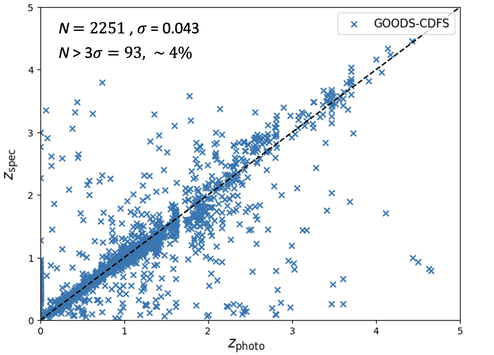
Figure 1: Comparison of spectroscopic and photometric redshifts using deep optical and NIR photometry from the GOODS CDF-S survey (Wuyts et al., 2008). Here the outlier fraction is defined as $|z_{\text{spec}}-z_{\text{photo}}|/(1+z_{\text{spec}})>3\sigma$ (see Section 4 for more details), which is about 4%. We expect many of these outliers to be DSFGs, and more accurate photometric redshifts can be obtained by incorporating FIR and submm photometry.

2 Photometric redshift fitting in FIR/submm bands

The process of star formation involves dust, which is subsequently heated by nearby stars to produce a thermal SED peaking at around $100\,\mu$m in the rest frame; consequently, DSFGs are bright at FIR/submm wavelengths as this emission becomes redshifted (Franceschini et al., 1991; Blain & Longair, 1993). Herschel-SPIRE (Griffin et al., 2010) operated in three FIR bands centered on 250, 350, and 500 $\mu\text{m}$. It conducted wide surveys of the sky, providing SED information for tens of thousands of DSFGs, including those that are faint in the optical and NIR. Here we use SPIRE photometry as an example to describe how to constrain photometric redshifts. However, we note that our method can be generalised to photometry at arbitrary FIR/submm wavelengths.

2.1 Mathematical background

Considering that the rest-frame FIR emission from DSFGs is dominated by optically-thin dust (as reviewed by Casey et al., 2014), we can model the emitted flux density in the rest-frame across a bandwidth $d\nu_{\textrm{em}}$ as a modified blackbody function:

$$S_{\nu_{\textrm{em}}}(T_{\textrm{em}},A_{\textrm{em}})d\nu_{\textrm{em}}=A_{\textrm{em}}\frac{\nu_{\textrm{em}}^{3+\beta}}{\text{exp}(h\nu_{\textrm{em}}/kT_{\textrm{em})}-1}d\nu_{\textrm{em}}.$$ (1)

Here $h$ and $k$ are the Planck and Boltzmann constants, respectively, and $\beta$ is the dust emissivity index that we fix to a value of 2.

We know that the observed frequency $\nu_{\textrm{obs}}$ and the observed dust temperature temperature $T_{\textrm{obs}}$ are related to the emitted frequency $\nu_{\textrm{em}}$ and the emitted dust temperature $T_{\textrm{em}}$ by

$$\nu_{\textrm{em}}=\nu_{\textrm{obs}}(1+z),$$ (2)

$$T_{\textrm{em}}=T_{\textrm{obs}}(1+z),$$ (3)

hence we can rewrite Eq. 1 in terms of observed-frame quantities as

$$S_{\nu_{\textrm{obs}}}(T_{\textrm{obs}},A_{\textrm{obs}})d\nu_{\textrm{obs}}=A_{\textrm{obs}}\frac{\nu_{\textrm{obs}}^{3+\beta}}{\text{exp}(h\nu_{\textrm{obs}}/kT_{\textrm{obs}})-1}d\nu_{\textrm{obs}},$$ (4)

where we have used

$$A_{\textrm{obs}}=A_{\textrm{em}}(1+z)^{4+\beta}.$$ (5)

Using this SED model, we can determine the optimal values of the two unknown observed-frame parameters, $A_{\textrm{obs}}$ and $T_{\textrm{obs}}$, by fitting the model to the three SPIRE flux density measurements at 250, 350 and $500\text{\,}\mu\mathrm{m}$. Here we fit for these parameters using a Markov chain Monte Carlo (MCMC).

It is worth mentioning that when converting to the emitted frame, $T_{\textrm{em}}$ and $1+z$ are entirely degenerate, since $\nu_{\textrm{obs}}/T_{\textrm{obs}}=\nu_{\textrm{em}}/T_{\textrm{em}}$. Therefore, obtaining a redshift estimate necessitates knowledge of $T_{\textrm{em}}$, and the uncertainty in the redshift estimation is primarily driven by the broad intrinsic temperature distribution (e.g., Wuyts et al., 2008). Nevertheless, we can improve the accuracy of the redshift estimate by incorporating information from the luminosity, as we now show.

In general, a luminosity $L$ can be related to a flux (the flux density integrated over a given wavelength range) by

$$L=4\pi D_{\textrm{L}}(z)^{2}F,$$ (6)

where $D_{\textrm{L}}$ is the luminosity distance. A common wavelength range comes from defining the ‘total’ infrared luminosity as the integral from 8 to $1000\text{\,}\mathrm{\SIUnitSymbolMicro m}$ in the rest frame, so that

$$L_{\textrm{IR}}=4\pi D_{\textrm{L}}(z)^{2}F_{\textrm{IR}}=4\pi D_{\textrm{L}}(z)^{2}\int_{1000}^{8}S_{\nu_{\textrm{em}}}d\nu_{\textrm{em}}.$$ (7)

Note that ‘8’ and ‘1000’ should be understood to mean the frequencies associated with these wavelengths in $\mu$m.

Next, we have a constraint equation given by the observed correlation between the temperature and the total infrared luminosity of galaxies. Following studies of this correlation in nearby and distant infrared-luminous galaxies (e.g. Chapin et al., 2009), we model this as a power law (although the functional form could be more general):

$$L_{\textrm{IR}}=f(T_{\textrm{em}})=\alpha T_{\textrm{em}}^{\gamma}.$$ (8)

Finally, since

$$F_{\textrm{IR}}=\frac{L_{\textrm{IR}}}{4\pi D_{\textrm{L}}(z)^{2}}=\int_{1000}^{8}S_{\nu_{\textrm{em}}}(T_{\textrm{em}},z)d\nu_{\textrm{em}}\ ,$$ (9)

we can substitute Eqs. 1, 5, and 8 to obtain

$$A_{\textrm{obs}}=\left(\frac{\alpha T_{\textrm{em}}^{\gamma}}{4\pi D_{\textrm{L}}(z)^{2}}\ \right)\Big{/}\\ \left(\int_{1000}^{8}\left(\frac{\nu_{\textrm{em}}}{1+z}\right)^{3+\beta}\left[\text{exp}\left(\frac{h\nu_{\textrm{em}}}{kT_{\textrm{em}}}\right)-1\right]^{-1}\frac{d\nu_{\textrm{em}}}{1+z}\right).$$ (10)

The goal now is to go from the space of observed amplitude ($A_{\textrm{obs}}$) and observed temperature ($T_{\textrm{obs}}$), to the space of redshift ($z$) and emitted temperature ($T_{\textrm{em}}$). We can do this using a Jacobian transformation:

$$p(z,T_{\textrm{em}})\,dz\,dT_{\textrm{em}}=$$

$$p[A_{\textrm{obs}}(z,T_{\textrm{em}}),T_{\textrm{obs}}(z,T_{\textrm{em}})]\cdot\textrm{det}\begin{vmatrix}\frac{\partial A_{\textrm{obs}}}{\partial z}&\frac{\partial A_{\textrm{obs}}}{\partial T_{\textrm{em}}}\\ \frac{\partial T_{\textrm{obs}}}{\partial z}&\frac{\partial T_{\textrm{obs}}}{\partial T_{\textrm{em}}}\end{vmatrix}dz\,dT_{\textrm{em}}.$$ (11)

This can then be marginalized over $T_{\textrm{em}}$ to produce a one-dimensional probability density function (PDF) for redshift, $p(z)$. Let us calculate each cell of this Jacobian explicitly using Eqs. 3 and 10. Firstly,

$$\frac{\partial A_{\textrm{obs}}(z,T_{\textrm{em}})}{\partial z}=\\ \frac{\partial}{\partial z}\left[\frac{1}{\int_{1000}^{8}S_{\nu_{\textrm{em}}}(T_{\textrm{em}},z)\,d\nu_{\textrm{em}}}\right]\frac{f(T_{\textrm{em}})}{4\pi D_{\textrm{L}}(z)^{2}}\\ +\frac{1}{\int_{1000}^{8}S_{\nu_{\textrm{em}}}(T_{\textrm{em}},z)\,d\nu_{\textrm{em}}}\frac{\partial}{\partial z}\left[\frac{f(T_{\textrm{em}})}{4\pi D_{\textrm{L}}(z)^{2}}\right]\\ =-\frac{\left(\int_{1000}^{8}\frac{\partial}{\partial z}S_{\nu_{\textrm{em}}}(T_{\textrm{em}},z)\,d\nu_{\textrm{em}}\right)}{\left(\int_{1000}^{8}S_{\nu_{\textrm{em}}}(T_{\textrm{em}},z)\,d\nu_{\textrm{em}}\right)^{2}}\frac{f(T_{\textrm{em}})}{4\pi D_{\textrm{L}}(z)^{2}}\\ +\frac{1}{\int_{1000}^{8}S_{\nu_{\textrm{em}}}(T_{\textrm{em}},z)\,d\nu_{\textrm{em}}}\left[\frac{-2f(T_{\textrm{em}})}{4\pi D_{\textrm{L}}(z)^{2}}\frac{\partial D_{\textrm{L}}(z)}{\partial z}\right],$$ (12)

where $\partial D_{\textrm{L}}(z)/\partial z$ can be performed numerically assuming Planck Collaboration (2018) cosmological parameters. The partial derivative is given by

$$\frac{\partial}{\partial z}[S_{\nu_{\textrm{em}}}(T_{\textrm{em}},z)d\nu_{\textrm{em}}]=\\ -(4+\beta)\left(\frac{1}{1+z}\right)^{5+\beta}\frac{\nu_{\textrm{em}}^{(3+\beta)}}{\text{exp}\left(\frac{h\nu_{\textrm{em}}}{kT_{\textrm{em}}}\right)-1}.$$ (13)

The next term in the Jacobian is

$$\frac{\partial A_{\textrm{obs}}(z,T_{\textrm{em}})}{\partial T_{\textrm{em}}}=\\ \frac{\partial}{\partial T_{\textrm{em}}}\left[\frac{1}{\int_{1000}^{8}S_{\nu_{\textrm{em}}}(T_{\textrm{em}},z)d\nu_{\textrm{em}}}\right]\frac{f(T_{\textrm{em}})}{4\pi D_{\textrm{L}}(z)^{2}}\\ +\frac{1}{\int_{1000}^{8}S_{\nu_{\textrm{em}}}(T_{\textrm{em}},z)d\nu_{\textrm{em}}}\frac{\partial}{\partial T_{\textrm{em}}}\left[\frac{f(T_{\textrm{em}})}{4\pi D_{\textrm{L}}(z)^{2}}\right]\\ =-\frac{\left(\int_{1000}^{8}\frac{\partial}{\partial T_{\textrm{e}}}S_{\nu_{\textrm{em}}}(T_{\textrm{em}},z)d\nu_{\textrm{em}}\right)}{\left(\int_{1000}^{8}S_{\nu_{\textrm{em}}}(T_{\textrm{em}},z)d\nu_{\textrm{em}}\right)^{2}}\frac{f(T_{\textrm{em}})}{4\pi D_{\textrm{L}}(z)^{2}}\\ +\frac{1}{\int_{1000}^{8}S_{\nu_{\textrm{em}}}(T_{\textrm{em}},z)d\nu_{\textrm{em}}}\left[\frac{1}{4\pi D_{\textrm{L}}(z)^{2}}\frac{\partial f(T_{\textrm{em}})}{\partial T_{\textrm{em}}}\right],$$ (14)

and the remaining partial derivatives are

$$\frac{\partial}{\partial T_{\textrm{em}}}S_{\nu_{\textrm{em}}}(T_{\textrm{em}},z)=\\ \left(\frac{1}{1+z}\right)^{4+\beta}\frac{\nu_{\textrm{em}}^{(3+\beta)}}{\left[\text{exp}\left(\frac{h\nu_{\textrm{em}}}{kT_{\textrm{em}}}\right)-1\right]^{2}}\left(\frac{h\nu_{\textrm{em}}}{kT_{\textrm{em}}^{2}}\right)\text{exp}\left(\frac{h\nu_{\textrm{em}}}{kT_{\textrm{em}}}\right),$$ (15)

$$\frac{\partial f(T_{\textrm{em}})}{\partial T_{\textrm{em}}}=\alpha\gamma T_{\textrm{em}}^{\gamma-1}.$$ (16)

The last two terms in the Jacobian are derivatives with respect to the observed temperature, and are given by

$$\frac{\partial T_{\textrm{obs}}}{\partial z}=-\frac{T_{\textrm{em}}}{(1+z)^{2}}$$ (17)

and

$$\frac{\partial T_{\textrm{obs}}}{\partial T_{\textrm{em}}}=\frac{1}{1+z}.$$ (18)

By explicitly computing the Jacobian, multiplying by the two-dimensional function $p[A_{\textrm{obs}}(z,T_{\textrm{em}}),T_{\textrm{obs}}(\textrm{z},T_{\textrm{em}})]$, and marginalizing over the range of $T_{\textrm{em}}$, we obtain

$$p(z)=\int p[A_{\textrm{obs}}(z,T_{\textrm{em}}),T_{\textrm{obs}}(z,T_{\textrm{em}})\times\\ \left[\frac{\partial A_{\textrm{obs}}}{\partial z}\frac{\partial T_{\textrm{obs}}}{\partial T_{\textrm{em}}}-\frac{\partial A_{\textrm{obs}}}{\partial T_{\textrm{em}}}\frac{\partial T_{\textrm{obs}}}{\partial z}\right]dT_{\textrm{em}}.$$ (19)

The luminosity-temperature relation is of course not exact, therefore it is important to also marginalize over a width representing the intrinsic variance of galaxy infrared luminosities for a given temperature. To incorporate the scatter in the relation, during the MCMC process we also draw a Gaussian random variable with a mean centered at $\alpha$ and a standard deviation of $0.22\alpha$ (as explained in the next subsection and shown in Fig. 2, also see subsection 3.2 of Chapin et al. 2009). We then recalculate the Jacobian for each new $\alpha$, thus marginalizing over the intrinsic dispersion in the luminosity-temperature relation, which effectively increases the width of the redshift probability distribution. It is worth pointing out that the slope $\gamma$ could also be uncertain and potentially correlated with $\alpha$, but we are ignoring this for now.

A key difference between this work and Aretxaga et al. (2003) is that we do not include any priors based on the expected redshift distribution for a given survey catalog. This is achieved in Aretxaga et al. (2003) by incorporating a range of SED templates and an empirical model for the evolution of the luminosity function in the context of the expanding Universe. Simulated galaxies are randomly drawn from this model with the appropriate survey parameters (such as flux limits at particular wavelengths) for comparison with observations of real galaxies selected in the same way. The posterior redshift PDF of a real galaxy is then derived from the redshifts of simulated galaxies with similar observed flux densities and colors. Redshifts with few (or no) galaxies in the simulated catalogue will thus be heavily down-weighted. Such priors (if well-characterized) have the potential to yield estimates with narrower distributions (particularly for submillimeter surveys considered in isolation). Instead, our method simply assigns a greater weight to redshift estimates if the implied rest-frame luminosity and temperature are plausible. While this approach uses less information (and may therefore yield broader distributions), we believe it provides sufficient constraining power to reject catastrophic failures from otherwise optical and NIR-based photometric redshifts, as we will show. In future, as we obtain more information on the evolving luminosity function, we could add redshift priors.

To summarize, we use the three SPIRE photometric points to estimate two observed parameters, namely the peak frequency and amplitude, and then relate them to intrinsic quantities $T_{\textrm{em}}$ and $z$ using the luminosity-temperature relation, and include an additional marginalization over the amplitude of this relation.

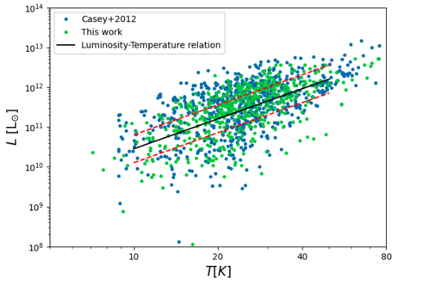
Figure 2: FIR luminosity versus dust temperature. The blue points are taken directly from Casey et al. (2012), while the green points are our calculated luminosities, obtained by fitting the same SPIRE flux densities to Eq. 1 and integrating. The best-fit power-law provides our luminosity-temperature relation, shown in black. The dashed red lines represent the estimated intrinsic scatter (after removing the scatter due to statistical errors) and are given by ${\pm}0.22\alpha$.

2.2 The galaxy luminosity-temperature relation

To find the luminosity-temperature constraint parameters $\alpha$ and $\gamma$, we need to know the spectroscopic redshifts and emitted temperatures of a sample of galaxies. This correlation has been investigated by Chapin et al. (2009) and Casey et al. (2012); the former used a sample of IRAS-selected low-$z$ galaxies, and the latter used a sample of Herschel-selected galaxies out to $z\,{=}\,2$. Here we primarily make use of the sample from Casey et al. (2012); Fig. 2 shows the resulting luminosity-temperature correlation of their sample (using both the luminosity and temperature values provided in the paper and our own best-fit values using Eqs. 3 and 4). We find a best-fit amplitude of $\alpha\,{=}\,10^{7.95}$ and a best-fit slope of $\gamma\,{=}\,2.50$, and we confirm that our luminosity-temperature relation agrees with the results from the low-$z$ sample of Chapin et al. (2009) by comparing with their Figure 4 (after implementing the necessary transformations, such as converting far-IR color to temperature).

In addition, we use the sample of SPIRE-selected galaxies from Casey et al. (2012) to estimate the intrinsic scatter in the relation by symmetrically adjusting $\alpha$ about its best-fit value until $68\%$ of the galaxies fall within the lower and upper bounds, finding a range of $\pm 0.35$ dex. This value is the uncertainty due to both intrinsic scatter and statistical noise in the SPIRE data, and for our photo-z marginalizations we only want to take into account the intrinsic scatter. The median uncertainty in the $L_{\textrm{IR}}$ measurements of the sample was found to be 0.27 dex, thus the intrinsic scatter is $\sqrt{0.35^{2}\,{-}\,0.27^{2}}\,{=}\,0.22$ dex.

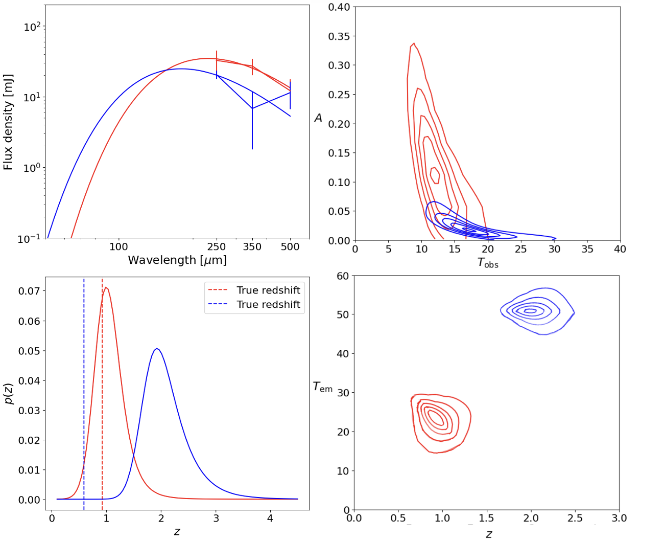
Figure 3: Comparison between two galaxies, one with three submm flux density measurements that correctly identifies the peak of the modified blackbody function and leads to a reliable redshift estimate (red colour), while the three fluxes of the galaxy in blue does not identify the peak of the function, which leads to an inaccurate estimate of the redshift. The contour plot of $A_{\textrm{obs}}$ and $T_{\textrm{obs}}$ (top right) are transformed using Eq. 2.1 to obtain the corresponding contour plot for $T_{\textrm{em}}$ and $z$ (bottom right). The resulting redshift PDF are shown with solid red and blue lines while the actual redshift values are shown by dashed lines.

It is important to point out that biases in the sample used to calibrate the luminosity-temperature relation could result in inaccurate photo-z estimation. For instance, the redshifts in the Casey et al. (2012) sample are limited to values below 2, with the majority concentrated between 0.6 and 0.9. Consequently, when using this method to predict redshifts based on three SPIRE flux densities, predictions tend to cluster within this range. This observation is reinforced using simulated data, revealing a decrease in prediction reliability for galaxies at higher redshifts (in this case $z>2$). This arises from the fact that the luminosity-temperature fit parameters are derived primarily from galaxies at lower redshifts. The method works well when applied to galaxies with similar redshifts as those used to establish the correlation parameters, and the range can be extended with future data sets. What we describe here is only an example.

2.3 Submm/mm SED fitting

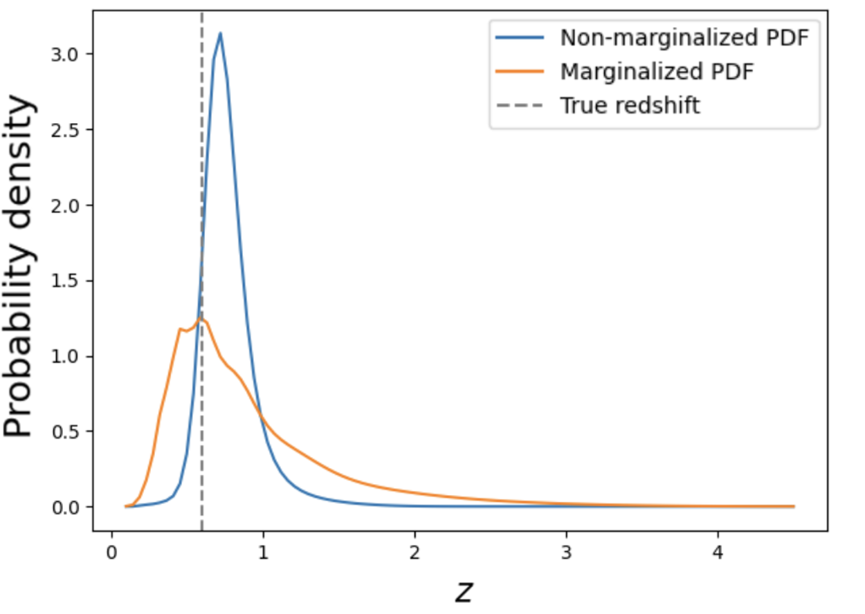
Figure 4: An example showing the effect of marginalizing over $\alpha$ (see Eq. 8). The blue PDF is generated assuming that the luminosity-temperature relation is exact, while the orange PDF is computed by marginalizing over the amplitude of the luminosity-temperature relation.

We fit the observed quantities with a standard MCMC method with no priors on the parameters using Python’s lmfit, Newville et al. (2021), and minimize using the ‘emcee’ method. The likelihood function is therefore simply given by $\exp(-\chi^{2}/2)$. After transforming from the 2D parameter space $(A_{\textrm{obs}},T_{\textrm{obs}})$ to $(T_{\textrm{em}},z)$, we obtain the PDF $p(z)$ by marginalizing over $T_{\textrm{em}}$.

Given the limited amount of information provided by only three submm data points, we can make accurate inferences about the shape of the SED only if these points provide meaningful information about the curvature of the SED. However, when all three flux density points are situated deep into the Rayleigh-Jeans or Wien side of the modified blackbody peak, or if blending with nearby galaxies contaminates the photometry, it is difficult to determine the peak position and amplitude. Figures 3 provide an illustration of two scenarios: one with three flux densities containing meaningful curvature information, which yields a good constraint; and the other where the flux densities have been contaminated by source blending. In cases where the modified blackbody model provides a poor fit (which we take to be $\chi^{2}\,{>}\,3$ ), we disregard the FIR redshift PDF and only use the results from optical photometry. As discussed above, we also include an additional marginalization over $\alpha$ due to the intrinsic scatter in the luminosity-temperature relation, which broadens the probability distribution; and example of this is shown in Fig. 4.

3 Combining FIR/submm and optical/NIR photometric redshifts

Although usually much more accurate than with submm data alone, photometric redshift estimation using NIR and optical photometry is considerably more complicated because of the variety of SEDs, requiring more parameters. The two standard approaches are the empirical method, which uses a training set to fit for the parameters of a simple function, and the SED template-fitting technique, which uses a library of possible template SEDs (for example from Bruzual & Charlot, 2003).

To achieve our objective of combining optical photometric redshifts with submm photometric redshifts, we employ a code that uses the SED template-fitting approach. Specifically, we use the Easy Accurate zphoto from Yale (EAzY; Brammer et al., 2010) code, which computes linear combinations of SED templates in the optical-to-NIR over the redshift range of $0$–$4$. Importantly, the output of EAzY is a redshift PDF, which we can multiply by our FIR/submm redshift PDFs to obtain a final redshift estimate as the two distributions are completely independent.

We ran EAzY using the default parameter file, which is designed to provide an optimized template set, template error function, and priors for most applications. While the majority of galaxy redshift estimates produced by EAzY will exhibit a single, well-defined peak, certain cases can yield multiple peaks due to degeneracies in the model parameters. This is can be particularly pronounced when dealing with specific subsets of galaxies, such as DSFGs or active galactic nuclei (AGN). Notably, galaxies with relatively featureless SEDs can equally match observations at both $z\sim 1$ and $z\sim 3$ (e.g., Roseboom et al., 2011), and an illustrative example of this is presented in Fig. 5.

Finally, Fig. 6 shows an example of combining (i.e. multiplying) the results from both FIR/submm SED fitting and optical/NIR SED fitting. This particular example is a galaxy bright in the SPIRE wavelengths and faint in the optical, and we see that the photometric redshift estimate is improved by including longer-wavelength information.

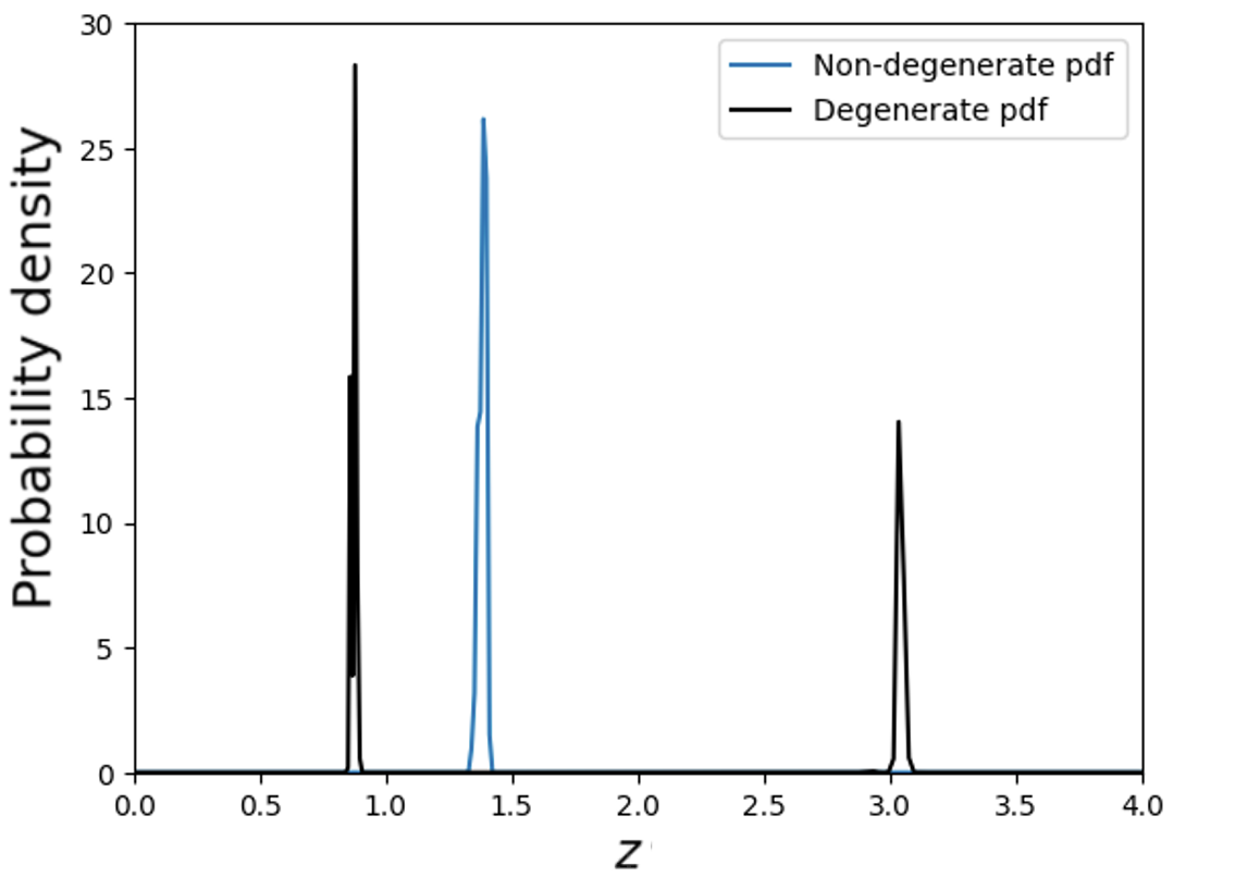
Figure 5: Example redshift PDFs generated using EAzY. The black PDF illustrates a case of a galaxy with degenerate redshift values, whereas the blue PDF shows a galaxy with a distinct, non-degenerate (single) peak. We expect many DSFGs to fall in the former case, and we can break the degeneracy with information from FIR/submm wavelengths.

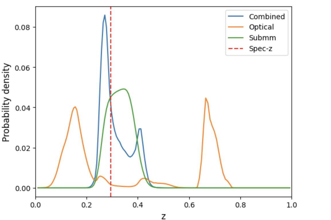
Figure 6: Example redshift PDFs from EAzY, FIR photometry and the their combination (i.e. the product of the two probabilities), compared to the spectroscopic redshift.

4 Applications to real galaxy catalogues

4.1 Test catalogues

To test our proposed method for combining optical/NIR photometry with FIR/submm photometry, we use the ‘super-deblended’ galaxy sample in the COSMOS field (Jin et al., 2018). This catalogue uses optically-selected galaxies as priors to fit PSFs to Herschel-SPIRE data, thus providing the necessary optical-through-FIR photometry needed to test our proposed photometric-estimation method. The final deblendeded catalog includes 11,220 galaxies over the 100–1200 $\mu$m range, extending to redshifts above 4. Out of these galaxies, we selected about 5% (600) of the brighter galaxies ($K<22.5$) that have reliable optical/NIR photometry and spectroscopic redshift from COSMOS 2015 (Laigle et al., 2016).

This ‘super-deblended’ catalog is purely optically-selected. We also test our method using a purely FIR-selected sample of galaxies with redshifts between 0 and 1 from the Herschel Astrophysical Terahertz Large Area Survey (H-ATLAS), extensively detailed in Valiante et al. (2016) and Bourne et al. (2016). This survey spans three fields covering a total area of 161.6 deg² along the celestial equator with each field spanning approximately 54 deg², and contains overlapping optical/NIR imaging. This catalog, which is a subset of the gamma field of H-ATLAS, contains 120,230 sources selected at 250, 350, and $500\text{\,}\mu\mathrm{m}$, along with photometry for their optical and NIR counterparts. After filtering for all the galaxies with reliable redshift, as well as optical and submm photometric bands, we selected a random sample of 250 of the brighter galaxies for this analysis.

4.2 Catastrophic outlier metric

We define the catastrophic outlier fraction, $\eta$, to be the fraction of sources with an unexpectedly large difference between the photometric and spectroscopic redshift. This is explicitly given by

$$\delta z>3\sigma,$$ (20)

where

$$\delta z=\frac{\left|z_{\text{photo}}-z_{\text{spec}}\right|}{1+z_{\text{spec}}}$$ (21)

and

$$\sigma=1.48\times\text{median}\left(\left|\frac{\Delta z-\text{median}(\Delta z)}{1+z_{\text{spec}}}\right|\right),$$ (22)

with $\Delta z=z_{\text{photo}}-z_{\text{spec}}.$ We have chosen this definition of $\sigma$ as it is less sensitive to outliers than the usual definition of the standard deviation (Brammer et al., 2010).

4.3 Results

We want to demonstrate that our method improves photo-$z$ estimates for existing samples of galaxies. However, a challenge is that we can only test how well the estimates improve photo-$z$s if we have spec-$z$s for the sources. Good spectroscopic redshifts are still scarce for submm-selected galaxies, while optically-selected catalogues with good spectroscopy often have such good photo-$z$s that the submm data hardly help. We therefore start with an optically-selected sample, and artificially degrade it to represent a catalog with only moderately-constraining optical/NIR photometry.

For this test, we use a subset of six Euclid-like photometric bands (B, R, Ks, J, H, and Y) from the ‘super-deblended’ catalog, and artificially increase the noise by a factor of 3 in order to simulate the type of data expected from future wide field surveys. The results are shown in Fig. 7; we see that while the fraction of catastrophic outliers is already low for these optically-bright galaxies, using submm photometry is still able to reduce the fraction further.

We also tested this result by using the original ‘super-deblended’ catalogue (without removing bands or changing the noise). However, including submm bands did not provide a significant improvement, since the photometric redshifts of these optically-bright galaxies were already very closely aligned with the spectroscopic redshifts.

Figure 7: Spec-zs versus photo-zs for a sample of 630 ‘super-deblended’ galaxies in the COSMOS field from Jin et al. (2018), artificially degraded by restricting the optical/NIR photometry to six bands and increasing the noise by a factor of 3. Photometric redshifts using optical and NIR data with EAzY alone are shown in blue, while photometric redshifts after combining with submm data are shown in orange. Here the fraction of outliers for the blue data is $9.1\%$, while for the orange data is $6.3\%$.

We next turn to galaxies selected by SPIRE. For this test we used the U, G, R, I, Ks, J, H, Y, and Z bands. The result of applying our algorithm to the H-ATLAS catalog is shown in Fig. 8. Without adjusting any of the optical/NIR photometry, we find that the number of catastrophic outliers reduces from 23 (9.2%) to 8 (3.2%), showing a significant improvement in photometric redshift estimation.

Figure 8: Spec-z versus photo-z for a sample of 250 bright submm galaxies taken from the H-ATLAS catalog (Valiante et al., 2016; Bourne et al., 2016). The inclusion of submm bands provides a significant reduction in catastrophic outliers, with three times fewer outliers compared to using only optical and NIR bands.

4.4 Future Improvements

While in this paper we used the specific example of Herschel-SPIRE photometry, our approach is general, and adding more submm photometric points (e.g., $850\,\mu$m data from SCUBA-2) would further improve our method. Additionally, as we learn more about the relevant galaxy populations, from Euclid and Rubin surveys for example, we can continually update the $L$–$T$ relation, thus improving the submm photo-$z$ estimates.

Finally, we can also include a volume prior to better capture the galaxy population distribution, similar to the work done by Aretxaga et al. (2003). Incorporating this prior here would not have made a significant difference because our test catalogue of galaxies do not span a very large redshift range. However, with future data sets spanning a wider redshift range, the use of a volume prior will be much more important.

5 Conclusions

The primary objective of this paper is to enhance photometric redshift estimates, specifically targeting the dustiest and most actively star-forming galaxies where conventional optical and NIR fits sometimes fall short. In a broader context, our aim aligns with the overarching goal of obtaining accurate redshift estimates for all galaxies in large surveys. Achieving this objective necessitates significant improvement in photo-z accuracy, particularly for sources where optical and NIR fits are unreliable.

The largest photo-z galaxy samples in the near future are going to come from the Euclid and Rubin surveys. There is a strong emphasis on the use of galaxies for cosmological studies involving gravitational lensing and clustering, and hence galaxies with challenging photometric redshifts will tend to be excluded. However, for studies of galaxy evolution, we certainly do not want to throw away the DSFGs, AGN and high-redshift galaxies. This is where the approach described in this paper will be most useful; by including high-quality wide-field submm data from future facilities like CCAT, we can build more complete redshift catalogues of galaxies applicable for a wide range of studies in galaxy evolution, thus improving the long-term impact of these surveys.

References

- Aretxaga et al. (2003) Aretxaga, I., Hughes, D. H., Chapin, E. L., et al. 2003, MNRAS, 342, 759, doi: 10.1046/j.1365-8711.2003.06560.x
- Baum (1957) Baum, W. A. 1957, AJ, 62, 6, doi: 10.1086/107433
- Blain & Longair (1993) Blain, A. W., & Longair, M. S. 1993, Monthly Notices of the Royal Astronomical Society, 264, 509, doi: 10.1093/mnras/264.2.509
- Blain et al. (2002) Blain, A. W., Smail, I., Ivison, R. J., Kneib, J. P., & Frayer, D. T. 2002, Phys. Rep., 369, 111, doi: 10.1016/S0370-1573(02)00134-5
- Boquien et al. (2019) Boquien, M., Burgarella, D., Roehlly, Y., et al. 2019, A&A, 622, A103, doi: 10.1051/0004-6361/201834156
- Bourne et al. (2016) Bourne, N., Dunne, L., Maddox, S. J., et al. 2016, MNRAS, 462, 1714, doi: 10.1093/mnras/stw1654
- Brammer et al. (2010) Brammer, G. B., van Dokkum, P. G., & Coppi, P. 2010, EAZY: A Fast, Public Photometric Redshift Code, Astrophysics Source Code Library, record ascl:1010.052
- Bruzual & Charlot (2003) Bruzual, G., & Charlot, S. 2003, MNRAS, 344, 1000, doi: 10.1046/j.1365-8711.2003.06897.x
- Carilli & Yun (1999) Carilli, C. L., & Yun, M. S. 1999, The Astrophysical Journal, 513, L13–L16, doi: 10.1086/311909
- Casey et al. (2012) Casey, C. M., Berta, S., Béthermin, M., et al. 2012, ApJ, 761, 140, doi: 10.1088/0004-637X/761/2/140
- Casey et al. (2014) Casey, C. M., Narayanan, D., & Cooray, A. 2014, Phys. Rep., 541, 45, doi: 10.1016/j.physrep.2014.02.009
- CCAT-Prime Collaboration et al. (2023) CCAT-Prime Collaboration, Aravena, M., Austermann, J. E., et al. 2023, ApJS, 264, 7, doi: 10.3847/1538-4365/ac9838
- Chakrabarti et al. (2013) Chakrabarti, S., Magnelli, B., McKee, C. F., et al. 2013, ApJ, 773, 113, doi: 10.1088/0004-637X/773/2/113
- Chapin et al. (2009) Chapin, E. L., Hughes, D. H., & Aretxaga, I. 2009, Monthly Notices of the Royal Astronomical Society, 393, 653, doi: 10.1111/j.1365-2966.2008.14242.x
- Euclid Collaboration: Mellier et al. (2024) Euclid Collaboration: Mellier, Y., Abdurro’uf, Acevedo Barroso, J. A., et al. 2024, arXiv e-prints, arXiv:2405.13491, doi: 10.48550/arXiv.2405.13491
- Franceschini et al. (1991) Franceschini, A., Toffolatti, L., Mazzei, P., Danese, L., & de Zotti, G. 1991, A&AS, 89, 285
- Griffin et al. (2010) Griffin, M. J., Abergel, A., Abreu, A., et al. 2010, A&A, 518, L3, doi: 10.1051/0004-6361/201014519
- Ilbert et al. (2008) Ilbert, O., Capak, P., Salvato, M., & Aussel, H. 2008, The Astrophysical Journal, 690, 1236, doi: 10.1088/0004-637x/690/2/1236
- Ivezić et al. (2019) Ivezić, Ž., Kahn, S. M., Tyson, J. A., et al. 2019, ApJ, 873, 111, doi: 10.3847/1538-4357/ab042c
- Jin et al. (2018) Jin, S., Daddi, E., Liu, D., et al. 2018, The Astrophysical Journal, 864, 56
- Koprowski et al. (2017) Koprowski, M. P., Dunlop, J. S., Michałowski, M. J., et al. 2017, MNRAS, 471, 4155, doi: 10.1093/mnras/stx1843
- Laigle et al. (2016) Laigle, C., McCracken, H. J., Ilbert, O., et al. 2016, ApJS, 224, 24, doi: 10.3847/0067-0049/224/2/24
- Lim et al. (2020) Lim, C.-F., Chen, C.-C., Smail, I., et al. 2020, ApJ, 895, 104, doi: 10.3847/1538-4357/ab8eaf
- Nayyeri et al. (2017) Nayyeri, H., Hemmati, S., Mobasher, B., et al. 2017, The Astrophysical Journal Supplement Series, 228, 7, doi: 10.3847/1538-4365/228/1/7
- Newman & Gruen (2022) Newman, J. A., & Gruen, D. 2022, ARA&A, 60, 363, doi: 10.1146/annurev-astro-032122-014611
- Newville et al. (2021) Newville, M., Otten, R., Nelson, A., et al. 2021, Lmfit/lmfit-py: 1.0.3, 1.0.3, Zenodo, doi: 10.5281/zenodo.5570790
- Planck Collaboration (2018) Planck Collaboration. 2018, arXiv e-prints. https://arxiv.org/abs/1807.06209
- Roseboom et al. (2011) Roseboom, I. G., Ivison, R. J., Greve, T. R., et al. 2011, Monthly Notices of the Royal Astronomical Society, 419, 2758
- Salvato et al. (2019) Salvato, M., Ilbert, O., & Hoyle, B. 2019, Nature Astronomy, 3, 212, doi: 10.1038/s41550-018-0478-0
- Valiante et al. (2016) Valiante, E., Smith, M. W. L., Eales, S., et al. 2016, MNRAS, 462, 3146, doi: 10.1093/mnras/stw1806
- van Dokkum et al. (2011) van Dokkum, P. G., Brammer, G., Fumagalli, M., et al. 2011, ApJ, 743, L15, doi: 10.1088/2041-8205/743/1/L15
- Wuyts et al. (2008) Wuyts, S., Labbé, I., Schreiber, N. M. F., et al. 2008, The Astrophysical Journal, 689, 653, doi: 10.1086/592773
- Yee (1998) Yee, H. 1998, arXiv: Astrophysics